Simulation and Control of Submarines - Lunds...

Department of Automatic Control

Simulation and Control of Submarines

Erik Lind

Magnus Meijer

MSc Thesis ISRN LUTFD2/TFRT--5954--SE ISSN 0280-5316

Department of Automatic Control Lund University Box 118 SE-221 00 LUND Sweden

© 2014 by Erik Lind & Magnus Meijer. All rights reserved. Printed in Sweden by Media-Tryck Lund 2014

Abstract

When designing control systems for real applications, it is important to first do test-ing in a simulated environment, to ensure adequate performance. This is especiallyimportant when designing control systems for applications that have high operationcosts, e.g., submarines, since late errors in the development can be extremely costly.

Saab develops steering systems for submarines. Prior to this thesis, testing forthose have been performed in an open-loop environment, where only static test casescould be examined. Saab therefore identified the need to implement a dynamic testsimulator, which could react to the different signals from the steering system, i.e.,act as a real submarine.

In this thesis, such a simulator was developed. It consists of two parts, a physicalmodel of a submarine, and a control system for motion control. As for the physicalsubmarine model, it can be approximated from mechanical data of a submarine thatthe user provide, such as dimensions and weight. The second options is for the userto explicitly supply the simulator with hydrodynamic coefficients.

The control system was derived to control a model of a demo submarine. Saabis also involved in submarine navigation systems and saw the need to, in the future,also have the possibility to test those products. A navigation system assumes anautopilot exists, hence, an autopilot control system was developed.

In the end, the control system consisted of a two-level cascade controller ofmixed LQG- and PID-control, along with a Kalman estimator for estimating un-known states.

The results were overall satisfactory. The performance of the control system iswell within usual customer specifications and the main problems in this thesis layin getting a proper model.

3

Sammandrag

När styrsystem utvecklas för dyra applicationer, är det ofta viktigt att först uförasimulerade modelltester för att tidigt hitta fel och testa prestanda. På en ubåt ärdetta extra viktigt, eftersom fel som uppstår sent i utvecklingen kan bli väldigt kost-samma.

Saab utvecklar styrsystem till ubåtar. Innan detta examensarbete utfördes allatester på dessa produkter i en statisk miljö, där en användare kunde skicka ininsignaler till styrsystemet och studera utsignalerna från detta. Men användaren varsjälv tvungen att ändra på alla insignalerna för att studera ett annat fall. Saab sågdärför behovet av en dynamisk simulator som kunde reagera på utsignalerna frånstyrsystemet, det vill säga, replikera en riktig ubåt.

I det här examensarbetet utvecklades en sådan simulator. Den består av två delar,en fysikalisk modell av en ubåt och en autopilot för att styra dess rörelser. För denfysikaliska modellen finns möjligheten att få en approximerad modell av en ubåtutifrån fysiska mått. Den andra möjligheten är att användaren förser simulatorn medalla hydrodynamiska koefficienter.

Autopiloten utvecklades att styra en demoubåt. Saab är också involverade i navi-gationssystem till ubåtar, och såg därför behovet av att i framtiden också kunna testasådana produkter. Ett navigationssystem antar att det finns något som styr ubåtensrörelser, därför utvecklades också en autopilot.

Till slut bestod autopiloten av en kaskadregleringsdesign, där både LQG- ochPID-reglering används, tillsammans med en Kalmanestimator för att skatta deokända tillstånden.

Resultaten var överlag goda. Prestandan på styrsystemet låg väl inom normalakundkrav, och de största problemen låg i att få fram en god modell.

4

Acknowledgements

The authors would like to offer our deepest gratitude to Saab Group for the oppor-tunity to perform this thesis, and to get a valuable insight in engineering industry.Naturally, we would also like to thank Hans Bohlin at Saab who worked out the ideabehind this master thesis, and has also been our supervisor at Saab. He has been agreat mentor and has provided valuable help and assistance throughout this thesis.

Bo Carlsson assisted us with the implementation in C, this thesis would not havereached its final form without him.

We would also like to thank Mats Nordin and Lennart Bossér at FOI for the in-vitation to Stockholm. The meeting was very rewarding. Saab Underwater Systemsalso provided us with valuable tips and guidance, for which we are grateful for.

Finally, we would like to thank all the other nice people at Saab Support andServices for a pleasant time at Saab.

Erik Lind & Magnus Meijer27/6 2014 Malmslätt, Linköping

5

Contents

List of Figures 9List of Tables 111. Introduction 15

1.1 Submarines . . . . . . . . . . . . . . . . . . . . . . . . . . . . 151.2 Background . . . . . . . . . . . . . . . . . . . . . . . . . . . . 201.3 Thesis concepts . . . . . . . . . . . . . . . . . . . . . . . . . . 211.4 Scope of Master thesis . . . . . . . . . . . . . . . . . . . . . . . 211.5 Individual contribution . . . . . . . . . . . . . . . . . . . . . . 241.6 Thesis Outline . . . . . . . . . . . . . . . . . . . . . . . . . . . 24

2. Method 262.1 Coordinate System notation . . . . . . . . . . . . . . . . . . . . 262.2 Simulator development . . . . . . . . . . . . . . . . . . . . . . 262.3 Schedulers . . . . . . . . . . . . . . . . . . . . . . . . . . . . . 28

3. Theory 293.1 Hydrodynamics . . . . . . . . . . . . . . . . . . . . . . . . . . 293.2 6 degrees of freedom dynamics . . . . . . . . . . . . . . . . . . 353.3 Control designs . . . . . . . . . . . . . . . . . . . . . . . . . . 36

4. Development 394.1 Modelling of a submarine . . . . . . . . . . . . . . . . . . . . . 394.2 Generic submarine model . . . . . . . . . . . . . . . . . . . . . 464.3 Submarine demo model . . . . . . . . . . . . . . . . . . . . . . 504.4 Control design . . . . . . . . . . . . . . . . . . . . . . . . . . . 51

5. Results 655.1 Time constants and saturations . . . . . . . . . . . . . . . . . . 655.2 Final controller . . . . . . . . . . . . . . . . . . . . . . . . . . . 655.3 Simulation plots . . . . . . . . . . . . . . . . . . . . . . . . . . 67

6. Discussion 786.1 Hydrodynamic Coefficients discussion . . . . . . . . . . . . . . 786.2 Linearised state space model . . . . . . . . . . . . . . . . . . . 80

7

Contents

6.3 Controller issues . . . . . . . . . . . . . . . . . . . . . . . . . . 806.4 Future Work . . . . . . . . . . . . . . . . . . . . . . . . . . . . 82

Bibliography 85A. Appendix 87

A.1 Kt and Kq interpolation polynomials . . . . . . . . . . . . . . . 87

8

List of Figures

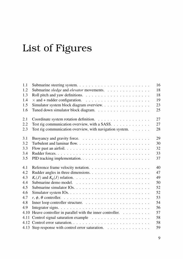
1.1 Submarine steering system. . . . . . . . . . . . . . . . . . . . . . . . 161.2 Submarine sledge and elevator movements. . . . . . . . . . . . . . . 181.3 Roll pitch and yaw definitions. . . . . . . . . . . . . . . . . . . . . . 181.4 × and + rudder configuration. . . . . . . . . . . . . . . . . . . . . . 191.5 Simulator system block diagram overview. . . . . . . . . . . . . . . . 231.6 Tuned down simulator block diagram. . . . . . . . . . . . . . . . . . 25

2.1 Coordinate system rotation definition. . . . . . . . . . . . . . . . . . 272.2 Test rig communication overview, with a SASS. . . . . . . . . . . . . 272.3 Test rig communication overview, with navigation system. . . . . . . 28

3.1 Buoyancy and gravity force. . . . . . . . . . . . . . . . . . . . . . . 293.2 Turbulent and laminar flow. . . . . . . . . . . . . . . . . . . . . . . . 303.3 Flow past an airfoil. . . . . . . . . . . . . . . . . . . . . . . . . . . . 323.4 Rudder forces. . . . . . . . . . . . . . . . . . . . . . . . . . . . . . . 333.5 PID tracking implementation. . . . . . . . . . . . . . . . . . . . . . . 37

4.1 Reference frame velocity notation. . . . . . . . . . . . . . . . . . . . 404.2 Rudder angles in three dimensions. . . . . . . . . . . . . . . . . . . . 474.3 Kt(J) and Kq(J) relation. . . . . . . . . . . . . . . . . . . . . . . . . 494.4 Submarine demo model. . . . . . . . . . . . . . . . . . . . . . . . . 504.5 Submarine simulator IOs. . . . . . . . . . . . . . . . . . . . . . . . . 524.6 Simulator system IOs. . . . . . . . . . . . . . . . . . . . . . . . . . . 524.7 r, φ , θ controller. . . . . . . . . . . . . . . . . . . . . . . . . . . . . 534.8 Inner loop controller structure. . . . . . . . . . . . . . . . . . . . . . 544.9 Integrator signs. . . . . . . . . . . . . . . . . . . . . . . . . . . . . . 564.10 Heave controller in parallel with the inner controller. . . . . . . . . . 574.11 Control signal saturation example . . . . . . . . . . . . . . . . . . . 584.12 Control error saturation. . . . . . . . . . . . . . . . . . . . . . . . . . 584.13 Step response with control error saturation. . . . . . . . . . . . . . . 59

9

List of Figures

4.14 Velocity regions, the shaded part is the hysteresis. . . . . . . . . . . . 594.15 Inner and outer loop control. . . . . . . . . . . . . . . . . . . . . . . 604.16 Integrator controller bandwidth. . . . . . . . . . . . . . . . . . . . . 614.17 Outer loop heading controller structure. . . . . . . . . . . . . . . . . 614.18 Outer loop depth control structure. . . . . . . . . . . . . . . . . . . . 624.19 Outer loop controller structure. . . . . . . . . . . . . . . . . . . . . . 64

5.1 Test case one, Heading. . . . . . . . . . . . . . . . . . . . . . . . . . 715.2 Test case one, Depth. . . . . . . . . . . . . . . . . . . . . . . . . . . 715.3 Test case one, Pitch. . . . . . . . . . . . . . . . . . . . . . . . . . . . 725.4 Test case one, Control Efforts. . . . . . . . . . . . . . . . . . . . . . 725.5 Test case two, Velocity. . . . . . . . . . . . . . . . . . . . . . . . . . 735.6 Test case two, Depth. . . . . . . . . . . . . . . . . . . . . . . . . . . 735.7 Test case two, Pitch. . . . . . . . . . . . . . . . . . . . . . . . . . . . 745.8 Test case two, Control Efforts. . . . . . . . . . . . . . . . . . . . . . 745.9 Test case three, Velocity. . . . . . . . . . . . . . . . . . . . . . . . . 755.10 Test case three, Heading. . . . . . . . . . . . . . . . . . . . . . . . . 755.11 Test case three, Position in the xy-plane. . . . . . . . . . . . . . . . . 765.12 Test case three, Control Efforts. . . . . . . . . . . . . . . . . . . . . . 765.13 Test case three, roll. . . . . . . . . . . . . . . . . . . . . . . . . . . . 775.14 RPS of the rotor vs. velocity. . . . . . . . . . . . . . . . . . . . . . . 77

6.1 Linear model in the high velocity region. . . . . . . . . . . . . . . . . 816.2 Rudder and submarine attitude animation. . . . . . . . . . . . . . . . 84

10

List of Tables

0.1 List of variables . . . . . . . . . . . . . . . . . . . . . . . . . . . . . 120.2 List of subscripts . . . . . . . . . . . . . . . . . . . . . . . . . . . . 140.3 List of coordinate systems . . . . . . . . . . . . . . . . . . . . . . . 140.4 List of abbreviations . . . . . . . . . . . . . . . . . . . . . . . . . . 14

3.1 Vector notation for six degrees of freedom . . . . . . . . . . . . . . . 36

4.1 Main data of the demo submarine. . . . . . . . . . . . . . . . . . . . 514.2 Controller features in the regions. . . . . . . . . . . . . . . . . . . . 59

5.1 State FB weights. . . . . . . . . . . . . . . . . . . . . . . . . . . . . 655.2 State FF weights and conditions. . . . . . . . . . . . . . . . . . . . . 665.3 Outer loop controller saturations. . . . . . . . . . . . . . . . . . . . . 675.4 Switching conditions for the outer loop controller. . . . . . . . . . . . 68

6.1 Hydrodynamic coefficients, Measured vs. Calculated. . . . . . . . . . 78

11

Denominations

Table 0.1: List of variables

symbol explanation unitδ hydroplane mechanical angle radδh water inflow angle radδe δ −δh, effective rudder angle radn rotor RPS /sτ torque Nmρ water density kg/m3

F force Na acceleration m/s2

x position mv velocity m/sω angular velocity rad/s

xG = (xG,yG,zG) center of gravity mxB = (xB,yB,zB) center of buoyancy m

OA origin of coordinate system A -φ submarine roll radθ submarine pitch radψ submarine yaw radu velocity submarine x direction m/sv velocity submarine y direction m/sw velocity submarine z direction m/sp angular velocity about submarine x axis rad/sq angular velocity about submarine y axis rad/sr angular velocity about submarine z axis rad/sX force component in submarine x direction NY force component in submarine y direction NZ force component in submarine z direction NK torque about the submarine x axis Nm

12

List of Tables

M torque about the submarine y axis NmN torque about the submarine z axis NmW gravity force NB buoyancy force Nν1 (u,v,w) m/sν2 (p,q,r) rad/sm submarine mass kgL submarine length mI submarine moment of inertia matrix kg m2

Ix submarine moment of inertia about the x axis kg m2

Iy submarine moment of inertia about the y axis kg m2

Iz submarine moment of inertia about the z axis kg m2

Ixy cross product, moment of inertia kg m2

Izx cross product, moment of inertia kg m2

Iyz cross product, moment of inertia kg m2

M mass matrix kgCd drag coefficient -Cl lift coefficient -

h(x) local height at position x mb(x) local width at position x mxHPk rudder k position m

vrk, Vrk local water velocity at rudder k m/svrek, Vrek projected water velocity at rudder k m/s

Lru rudder lift force NDru rudder drag force NΛ rudder aspect ratio -Nk rudder k midline vector -L state feedback gain -Lr state feedforward gain -Kt rotor force coefficient -Kq rotor torque coefficient -Dp rotor diameter mJ advance ratio -

13

List of Tables

subscript explanationhs hydrostatichd hydrodynamicp propulsionc controll liftd drag

Table 0.2: List of subscripts

subscript/superscript explanation acronymTG gravity GB buoyancy BW water WR reference REFL earth LL

HPk hydroplane k HPk

Table 0.3: List of coordinate systems

Abbreviation ExplanationRPS Revolutions Per SecondRPM Revolutions Per MinuteINS Inertial Navigation SystemHP hydroplane(s)

DOF Degrees Of FreedomSASS Submarine Steering System

FF Feed ForwardFB Feedback

LQG Linear Quadratic GaussianCFD Computational Fluid DynamicsCAD Computer Aided DesignTCL Tool Command Language

Table 0.4: List of abbreviations

14

1Introduction

1.1 Submarines

Concepts of Military SubmarinesModern submarines are one of the most complex types of machines that exists today,only beaten by space shuttles. Submarines, i.e., underwater vehicles, come in manyshapes, depending on if they are intended for underwater research, maintenance, ormilitary purposes. This thesis will deal with the latter.

The historical intentions of military submarine are attacking enemy surfaceships or other submarines. Today they also serve as portable missile launchers andtheir subtle nature, makes them suitable for surveillance and reconnaissance mis-sions. Submarine are also used for deployment of special forces in enemy territoryand other covert operations. All these advantages make submarines very popular forthe world’s military powers.

To properly serve these purposes, submarines naturally come with a number ofdesired features:

• Long operation endurance Submarines should be able to operate close toenemy borders, possibly far from own territory. Hence, long endurance is avery desirable feature since resupplying, e.g., from surfaced ships, could drawattention.

• Long submerged endurance The advantage with submarines over other mil-itary vessels, is the possibility to operate in stealth under water. Long under-water endurance is therefore a must. This have been an issue historically dueto the crew’s and combustion engines’ need for oxygen.

• Low signature A submerged submarine can not be spotted by traditionalmeans, e.g., radars. The historical way of finding submarines is instead bythe sound they produce underwater, hence low noise levels are desired.

15

Chapter 1. Introduction

Figure 1.1: Submarine steering system.

Submarine steering systemFigure 1.1 shows a simplified structure of a submarine steering system and howit is integrated with other parts. Dashed lines are not signals, but rather physicalfeedbacks. The operator can chose between an autopilot, or manual steering. In thelatter he/she could for example use a joystick/wheel to give references to the servocontroller. To steer, the operator naturally needs the values from the different sensorsdisplayed in some fashion (operator interface).

The navigation system is a device for high end navigation. A position could forexample be given to the navigation system and it should generate a desired headingto reach the destination. Traditionally, the navigation system is a human navigatorwith a compass and sea charts.

The FEC (front end computer) handles the interface between the sensors and theoperator displays. The servo loop serves as an inner loop to the actuators, improvingthe outer interface by allowing, i.e., rudder angles and propeller RPM1 requests.

Steering actuatorsIn order to manoeuvre a submarine, a number of different steering actuators areneeded. For a a surface going vessel, i.e., a boat, these could include the rudder andthe propeller. A submarine typically also has additional steering actuators, somewhich will now be presented.

Sail The sail is not an actuator itself but will here be presented for future reference.The typical submarine hull consist of, in addition to the main hull, a so called tower

1 Revolutions per minute

16

1.1 Submarines

or sail. This serves as a centerboard that increases the submarines stability whenmanoeuvring through water. It is also the place for a number of masts and periscopesand usually also has a hatch for the crew.

Propeller A submarine is propelled forward by a propeller in the stern. For a sub-merged submarine, it is powered by a nuclear reactor in nuclear submarines or by asterling engine, as in the Swedish submarines. The design of the propeller itself isquite complex and not seldom classified.

Bow propeller This is a propeller at the bow which creates a transverse propulsionand is used for docking at quay (this propeller will be excluded in this thesis).

Hydroplanes Water vehicles are steered with the means of rudders, submarinesare no exception. The difference between submarines and surfaced vessels is thatthey have additional degrees of freedom (DOF). Traditional surface going shipsinclude three means of control freedom, to steer (two DOF) and forward propul-sion (one DOF). A submarine needs the ability steer in a upward/downward motionwhich adds additional two DOF. Most rudder configurations will also add roll as acontrol DOF.

All the different rudders and fins on submarines share the name hydroplane. Atypical modern submarine includes 6 different hydroplanes, four in the stern andtwo at the bow or on the sail. When changing or keeping depth, this thesis will referto two modes, the sledge and the elevator. The sledge mode is common in largedepth changing manoeuvres and at higher speeds, while at lower speeds or in depthkeeping situations, the elevator is preferred. They are both illustrated in Figure 1.2.There is also a tendency that in a middle velocity region, a combination of sledgeand elevator manoeuvres are used.

When the hydroplanes are placed on the tower instead of at the bow, they canmore or less alone be used to elevate the submarine. As they are located closer tothe midship, i.e., closer to the center of the ship, the submarine will not suffer fromthe same kind of pitching movement as it would if the hydroplanes were placed atthe bow. See Figure 1.3 for roll, pitch, and yaw definitions.

The stern hydroplanes are used as rudders and pitching fins. The classic configu-ration has been to place them as a + (Figure 1.4), with the lower vertical hydroplaneslightly smaller to allow the submarine to move closer to the seabed. However, thiswill lead to a decreased manoeuvrability when surfaced. Another downside to the +configuration is that if one hydroplane has malfunctioned, the submarine will faceconsiderable decreased manoeuvre performance in the direction the hydroplane wasmeant to work in. And in the case that two fins malfunction, there is the risk to com-pletely lose manoeuvrability in a certain direction.

Another stern hydroplane configuration that is becoming popular on modernsubmarines is the ×- configuration (Figure 1.4). With this configuration every aftfin will create both horizontal and vertical force, which means they can all worktogether to create a yawing or pitching moment. It is then possible to manoeuvre

17


Figure 1.2: Submarine sledge and elevator movements.

Figure 1.3: Roll pitch and yaw definitions.

well, even if two hydroplanes are out of service. And since they can all work to-gether, they can be made smaller, which will decrease the drag force when movingforward. They will also be angled, which means the submarine can move closerto the seabed or quay without the hydroplanes getting in the way. The downside,however, is when in, for example, a yawing motion, one hydroplane will also cre-ate a pitching force that has to be cancelled by another hydroplane, which in turnwill create unnecessary drag. Manoeuvring will also be more complex, i.e., it is lessstraight forward how to slant the hydroplanes to create the desired motion.

Tanks A submarine typically include four different types of water tanks:

• Ballast tanks

• Compensation tanks

• Trim tanks

18

1.1 Submarines

Figure 1.4: × and + rudder configuration.

• Balance tanks

The purpose of the ballast tanks is to make the submarine float or sink. These aretypically huge and have just two modes, filled or empty. The compensation tanks areused to trim the weight so that the submerged submarine is weightless, i.e., hoversin the water. The trim tanks are basically one tank at the bow, and another in thestern, connected with a tube and a pump. Pumping water from one tank to another,moves the center of gravity, and can thus be used to make the submarine balancedin the water. The balance tanks are the same as the trim tanks, with the differencethat they are instead used to achieve balance port relative starboard, rather then bowrelative stern.

Sensors

Submerged submarines in northern waters have no means to with human eyes spotits surroundings due to the shallow water, even if a window would exist on thesubmarine which is rarely the case. A submarine must therefore include numeroussensors in order for an operator/autopilot to figure out what is going on. Thesesensors typically include:

• Log

• Depth sensor

• INS2

• GPS

• Water density sensor

Together, they measure:

• Attitude The current roll, pitch and heading, measured by the INS.

• Attitude rate Measure the current angular velocities of the magnitudes above.Also measured by the INS.

2 Inertial navigation system

19


• World position Current longitude, latitude position, and the depth. The firsttwo could be from a GPS system or from an INS. The GPS position is natu-rally more exact, but when submerged, the GPS will not be able to connectto satellites, hence, an INS is necessary. The depth is measured with, e.g., apressure depth sensor.

• World velocities The velocities of the magnitudes above.

• Log velocities The current speed forward. Traditionally measured by log pro-pellers/impellers, but modern submarines uses, e.g., pressure or acoustic logs.

• Current actuator state Naturally, it should possible to measure the currenthydroplane angles and rotor RPM. In case of a, e.g., hydroplane malfunction,the operator or autopilot should notice if the hydroplane angle is not what itis set to be.

• Water density This is a vital measurement for the tank control, especially thecompensation tank.

Manoeuvre a submarineHistorically, submerged submarine manoeuvring was performed by an officer givingcommands to an operator, which angles to slant the different hydroplanes3. Moderntechniques allows more sophisticated ways of manoeuvring. An operator, can todaysimply use a joystick to angle the hydroplanes. The joystick could more or less bedirectly connected to the hydroplanes, e.g., in the case of × rudder configuration,there is preferably a transformation between joystick movements and hydroplaneangles to counter for the non straightforward nature of × rudder configuration ma-noeuvring.

Today’s knowledge also allows for well performing autopilots. In this case, ref-erences could (and will, later in this thesis) be the desired depth, heading, and insome cases pitch.

1.2 Background

Submarine Steering System SASSSaab develops steering systems for submarines. These steering systems typicallyincludes autopilot computers, console for operator display, and control devices, in-terfacing to several steering actuators and steering and navigation sensors. Saabsteering systems are currently used by submarines in Sweden, Australia, Norway,and Singapore. Saab is also involved in navigation system development.

3 The reliability of this fact is the historical accuracy of the German film Das Boot from 1981.

20

1.3 Thesis concepts

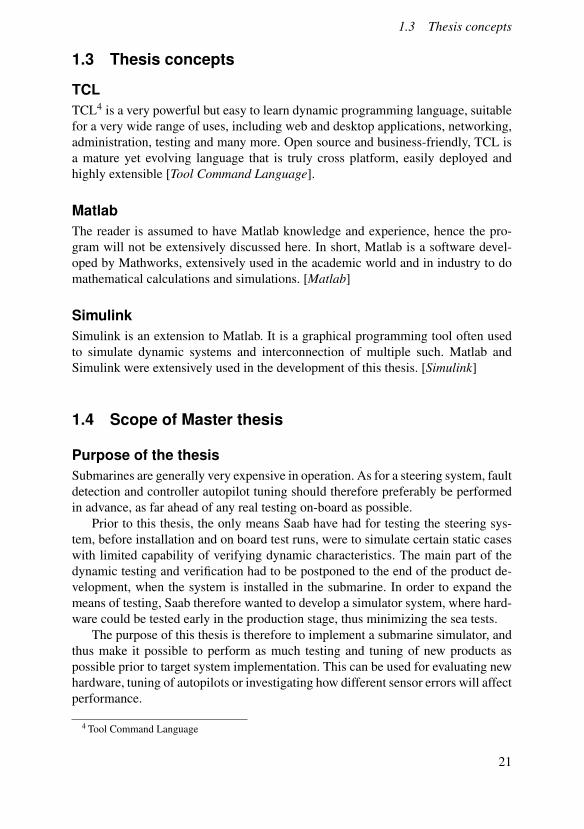
1.3 Thesis concepts

TCLTCL4 is a very powerful but easy to learn dynamic programming language, suitablefor a very wide range of uses, including web and desktop applications, networking,administration, testing and many more. Open source and business-friendly, TCL isa mature yet evolving language that is truly cross platform, easily deployed andhighly extensible [Tool Command Language].

MatlabThe reader is assumed to have Matlab knowledge and experience, hence the pro-gram will not be extensively discussed here. In short, Matlab is a software devel-oped by Mathworks, extensively used in the academic world and in industry to domathematical calculations and simulations. [Matlab]

SimulinkSimulink is an extension to Matlab. It is a graphical programming tool often usedto simulate dynamic systems and interconnection of multiple such. Matlab andSimulink were extensively used in the development of this thesis. [Simulink]

1.4 Scope of Master thesis

Purpose of the thesisSubmarines are generally very expensive in operation. As for a steering system, faultdetection and controller autopilot tuning should therefore preferably be performedin advance, as far ahead of any real testing on-board as possible.

Prior to this thesis, the only means Saab have had for testing the steering sys-tem, before installation and on board test runs, were to simulate certain static caseswith limited capability of verifying dynamic characteristics. The main part of thedynamic testing and verification had to be postponed to the end of the product de-velopment, when the system is installed in the submarine. In order to expand themeans of testing, Saab therefore wanted to develop a simulator system, where hard-ware could be tested early in the production stage, thus minimizing the sea tests.

The purpose of this thesis is therefore to implement a submarine simulator, andthus make it possible to perform as much testing and tuning of new products aspossible prior to target system implementation. This can be used for evaluating newhardware, tuning of autopilots or investigating how different sensor errors will affectperformance.

4 Tool Command Language

21


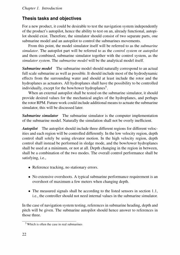
Thesis tasks and objectives

For a new product, it could be desirable to test the navigation system independentlyof the product’s autopilot, hence the ability to test on an, already functional, autopi-lot should exist. Therefore, the simulator should consist of two separate parts, onesubmarine model and an autopilot to control the submarines movements.

From this point, the model simulator itself will be referred to as the submarinesimulator. The autopilot part will be referred to as the control system or autopilotand them combined, submarine simulator together with the control system, as thesimulator system. The submarine model will be the analytical model itself.

Submarine model The submarine model should naturally correspond to an actualfull scale submarine as well as possible. It should include most of the hydrodynamiceffects from the surrounding water and should at least include the rotor and thehydroplanes as actuators. All hydroplanes shall have the possibility to be controlledindividually, except for the bow/tower hydroplanes5.

When an external autopilot shall be tested on the submarine simulator, it shouldprovide desired values for the mechanical angles of the hydroplanes, and perhapsthe rotor RPM. Future work could include additional means to actuate the submarinesimulator, this will be discussed later.

Submarine simulator The submarine simulator is the computer implementationof the submarine model. Naturally the simulation shall not be overly inefficient.

Autopilot The autopilot should include three different regions for different veloc-ities and each region will be controlled differently. In the low velocity region, depthcontrol shall solely be using elevator motion. In the high velocity region, depthcontrol shall instead be performed in sledge mode, and the bow/tower hydroplanesshall be used at a minimum, or not at all. Depth changing in the region in between,shall be a combination of the two modes. The overall control performance shall besatisfying, i.e.,

• Reference tracking, no stationary errors.

• No extensive overshoots. A typical submarine performance requirement is anovershoot of maximum a few meters when changing depth.

• The measured signals shall be according to the listed sensors in section 1.1,i.e., the controller should not need internal values in the submarine simulator.

In the case of navigation system testing, references in submarine heading, depth andpitch will be given. The submarine autopilot should hence answer to references inthose three.

5 Which is often the case in real submarines

22

1.4 Scope of Master thesis

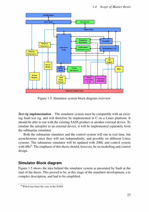
Figure 1.5: Simulator system block diagram overview.

Test rig implementation The simulator system must be compatible with an exist-ing Saab test rig, and will therefore be implemented in C on a Linux platform. Itshould be able to run with the existing SASS product or another external device. Toemulate the autopilot as an external device, it will be implemented separately fromthe submarine simulator.

Both the submarine simulator and the control system will run in real time, butasynchronous since they will run independently, and possibly on different Linuxsystems. The submarine simulator will be updated with 20Hz and control systemwith 4Hz6. The emphasis of this thesis should, however, be on modelling and controldesign.

Simulator Block diagramFigure 1.5 shows the idea behind the simulator system as presented by Saab at thestart of the thesis. This proved to be, at this stage of the simulator development, a tocomplex description, and had to be simplified.

6 Which has been the case in the SASS

23


Delimitation

The following delimitations will be assumed:

• Completely submerged submarine.

• The submarine will be in an infinitely large ocean to avoid near surface andnear bottom effects.

• No wave effects or irregular currents.

• Ideal sensors, i.e., measured value equals true value.

• Limited speed range, 4-16 knots.

• Incompressible hull.

• No tank systems (water pumping) will be modeled.

With these delimitation, Figure 1.5 could be simplified to Figure 1.6. The controlpart has been separated from the simulator itself, communication between them isnow through the data and control layer. The sea current in Figure 1.6 is limitedto constant currents that will only affect position/velocity relative earth. Also thesensor models have been removed as well as the submarine water tank actuators.The servo controllers for the hydroplanes and the propulsion will not be modeled ascontrol loops, but rather dynamics systems with unity gain.

1.5 Individual contribution

The the physical modelling and the model implementation in Simulink was per-formed by Erik Lind. Magnus Meijer was responsible for porting the model into Ccode and, hence, the model and controller interaction in the C environment. Magnusalso worked together with a consult as Saab to interface the thesis implementationwith the existing program structure in the test rig. The controller was designed byErik, but the dimensioning and weighting was performed by Magnus.

The introduction, development, and method chapters were written by Erik. Mag-nus wrote the theory, result, and discussion chapters.

1.6 Thesis Outline

This report consists of five Chapters, and can be summarized as follows:

Method In Chapter 2, the methods and the coordinate system notations and struc-tures used, will be presented. This Chapter will also explain how the model wasimplemented in Matlab and ported to the target language C.

24

1.6 Thesis Outline

Figure 1.6: Tuned down simulator block diagram.

Theory Chapter 3 consists of theory and background of hydrodynamics and somehydrodynamic modeling. After this, equations for a six degrees of freedom dynamicbody will be derived and, finally, a short collection of control designs and strategieswill be presented.

Development Firstly, Chapter 4 will explain how the known hydrodynamic rela-tions were applied to submarines, and how a model for a generic submarine modelcan be derived. This is followed by an introduction to a demo submarine, Finally,Chapter 4 will consist of the complete control system derivation.

Results / Simulation Chapter 5 presents the final model and autopilot, as well asplots from different simulated manoeuvres.

Discussion / Summary Chapter 6 consists of a discussion of the submarine modeland control system performance. The controller itself is also analyzed, with possibleoscillation and other issues. At last, ideas for future work is presented.

25

2Method

2.1 Coordinate System notation

This thesis will deal with numerous different coordinate systems. In this section, thesub- and superscript notation will be shortly described.

Positions, velocities and acceleration in (x,y,z) are denoted x,v, and a respec-tively. For increased clarity what a vector describes and in what coordinate systemit is currently expressed, sub- and superscripts will be added. Generally, vectors willbe written:

xABC (2.1)

where x is a vector, in this case a position vector. It could also be a velocity oracceleration vector. A is always a coordinate system abbreviation while B and C arepoints or coordinate systems (in such case the point will be the coordinate systemorigin). Equation (2.1) will thus describe the vector from point B to C expressed inthe coordinate system A. For example, let A and B be two coordinate systems, xB

AB isthen the position of OB relative OA expressed in the coordinates of B. And similarly,aB

AB is the acceleration of OB relative OA expressed in the coordinates of B, whichcan also be expressed as −aB

BA, etc.As for angle vectors (φ ,θ ,ψ) (roll, pitch, yaw), they are defined as the rotation

between two coordinate systems. Figure 2.1 describes the rotation of the blue framewith respect to the black frame. The rotations are defined in the order: yaw, pitch,and roll.

2.2 Simulator development

Matlab/ SimulinkThe submarine simulator and the control system will both be implemented andtested in Matlab/Simulink due to the many advantages these software provides forthis kind of task. The Simulink implementation will then be ported to C code, whichis already supported. Read more about porting Simulink models to C code below.

26

2.2 Simulator development

Figure 2.1: Coordinate system rotation definition, defined in the order: yaw, pitch,roll.

Figure 2.2: Test rig communication overview, with a SASS.

The controller and model simulator will not be updated simultaneously (20Hzvs 4Hz). Since Simulink does not support different step lengths in the same model,the dynamic parts of the controller were chosen to be implemented in discrete timeto simplify the simulation in Simulink.

CommunicationThe idea of the final implementation structure in the test rig is illustrated in Figure2.2. All the parts are connected through a data layer. The test operator will commu-nicate with the submarine simulator with telnet through TCL.

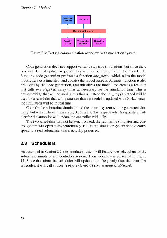
If the test system is a navigation system, the test rig setup should look morelike in Figure 2.3. The SASS has been replaced by a navigation system, and an au-topilot has been connected. The test operator will communicate with the submarinesimulator and autopilot in the same fashion as above. Communication between theautopilot and submarine simulator will be through TCP.

Code generation

Simulink features code generation for models, which produces C code that exactlyrepresents the model simulation. If the model has inputs and outputs, they will ap-pear as C structs in the generated code. There is also a feature to save the simulationoutput as a .mat file, which will be used to log data.

27

Chapter 2. Method

Figure 2.3: Test rig communication overview, with navigation system.

Code generation does not support variable step size simulations, but since thereis a well defined update frequency, this will not be a problem. In the C code, theSimulink code generation produces a function one_step(), which takes the modelinputs, iterates a time step, and updates the model outputs. A main() function is alsoproduced by the code generation, that initializes the model and creates a for-loopthat calls one_step() as many times as necessary for the simulation time. This isnot something that will be used in this thesis, instead the one_step() method will beused by a scheduler that will guarantee that the model is updated with 20Hz, hence,the simulation will be in real time.

Code for the submarine simulator and the control system will be generated sim-ilarly, but with different time steps, 0.05s and 0.25s respectively. A separate sched-uler for the autopilot will update the controller with 4Hz.

The two schedulers will not be synchronized, the submarine simulator and con-trol system will operate asynchronously. But as the simulator system should corre-spond to a real submarine, this is actually preferred.

2.3 Schedulers

As described in Section 2.2, the simulator system will feature two schedulers for thesubmarine simulator and controller system. Their workflow is presented in Figure??. Since the submarine scheduler will update more frequently than the controllerscheduler, it will call subonestep()eveni f noTCPconnectionisestablished.

28

3Theory

3.1 Hydrodynamics

Hydrodynamics is the study of liquids in motion. A body traveling through a fluidwill be exerted to a number of forces and moments, which is a result due to thephysical characteristics of the liquid medium. In this section some of the differenteffects will be discussed and shortly explained in general, i.e., not explicitly forsubmarines.

Hydrostatics

Archimedes’ principle states that a submerged body will experience a lifting forceequal to the gravitational force of the displaced water. This force will act through thecenter of buoyancy [Fossen, 1994], which is the center of gravity of the displacedwater, hence, this force is usually referred to as the buoyancy force. The gravityand buoyancy force will always be opposite in direction, which will cause the bodyto strive towards balance, i.e., when the center of buoyancy is vertically alignedwith the center of gravity (Figure 3.1). The magnitudinal difference between the twoforces will determine if the body will sink or float.

Figure 3.1: Buoyancy and gravity force.

29

Chapter 3. Theory

Figure 3.2: Turbulent and laminar flow.

Hydrodynamic DampingA body traveling through a fluid will experience a drag force parallel to the incom-ing flow, known as hydrodynamic damping. This force is a result from numerouseffects and are divided differently throughout literature and previous work. Thisthesis will divide the forces according to [Fossen, 1994] and [Fossen, 2011].

Pressure Drag Pressure drag is the force normally thought of as drag. As a bodytravels through water, it has to suppress liquid at the front in order to move forward.This is largely dependent on the shape of the body, a more streamlined body willexperience less pressure drag.

A common way to interpret this is to view it as a pressure difference. At thefront, where fluid is displaced to make room for the body, there will be an increasedpressure. At the aft, the fluid will be replaced into the space the body left behind, thepressure instead will be lower. This pressure difference will induce a force, similarto a airplane wing or sail lifting forces. A less streamlined aft will also create tur-bulence which will further decrease the pressure at the aft and thus further increasethe drag force.

Friction Drag Friction drag arises from friction between the body and the sur-rounding fluid. When a body travels through water, it will accelerate the fluid clos-est to its surface. This flow can be seen as parallel layers of fluid with friction inbetween. This will cause the different layers to have different velocities, decreasingwith the distance from the body, as seen in Figure 3.2.

The flow may be laminar or turbulent, or a combination of the both. Laminarflow is when there is no disruption between the parallel layers flowing past the body.This occurs at low velocities and gives rise to very low friction and noise. As thevelocity increases the different layers of fluid overturns and causes turbulence, seeFigure 3.2. This is very energy consuming, and causes high friction and noise.

Wave Damping Wave damping is the resistance experienced by the body whenadvancing through waves on the surface. This effect is the most important dampingcontributor in rough seas, due to the fact that the forces from the waves are pro-portional to the square of the wave height [Fossen, 2011]. This effect is neglectedin this thesis due to the delimitation presented in Section 1.4, i.e., the body will be

30

3.1 Hydrodynamics

completely submerged at a great depth, and therefore not affected by surface waves.

Potential Damping Potential damping refers to the energy loss when a body isforced to oscillate up and down with the surface waves. Due to the same reasons asfor wave damping, this effects is not taken into account in this thesis.

Drag coefficientThe effects of drag, at a certain velocity, is usually described by a non-dimensionaldrag coefficient, defined as:

Cd =−F

12 ·ρ ·A ·u2

(3.1)

where F is the drag force, ρ is the density of the fluid, A is the area shown to theflow and u the velocity of the body. For certain applications it is more common tonormalize with the area of the submerged hull, referred to as the wetted surface. Ina velocity interval, the drag coefficient is only marginally changing and Equation(3.1) can instead be used to calculate the resistance for a given velocity:

F =−Cd ·12·ρ ·A ·u2 (3.2)

Reynolds number Reynolds number is the relation between the inertial- and theviscous forces of a fluid. It is defined in open sea situations as [Fossen, 2011]:

Rn =uDν

(3.3)

where D is the characteristic length of body, u is the velocity and ν is the kinematicviscosity coefficient of the fluid. A high Reynold’s number means the flow is mainlyturbulent, while a lower generally corresponds to a more laminar flow.

Lift When an object is traveling through a medium, it will experience lift forcesperpendicular to the incoming flow. This effect is caused by pressure changes be-tween the top and bottom surfaces. The classical example is an airfoil travelingthrough air, see Figure 3.3. When the air is deflected it will have to travel aroundthe airfoil. Since the air above the wing will have to travel further than the air be-low, the pressure will decrease on the top surface, and create a lift force on theairfoil.

The lift generated is highly dependent on the angle of attack, i.e. the angle of thevelocity vector of the incoming flow. A perfectly symmetrical airfoil will produce nolift if the angle of attack is zero, but if it is tilted, there will be a pressure differenceand a lift force is generated.

All bodies moving through a medium will experience this effect. The hydroplanescan be compared with airfoils and will produce a great amount of lift when actuated.When manoeuvring the submarine, the incoming flow will change, and thus thesubmarine tower and hull will also generate lift forces.

31

Chapter 3. Theory

Figure 3.3: Flow past an airfoil.

Added mass When a body travels through water, the hull friction will acceleratethe water closest to the hull, creating a layer of moving water. The closest layer willin turn accelerate the next layer of water and so on. Hence, there will be an regionof moving water around the body.

When the body accelerates, it will also have to accelerate the water closest tothe hull. When it turns, it will have to turn the water that is traveling with the body.This effect is called the added mass effect since the body will appear heavier than itis. This will effect both the apparent mass and inertia of the body.

The added mass effect does also affect bodies moving through the air, but sincethe mass of the accelerated air is often negligible compared to the body mass, thisis rarely accounted for. The accelerated water, however, does have a considerablemass and will have to be taken into account when modelling bodies in water.

It is difficult to calculate how large this effect will be, since it heavily dependson the shape and roughness of the submarine, it is therefore usually analyzed withexperiments.

Control SurfacesTo be able to control the attitude of a submarine, several control surfaces are usedas described in Section 1.1.

Hydrodynamic Forces A hydroplane will both experience a drag force oppositeto the direction of the incoming flow, and a lift force perpendicular to it. [Toxopeus,2011] proposes a way to calculate the drag and lift forces, Dru and Lru, see Figure3.4,

Lru =12·ρ ·V 2

r ·AR ·Cl · cosδe · sinδe (3.4)

Dru =12·ρ ·V 2

r ·AR ·Cd · sin2δe (3.5)

where Vr is the velocity of the inflowing water, AR is the area of the rudder, Cl isthe lift coefficient, δe is the so called effective rudder angle, and Cd is the dragcoefficient. [Toxopeus, 2011] defines two angles, the hydrodynamic rudder angle,δh and the effective rudder angle δe. δh is the angle between the ship longitudinalaxis and the incoming flow, the effective rudder angle δe is the angle between themechanical rudder angle δ and δh, see Equation (3.6). As the name suggests, δe is

32

3.1 Hydrodynamics

Figure 3.4: Rudder forces according to [Toxopeus, 2011]. Note that Dru is oppositethe direction of the incoming flow, and that Lru is perpendicular to it

the rudder angle for which a force is generated, i.e., when δe is zero, no force iscreated.

δe = δ −δh (3.6)

In equation (3.6), δh = arctan( vyvx) where vy and vx are the x and y components of

the water velocity at the rudder. This translates to the body longitudinal and lateralforces and yaw moment:

Fx =−Dru · cosδh−Lru · sinδh (3.7)

Fy = Lru · cosδh−Dru · sinδh (3.8)

τ = x× (Fx,Fy,0) (3.9)

where x is the position of the rudder. The rudder drag and lift coefficients are usu-ally experimentally determined, but [Toxopeus, 2011] refers to previously derivedempiric formulas for calculating them.

Cl =6.13 ·Λ

2.25+Λ(3.10)

Cd =C2

lπ ·Λ

(3.11)

where Cl is the lift coefficient, Cd the drag coefficient, and Λ the so called rudderaspect ratio, Λ = length

area .

33

Chapter 3. Theory

Flow Straightening When a submarine is moving, the water flow vortex along thehull will alter the water flow at the rudders. [Toxopeus, 2011] suggests a methodto compensate for this phenomena by adding a flow straightening coefficient forthe hydrodynamic rudder angle δh, i.e., decreasing it. This will be neglected in thisthesis.

Flow straightening is enhanced by the propeller, greatly so when it is placed infront of the rudders. Although, for modern submarines, propellers are most oftenplaced behind the hydroplanes, in order to decrease noisy turbulence around therudders.

PropulsionThe propeller converts rotational motion into forward/backward thrust. To calcu-late the thrust Fp and torque τp, [Toxopeus, 2011] and [Watt, 2007] among others,suggests calculating dimensionless thrust and torque coefficients which only dependon the advance ratio J:

Kt(J) =Fp

ρn2D4p

(3.12)

Kq(J) =τp

ρn2D5p

(3.13)

J =vp

nDp(3.14)

where Fp is the force exerted by the propeller, τp is the torque generated, n is theRPS1, Dp is the diameter of the propeller, and vp is the velocity of the incoming flow.The functions Kt(J) and Kq(J) are determined by water tests or advanced computercalculations, when the propeller is operating at different advance ratios. Equation(3.12) and (3.13) can then be used for determining the thrust and torque.

Fp = Kt ·ρn2D4p (3.15)

τp = Kq ·ρn2D5p (3.16)

The propeller on a submarine is operating in a wake from the hull which reducesthe average inflow to the propeller. This is usually corrected with a one-dimensionalcorrection factor wT : [Toxopeus, 2011]:

vp = (1−wT ) ·u (3.17)

where wT if the so called Taylor wake fraction, and u the forward velocity of thesubmarine. Since the propeller accelerates water backwards, it generates a nega-tive pressure on the hull upstream from its position. This will increase the drag force

1 Revolutions Per Second

34

3.2 6 degrees of freedom dynamics

on the hull, negating some of the propeller thrust. This can be corrected with an-other constant, also suggested by [Toxopeus, 2011], known as the thrust deductionfraction t:

Fres = (1− t) ·Fp (3.18)

To determine wT and t, model experiments must be performed on the hull aloneto determine the wake fraction, as well as the hull with the propeller attached todetermine the thrust deduction factor.

Cavitation Cavitation is caused when forces acting on a liquid forms small cav-ities or bubbles. This is usually a result of rapid pressure changes, for examplearound a propeller. If the small cavities implode, they will generate an intenseshockwave. This is an undesired behaviour since repeated implosions are noisy andcauses heavy wear on materials.

3.2 6 degrees of freedom dynamics

A rigid body’s movement and position in a three dimensional space can uniquelybe described using six states. Its position can be determined with Cartesian (x,y,z)coordinates, and its turn by three angles (φ ,θ ,ψ) (which are the rotations aroundthe x-,y- and z- axes respectively). These six coordinates result in a system with sixdegrees of freedom. In this section the dynamics of such a system will be derived.

Consider a space-fixed coordinate system W and a body-fixed frame REF withthe origins OW and OR respectively. Let aG be the acceleration and xG the positionof the the center of mass. Let v be the velocity and ω the angular velocity of ORexpressed in the body-fixed coordinates REF. The acceleration aG is given by theNewton-Euler equations from classic mechanics: [Fossen and Fjellstad, 1995]

aG =∂v∂ t

+ω× v+ ω×xG +ω× (ω× xG) (3.19)

In order to simplify the readability of Equation (3.19) the standard vector notationwas circumvented and will instead be presented in Table 3.1.

With forces (Fx,Fy,Fz)i acting on the origin OR, the movement of the body willbe:

∑(Fx,Fy,Fz)i = maG (3.20)

where m is the mass.Angular momentums τ i around OR results in the movements:

∑τ i = Jω +ω×Jω +xG×aG (3.21)

where J is the moment of inertia matrix. Equations (3.19) and (3.21) will be com-bined, i.e., substitute aG from (3.19) in (3.21), to create the angular acceleration.

35

Chapter 3. Theory

xG xRRG

aG aRRG

v vRWR

ω ωRWR

Table 3.1: The vectors in Section 3.2 written with the standard notation

3.3 Control designs

In this Section a very short summary of a few different control designs used in thisthesis are discussed. For more information, see [Glad and Ljung, 2003].

PID

The PID-controller is the most common type of feedback controller throughout in-dustry. It consists of three parts, the proportional part P, the integral part I, andthe derivative part D. The controller tries to minimize the control error, that is, thedifference between a desired setpoint and the measured output of the process. ThePID-controller output u(t) is defined as2.

u(t) = Kp · e(t)+Ki ·∫ t

0e(τ)dτ +Kd ·

ddt

e(t) (3.22)

where Kp, Ki and Kd are the tunable gain parameters for the proportional, integralrespective the derivative parts and e(t) = r(t)− y(t), is the control error.

PID Tracking Switching between multiple PIDs in a controller system is not un-common. The different controllers are most certainly dimensioned differently, hence,the control signal will suffer a step at the time of the switch. In order to avoid be-haviour like this, it is possible to implement PID tracking, where the non active con-trollers follow the output of the active one. PID tracking is implemented in Simulinkas in Figure 3.5

State FeedbackA system on standard state space form is written as in Equation 3.23.

x = Ax+Buy = Cx+Du

(3.23)

When controlling a system on state space form, a popular control method is theso called state feedback control, where the control signal u is the state vector xmultiplied by a feedback gain matrix L. This allows the control engineer to place

2 This is the most basic of PID controller definitions, other variants do exist

36

3.3 Control designs

Figure 3.5: PID tracking implementation.

the closed loop poles freely in the s-plane3. This is desirable since the poles greatlyinfluence the response of a system.

The poles of an open loop system are given by the roots of characteristic equa-tion |sI−A|= 0. With state feedback, the control signal u takes the form u =−Lx,the system in Equation (3.23) can then be written as:

x = (A−BL)xy = (C−DL)x

(3.24)

The new characteristic equation

det(sI− (A−BL)) (3.25)

The new characteristic equation takes the form in Equation (3.24), where L is cho-sen to place the poles at the desired locations.

ObserverWhen using state feedback controllers for system control, all the states have to beknown. This is often not the case, since rarely all are measured. Some states mightnot even have a direct physical interpretation, which complicates measuring further.A state feedback controller therefore has to be complemented with an observer. Anobserver estimates the unknown states4 from the input to the system and the known(measured) output signals, and feeds them to the controller (Equation (3.26)).

˙x = Ax+Bu+K(y−Cx)u =−Lx

(3.26)

3 If the system is controllable.4 This is possible if the system is observable.

37

Chapter 3. Theory

where x is the observed state vector and K the observer gain matrix, which will bedimensioned to create the desired observer dynamics. A common way of doing this isby letting the observer gain matrix be a Kalman filter, which is an optimal observerwith respect to measurement noise and process disturbances5. As the name suggests,the Kalman filter is not only an observer, but a filter, that prevents measurementnoise to be fed back into the system.

Optimal control - LQGA method of dimensioning the state feedback control of a system, is by using LinearQuadratic Gaussian control theory. The idea of LQG is to minimize a quadratic costfunction, which will yield an optimized controller with respect to certain weights onthe controlled variables and control efforts:

min(||e||2Q + ||u||2R) = min∫

eT (t)Qe(t)+uT (t)Ru(t)dt (3.27)

where Q and R are the weight matrices for the error e(t) and control signal u(t).These are used to weigh the control effort against the control error, i.e., how topenalize the different control errors, and the different control signals.

To determine the optimal controller, the system is written on the general statespace form used in [Glad and Ljung, 2003]:

x = Ax+Bu+Nv1

z = Mxy = Cu+ v2

(3.28)

where v1 is a white Gaussian disturbance vector and z are the controlled variables.v2 is the measurement noise, also of white Gaussian characteristic. Consider thesystem above, where [ v1

v2 ] are stochastic noise with intensity[

R1 R12RT

12 R2

]. The sought

feedback, uFB =−Lx will minimize the expression [Glad and Ljung, 2003]:

||z||2Q + ||u||2R (3.29)

The feedforward control part uFF = Lrr will be dimensioned to ensure that theclosed loop gain is identity:

M(BL−A)B ·Lr = I (3.30)

The observer gain matrix K will create the perfect trade off between the systemmodel and the measured output.

5 The Kalman filter assumes white Gaussian noise and disturbances.

38

4Development

4.1 Modelling of a submarine

The dynamics of a body with six degrees of freedom where presented in Section 3.2.This Section will apply those equations to a submarine submerged in water and tryto model the external forces Fi = (Fx,Fy,Fy,τx,τy,τz)i which are hydro-static andhydro-dynamic forces and torques, as well as propulsion and hydroplane forces andmoments.

Coordinate Systems and notationThe following coordinate systems will be extensively used:

Name abbr.1 subs.2 explanation x,y,z corresponds toLon/lat LL L Earth fixed longitude, latitude,

depthWater W W Water fixed north, east, downReference REF R Body fixed in the

center of buoyancybow, starboard, down

Center of gravity G G - bow, starboard,downxR

RG = (xG,yG,zG)

Earth frame A position in LL is given by (longitude, latitude, depth), which willbe denoted by (x,y,z)L.

Water frame The (x,y,z)W axes corresponds to (north, east, down)-directions. Theorigin of W moves with the water currents which means that the relation between Wand LL is a simple translation in the (x,y)L- plane that varies with time.

1 abbreviation2 subscripts

39

Chapter 4. Development

Figure 4.1: Reference frame velocity notation.

Reference frame The REF frame is submarine-fixed and the origin is placed in thecenter of buoyancy. This is preferable since the center of buoyancy rarely changeswhile the center of gravity depend on load and the condition of the different tanks. Asfor the REF coordinate system, the axes will be denoted (x,y,z)R and the velocitiesaccording to the standard convention used in literature3 (u,v,w), i.e. (x, y, z)R

WR, and(p,q,r) for the angular velocities, see Figure 4.1. For the forces and moments, F =(Fx,Fy,Fy,τx,τy,τz)

RWR = (X ,Y,Z,K,M,N) will be used, as is also the standard.

The relation between (p,q,r) and (φ , θ , ψ) are:

φ = p+qsinφ tanθ + r cosφ tanθ

θ = qcosφ − r sinφ

ψ = qsinφ

cosθ+ r

cosφ

cosθ

(4.1)

Submarine six degrees of freedomThe W and REF frames in Section 3.2 will indeed be the water and body frames.With this notation, Equation (3.20) and (3.21) correspond to:

m(u− vr+wq− xG(q2 + r2)+ yG(pq− r)+ zG(pr+ q)) = ∑Xi (4.2a)

m(v−wp+ur− yG(r2 + p2)+ zG(qr− p)+ xG(qp+ r)) = ∑Yi (4.2b)

m(w−uq+ vp− zG(p2 +q2)+ xG(rp− q)+ yG(rq+ p)) = ∑Zi (4.2c)

Ix p+(Iz− Iy)qr− (r+ pq)Izx +(r2−q2)Iyz +(pr− q)Ixy = ∑Ki (4.2d)

Iyq+(Ix− Iz)rp− (p+qr)Ixy +(p2− r2)Izx +(qp− r)Iyz = ∑Mi (4.2e)

Izr+(Iy− Ix)pq− (q+ rp)Iyz +(q2− p2)Ixy +(rq− p)Izx = ∑Ni (4.2f)

3 defined by SNAME (1950)

40


The Equations (4.2) are nonlinear and quite complex, neither do they explicitlystate expressions for (u, v, w, p, q, r). However, Equations (4.2) are linear in sense of(u, v, w, p, q, r) and can thus be solved by a matrix inversion. Modeling a submarineis now divided into modeling the different forces and moments in the 6 directions.

External ForcesThe effects and forces from Section 3.1 are summarized as:

∑Fi = FHS +FHD +FP +FC (4.3)

where FHS are the hydrostatic forces and moments, i.e., gravity and buoyancyforces, FHD are the hydrodynamic forces from added mass and inertia, drag andcross flow, FP are the propulsion forces, and FC are forces from the control sur-faces, i.e., the different hydroplanes. The forces and moments are now collected inthe Equations (4.4).

∑Xi = XHS +XHD +XP +XC (4.4a)

∑Yi = YHS +YHD +YC (4.4b)

∑Zi = ZHS +ZHD +ZC (4.4c)

∑Ki = KHS +KHD +KP +KC (4.4d)

∑Mi = MHS +MHD +MC (4.4e)

∑Ni = NHS +NHD +NC (4.4f)

This is a common way of interpreting and dividing forces acting on a submarinein papers and literature. The extra terms in the xR- direction and rotation aboutthe xR- axis are due to the propulsion and induced torque from the propeller. Thisassumes that, that the rotor is perfectly aligned with the center of buoyancy xR

RB inthe (y,z)R- plane which is rarely true. More accurate would be to also introduce apitch moment due to rotor propulsion, however, this lever arm would probably besmall and therefore, this effect is therefore not accounted for.

Hydrostatic forcesFor a 6 DOF body, the hydrostatic forces in Section 3.1 are calculated as: [Feldman,1979].

XHSYHSZHSKHSMHSNHS

=

−(W −B)sinθ

(W −B)cosθ sinφ

(W −B)cosθ cosφ

(yGW − yB)cosθ cosφ − (zGW − zBB)cosθ sinφ

−(xGW − xBB)cosθ cosφ − (zGW − zBB)sinθ

(xGW − xBB)cosθ sinφ − (yGW − yBB)sinθ

(4.5)

where W is the gravity force and B is the buoyancy force.

41


Hydrodynamic derivativesHydrodynamics is a very complex phenomena and physically very hard to model.Most of the formulas derived are empirical and they should thus be used with cer-tain care. Many authors deal with the subject of hydrodynamics by replacing FHDwith a coefficient based model, with terms like Xu|u|u|u|, cross terms like Xuyuy andderivative terms like Xuu or Xqq. For example. the forces in xR- direction could looksomething like this: [Ridley et al., 2003]

∑Xi =XHS +XP +XC +Xu|u|u|u|+Xuu+Xuvuv+Xvwvw+Xv|v|v|v|+Xvrvr+Xw|w|v|w|+Xwqwq+Xqqqq+Xrrrr

(4.6)

The equations for (X ,Y,Z,K,M,N)i differ slightly throughout previous works. Xu|u|and Xv|v| describes how movement in X- and Y- direction creates a longitudinalforce, which will be relative to the signs of u and v. Xu is the induced force in xR-direction due to acceleration. Xuv describes a force along xR due to combined u andv movement. Similarly, Xvw models how a combined movement in v and w createsa force in xR- direction etc. The terms including an absolute value of a velocity isinterpreted as a drag term, since they are quadratic and relative to the direction. Thederivative subscript terms, e.g., Xu, try to model the apparent increased mass dueto water acceleration around the hull, as described in Section 3.1. The cross terms,e.g., Xuv, are forces from combined movements in different directions which arisedue to the accelerated water around the hull. The sum of the different terms canbe seen as a Taylor expansion and the coefficients are often called hydrodynamicderivatives, i.e.:

Xu =∂X∂ u

(4.7)

Because of this, one could of course model a submarine with a Taylor expansionof higher order. However, this is unusual in previous works in this subject in orderto avoid unwanted behaviour to far from the operating point, i.e., outside someinterval of validity. The reader will probably notice that the Taylor expansion inEquation (4.6) does not include all the possible combinations of (u,v,w, p,q,r), thisis because some are considered zero, or at least small, which will be shown.

The added mass terms add additional u, v, ..., r terms to Equation (4.2), whichare collected into the symmetric added mass matrix [Fossen, 2011]:

FHD =

Xu Xv Xw Xp Xq XrYu Yv Yw Yp Yq YrZu Zv Zw Zp Zq ZrKu Kv Kw Kp Kq KrMu Mv Mw Mp Mq MrNu Nv Nw Np Nq Nr

uvwpqr

+ ... (4.8)

42


Rearranging Equation (4.2) with only derivative terms on the left hand side yields:m 0 0 0 mzG −myG0 m 0 −mzG 0 mxG0 0 m myG −mxG 00 −mzG myG Ix −Ixy −Izx

mzG 0 −mxG −Ixy Iy −Iyz−myG mxG 0 −Izx −Iyz Iz

uvwpqr

= ... (4.9)

Moving the added mass term in Equation (4.8) to the left hand side and combiningwith Equation (4.9) gives:

m−Xu −Xv −Xw −Xp mzG−Xq −myG−Xr−Yu m−Yv −Yw −mzG−Yp −Yq mxG−Yr−Zu −Zv m−Zw myG−Zp −mxG−Zq −Zr−Ku −mzG−Kv myG−Kw Ix−Kp −Ixy−Kq −Izx−Kr

mzG−Mu −Mv −mxG−Mw −Ixy−Mp Iy−Mq −Iyz−Mr−myG−Nu mxG−Nv −Nw −Izx−Np −Iyz−Nq Iz−Nr

(4.10)

which is the so called mass matrix, which will be denoted M. Since the submarineaccelerates water around its hull, the apparent mass will increase which meansthat at least the diagonal elements of Equation (4.8) should be negative, in order toincrease the diagonal elements in Equation (4.10).

Due to hull symmetry, many of these added mass coefficients are zero. For sub-marines, it is common to assume symmetry about the xz- plane which leads to thefollowing terms being zero, some of these due to symmetry in the added mass matrix[Watt, 2007]

Xv,Xp,Xr,Yu,Yw,Yq,Zw,Zp,Zq,Ku,Kw,Kq,Mv,Mq,Mr,Nu,Nw,Nq = 0 (4.11)

Determine hydrodynamic coefficientsModel testing A common method of determining hydrodynamics coefficients is toexperiment on a small replica of the vessel in a laboratory pool. This method can beconsidered to be the most accurate since there are no assumptions or simplificationsinvolved. The coefficients derived for the model will then be scaled to fit a full scale.These coefficients may be accurate for the model, but some accuracy is lost due tononlinearity in the equations, and non scaling water viscosity [Larsson and Raven,2010]. During the testing, the model is forced into certain manoeuvres and theforces on the hull are measured [Åström and Källström, 1976].

Real testing Another alternative is to derive the coefficient through actual fullscale testing, as previously done in [Åström and Källström, 1976], where the coef-ficients for a freighter and a tanker where derived through actual testing. An issuewith this is the cost, especially for submarines where the operating costs are huge.

43


As also pointed out by [Åström and Källström, 1976], for a full identification to bepossible, information about the motion in all the possible degrees of freedom is nec-essary. For a surface going vessel this means you need to measure, u, v, and r, andfor a submarine with 6 DOF you need to measure all the six movements u,v,r, p,w,and r for a proper system identification.

Computational fluid dynamics (CFD) Computational fluid dynamics, is thegeneric name for software used to simulate fluid motion and force on submergedor partly submerged bodies. They have not yet been fully accepted in the scientificcommunity and pool testing is still preferred when designing hulls. However, withincreased computational capacity in the every day computer, CFD softwares arebecoming more and more popular in prediction of ship motion. This can be seen bythe numerous reports in the last years where authors simulate ship motion or derivethe hydrodynamic coefficients through a CFD software, .e.g., [Toxopeus, 2011].

Prediction formulas Despite the lack of manageable analytic theory in the subjectof hydrodynamics, there do exist some partly analytic, partly empirical, formulas inpredicting added mass terms for submarines.

Ship manoeuvring forcesOne of the difficulties with hydrodynamic modelling, is to model hydrodynamicforces when turning, i.e., drifting. Hydrodynamics coefficients in steady state aresomewhat constant but when the state change, the water flow around the hullchanges direction and with that the hydrodynamic derivatives. As for the hull drag,a simple way of tackle this is to divide the flow into components and let the dragforce in the different directions act on the water’s relative inflow speed. That is, thedrag force in yR is a function of the sway v and the yaw r, and correspondingly,the force in the xR- direction is a function of the surge u. The problem with thismethod is that the inflowing water sees a different shape and effective area in caseof a drift, which means that the drag coefficients do in a way change with the angleof drift. A submarine will also be exerted to lift forces due to hull bound vortexeswhich is described in Section 3.1. Even more complex, typically for 6 degrees offreedom systems, is combined movement, e.g., a pitching movement while yawing.In the case of submarines, these motions will be handled separately as suggested by[Fossen, 2011], that is, the model will not explicitly account for combined yaw andpitch movements.

[Feldman, 1979] proposes a way to model hull drag by applying strip theory,i.e., split the hull in multiple sections and then, the drag force on a section will be afunction of the local velocity. For example the integral term in the YHD- expressionwith w = 0:

−ρ

2Cd

∫L

h(x)(v+ r · x)|v+ r · x|dx (4.12)

where h(x) is the local hull height and L is the hull length. Correspondingly, the

44


yaw moment due to a turning motion will be:

−ρ

2Cd

∫L

x ·h(x)(v+ r · x)|v+ r · x|dx (4.13)

Hydrodynamics in literature[Feldman, 1979] provides a complete notation and collection of the David W. Taylornaval ship research and development center standard equations of motion for sub-marines. These equations are widely quoted and referred to in submarine modellingpapers and is, according to FOI4, still the standard way of modelling underwatervehicles with six degrees of freedom. In addition to the hydrodynamic derivativeterms, Feldman includes integral terms to model drag while turning and flow vortexlift effects. These equations will be extensively used in this thesis.

[Humphreys and Watkinson, 1978] provides analytical expressions for approxi-mating added mass terms. This is done by collecting work from [Lamb, 1932] andapproximating the bare hull of a submarine as an ellipsoid. In addition, the paperincludes semi-empirical added mass and inertia effects due to the flow around thehydroplanes. Finally, the validity and problems with the formulas are discussed.

[Ridley et al., 2003] uses a simplified version of Feldman’s standard equationsto simulate a torpedo. The coefficients are derived through physical model testingin a pool. From Feldman’s equations the integral terms due to turning drag andhull vortexes are excluded. This is instead modeled by letting the force always bedirected opposite to the inflow of the water with a drag coefficient that increasesquadratically with the angle of attack and drift. The drag force is then divided intocomponents in the different directions and will serve as drag when the model isturning, i.e., drifting.

[Watt, 2007] uses a CFD software to derive the hydrodynamic derivatives for asubmarine computer model. However, he uses a distinct way of calculating the dragwhere coefficients are functions of the sway and heave drifts, e.g., the drag in xR-direction:

XD = Xuvw(u,v,w) · (√

u2 + v2 +w2)2 (4.14)

This is a way to model the change of flow around the hull while manoeuvring.[Toxopeus, 2011] simulates a number of surface vessels with the hydrodynamic

forces and moments computed through a CFD software, unlike the more commonway of a coefficient based prediction. He finds that this is a more accurate approachin simulating water going vessels.

[Fossen, 2011] and [Fossen, 1994] are extensive works that collects a great dealof the current knowledge in the subject of hydrodynamics. The author compiles anumber of different models that have been used in predicting ship motion throughwater over the years and refer to [Humphreys and Watkinson, 1978] for discussionand prediction of submarine hydrodynamic derivatives.

4 Totalförsvarets forskningsinstitut, (Swedish defence research agency)

45


4.2 Generic submarine model

In this Section a model for a generic submarine will be derived. The equations in[Feldman, 1979] will serve as a template. The hydrodynamic added mass terms willbe approximated according to [Humphreys and Watkinson, 1978].

As for the rudders, the equations proposed by [Toxopeus, 2011] will be used andmodified for three dimensions and for the rotor propulsion and torque, the model in[Watt, 2007] will be used.

Hydrodynamic derivativesThe hydrodynamic derivatives will be calculated by approximating the submarineas an ellipsoid. The hydroplanes are seen as flat plates as suggested by [Humphreysand Watkinson, 1978]. The added mass effect from the sail will be calculated byapproximating the sail as a huge hydroplane.

Cross flow dragThe cross flow drag was modelled according to [Feldman, 1979].

Y :− ρ

2Cd

∫L

h(x)v(x)√(w(x)2 + v(x)2)dx (4.15a)

Z :− ρ

2Cd

∫L

b(x)w(x)√(w(x)2 + v(x)2)dx (4.15b)

M :− ρ

2Cd

∫L

x ·b(x)w(x)√(w(x)2 + v(x)2)dx (4.15c)

N :− ρ

2Cd

∫L

x ·h(x)v(x)√(w(x)2 + v(x)2)dx (4.15d)

where b(x) and h(x) are the local width and heigh at x. w(x) and v(x) are the localvelocities at x:

v(x) = v+ r · xw(x) = w+q · x

(4.16)

Cd in (4.15) is the cross flow drag coefficient. For accurate prediction, Cd will haveto be specified separately for each Equation in (4.15). Since the hull has differentshape over the body, and the local velocities are different over the hull according toEquation (4.16), an even more accurate prediction will be to also let Cd be a functionof the position x and the local velocity.

When specifying a submarine model, the functions h(x) and b(x) will have tobe provided. When not specified, the model will use the value Cd = 1.19 for allequations in Equation (4.15) as suggested by [Hickey, 1990].

46


Figure 4.2: Rudder angles in three dimensions.

Control surfaces[Toxopeus, 2011] presents formulas for rudder forces and moments for a surfacegoing vessel. These equations, modified to fit three dimensions, will be presentedin this section. As described in Section 3.1, the formulas need the hydrodynamicrudder angle δh.

The water velocity vector at a rudder at the position xr (w/o hull and rotor ef-fects) is calculated in Equation (4.17).

vr =−(ν1 +ν2×xr) (4.17)

ν1 = (u,v,w)

ν2 = (p,q,r)(4.18)

This velocity will be projected on a plane orthogonal to the rudder, with normal N,see Figure 4.2.

Vre = (I− NNᵀ

NᵀN)Vr

5 (4.19)

Note that Vr and vr is the same vector, only that Vr is the vector expressed as acolumn matrix. δh will be the angle between Vre and [−1 0 0]ᵀ. The drag and liftforces Dru and Lru, are calculated according to Section 3.1. The direction for Druwill be the same as Vr. Lru will work in the direction N×Vr.

47


Each hydroplane will have a specific direction in which it operates, i.e., a normalrudder could have the direction (0,1,0) and a horizontal hydroplane could havethe direction of operation (0,0,1). As for an × configuration, the force directionscould be (0,±1/

√2,±1/

√2). Apart from that, the user will have to specify the

hydroplane positions xhp1−6, the hydroplane area and the lift and drag coefficientsCl and Cd . With this data, the lift and drag forces and moments for each hydroplaneare calculated.

An issue with the equations presented by [Toxopeus, 2011], is that they do notdeal with cross flow and coupled motion in 3 dimensions. For a + rudder config-uration and no combined pitch/yaw motion, this would not be a problem. But for× rudder configurations, the rudders will experience coupled motion even whencombined pitch/yaw motion is avoided.

Tower drag and liftAn attempt to model the tower lift and drag was done by using the same equationsas for the hydroplanes, applied to the tower dimension and position. It is difficult tostudy the validity of this method. The only validation performed, was to study thedirections of the forces, but not the magnitude. This suggest that this approximationshould not be used in a simulation before this method is verified. This will not befurther discussed.

Propeller propulsion and force

Equations for forces and torques created by the propeller, were presented in Section3.1, where XP and KP depend on the coefficients Kt and Kq, which in turn are func-tions of the advance ration J. These two coefficients depend heavily on the shapeof the propeller and have to be derived through actual testing or CFD calculations,which is outside the scope of this thesis. As for the generic model, the user hasto specify how Kt and Kq are functions of J. However, the model will provide asuggested relation according to previous works.

[Watt, 2007] presents two eighth-order polynomial interpolations for Kt and Kqas functions of the advance ratio J, derived through CFD calculations. Other rela-tions have been derived, e.g., by [Toxopeus, 2011], but [Watt, 2007] also deals withthe subject of submarines, hence, this was chosen. The coefficients Kt and Kq asfunctions of the RPS n at two different speeds are plotted in Figure 4.3. The in-terpolating polynomials can be found in Appendix A.1. The reader will probablynotice the RPS n in the denominator for the advance ratio, this function is there-fore not valid for close to zero RPS. At some points, Kt and Kq are negative, whichmean that the force/torque from the propeller is negative, which of course is notat all impossible, since slow RPS at high velocities could produce more drag thanpropulsion.

48


(a) Kt , u fixed. (b) Kq, u fixed.

(c) Kt , n fixed. (d) Kq, n fixed.

Figure 4.3: Kt(J) and Kq(J) relation.

Hydroplane dynamicsThe submarine model is manoeuvred by slanting the hydroplanes, i.e., specifyingmechanical angles δk. However, positioning the hydroplanes are control problemsthemselves. An accurate dynamic model description for the different hydroplanesis outside the scope of this thesis, although it could be desirable to include somehydroplane dynamics.

For the generic model, the positioning of the hydroplanes is approximated by asimple first order system where it is possible for the user to specify a time constantfor each control surface.

δk =1

s/Tk +1δre f k (4.20)

49


Figure 4.4: Submarine demo model.

Rotor dynamicsSimilarly to the hydroplanes, the rotor dynamics is approximated by a simple firstorder system with a user defined time constant.

n =1

s/T +1nre f (4.21)

4.3 Submarine demo model

During the literature study for this thesis, the authors came into contact with FOI.They confirmed the difficulties in modelling water crafts but provided a full modelof a demo submarine derived through CFD calculations of a CAD model of a sub-marine (Figure 4.4). The mathematical model was according to Feldman’s equa-tions. Table 4.1 shows the mechanical data for the demo submarine. The completeset of hydrodynamic coefficients can be found Section 6.1, and compared with thecoefficient derived from mechanical data according to the approximation methodby [Humphreys and Watkinson, 1978].

General features of the demo model Some general features of the demo subma-rine are presented in the list below.

6 Relative the aft of the submarine, expressed a as positive oriented orthonormal coordinate system(x,y,z) with z- axis upwards.

50

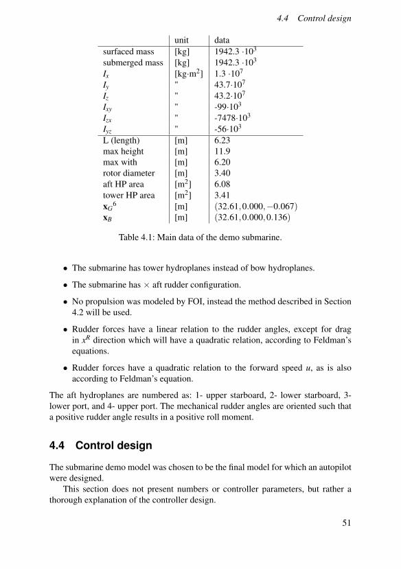
4.4 Control design

unit datasurfaced mass [kg] 1942.3 ·103

submerged mass [kg] 1942.3 ·103

Ix [kg·m2] 1.3 ·107

Iy " 43.7·107

Iz " 43.2·107

Ixy " -99·103

Izx " -7478·103

Iyz " -56·103

L (length) [m] 6.23max height [m] 11.9max with [m] 6.20rotor diameter [m] 3.40aft HP area [m2] 6.08tower HP area [m2] 3.41xG

6 [m] (32.61,0.000,−0.067)xB [m] (32.61,0.000,0.136)

Table 4.1: Main data of the demo submarine.

• The submarine has tower hydroplanes instead of bow hydroplanes.

• The submarine has × aft rudder configuration.

• No propulsion was modeled by FOI, instead the method described in Section4.2 will be used.

• Rudder forces have a linear relation to the rudder angles, except for dragin xR direction which will have a quadratic relation, according to Feldman’sequations.

• Rudder forces have a quadratic relation to the forward speed u, as is alsoaccording to Feldman’s equation.

The aft hydroplanes are numbered as: 1- upper starboard, 2- lower starboard, 3-lower port, and 4- upper port. The mechanical rudder angles are oriented such thata positive rudder angle results in a positive roll moment.

4.4 Control design

The submarine demo model was chosen to be the final model for which an autopilotwere designed.

This section does not present numbers or controller parameters, but rather athorough explanation of the controller design.

51


Model IOsThe control signals to the submarine at the current state7 are the requested hy-droplane positions and rotor RMS. The outputs are the signals measured by theINS and the control efforts, i.e. actual hydroplane positions and rotor RMS, seeFigure 4.5. The possibility to view the true states of the process will also exist forvalidation purposes.

Figure 4.5: Submarine simulator IOs.

Controller taskWith the controller requirements from Section 1.4, the final system should take theform as in Figure 4.6. Since there are no requirements for velocity control, thiswill not be included in this thesis, i.e., the control system’s means to actuate thesubmarine will be through the hydroplanes.

Figure 4.6: Simulator system IOs.

Controller hierarchy

The submarine has a number of different modes, but not all are required to follow areference. When linearized, the system was chosen to have the states x in Equation4.22.

x = [φ θ δ1 δ2 δ3 δ4 δ5 δ6 u v w p q r]ᵀ (4.22)7 Future work could include including the condition of the different tanks as control signals.

52

4.4 Control design

Figure 4.7: r, φ , θ controller.

Depth and heading are not included in the state vector. They do however have adynamic relation to the state vector. With zero roll (φ = 0), the change in depth canbe expressed as z=w−u ·sin(θ). In a sledge mode depth changing manoeuvre, w isnot accounted for, and for small θ the equation falls down to a first order integratorat a certain speed (u constant):

z = u ·θ (4.23)

As for the elevator depth changing manoeuvre, the pitch will stay zero and therelation becomes instead:

z = w (4.24)

With zero roll and pitch, the change in yaw will also be of first order integratorcharacteristics, ψ = r. The natural choice for a controller structure would then beto, at first, stabilize and control φ , θ , and r (Figure 4.7). With this, controlling thedepth and yaw becomes a simple task.

Inner controllerThe inner loop r, φ , θ -controller was chosen to be of LQ8 state feedback character-istic. An integrator for each controlled mode was added to remove stationary errorscaused by simulated stationary disturbances and model inaccuracies due to the lin-earization. The system on state space form becomes, with the notation in 3.3, as inEquation (4.25).

˙x = Ax+Bδ re f

z = Mx =

0 0 0 · · · 0 11 0 0 · · · 0 00 1 0 · · · 0 0

x(4.25)

In order to allow state feedback, an observer had to be added since only the INSand control effort signals can be measured. The final inner loop control structurecan be found in Figure 4.8.

8 Linear Quadratic Control, i.e., linear system with quadratic criteria

53


Figure 4.8: Inner loop controller structure.

State feedback The state feedback gain L was calculated with the Matlab com-mand lqry(sys,Q,R,N), which computes the optimal state feedback controller ofsystem sys with the weight function, see Section 3.3:

J = zᵀQ z+δᵀre f R δ re f + zᵀN δ re f (4.26)

State feed forward The feed forward gain Lr is given by Equation 3.3

[M(BL−A)B] ·Lr = I3×3 (4.27)

M(BL−A)B has the size 3×6, and Lr the size 6×3. Equation (4.27) is therefore anunderdetermined system of equations, i.e., we have a total of 18 unknown variablesbut only 9 equations. This was expected, since there are more than one way tooperate the hydroplanes to create a certain movement. In addition to this, a changein roll reference will probably never occur. This means that the second column inLr is of no interest. The second row of M(BL−A)B and the second column of Lrare therefore removed, and form Γ and Lr.

Γ · Lr = I2×2 (4.28)

The result is a system of equations with 12 unknown variables but only 4 equations.This meant that it was possible to add more constraints on the solution. To beginwith, there is no need for the bow/tower hydroplanes to answer to a reference changein r, which means Lr5,1 = Lr6,1 = 0. The bow/tower HPs are also often connected,i.e., Lr6,2 = Lr5,2. Equation (4.28) becomes:

Γ ·

Lr1,1 Lr1,2

Lr2,1 Lr2,2

Lr3,1 Lr3,2

Lr4,1 Lr4,2

0 Lr5,20 Lr5,2

=

[1 00 1

](4.29)

54

4.4 Control design

Equation (4.29) is still an underdetermined system of equations. Consider insteadthe optimization problem of solving (4.29) with the least possible control effort. TheHP angles δ at a reference change relate to the values in Lr. With Lr = [Lr1 Lr2],X =

[Lr1Lr2

]is defined.

minX

XᵀHX

s.t. Γ · Lr = I2×2

(4.30)

With H in Equation (4.30) it is possible to weigh certain HPs, to create the desiredreference tracking control. It is also possible to add additional constraints to theproblem (4.30), e.g., if one hydroplane has malfunctioned it is possible to add thisas a constraint to the optimization problem.

Observer The state feedback controller requires the state vectorx = [φ θ δ1 δ2 δ3 δ4 δ5 δ6 u v w p q r]ᵀ. From Section 1.1 the measured states couldinclude y = [φ θ δ1 δ2 δ3 δ4 δ5 δ6 u p q r]ᵀ. However, as for u, the observer wouldnaturally believe that u is constantly decreasing due to the rotor RPS is not includedas a model actuator. This would probably result in a stationary error in the log ve-locity u. To counter this, a new system model was derived for the observer where therotor RPS was included as a system actuator together with the hydroplane angles.To simplify the observer, the actual hydroplane angles and rotor RPS served as theinput signals since they were all measurable. This resulted in the state space systemin Equation (4.31) for the observer with the states x′ = [φ θ u v w p q r], and systemmatrices A′, B′, and C′.

˙x′ = A′x′+B′[

δ

n

]y′ =

[I3×3 03×2 03×303×3 03×2 I3×3

]x′

(4.31)

with:x =

[y′1 y′2 δ

ᵀ y′3 · · · y′8]ᵀ (4.32)

A Kalman filter was used to estimate the states in Equation (4.31). Assume thatmodel disturbances and measurement noise η1 and η2 act on the system (4.31) as˙x′ = . . .+Nη1 and y′ = . . .+η2. η1 was chosen to be external force and torques.Hence, N ≈M−1. If it is necessary to account for model inaccuracies due to lin-earization of a nonlinear model in the Kalman filter, it too has to be included in thecorrelation matrix for η1.

Integrators The integrators simply continuously integrate the control errors inr,φ , and θ . These are added to the controller output after being multiplied by tun-ing constants. According to the hydroplane orientation in Section 4.3, the integratorswill be added to the HP angles as in Figure 4.9.

55


Figure 4.9: Integrator signs.

Heave controllerThe inner control loop does not include elevator mode control since it only allow ref-erences in r,φ , and θ . Another controller was added parallel to the inner controllerfor this purpose, named the heave controller, see Figure 4.10. In an elevator modemanoeuvre, this controller use the tower HP to heave the submarine, i.e., changethe depth. Meanwhile, the pitch reference is kept zero and the inner controller willwork to keep the submarine at zero pitch.

Controller type The heave controller was chosen to be of PID type with controlsignal saturation and integrator anti-windup. To improve performance, a second or-der prefilter F(s) was added to smooth out reference steps.

F(s) =5

s2 +20s+5(4.33)

Reference saturation A linear system with a linear controller acting on differentreference changes will scale the controller effort linear with the reference changes.That is, let u(t) be the initial controller output from a reference change r(t). If thereference change is scaled by a constant C, i.e., r2(t) = C · r(t), the control effortwill be u2(t) =C ·u(t).

For a submarine, as for many other practical control problems, it is not possibleto always linearly scale the controller effort with the reference change, due to actu-ator saturations9. With anti-windup properly implemented on the controller I part,this does not have to be a problem. But the submarine autopilot should be able toanswer to a wide range of reference changes, e.g., a depth change of a few metersto perhaps 200m, both which should be performed in a similar manoeuvre.

9 In the case of submarines, the hydroplanes angles have a mechanical limit.

56

4.4 Control design

Figure 4.10: Heave controller in parallel with the inner controller.

Assume a submarine in an elevator depth changing mode. In the case of a hugereference change, the P part in a PID controller would immediately saturate thetower hydroplanes. Compare this to a lower reference change, low enough for theP part to not saturate the hydroplanes. Perhaps the integrator part will saturate thehydroplanes after some time, but in either case, the responses will initially lookdifferent.

In Figure 4.11, a system is simulated with with two different reference steps.The saturation on the control effort is 1. As can be seen, the control effort with thelarger step is immediately saturated while for the smaller, it is saturated only aftersome time. This effect will show up when changing submarine depth in an elevatingfashion. In order to make the two step responses look more alike, a saturation onthe control error was added for the depth. The PID was tuned for a certain stepresponse, e.g., 10m, and then the control error was saturated to not make largersteps then that, i.e., ±10m, see Figure 4.12. Two different step responses will nowlook somewhat alike, apart from that that the big reference step (blue line in Figure4.11) will raise further than the small step (red), before flattening out. This willmake depth changing look something like in Figure 4.13.

Gain schedulingAccording to the controller task in Section 1.4, the controller was chosen to includethree different modes for different regions of velocity (Figure 4.14), with borders 6and 13 knots. To avoid back and forth switching close to a border, a hysteresis on0.3 m/s was added. Controller options are found in Table 4.2.

Three different controllers were derived, one for each velocity region. Since thesubmarine has quadratic dynamics, the controllers were designed at the velocities3, 6 and 8 m/s, i.e., in the upper half of the regions. Due of the quadratic behaviour,

57


Figure 4.11: Simulated output from the same control system with different referencestep. Blue: large step, red: smaller step

Figure 4.12: Control error saturation.

the dynamic mean in each region should be at a velocity closer to the upper end ofeach region.

Integrators To achieve bumpless control, the integrators had to include tracking(see Section 3.3), i.e., the non-active integrators will follow the output of the activeone.

Observers In order to allow different observers for the three different regions, it ispossible to individually activate and deactivate the observers. The switching shouldbe performed with minimal bump, hence, the output from the last active observerserves as an initial state to the activated one.

58

4.4 Control design

Figure 4.13: Step response with control error saturation.

Figure 4.14: Velocity regions, the shaded part is the hysteresis.

region 1 2 3tower HP on on off

depth k. mode elevator mode elevator mode sledge modedepth c. mode " sledge mode "

Table 4.2: Controller features in the regions.

State FF and FB The submarine was numerically linearized at the three differentvelocities (3, 6, and 8m/s). State FB gains were derived with different weightingmatrices.

As for the lower region, the tower HP are used to elevate the submarine in depthchanging and depth keeping manoeuvres which are not explicitly accounted forin the state FF and FB. The tower HP were hence greatly weighted in order to

59


minimize interference between the controllers, i.e., the FB should not use the towerHP to control the pitch since they are extensively used by the heave controller. Asfor the state FF in the low velocity region, the tower HP angle = 0 was a conditionto the optimisation.

The medium velocity region features a combined elevator and sledge depthchanging mode. Depth changing manoeuvres are performed in sledge mode, whiledepth keeping are performed in elevator mode. Here the tower HP are weighted lesscompared to the low and high velocity regions.

In the high velocity region, again, the tower hydroplanes are heavily weightedeven though they are not used by another parallel controller. This is to satisfy thecontroller task in Section 1.4. To keep the tower HP mechanical angle zero was acondition to the FF optimization, as in the lower region.

Since the state FB and FF gains are different in the regions, the controller willsuffer a slight bump at the moment of the switch.

Outer loop

Figure 4.15: Inner and outer loop control.

The outer loop controller will be the interface between depth, pitch, and head-ing references from the operator, and yaw rate, pitch, and roll references to the innerloop controller. It is integrated in the control system as shown in Figure 4.15. Theouter controller will see the inner loop, as simple first order integrators K/s as ex-plained in Section 4.4. First order integrator control, can be achieved by simple Pcontroller. However, the inner loop can only be seen as first order integrators belowits bandwidth ωB. This gives us a fundamental limitation on the speed of the closedouter loop, i.e., P ·K << ωB (Figure 4.16).

Heading control Figure 4.17 shows the structure for the outer loop heading con-troller. It is of simple P characteristic with a saturation to avoid huge r referencesignals. The saturation is dynamic, i.e., different in each velocity region, higherspeeds allow higher yaw rate r.

60

4.4 Control design

(a) Integration system with P controller.

(b) Closed loop bode diagram.

Figure 4.16: Integrator controller bandwidth.

Figure 4.17: Outer loop heading controller structure.

The heading measurement from the INS is in the interval 0−360◦. Such a non-linearity will cause control problems. Assume that the current heading is 10◦ anda new reference is given to 350◦. The favourable choice of turning, is of course tosteer port 20◦, but the controller will steer the submarine the other way. Instead, ifthe new reference should be −10◦, the submarine will turn to port, but will not stopat 350◦. The heading from the INS will therefore be unwrapped from the interval[0,360) and instead ∈ R. This means that if the submarine has started facing north,spun around two turns to end up facing north again, this unwrapped heading will be720◦. With this, in the example above, the reference signal can indeed be -10◦ andthe submarine heading will end at 350◦ (unwrapped heading will be -10◦).

It is now a simple task to perform different turning manoeuvres, e.g., if thesubmarine should make the shortest turn, longest turn, make the turn port/starboard,etc. Assume that the current unwrapped heading is 730◦ (INS heading is 10◦) anda new heading reference is given to face east (wrapped heading ref 90◦). If thesubmarine should take the closest path, the new unwrapped heading reference will

61


Figure 4.18: Outer loop depth control structure.

be 720◦+ 90◦ = 810◦. To make the submarine take the longer way the referenceshould be set to 720◦−270◦ = 450◦ etc.

Depth control The depth controller (Figure 4.18) will provide a pitch referenceto the inner loop in the high velocity region and, while in depth changing mode, inthe medium velocity region. While in depth keeping mode (medium velocity region)and in the low velocity region, the heave controller will control the depth, hence, thepitch reference to the inner controller, will be the external pitch reference from theoperator (at most times zero). The selection input block in Figure 4.18 will choose ifthe operator pitch reference shall be passed to the inner loop, or the pitch referencefrom the outer loop depth controller, in the latter case the heave controller shouldnot operate. This selection will also be a part of the outer loop controller. A controlsignal saturation is added to avoid huge pitch references to be passed to the innerloop controller.

Controller enabling and resetting The outer loop controller is a more sophis-ticated controller than the inner loop controller. It does more logical decisions,e.g., determines the current velocity region and switches between depth keep-ing/changing mode. To accomplish this, it needs the possibility to turn off the heavecontroller. The inner loop and heave controller therefore need to support more util-ities in form of switching (between regions) and integrator enabling/disabling andreset. To simplify, all integrators/PIDs are reset when disabled.

• All the integrator are disabled (and reset) during a corresponding manoeuvre,i.e., the pitch integrator is disabled during a sledge depth changing motionand the yaw rate integrator is disabled when initiating a heading change. Theroll reference is always zero, hence the roll integrator will not be disabled dueto a reference change.

• All integrators are disabled when the corresponding control effort is higherthan a certain threshold, e.g., 90% of the maximum control effort.

62

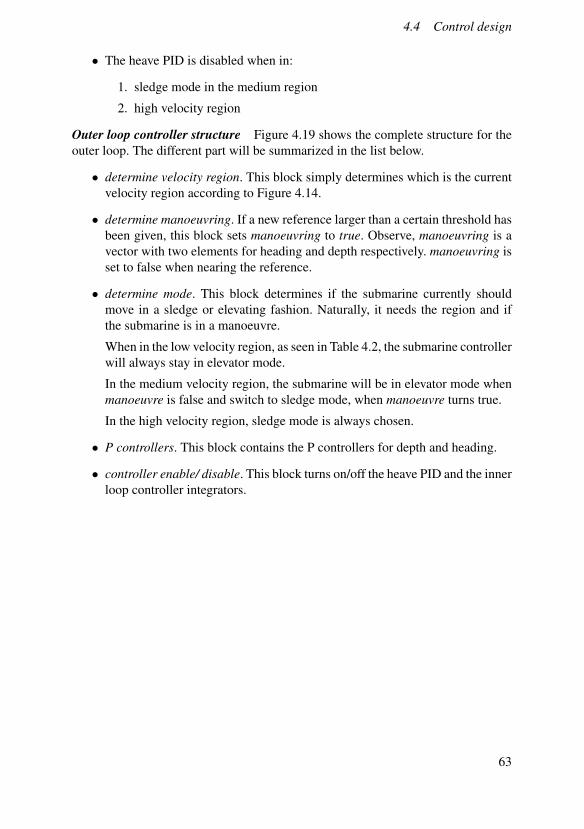
4.4 Control design

• The heave PID is disabled when in:

1. sledge mode in the medium region

2. high velocity region

Outer loop controller structure Figure 4.19 shows the complete structure for theouter loop. The different part will be summarized in the list below.

• determine velocity region. This block simply determines which is the currentvelocity region according to Figure 4.14.

• determine manoeuvring. If a new reference larger than a certain threshold hasbeen given, this block sets manoeuvring to true. Observe, manoeuvring is avector with two elements for heading and depth respectively. manoeuvring isset to false when nearing the reference.

• determine mode. This block determines if the submarine currently shouldmove in a sledge or elevating fashion. Naturally, it needs the region and ifthe submarine is in a manoeuvre.

When in the low velocity region, as seen in Table 4.2, the submarine controllerwill always stay in elevator mode.

In the medium velocity region, the submarine will be in elevator mode whenmanoeuvre is false and switch to sledge mode, when manoeuvre turns true.

In the high velocity region, sledge mode is always chosen.

• P controllers. This block contains the P controllers for depth and heading.

• controller enable/ disable. This block turns on/off the heave PID and the innerloop controller integrators.

63


Figure 4.19: Outer loop controller structure.64

5Results

5.1 Time constants and saturations

This is a collection of the time constants and submarine actuator saturations, thatwas used in the submarine simulator.

• Time constants for all the hydroplane was chosen to 3s.

• Time constant for the rotor was chosen to 6s.

• Hydroplane angle saturation was chosen to ±30◦.

• Rotor RPS was saturated to [0.6,2.4]/s to fit the velocity interval 4- 16 knots.

5.2 Final controller

Inner loop controllerState FB The state feedback gain was calculated with the weights for the differentregions as presented in Table 5.1.

State FF Table 5.2 displays the weights and conditions used to calculate the feed-forward gain Lr in the three regions, see Section 4.4 for information how this wascalculated.

region 1 2 3

Q[

500 0 00 10 00 0 10

] [100 0 00 10 00 0 10

] [100 0 00 10 00 0 10

]

R

0.1 0 0 0 0 00 0.1 0 0 0 00 0 0.1 0 0 00 0 0 0.1 0 00 0 0 0 1.0 00 0 0 0 0 1.0

0.1 0 0 0 0 00 0.1 0 0 0 00 0 0.1 0 0 00 0 0 0.1 0 00 0 0 0 1.0 00 0 0 0 0 1.0

0.1 0 0 0 0 00 0.1 0 0 0 00 0 0.1 0 0 00 0 0 0.1 0 00 0 0 0 10 00 0 0 0 0 10

Table 5.1: State FB weights.

65

Chapter 5. Results

region 1 2 3tower HPconditions

off does respondto reference in θ

off

H

1 0 0 0 0 0 0 0 0 0 0 00 1 0 0 0 0 0 0 0 0 0 00 0 1 0 0 0 0 0 0 0 0 00 0 0 1 0 0 0 0 0 0 0 00 0 0 0 − 0 0 0 0 0 0 00 0 0 0 0 − 0 0 0 0 0 00 0 0 0 0 0 1 0 0 0 0 00 0 0 0 0 0 0 1 0 0 0 00 0 0 0 0 0 0 0 1 0 0 00 0 0 0 0 0 0 0 0 1 0 00 0 0 0 0 0 0 0 0 0 50 00 0 0 0 0 0 0 0 0 0 0 50

" "

Table 5.2: State FF weights and conditions.

Integrators The numerical values will not be presented, see Section 4.4 for infor-mation about the integrators. The integrators were implemented in discrete time asmentioned in Section 2.2.

Observer The observer was also implemented in discrete time by sampling the lin-earized model. The observer gains were then calculated with white noise intensitiespresented in Equation (5.1).

E(η1 ·ηᵀ1) =

104 0 0 0 0 00 104 0 0 0 00 0 104 0 0 00 0 0 106 0 00 0 0 0 106 00 0 0 0 0 106

E(η2 ·ηᵀ2) =

10−13 0 0 0 0 0

0 10−13 0 0 0 00 0 10−11 0 0 00 0 0 10−12 0 00 0 0 0 10−12 00 0 0 0 0 10−12

(5.1)

Heave controllerAgain, the authors see no point in presenting the numerical values of the PID con-troller. As for the control error saturation, it was chosen to ±5m. The output fromthe PID saturated at ±20◦. Also the heave controller was a discrete controller.

Outer loop controllerSaturations As mentioned in Section 4.4 the P controllers for references in r andθ to the inner loop were saturated to avoid huge reference signals. The final resultsfrom these are presented in Table 5.3.

Switching To summarize, the conditions for the different outputs from the blockin Figure 4.19 are presented in Table 5.4.

66

5.3 Simulation plots

section 1 2 3r ±0.6◦/s ±1.2◦/s ±3◦/sθ ±15◦ ±15◦ ±15◦

Table 5.3: Outer loop controller saturations.


In this Section, a number of plots from different simulated manoeuvres will be pre-sented to verify that the control system works as intended. Three different test ma-noeuvres will be presented along with some of the most interesting plots.

When control efforts are plotted, they are normalized to be a percentage of themaximum control effort, i.e., fit in the interval [−1,1]. For example, the roll effortis 1 if all the rudder are saturated to maximum positive angle, see rudder orientationfor the demo submarine in Section 4.3.

Test Case OneThe first manoeuvre will be testing reference changes in heading and depth. Thistest will be performed in the middle velocity region, around 6 m/s. The first changein reference will be a change in heading, 90◦ starboard followed by 90◦ port. Afterstabilizing, a reference change in depth will be performed, starting at a depth of100m. First the submarine will dive to 120m, and then ascend to 80m. The resultsof the simulation are presented in Figures 5.1-5.4.

Heading Change As seen in Figure 5.1, a heading change of 90◦ takes approxi-mately 120 seconds in the current mode. This might not seem very fast, but as seenin Figure 5.4, the yaw effort is relatively low, which means that a faster turn is pos-sible. It can also be seen in Figure 5.3 that the submarine will pitch slightly positivewhen initiating the turn. Real submarines do also have a tendency to lower their aftswhen turning1. Figure 5.4 proves that the control system compensates for this.

Depth Change Figure 5.2 displays the depth. During the veer (0-500s), the depthalters slightly, which of course is an effect of the pitching motion. As seen in thefigure, a change of reference in depth of 20m as well as 40m takes approximately thesame time. According to Table 5.3, the pitch reference from the outer controller issaturated at ±15◦. The P part is for the current controller set to 0.3, which gives thereferences to the inner loop controller: 0.3 ·20 = 6◦, 0.3 ·40 = 12◦. Hence the pitchreference will not be saturated and the controlled system should follow somewhatlinear behaviour, i.e., double reference change = double control signal (Figure 5.4)but the same rise time.

It should also be pointed out that the depth change is in sledge mode, since thereference changes was greater than the threshold (Table 5.4). During the turn, the

1 The authors learned this fact from a co-worker at SAAB who have attended SASS product testings

67

Chapter 5. Results

regi

on1

23

regi

onac

cord

ing

toFi

gure

4.14

""

man

oeuv

ring

r ref

true

atre

fere

nce

chan

ge>

1◦,

fals

ew

hen

head

ing

erro

r<1m

and

r<

0.02

rad/

s

""

man

oeuv

ring

θre

f-

turn

sof

fata

refe

renc

ech

ange

>3.

5m,t

urns

onw

hen

dept

her

ror<

3man

dθ<

1◦tu

rns

offa

tare

fere

nce

chan

ge>

3mtu

rns

onw

hen

dept

her

ror<

3m

sled

ge/e

leva

tor

mod

eel

evat

orm

ode

sled

gem

ode

ifm

anoe

uvre

,el

seel

evat

orm

ode

sled

gem

ode

heav

ect

rlen

able

ron

!man

oeuv

reof

f

inte

grat

oren

able

forr

!man

oeuv

re&

ctrl

effo

rtr

<0.

9"

"

inte

grat

oren

able

forφ

ctrl

effo

rtφ<

0.9

""

inte

grat

oren

able

forθ

ctrl

effo

rtθ<

0.9

!man

oeuv

re&

ctrl

effo

rtθ<

0.9

!man

oeuv

re&

ctrl

effo

rtθ<

0.9

Table 5.4: Switching conditions for the outer loop controller.68


controller is in depth keeping, i.e., elevator mode, which is seen in Figure 5.4 wherethe heave controller is compensating the depth error during the turn.

Test Case TwoIn this simulation the submarine will accelerate through all three velocity regionswhile given a reference change in depth. This will show how the control systemhandles the transfer between the different controllers. The results can be seen inFigures 5.5-5.8.

Depth change A reference change is ordered at T = 100s, at the same time therotor RMS is increased and starts accelerating the submarine, see Figure 5.5. Thevelocity region changes are marked with red rings, and occurs according to Figure4.14 around 6 and 13 knots, or approximately 3.2 and 7 m/s.

Figure 5.7 displays the pitch, which in the first region is kept low. Figure 5.8shows that the bow plane heave effort is large, meaning that the submarine changesdepth in an elevating fashion, as ordered by the outer controller.

In the second region, depth changing should be performed in a sledge fash-ion (Table 4.2), meaning that it should pitch to change depth. This is confirmed inFigure 5.7, where the submarine starts to pitch after the region change. Figure 5.8shows how the aft and the tower hydroplanes work together to pitch the submarine.Worth pointing out is the acceleration of the depth change when entering the secondregion, i.e. changing from elevator mode to sledge mode. Depth changing seems tobe slower in elevator mode.

In the top speed region depth should, according to Table 4.2, only be controlledby the stern hydroplanes. This means that the control effort from the bow planesshould be zero, which can clearly be seen in Figure 5.8.

During the moments of the switches, bumps in the control efforts are distin-guishable, i.e., an effect from the gain scheduling explained in Section 4.4. This isan undesirable behaviour, but fortunately, a manoeuvre like this is probably rare.

Test Case ThreeTest case three will be similar to the previous one, except that the submarine willturn two full laps while accelerating, instead of diving. This will illustrate how theheading controller performs in the different regions. The results are shown in Fig-ures 5.9-5.12.

Heading change As in the previous test case, the changes of regions are markedwith red circles in the figures. According to Figures 5.9 and 5.10, the max speed atthe final RPS of the propeller is apparently around 7.5 m/s when turning and 9 m/swhen traveling straight.

Figure 5.11 contains an xy position graph relative to the initial position. Figure5.12 shows the control efforts and Figure 5.10, shows the heading.

69

Chapter 5. Results

As for the control effort in Figure 5.12, the controller is more aggressive in thehigh speed region than in the low and medium speed regions. This is preferred sinceoften when travelling at slow speed, the submarine should produce minimal noise.

In Figure 5.10, a noticeable increase in heading derivative takes place at thechange between the low and medium velocity region, even though the control effortis about the same. According to Section 4.3 the forces from the hydroplanes dependon the velocity u squared, it is therefore expected that the submarine will turn fasterat higher speeds.

It is worth pointing out that the roll and pitch efforts increase in magnitude as thespeed gets higher. This is noted especially for the roll effort, where it is more than50% of maximum control effort during T= 400-600s. Figure 5.13 displays zero roll.The controller is apparently compensating for huge hydrodynamic forces acting toroll the submarine. The turn is to starboard, and the roll effort says the rudders wantto roll the submarine anti-clockwise seen from behind. Thus, the forces acting onthe submarine during the turn seems to tend to roll the submarine inwards.

RotorThis is just a brief Section of how the rotor RPS translates to the submarine velocity.As seen in Figure 5.14, the relation seems to be linear, or at least affine.

70


Figure 5.1: Test case one, Heading.

Figure 5.2: Test case one, Depth.

71

Chapter 5. Results

Figure 5.3: Test case one, Pitch.

Figure 5.4: Test case one, Control Efforts.

72


Figure 5.5: Test case two, Velocity.

Figure 5.6: Test case two, Depth.

73

Chapter 5. Results

Figure 5.7: Test case two, Pitch.

Figure 5.8: Test case two, Control Efforts.

74


Figure 5.9: Test case three, Velocity.

Figure 5.10: Test case three, Heading.

75

Chapter 5. Results

Figure 5.11: Test case three, Position in the xy-plane.

Figure 5.12: Test case three, Control Efforts.

76


Figure 5.13: Test case three, roll.

Figure 5.14: RPS of the rotor vs. velocity.

77

6Discussion

6.1 Hydrodynamic Coefficients discussion

Hydrodynamic coefficients can be analytically approximated with empirical formu-las according to [Humphreys and Watkinson, 1978]. This method was applied tothe demo submarine received from FOI, and the results were compared with FOIshydrodynamic coefficients. They are both presented and compared in Table 6.1.Some coefficients differ by up to 450%, however, it can be discussed how importantaccuracy is for these coefficients.

[Humphreys and Watkinson, 1978] claims that there are 15 coefficients that aremore important than others. In Table 6.1, the error percentages between the ap-proximated and received coefficients are calculated and presented in the right mostcolumn. Some of the coefficients with the highest error percentage are not amongthe 15 most important coefficients, however, the results are still differ by large val-ues. This inaccuracy is probably the reason why this method is not commonly used,since model tests or advanced CFD calculations are much more accurate.

Table 6.1: Hydrodynamic coefficients, Measured vs. Calculated.

Coefficient FOI Measured Calculated Difference (%) Humphrey difference (%)Xu −5.8503 ·104 −3.8999 ·104 33.33 11.5Xu|u| −2.1638 ·103 −1.0567 ·104 -388.35 -Xvv 2.2024 ·104 - - -Xvr 1.9609 ·106 2.057 ·106 -4.9 8.0Xww 7.2193 ·103 - - -Xwq −1.4999 ·106 −1.8898 ·106 -26 0.1Xpr 3.7801 ·106 1.0718 ·106 71.65 -Xqq 6.0774 ·106 −3.6633 ·105 106.03 -Xrr 8.5083 ·106 1.7035 ·106 79.98 -Yv −2.1199 ·106 −2.0570 ·106 2.97 8.0Y p −3.7801 ·106 −1.0718 ·106 71.65 -Yr −1.2619 ·107 −1.7035 ·106 86.50 -Yv|v| −1.2348 ·105 - - -

78

6.1 Hydrodynamic Coefficients discussion

Yuv −1.1988 ·105 - - -Yup −1.5497 ·105 - - -Yur 1.0018 ·105 −3.8999 ·104 138.93 -Ywp 1.6215 ·106 1.8898 ·106 -16.55 0.1Ypq 1.5436 ·106 3.6633 ·105 76.27 -Zw −1.6215 ·106 −1.8898 ·106 -16.55 0.1Zq −1.5436 ·106 −3.6633 ·105 76.27 65.0Zuw −4.6835 ·104 - - -Zuq −4.8830 ·105 3.8999 ·104 107.99 -Zvp −2.1199 ·106 −2.0570 ·106 2.97 8.1Zpp - −1.0718 ·106 - -Zpr - −1.7035 ·106 - -Zww 6.5568 ·103 - - -Kv −3.7801 ·106 −1.0718 ·106 71.65 44.0K p −1.3637 ·107 −7.1006 ·106 47.93 93.0Kr −2.7968 ·107 −1.4349 ·107 48.69 -Kv|v| −8.8960 ·105 - - -Kuv −4.3689 ·105 - - -Kup −5.0448 ·106 - - -Kur −5.6544 ·106 - - -Kvw - 1.6722 ·106 - -Kvq - −2.0698 ·106 - -Kwp 3.7801 ·106 1.0719 ·106 71.64 -Kwr - 2.0698 ·106 - -Kqr −7.5 ·107 −3.33 ·107 55.6 -Mw −4.2177 ·106 −3.6633 ·105 91.31 64.0Mq −3.9850 ·108 −3.6229 ·108 9.09 10.0Mw|w| -4.4401·105 - - -Muw 5.4147 ·105 5.5523 ·105 -2.54 -Muq −2.3875 ·107 1.8898 ·106 107.92 -Mvp - 1.7035 ·106 - -Mvr - −1.0718 ·106 - -Mpp - 1.4349 ·107 - -Mpr 4.5986 ·108 3.8849 ·108 15.52 11.4Mrr - 1.4349 ·107 - -Nv 4.8619 ·105 −1.7035 ·106 450.38 -N p −2.7968 ·107 −1.4349 ·107 48.69 -Nr −4.7351 ·108 −3.9559 ·108 16.46 10.7Nv|v| 9.7812 ·105 - - -Nuv −2.2747 ·106 −2.0180 ·106 11.29 -Nup −1.6776 ·106 −1.0718 ·106 36.11 -Nur −3.4493 ·107 −1.7035 ·106 95.06 -Nvq - 1.0718 ·106 - -Nwp - −3.6633 ·105 - -Npq −3.8486 ·108 −3.5519 ·108 7.71 10.7

79

Chapter 6. Discussion

Nqr - 1.4349 ·107 - -

6.2 Linearised state space model

A total of three linear state space system were derived in this thesis. A short discus-sion of the third model, i.e., the high velocity region, is presented here. The modelitself is presented in Figure 6.1. Some parts of the state space system is what canbe expected. The hydroplanes follow a first order characteristics with time constantT = 3. The system was linearised with no roll/pitch, hence φ and θ are the integralsof p and q. As for the u characteristics, rudder angles δ1, δ2, δ5 and δ6 give a pos-itive addition to u. This appear as strange at a first glance, and the Coriolis effectfrom the six degrees of freedom dynamics is most likely the source of this.

How rudder angles influence the acceleration, e.g., r, differs between the rud-ders. This does also seem strange and is most likely also caused by the Corioliseffect.

6.3 Controller issues

The control system contains numerous numbers of nonlinearities in forms of satu-rations and logical switches, especially in the outer loop. Nonlinearities in the loopcan be a source of possible oscillations. These can be difficult to locate, but in thissection a few possible origins for oscillations and other controller problems will bediscussed.

Sledge mode depth controlDepth control in sledge mode is performed by a P controller in cascade with an innerloop state feedback/feedforward controller with an integrated I part. The I part isdisabled at the moment of a reference change and reenabled when the control erroris less than 3m and the pitch is less then 1◦, see Table 5.4. The reason to includean I part is to remove stationary errors, but a stationary error greater than 3 metersfrom the reference point will not enable the I part, hence, continue to exist.

Since the pitch has to be less then 1◦ to enable the I part, this could be a sourceof oscillations around a reference depth.

These effects have at this point not yet shown up. Either do they not exist at all,or perhaps only appear at special cases. Introducing disturbances could perhaps alsomake these effects show up.

Course controlAnalogous with the sledge depth control, the course control could experience thesame problems, although, has not at this point.

80

6.3 Controller issues

Figure 6.1: Linear model in the high velocity region.

81


Overly complicated controllerThe final control structure can feel a bit overambitious. The controller could havebeen simplified by adding PID controllers in the r,φ and θ directions. This wouldremove the state FF, FB and the observer part and turn the I parts controller intoPIDs. Hopefully, however, this would result in a poorer performing controller butwith increased simplification.

An LQ controller relies on the state space model to be relatively accurate. If thecontroller presented in this thesis would be implemented in a real submarine andturn out to be inadequate, tuning it, is not straightforward since it requires tuningof the model itself. A PID however, is simpler to tune on spot. The PIDs in thesubmarine could, e.g., be based on a PID design derived in the lab, and then tunedby changing the P, I, and D gains1.

6.4 Future Work

This master thesis is only the start of a project that could be developed much further.This means that there are lots of room for future work and improvements.

ModelSensor Models Measured values from sensors always come with an uncertainty.Adding noise to measured signals in the submarine simulator, is a step closer to testhow the controller will perform in an actual vessel.

On a submarine, some sensor errors will differ depending on where the sensoris placed. For example, the velocity sensor is often a pressure sensor placed on thesubmarine hull. If the flow around the hull is turbulent, this could cause large noiselevels to the log.

The water pressure due to the suppressed water by the submarine bow can alsochange over the hull. Multiple pressure sensors placed at different locations aretherefor often used. The measured log velocity is then a function of measured valuesfrom each sensor.

In Section 3.1, the added mass effect was explained, i.e., the water closest to thehull travels with the submarine, hence, increasing the apparent mass. This could beanother source of a velocity log sensor inaccuracy. The sensor could measure thesubmarine’s velocity relative the water closest to the hull, which is lower then thevelocity relative the unaffected water, further away from the hull.

Currently, the measured depth is the depth of the submarine-fixed frame’s origin.It can be discussed if this is the actual depth of the submarine. Perhaps the subma-rine’s depth is the part of the submarine, that is deepest, which could be preferredwhen manoeuvring close to the seabed.

1 There are more complex PID designs than the one presented in this thesis. A more complex PIDdesign could include additional tuning parameters.

82

6.4 Future Work

Tank System A submarine includes a number of different tanks which are used tocontrol whether to sink or float, as well as the attitude of the submarine. Adding thetanks as possible actuators is a step closer to a perfect submarine simulator.

A simple way to model the effects from the tanks, is the possibility to affect theposition of the center of gravity, and the weight of the submarine. A more accuratemodel of the tank system, could be to model the pump dynamics as well as the flowcharacteristics in the tanks and tubes.

Additional Hydrodynamic Effects There are more hydrodynamic effects thatneed to be taken into account for a complete simulator system. Among them aredifferent effects that occur near the surface or near the bottom.

At the moment, it is only possible to specify a linear current in a specific di-rection in the simulation. It might be useful, to also be able to simulate irregularcurrents and turbulence, to see how the controller handles these conditions, since itis closer to the reality.

Simulating Alarms An important duty of the SASS, is error detection and alarmpresentation. This indicates to the helmsman if anything has malfunctioned on thesubmarine, for example a hydroplane angle fault or pump malfunction. It wouldtherefore be useful to be able to simulate these alarms, and present them to the userof the simulator system. These errors should also be sent to the autopilot, if, forexample, a hydroplane is not responding, the autopilot should take this into accountwhen steering the submarine.

ImplementationThe focus of the thesis have been mostly on physical modelling and controller de-sign, and less on the program for target system, i.e., the test rig. This means thatthere is a lot of room for improvement here, especially within usability.

User Interface The test rig has a software version of a hardware console in asubmarine. The original goal was to implement the simulator system with the in-terface, but due to the unexpected complexity of hydrodynamic modelling, this waspostponed as a future project.

At the moment, the simulator system is communicated with through the terminalin Linux. A sensor value or a new reference, has to be explicitly requested by aterminal command. This is not a user friendly setup, which is the reason why thesimulator system needs to be implemented with the test rig user interface in orderto properly benefit from the submarine simulator.

In a far future, it might also be desirable to implement compatibility with exist-ing hardware from a submarine, to be able to train personnel on land.

Animation A simple animation of the submarine attitude and hydroplane positionwas developed in Simulink. A picture of the animations can be found in Figure 6.2.At the moment, the animations are only available when simulating the submarine inSimulink, and not when running the simulator on the target system, hence, a desired

83


Figure 6.2: Rudder and submarine attitude animation.

feature could be to implement a TCP communication with the animations and thesubmarine simulator.

84

Bibliography

ActiveState. Tool command language. URL: http://www.tcl.tk/ (visited on07/08/2014).

Åström, K. J. and C. G. Källström (1976). Identification of ship steering Dynamics.Tech. rep.

Feldman (1979). DTNSRDC Revised standard submarine equations of motion.Tech. rep. Carderock Division of the Naval Surface Warfare Center, Maryland,USA.

Fossen, T. (2011). Marine Craft Hydrodynamics and Motion Control. John WileySons Ltd.

Fossen, T. I. (1994). Guidance and Control of Ocean Vehicles. John Wiley SonsLtd.

Fossen, T. I. and O.-E. Fjellstad (1995). Nonlinear Modeling of Marine Vehiclesin 6 Degrees of Freedom. Tech. rep. The Norwegian Institude of Technology,Trondheim, Norway.

Glad, T. and L. Ljung (2003). Reglerteori. Studentlitteratur AB Lund.Hickey, R. I. (1990). Submarine motion simulation including zero forward speed

and propeller race effects. Tech. rep. MIT, Department of Ocean Engineering,Massachusetts, USA.

Humphreys and Watkinson (1978). Prediction of acceleration hydrodynamic coef-ficients for underwater vehicles from geometric parameters. Tech. rep. NavalCoastal System Laboratory, Florida, USA.

Lamb, S. H. (1932). Hydrodynamics. University Press, New York, USA.Larsson, L. and H. Raven (2010). Ship resistance and flow. The society of Naval

Architects and Marine Engineers.Mathworks. Matlab. URL: http://www.mathworks.se/products/matlab/

(visited on 07/08/2014).Mathworks. Simulink. URL: http://www.mathworks.se/products/simulink/

(visited on 07/08/2014).

85

Bibliography

Ridley, P., J. Fontan, and P. Corke (2003). Submarine Dynamic Modeling. Tech. rep.Queensland University of Technology, Queensland, Australia.

Toxopeus (2011). Practical application of viscous-flow calculations for the simu-lation of manoeuvring ships. PhD thesis. Maritime Reasearch Institute Nether-lands.

Watt (2007). Modelling and Simulating Unsteady Six Degrees-of-Freedom Subma-rine Rising Maneuvers. Tech. rep. Defence Research and Development Canada,Atlantic, Canada.

86

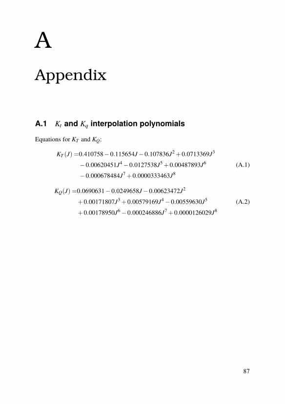
AAppendix

A.1 Kt and Kq interpolation polynomials

Equations for KT and KQ:

KT (J) =0.410758−0.115654J−0.107836J2 +0.0713369J3

−0.00620451J4−0.0127538J5 +0.00487893J6

−0.000678484J7 +0.0000333463J8

(A.1)

KQ(J) =0.0690631−0.0249658J−0.00623472J2

+0.00171807J3 +0.00579169J4−0.00559630J5

+0.00178950J6−0.000246886J7 +0.0000126029J8

(A.2)

87

Lund UniversityDepartment of Automatic ControlBox 118SE-221 00 Lund Sweden

Document nameMASTER´S THESISDate of issueSeptember 2014Document NumberISRN LUTFD2/TFRT--5954--SE

Author(s)

Erik LindMagnus Meijer

SupervisorHans Bohlin, SaabKarl-Erik Årzén, Dept. of Automatic Control, Lund University, Sweden (examiner)Sponsoring organization

Title and subtitle

Simulation and Control of Submarines

Abstract

When designing control systems for real applications, it is important to first do testing in a simulated environment, to ensure adequate performance. This is especially important when designing control systems for applications that have high operation costs, e.g., submarines, since late errors in the development can be extremely costly.Saab develops steering systems for submarines. Prior to this thesis, testing for those have been

performed in an open-loop environment, where only static test cases could be examined. Saab therefore identified the need to implement a dynamic test simulator, which could react to the different signals from the steering system, i.e., act as a real submarine.In this thesis, such a simulator was developed. It consists of two parts, a physical model of a

submarine, and a control system for motion control. As for the physical submarine model, it can be approximated from mechanical data of a submarine that the user provide, such as dimensions and weight. The second options is for the user to explicitly supply the simulator with hydrodynamic coefficients.The control system was derived to control a model of a demo submarine. Saab is also involved in

submarine navigation systems and saw the need to, in the future, also have the possibility to test those products. A navigation system assumes an autopilot exists, hence, an autopilot control system was developed.In the end, the control system consisted of a two-level cascade controller of mixed LQG- and PID-

control, along with a Kalman estimator for estimating unknown states.The results were overall satisfactory. The performance of the control system is well within usual

customer specifications and the main problems in this thesis lay in getting a proper model.

Keywords

Classification system and/or index terms (if any)

Supplementary bibliographical information

ISSN and key title0280-5316

ISBN

LanguageEnglish

Number of pages1-87

Recipient’s notes

Security classification

http://www.control.lth.se/publications/

Simulation and Control of Submarines - Lunds...

Documents

Transcript of Simulation and Control of Submarines - Lunds...