Simulation and Control of Guided Ram Air Parafoils · PDF file29.08.2006 ·...

Simulation and Control ofGuided Ram Air Parafoils

by

Brent Edward Tweddle

A reportpresented to the University of Waterloo

in fulfilment of therequirement for the course of

ECE 499in the

Department of Electrical and Computer Engineering

Waterloo, Ontario, Canada, 2006c© Brent Tweddle, 2006

August 2006

I hereby confirm that I have received no further help other than what is men-tioned in writing this report. I also confirm this report has not been previouslysubmitted for academic credit at this or any other academic institution.

———————Brent Edward Tweddle20107755August 29, 2006

ii

Abstract

This report describes the investigation of the modeling, simulation and controlof a guided ram air parafoil. The purpose of this research is to develop a systemthat can deliver a payload through a one meter by one meter window. Althoughthis goal was not achieved, this investigation represents the fist stage of researchtoward this goal. This report presents the basics of parachute flight, the detailsof the modeling and simulation for a six degree of freedom system and the designof the guidance and control system. Conclusions and future recommendations arepresented at the end of this report.

iii

Acknowledgments

There are a number of people that I would like to thank for their help in prepar-ing and writing this report.

I am grateful to my supervisor Professor David Wang for all of the assistanceand support he has provided in all stages of writing this report. I would like tothank Matthew Black for his help with the parachute and for answering my manyquestions on mechanics and dynamics. Rick Hummel and the rest of the staff atthe Waterloo Region Emergency Services Training and Research Center have beenvery helpful in providing such an excellent testing location for the parachute freeof charge.

iv

Contents

1 Introduction 1

2 Overview of Parachute Design 4

2.1 Parafoil Deployment . . . . . . . . . . . . . . . . . . . . . . . . . . 7

2.2 Parafoil Design Parameters . . . . . . . . . . . . . . . . . . . . . . . 9

3 Overview of Dynamic Models 12

4 Six Degree-of-Freedom Modelling and Simulation 14

4.1 Derivation of Rigid Body Equations . . . . . . . . . . . . . . . . . . 15

4.1.1 Force Equations . . . . . . . . . . . . . . . . . . . . . . . . . 18

4.1.2 Moment Equations . . . . . . . . . . . . . . . . . . . . . . . 18

4.1.3 Navigation Equations . . . . . . . . . . . . . . . . . . . . . . 19

4.1.4 Kinematic Equations . . . . . . . . . . . . . . . . . . . . . . 19

4.1.5 Summary of Rigid Body Equations . . . . . . . . . . . . . . 20

4.2 Generation of Forces and Moments . . . . . . . . . . . . . . . . . . 21

4.2.1 Free Body Diagram . . . . . . . . . . . . . . . . . . . . . . . 21

4.3 Apparent Mass Effects . . . . . . . . . . . . . . . . . . . . . . . . . 26

4.4 Wind Disturbances . . . . . . . . . . . . . . . . . . . . . . . . . . . 30

4.5 Sensor Dynamics . . . . . . . . . . . . . . . . . . . . . . . . . . . . 31

4.6 Parachute System Parameters . . . . . . . . . . . . . . . . . . . . . 32

4.7 Simulation Results . . . . . . . . . . . . . . . . . . . . . . . . . . . 34

v

5 Nine Degree of Freedom Simulation 41

6 Guidance, Navigation and Control System Design 43

6.1 Guidance System . . . . . . . . . . . . . . . . . . . . . . . . . . . . 45

6.2 Navigation . . . . . . . . . . . . . . . . . . . . . . . . . . . . . . . . 47

6.3 Linearization . . . . . . . . . . . . . . . . . . . . . . . . . . . . . . 49

6.4 System Identification . . . . . . . . . . . . . . . . . . . . . . . . . . 59

6.5 Control . . . . . . . . . . . . . . . . . . . . . . . . . . . . . . . . . 61

6.5.1 Pole Placement . . . . . . . . . . . . . . . . . . . . . . . . . 61

6.5.2 H-Infinity Control . . . . . . . . . . . . . . . . . . . . . . . . 63

6.5.3 Model Predictive Control . . . . . . . . . . . . . . . . . . . . 64

7 Conclusions and Future Recommendations 65

7.1 Conclusions . . . . . . . . . . . . . . . . . . . . . . . . . . . . . . . 65

7.2 Future Recommendations . . . . . . . . . . . . . . . . . . . . . . . 66

A Fourth Order Runge-Kutta Method 67

B Matlab m-Files 69

vi

List of Figures

1.1 WARG Guided Ram Air Parachute . . . . . . . . . . . . . . . . . . 3

2.1 United States Marine Corps MC1-1C[31] . . . . . . . . . . . . . . . 5

2.2 Drawings from Original Parafoil Patent[25] . . . . . . . . . . . . . . 6

2.3 Simplified Illustration of Ram Air Parafoil and Payload[19] . . . . . 7

2.4 Parafoil Canopy[28] . . . . . . . . . . . . . . . . . . . . . . . . . . . 8

2.5 Display Jumper Landing a Ram Air Parachute[43] . . . . . . . . . . 9

2.6 Parafoil Angles[29] . . . . . . . . . . . . . . . . . . . . . . . . . . . 10

2.7 Dihedral and Anhedral Angles[29] . . . . . . . . . . . . . . . . . . . 11

3.1 NASA X-38 Parachute System [1] . . . . . . . . . . . . . . . . . . . 13

4.1 Roll, Pitch and Yaw Directions for an Airplane [38] . . . . . . . . . 15

4.2 Longitudinal Free Body Diagram of Ram-Air Parachute System[29] 21

4.3 Ram Air Parafoil Coefficient of Lift for Various Aspect Ratios[29] . 23

4.4 Longitudinal Aerodynamic Coefficients[22] . . . . . . . . . . . . . . 23

4.5 Lateral Aerodynamic Database for 10o Rigging Angle[29] . . . . . . 24

4.6 Lateral Aerodynamic Database for 13o Rigging Angle[29] . . . . . . 24

4.7 Parafoil Geometry[30] . . . . . . . . . . . . . . . . . . . . . . . . . 29

4.8 Volumetric Representations of Apparent Mass and Moments[30] . . 29

4.9 No Control Input . . . . . . . . . . . . . . . . . . . . . . . . . . . . 34

4.10 No Control Input: XYZ Position - North, East, Up (m) . . . . . . . 35

4.11 No Control Input: XYZ Velocity - Body Fixed Axis (m/s) . . . . . 36

vii

4.12 No Control Input: Euler Angles (degrees) . . . . . . . . . . . . . . . 36

4.13 No Control Input: Angular Rates (degrees per second . . . . . . . . 37

4.14 No Control Input: Angle of Attack (degrees) . . . . . . . . . . . . . 37

4.15 No Control Input: Net Velocity (m/s) . . . . . . . . . . . . . . . . . 38

4.16 Braking Control Input . . . . . . . . . . . . . . . . . . . . . . . . . 38

4.17 Braking Control Input: XYZ Position - North, East, Up (m) . . . . 39

4.18 Braking Control Input: XYZ Velocity - Body Fixed Axis (m/s) . . 39

4.19 Braking Control Input: Euler Angles (degrees) . . . . . . . . . . . . 40

6.1 Guidance, Navigation and Control System . . . . . . . . . . . . . . 43

6.2 Pole Placement with Integral Control Block Diagram . . . . . . . . 61

viii

List of Tables

4.1 Simulator Parameter Values . . . . . . . . . . . . . . . . . . . . . . 32

4.2 Aerodynamic Coefficient Values . . . . . . . . . . . . . . . . . . . . 33

ix

Chapter 1

Introduction

The University of Waterloo Aerial Robotics Group (WARG) is competing in theInternational Aerial Robotics Competition (IARC) that requires teams to builda system of autonomous aerial vehicles that can complete a specific mission thatconsists of a number of stages must be completed. The first stage requires theteam to fly a vehicle through a three kilometer course of Global Positioning System(GPS) way-points to a final destination. In the second stage, the team’s vehiclesmust search the area for a building with a specific visual symbol, and find a onemeter by one meter open window on that building. The requirements of the thirdstage are to enter the open window and search the interior of the building forvisual reconnaissance information. The fourth and final stage requires the team tocomplete the first three levels together in less than 15 minutes [33].

The IARC does not specify what types of vehicles can be used to accomplishthese objectives. WARG has chosen a unique strategy that utilizes a system ofmultiple vehicles together as a coordinated system. A fixed wing aircraft will flythe three kilometer course and search the city with onboard cameras. Once theairplane has found the open window it will launch a small guided ram air parafoilthat will enter the window and deliver a small ground robot. The small groundrobot will drive through the interior of the building searching for the necessaryinformation [11].

A fixed wing aircraft was chosen to travel the distance and search the citybecause it is a naturally stable platform and it can travel at high speeds. Otheruniversity teams have chosen a helicopter [15, 10] for this role for its hoveringcapabilities, however a helicopter is naturally unstable [14]. Additionally, a smallhelicopter can not travel as fast as an airplane. The last stage of the mission will be

1

performed by a small ground robot that is simple, light weight and maneuverable[11].

A number of options exist for how to get a small vehicle through the window andinside the building. Teams that are using helicopters plan to lower the helicopterto the same altitude as the window and then either extend an arm through thewindow that drops off their robot, or shoot their robot into the building with asmall compressed gas canon. WARG feels that there is a very high likelihoodthat the helicopter blades may make contact with a nearby object resulting in acatastrophic crash [11]. Other teams that are using airplanes like WARG, haveconsidered launching ballistic missiles through the window with minimal levels ofcontrol [27]. This drawback of this strategy is that there exists the risk that thevehicle will enter the window with a very high speed, which means there is verylittle chance for trajectory correction and the system may be damaged on impact.

For this reason, WARG proposed the use of a small ram air parachute [11] toenter the window as seen in Figure 1.1. Ram air parachutes are naturally stable,highly maneuverable and fly at a relatively slow speed. A ram air parachute wouldbe dropped from an airplane at an altitude of 200 to 700 feet above ground level.An onboard computer would be given the co-ordinates of the target window andwould guide the parachute through the window using measurements from a GPSand attitude heading reference system (AHRS).

This poses a very difficult problem for the parachute. It must be able to hita one meter by one meter window on the side of a building while correcting forany wind disturbances caused by flying in an urban area. Other errors will bepresent in the co-ordinates in the window due to the fact that these co-ordinateswere measured from a camera onboard a moving airplane.

Although this goal may seem very difficult, skilled skydivers can consistentlyjump from 1000 feet and hit their target within three centimeters [6]. Additionally,commercial autonomous parachutes in industry are now able to land within 75meters of their target when dropped from 25,000 feet [24]. As a result, it is believedthat this goal is difficult, but not impossible.

The ability to control a ram air parafoil is a topic that has been investigatedfrom a number of perspectives in various published papers. Slegers and Costello [39],[40] derive a dynamic model for a small guided parachute and present a method forcontrolling it using model predictive control. Their experimental results allow themto land within six feet of their desired target. Jann [26] discussed a simplified threeand four degree of freedom model for a parafoil along with the design of a guidance,navigation and control system that was successfully simulated to include sensor

2

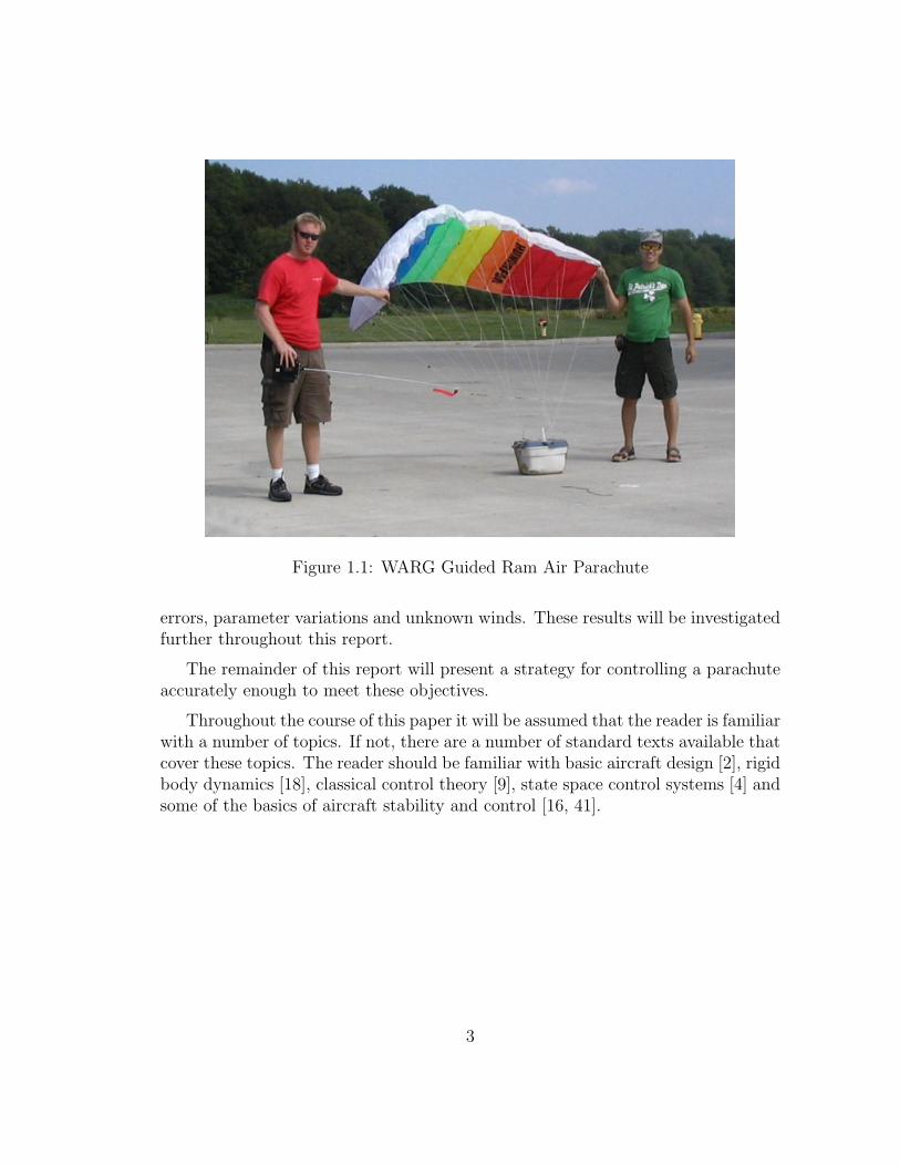
Figure 1.1: WARG Guided Ram Air Parachute

errors, parameter variations and unknown winds. These results will be investigatedfurther throughout this report.

The remainder of this report will present a strategy for controlling a parachuteaccurately enough to meet these objectives.

Throughout the course of this paper it will be assumed that the reader is familiarwith a number of topics. If not, there are a number of standard texts available thatcover these topics. The reader should be familiar with basic aircraft design [2], rigidbody dynamics [18], classical control theory [9], state space control systems [4] andsome of the basics of aircraft stability and control [16, 41].

3

Chapter 2

Overview of Parachute Design

Parachute systems are used for a large variety of applications ranging from pay-load delivery to braking applications. All of these types of systems are technicallyreferred to by the term aerodynamic decelerators. This report focuses on the ap-plication of a parachute system for payload delivery.

The basic design for a payload delivery system has two main components, aheavy payload that is connected by a set of lines to a light weight fabric parachute.There are a large variety of designs for the parachute and payload components. Thepayload design is normally constrained by the application; however the payload isnormally designed to have structural integrity, reduce aerodynamic drag, supportparachute inflation. In some cases the payload includes a propulsion system to addthrust to the system. In this report, payload design will not be investigated and itwill be assumed that no propulsion system is used.

The simplest parachute design is the circular ballistic parachute. This canopyappears hemispherical in design when fully inflated and decreases the speed of thepayload by increasing drag. Parachutes of this type can not glide long distancesand are not maneuverable. The basic circular parachute design was modified touse vents on either side of the canopy to allow maneuverability. Opening a vent onone side of the parachute would cause air to escape on that side and create a netthrust in the opposite direction. The most popular parachute of this type was theMC1-1B military personnel parachute[28] shown below in Figure 2.1.

More complex canopy designs offer better performance than the circular parachute.The most popular example is the ram air parafoil that was patented in 1966 byJalbert[25]. The drawings from this patent can be seen in Figure 2.2. A simplifiedillustration of this system can be seen in Figure 2.3.

4

Figure 2.1: United States Marine Corps MC1-1C[31]

The main benefit of this design is that it offers the highest glide ratio (Lift/Dragratio). The ram air parafoil glide ratio generally ranges from 2.8 to 3.5 while theglide ratio of the MC1-1B is only 0.75 [28]. The remainder of this report will focusonly on ram air parafoils. Other types of canopy designs for parachute systems aredescribed by Knacke [28].

Figure 2.4 shows a side profile of the ram air parachute along with a top viewdiagram of the rectangular parafoil design. The ram air parachute has the crosssection of an airfoil and is essentially an inflatable wing. Typically an airfoil with agood lift to drag ratio is chosen to maximize the gliding performance. The Clark Yairfoil is a popular airfoil choice. Although recently airfoils from gliders have beenused such as the Lissaman 7808 [29]. The top-down shape of the canopy, calledthe planform, is usually rectangular or elliptical with a low aspect ratio. Ellipticalparafoils are similar to rectangular parafoils, except that in order to offer higher

5

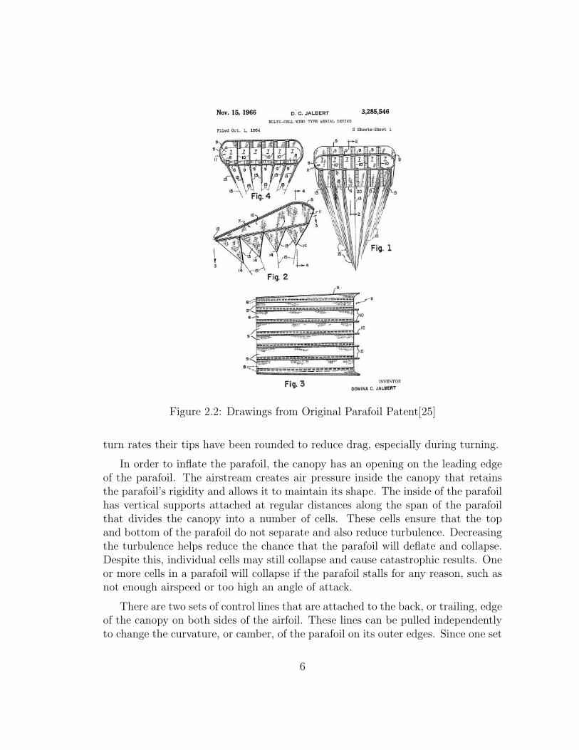
Figure 2.2: Drawings from Original Parafoil Patent[25]

turn rates their tips have been rounded to reduce drag, especially during turning.

In order to inflate the parafoil, the canopy has an opening on the leading edgeof the parafoil. The airstream creates air pressure inside the canopy that retainsthe parafoil’s rigidity and allows it to maintain its shape. The inside of the parafoilhas vertical supports attached at regular distances along the span of the parafoilthat divides the canopy into a number of cells. These cells ensure that the topand bottom of the parafoil do not separate and also reduce turbulence. Decreasingthe turbulence helps reduce the chance that the parafoil will deflate and collapse.Despite this, individual cells may still collapse and cause catastrophic results. Oneor more cells in a parafoil will collapse if the parafoil stalls for any reason, such asnot enough airspeed or too high an angle of attack.

There are two sets of control lines that are attached to the back, or trailing, edgeof the canopy on both sides of the airfoil. These lines can be pulled independentlyto change the curvature, or camber, of the parafoil on its outer edges. Since one set

6

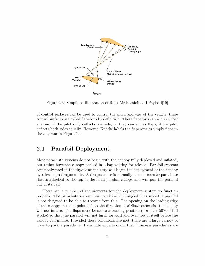
Figure 2.3: Simplified Illustration of Ram Air Parafoil and Payload[19]

of control surfaces can be used to control the pitch and yaw of the vehicle, thesecontrol surfaces are called flaperons by definition. These flaperons can act as eitherailerons, if the pilot only deflects one side, or they can act as flaps, if the pilotdeflects both sides equally. However, Knacke labels the flaperons as simply flaps inthe diagram in Figure 2.4.

2.1 Parafoil Deployment

Most parachute systems do not begin with the canopy fully deployed and inflated,but rather have the canopy packed in a bag waiting for release. Parafoil systemscommonly used in the skydiving industry will begin the deployment of the canopyby releasing a drogue chute. A drogue chute is normally a small circular parachutethat is attached to the top of the main parafoil canopy and will pull the parafoilout of its bag.

There are a number of requirements for the deployment system to functionproperly. The parachute system must not have any tangled lines since the parafoilis not designed to be able to recover from this. The opening on the leading edgeof the canopy must be pointed into the direction of airflow; otherwise the canopywill not inflate. The flaps must be set to a braking position (normally 50% of fullstroke) so that the parafoil will not lurch forward and over top of itself before thecanopy can inflate. Provided these conditions are met, there are a large variety ofways to pack a parachute. Parachute experts claim that ”‘ram-air parachutes are

7

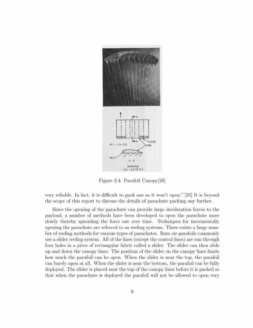
Figure 2.4: Parafoil Canopy[28]

very reliable. In fact, it is difficult to pack one so it won’t open.”’[35] It is beyondthe scope of this report to discuss the details of parachute packing any further.

Since the opening of the parachute can provide large deceleration forces to thepayload, a number of methods have been developed to open the parachute moreslowly thereby spreading the force out over time. Techniques for incrementallyopening the parachute are referred to as reefing systems. There exists a large num-ber of reefing methods for various types of parachutes. Ram air parafoils commonlyuse a slider reefing system. All of the lines (except the control lines) are run throughfour holes in a piece of rectangular fabric called a slider. The slider can then slideup and down the canopy lines. The position of the slider on the canopy lines limitshow much the parafoil can be open. When the slider is near the top, the parafoilcan barely open at all. When the slider is near the bottom, the parafoil can be fullydeployed. The slider is placed near the top of the canopy lines before it is packed sothat when the parachute is deployed the parafoil will not be allowed to open very

8

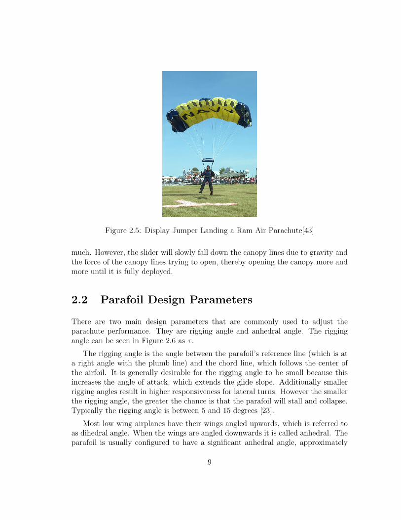
Figure 2.5: Display Jumper Landing a Ram Air Parachute[43]

much. However, the slider will slowly fall down the canopy lines due to gravity andthe force of the canopy lines trying to open, thereby opening the canopy more andmore until it is fully deployed.

2.2 Parafoil Design Parameters

There are two main design parameters that are commonly used to adjust theparachute performance. They are rigging angle and anhedral angle. The riggingangle can be seen in Figure 2.6 as τ .

The rigging angle is the angle between the parafoil’s reference line (which is ata right angle with the plumb line) and the chord line, which follows the center ofthe airfoil. It is generally desirable for the rigging angle to be small because thisincreases the angle of attack, which extends the glide slope. Additionally smallerrigging angles result in higher responsiveness for lateral turns. However the smallerthe rigging angle, the greater the chance is that the parafoil will stall and collapse.Typically the rigging angle is between 5 and 15 degrees [23].

Most low wing airplanes have their wings angled upwards, which is referred toas dihedral angle. When the wings are angled downwards it is called anhedral. Theparafoil is usually configured to have a significant anhedral angle, approximately

9

Figure 2.6: Parafoil Angles[29]

20 degrees, which is commonly referred to as crown rigging. Both dihedral andanhedral angles are illustrated in Figure 2.7 as β. This is also different from flatrigging, which has a very small anhedral angle and is sometimes used in parachutesthat are designed to be sluggish for beginning skydivers.

The turning method for a parafoil differs from that of a normal airplane. Anairplane will use its differential control surfaces to roll the vehicle and use its lift toturn in the direction of the bank. A parafoil will use its flaperons in a differentialmode to increase the differential drag across the span of the parafoil. This causesthe vehicle to skid through a turn without banking. It is important to note that aparafoil would turn in the opposite direction that an airplane would turn with thesame aileron deflections. In other words, if the starboard surface was set down andthe port surface set up on an airplane and a parafoil, the airplane would turn inthe port direction while the parafoil would turn in the starboard direction. Despitethe fact that a parafoil uses skid turning it will still enter a bank due to centrifugalforces acting on the payload. This bank will be very large since the payload body

10

Figure 2.7: Dihedral and Anhedral Angles[29]

is far below the parafoil.

The crown rigging is largely responsible for the skid turning in parafoils. Thisis because the deflection on the edges of the parafoil creates an increase in lift thatdoes not contribute much towards a banking moment because it is angled outwardsbecause of the anhedral angle. However the drag is not affected by the anhedralangle and continues to produce differential drag that contributes towards the skidturning moment. Therefore an increase in the anhedral angle causes faster turningperformance. However the tradeoff is that there is less lift, which reduces the glideratio[23].

11

Chapter 3

Overview of Dynamic Models

The dynamic models for ram air parachutes can generally be broken down into twocategories; those that model the parachute and payload as a single rigid body orthose that model them as two seperate bodies. As a single rigid body the parafoilis assumed to be lock in position and orientation with the payload. In the twobody models, there are a number of degrees of freedom between the parafoil andpayload. In these systems the number of degrees of freedom can range from onlyone or two degrees of freedom (for example if the payload can only rotate on theyaw axis with respect to the parafoil) to a full six degrees of freedom where allaspects of the payload can move with respect to the parafoil.

A number of papers describe the single rigid body approach using six degrees offreedom [39], [37], [13]. The models that utilize two seperate rigid bodies usuallyassume the positions of the two bodies are fixed with respect to each other and thatonly the attitude of the two bodies will be different. This results in dynamic modelsthat have eight [22], [21] and nine [40] degrees of freedom [40]. It is interesting tonote that three and four degree of freedom models were developed by Jann [26],however they are only claimed to be valid in steady state conditions.

It is worthwhile to note that the only experimental work that was done usingthe two body approach [22, 21] used a parafoil that had a 121.5 feet span and canbe seen in Figure 3.1.

It is reasonable to assume that a small parachute system will experience smallerdifferences in attitude between the payload and parafoil that a large parachutesystem will. This seems intuitive because the wind disturbances in the area will bemore different the further away two objects are.

All dynamic models will build up the forces and moments on the parafoil by

12

Figure 3.1: NASA X-38 Parachute System [1]

utilizing aerodynamic stability derivatives that may be linear or non-linear. Theexperimental identification and derivation of these coefficients are the topic of anumber of papers [39], [40], [37], [22], [21], [13] and [5]. This type of model considersuncertainty as variation in the aerodynamic coefficients and disturbances, such aswind, as additive forces and moments.

13

Chapter 4

Six Degree-of-Freedom Modellingand Simulation

In the chapter a six degree of freedom model will be used to simulate a ram airparachute system. This model uses three degrees of freedom for position and threedegrees of freedom for orientation. The orientation uses Euler angles which con-tain singularities at certain orientations. This problem could be avoided by usingquaternions, which create a seven degree of freedom model; however since it canbe assumed that the parachute vehicle will fly mostly straight and level, the use ofEuler angles is acceptable for this application.

The six degree of freedom model assumes that the payload will remain at afixed orientation and location with respect to the parafoil. This can be a validassumption for parachute systems where the payload and parafoil are close enoughto each other that they both experience the same wind effects. This assumptioncan be invalidated by high gusting winds, parafoil collapse or extreme maneuvers.Models with more than six degrees of freedom will be briefly discussed later in thisreport.

The following sections will outline the development of a six degree of freedomsimulator that was implemented in Matlab[32].

14

4.1 Derivation of Rigid Body Equations

Six degree of freedom equations of motion are presented by Stevens and Lewis andderived throughout the course of their text[41]. They assume that the earth can bemodelled as a flat plane and that the rotation of the earth is negligable, which isvalid for short flights covering small areas. In this section, these equations will bepresented and derived in a form that is directly applicable building a state spacemodel for a parachute system.

To begin, let φ, θ and ψ represent the roll, pitch and yaw of the vehicle respec-tively and let P , Q and R represent the roll, pitch and yaw rates respectively. Theroll, pitch and yaw directions are shown in Figure 4.1. Also, let pN , pE and pU rep-resent the location of the rigid body in the inertial reference frame using the north,east and up convention. Let U , V and W represent the velocity of the vehicle withrespect to the body fixed axes. It is important to note that it is convention in theaerospace industry to use the velocity of the vehicle with respect to the body framerather than the inertial frame. This convention is not used in other industries,however it makes sense in aerospace applications since these are the velocities thata pilot onboard the vehicle would see. From the pilot’s perspective in an aircraft,the U velocity is positive in the forward direction towards the nose of the plane.The V velocity is positive in the starboard direction and the W velocity is positivein the downwards direction.

Figure 4.1: Roll, Pitch and Yaw Directions for an Airplane [38]

With these variables we can define the state of the system as:

x = [pN , pE, pU , φ, θ, ψ, U, V,W, P,Q,R]T (4.1)

15

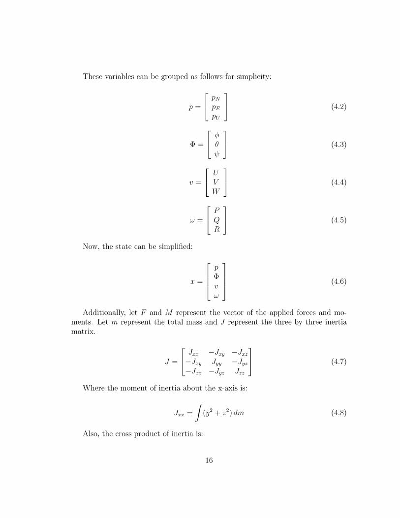
These variables can be grouped as follows for simplicity:

p =

pNpEpU

(4.2)

Φ =

φθψ

(4.3)

v =

UVW

(4.4)

ω =

PQR

(4.5)

Now, the state can be simplified:

x =

pΦvω

(4.6)

Additionally, let F and M represent the vector of the applied forces and mo-ments. Let m represent the total mass and J represent the three by three inertiamatrix.

J =

Jxx −Jxy −Jxz−Jxy Jyy −Jyz−Jxz −Jyz Jzz

(4.7)

Where the moment of inertia about the x-axis is:

Jxx =

∫(y2 + z2) dm (4.8)

Also, the cross product of inertia is:

16

Jxy ≡ Jyx =

∫xy dm (4.9)

Let Cb/i be the direction cosine matrix that will transfer a inertial frame vectorui to a body frame vector ub. The direction cosine matrix is made up of themultiplication of three seperate rotation matricies Cφ, Cθ and Cψ. Each of whichis a rotation about its own axis.

ub = Cb/i ui (4.10)

= CφCθCψ ui (4.11)

Since matrix multiplications do not commute, this implies a specific order to therotations. This order is yaw first, pitch second and roll third. This is the standardconvention in the aerospace industry.

Cφ =

1 0 00 cosφ sinφ0 − sinφ cosφ

(4.12)

Cθ =

cos θ 0 sin θ0 1 0

− sin θ 0 cos θ

(4.13)

Cψ =

cosψ sinψ 0− sinψ cosψ 0

0 0 1

(4.14)

Therefore,

Cb/i = cos(θ) cos(ψ) cos(θ) sin(ψ) − sin(θ)− cos(φ) sin(ψ) + sin(ψ) sin(θ) cos(ψ) cos(φ) cos(ψ) + sin(ψ) sin(θ) sin(ψ) sin(φ) cos(θ)sin(φ) sin(ψ) + cos(ψ) sin(θ) cos(ψ) − sin(φ) cos(ψ) + cos(ψ) sin(θ) sin(ψ) cos(φ) cos(θ)

(4.15)

17

4.1.1 Force Equations

The force equations will be derived from basic laws of physics. To begin, let Gbe the vector acceleration of gravity in the body fixed frame and g be the scalaracceleration due to gravity, which is approximately 9.8 meters per second squared.

G = Cb/i

00−g

=

g sin(θ)−g sin(φ) cos(θ)−g cos(φ) cos(θ)

(4.16)

From Newton’s second law, where the derivative is taken in the body frame:

F +mG =d

dtm v

= m (v + ω × v)(4.17)

Rearranging,

v =1

mF +G− ω × v (4.18)

4.1.2 Moment Equations

The moment equations can be derived in a similar method to the force equations.The state space equations for the derivative of angular velocity can be found byusing Newton’s second law for inertial systems.

M =d

dtJ ω (4.19)

Note that the derivative is taken in the inertial frame which results in thefollowing equation.

M = J ω + ω × J ω (4.20)

This equation can be rearranged to solve for the derivate of the state variables.

ω = J−1(M − ω × J ω) (4.21)

18

4.1.3 Navigation Equations

The navigation equations express a relationship between the positional derivatives pand the body fixed linear velocities v. This is done by rotating v using the directioncosine matrix to the inertial frame.

p = Cb/i v (4.22)

4.1.4 Kinematic Equations

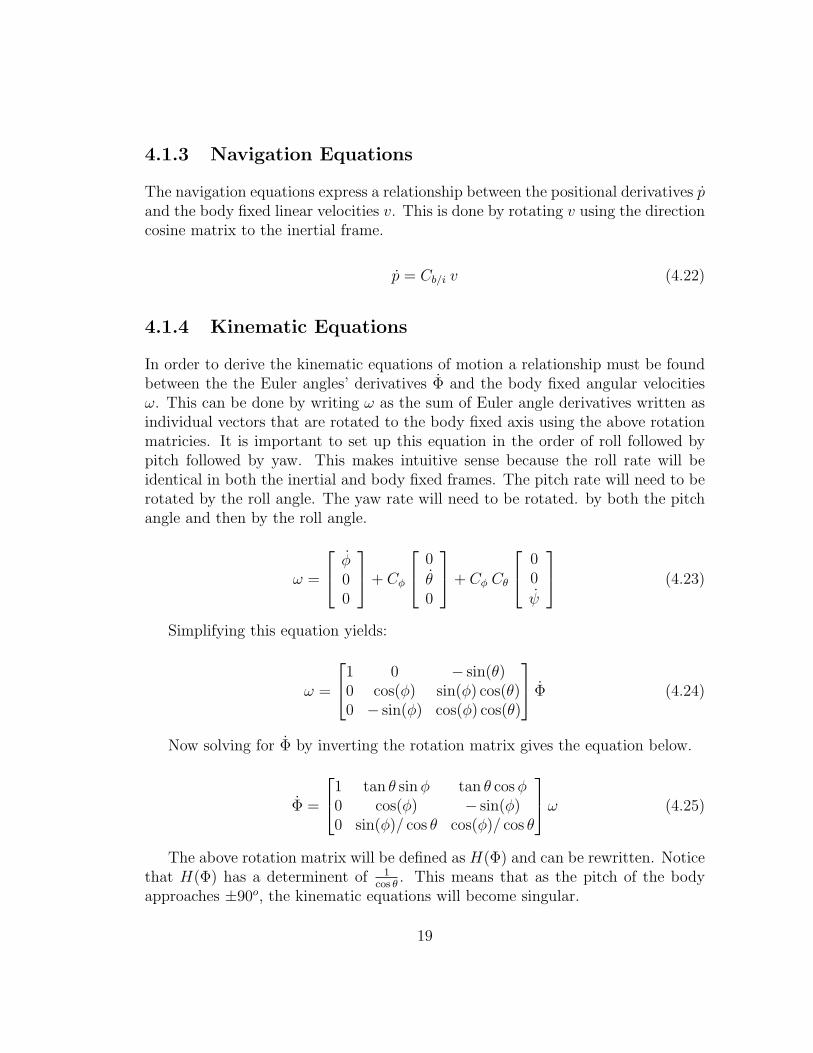
In order to derive the kinematic equations of motion a relationship must be foundbetween the the Euler angles’ derivatives Φ and the body fixed angular velocitiesω. This can be done by writing ω as the sum of Euler angle derivatives written asindividual vectors that are rotated to the body fixed axis using the above rotationmatricies. It is important to set up this equation in the order of roll followed bypitch followed by yaw. This makes intuitive sense because the roll rate will beidentical in both the inertial and body fixed frames. The pitch rate will need to berotated by the roll angle. The yaw rate will need to be rotated. by both the pitchangle and then by the roll angle.

ω =

φ00

+ Cφ

0

θ0

+ Cφ Cθ

00

ψ

(4.23)

Simplifying this equation yields:

ω =

1 0 − sin(θ)0 cos(φ) sin(φ) cos(θ)0 − sin(φ) cos(φ) cos(θ)

Φ (4.24)

Now solving for Φ by inverting the rotation matrix gives the equation below.

Φ =

1 tan θ sinφ tan θ cosφ0 cos(φ) − sin(φ)0 sin(φ)/ cos θ cos(φ)/ cos θ

ω (4.25)

The above rotation matrix will be defined as H(Φ) and can be rewritten. Noticethat H(Φ) has a determinent of 1

cos θ. This means that as the pitch of the body

approaches ±90o, the kinematic equations will become singular.

19

Φ = H(Φ) ω (4.26)

The above equation gives the kinematic relationship in the required form for astate space system.

4.1.5 Summary of Rigid Body Equations

Below is a summary of all of the rigid body equations needed for a state spacesimulation of a six degree of freedom system using aerospace conventions.

v =1

mF +G− ω × v (4.27)

ω = J−1(M − ω × J ω) (4.28)

p = Cb/i v (4.29)

Φ = H(Φ) ω (4.30)

20

4.2 Generation of Forces and Moments

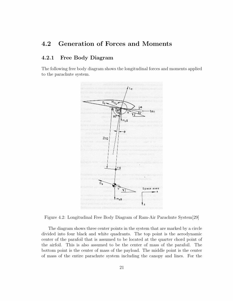
4.2.1 Free Body Diagram

The following free body diagram shows the longitudinal forces and moments appliedto the parachute system.

Figure 4.2: Longitudinal Free Body Diagram of Ram-Air Parachute System[29]

The diagram shows three center points in the system that are marked by a circledivided into four black and white quadrants. The top point is the aerodynamiccenter of the parafoil that is assumed to be located at the quarter chord point ofthe airfoil. This is also assumed to be the center of mass of the parafoil. Thebottom point is the center of mass of the payload. The middle point is the centerof mass of the entire parachute system including the canopy and lines. For the

21

purposes of this report it will be assumed that the mass of the canopy, mc and linesare negligible and that the center of mass of the parachute system is located at thecenter of mass of the payload. Therefore ms is equal to m.

A number of new angles are introduced in this diagram. The angle α representsthe angle of attack between the wind vector, V , and the parafoil chord. The angleγ represents the angle between the horizontal plane in the inertial reference frameand the wind vector experienced by the parafoil. Assuming there is no wind, thisis also the glide slope angle of the parafoil and V is identical to the previouslydefined velocity vector v. The rigging angle is labeled as tau in the diagram andwill denoted by τ .

The applied forces Lc and Dc refer to the lift and drag of the parafoil. Ds refersto the drag of the payload, which we will assume to be zero for simplicity. Mc/4 isthe aerodynamic pitching moment cause by the parafoil. The equations for parafoillift forces, drag forces and pitching moments can be written as follows [41].

Lc =1

2ρ V 2

T S CL (4.31)

Dc =1

2ρ V 2

T S CD (4.32)

Here ρ represents the density of air, VT represents the freestream velocity, S rep-resents the surface area of the parafoil and CL and CD represent the non-dimensionalcoefficients of lift and drag respectively. The coefficients of lift and drag vary forevery type and configuration of parafoil.

The variables that represent the aerodynamic moments for roll, pitch and yaware lw, mw and nw respectively. Their non-dimensional coefficients are Cl, Cm andCn, which also vary for different parafoils. The equations for these moments are asfollows.

lw =1

2ρ V 2

T S b Cl (4.33)

mw =1

2ρ V 2

T S c Cm (4.34)

nw =1

2ρ V 2

T S b Cn (4.35)

In the above equation b and c represent the wingspan and mean aerodynamicchord respectively.

22

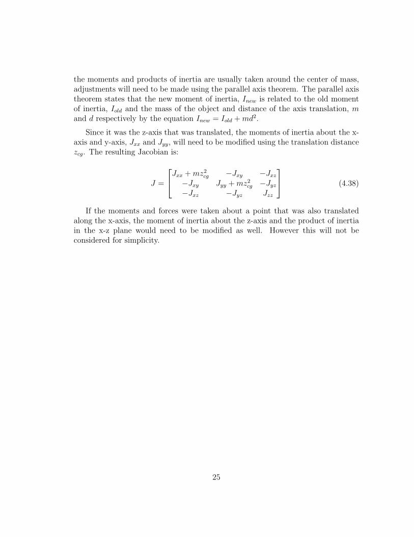
Obtaining accurate estimates of aerodynamic coefficients is an entire field ofstudy in and of itself. Theoretical and experimental studies have been performedto determine these parameters. Figure 4.3 shows the coefficient of lift for a ramair parafoil in a variety of aspect ratios. Figure 4.4 shows experimentally obtainedlongitudinal coefficients obtained from NASA’s X-38 program. This parachute sys-tem utilized a 15% thick Clark Y airfoil with an aspect ratio of 4.1 and a riggingangle of 13 degrees. Figure 4.5 and 4.6 shows the lateral coefficients from thesame study for various flap deflections (referred to as delta deflections) and riggingangles of 10 and 13 degrees. The variable δ in these figures refers to the increase indeflection on one side of the canopy.

Figure 4.3: Ram Air Parafoil Coefficient of Lift for Various Aspect Ratios[29]

Figure 4.4: Longitudinal Aerodynamic Coefficients[22]

The previously rigid body equations used F and M to refer to the forces andmoments applied to the rigid body. These forces and moments will be taken about

23

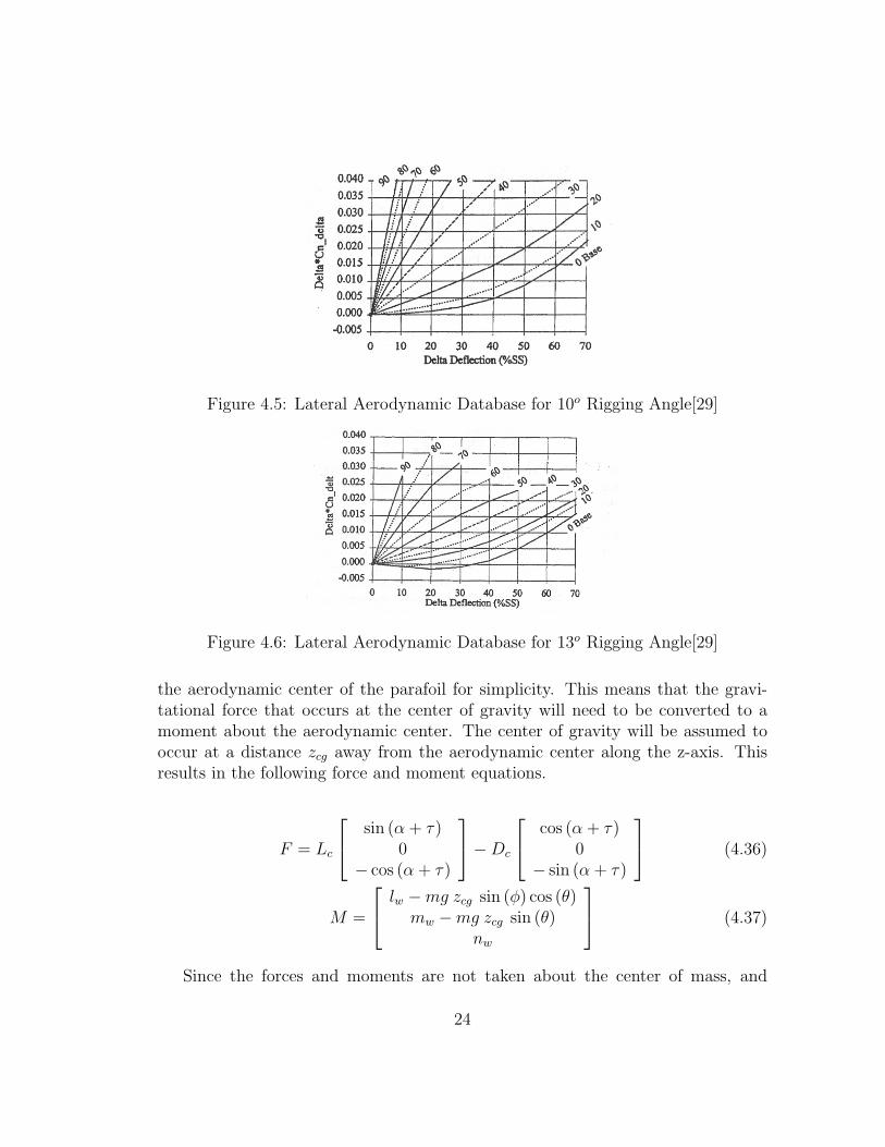
Figure 4.5: Lateral Aerodynamic Database for 10o Rigging Angle[29]

Figure 4.6: Lateral Aerodynamic Database for 13o Rigging Angle[29]

the aerodynamic center of the parafoil for simplicity. This means that the gravi-tational force that occurs at the center of gravity will need to be converted to amoment about the aerodynamic center. The center of gravity will be assumed tooccur at a distance zcg away from the aerodynamic center along the z-axis. Thisresults in the following force and moment equations.

F = Lc

sin (α+ τ)0

− cos (α+ τ)

−Dc

cos (α+ τ)0

− sin (α+ τ)

(4.36)

M =

lw −mg zcg sin (φ) cos (θ)mw −mg zcg sin (θ)

nw

(4.37)

Since the forces and moments are not taken about the center of mass, and

24

the moments and products of inertia are usually taken around the center of mass,adjustments will need to be made using the parallel axis theorem. The parallel axistheorem states that the new moment of inertia, Inew is related to the old momentof inertia, Iold and the mass of the object and distance of the axis translation, mand d respectively by the equation Inew = Iold +md2.

Since it was the z-axis that was translated, the moments of inertia about the x-axis and y-axis, Jxx and Jyy, will need to be modified using the translation distancezcg. The resulting Jacobian is:

J =

Jxx +mz2cg −Jxy −Jxz

−Jxy Jyy +mz2cg −Jyz

−Jxz −Jyz Jzz

(4.38)

If the moments and forces were taken about a point that was also translatedalong the x-axis, the moment of inertia about the z-axis and the product of inertiain the x-z plane would need to be modified as well. However this will not beconsidered for simplicity.

25

4.3 Apparent Mass Effects

When an object travels through a vacuum, the forces acting upon it are directlyrelated to the object’s acceleration using Newton’s Second Law, F = ma. Whenan object is traveling through a fluid it causes the fluid to move. If the motionof the object is to change, it must change the movement of the fluid as well. Theexisting fluid motion resists this change by applying a pressure on the body. Thispressure is proportional to the object’s acceleration and can be expressed as anincrease in the object’s mass, mAM such that Newton’s second law is changed toF = (m+mAM)a [30].

Most people have experienced this effect while holding their hand out of a carwindow that is driving at highway speeds. If a person’s hand is positioned horizon-tally there will be no turbulence and the apparent mass effect will be noticeable.The person’s hand will not feel a great deal of drag pushing their hand back, how-ever translating their hand up or down in the airstream requires a great deal offorce (assuming they are not changing the angle of attack). To this person it wouldfeel as if their hand is much heavier than it actually is. This is the apparent masseffect.

It is important to note that all airplanes experience the apparent mass effect;however for heavy wing loadings, such as those of an airplane, the apparent masseffect is negligible. For light wing loadings (less than five kilograms per squaremeter) such as a parafoil [30].

Lissaman [30] outlines six apparent mass terms; A, the surge term, B, the side-slip term, C, the plunge term, IA, the roll term, IB the pitch term and IC , the yawterm. The applied forces and moments due to the apparent mass terms are definedas follows.

26

F1 = −A∂U∂t

− CWq +BV r (4.39)

F2 = −B∂V∂t

− AUr + CWp (4.40)

F3 = −C∂W∂t

−BV p+ AUq (4.41)

M1 = −IA∂p

∂t− (IC − IB)qr − (C −B)WV (4.42)

M2 = −IB∂q

∂t− (IA − IC)rp− (A− C)UW (4.43)

M3 = −IC∂r

∂t− (IB − IA)pq − (B − A)V U (4.44)

(4.45)

We can simplify these equations by grouping terms.

FAM = [F1, F2, F3]T (4.46)

MAM = [M1,M2,M3]T (4.47)

KABC =

A 0 00 B 00 0 C

(4.48)

KIAIBIC =

IA 0 00 IB 00 0 IC

(4.49)

Now,

FAM = −KABC v − ω × (KABC v) (4.50)

MAM = −KIAIBIC ω − ω × (KIAIBIC ω)− v × (KABC v) (4.51)

As a result, the applied force, F , and moment, M , acting on the body is a sumof the apparent mass forces and moments as well as the aerodynamic forces andmoments, which are denoted by Faero andMa. This is expressed as: F = Faero+FAMandM = Maero+MAM . Substituting these results into the force equation (Equation4.18) results in the following.

27

v =1

m(Faero −KABC v − ω × (KABC v)) +G− ω × v (4.52)

(I +1

mKABC)v =

1

mFaero +G− ω × (v +

1

m(KABC v)) (4.53)

v = (I +1

mKABC)−1(

1

mFaero +G− ω × (v +

1

m(KABC v))) (4.54)

Similarly the moment equation (Equation 4.21) can be modified.

ω = J−1(Maero −KIAIBIC ω − ω × (KIAIBIC ω)− v × (KABC v)− ω × J ω)(4.55)

(I + J−1KIAIBIC )ω = J−1(Maero − ω × (KIAIBIC ω)− v × (KABC v)− ω × J ω)(4.56)

ω = (I + J−1KIAIBIC )−1J−1(Maero − ω × (KIAIBIC ω)− v × (KABC v)− ω × J ω)(4.57)

ω = (J +KIAIBIC )−1(Maero − ω × (KIAIBIC ω)− v × (KABC v)− ω × J ω) (4.58)

Lissaman [30] approximates the shape of the parafoil with a number of cylin-ders and generates equations for the six apparent mass terms using the simplifiedgeometry. The geometry and variables used are shown in Figures 4.7 and 4.8. Therelevant equations are listed in Equations 4.59 through 4.64.

A = 0.899π

4t2b (4.59)

B = 0.39π

4(t2 + 2α2)c (4.60)

C = 0.783π

4c2b (4.61)

IA = 0.630π

48c2b3 (4.62)

IB = 0.8174

48πc4b (4.63)

IC = 1.001π

48t2b3 (4.64)

28

Figure 4.7: Parafoil Geometry[30]

Figure 4.8: Volumetric Representations of Apparent Mass and Moments[30]

29

4.4 Wind Disturbances

The rigid body equations previously discussed assumed that the vehicle is travelingin an environment with no wind. However, wind can have a significant effect on aparachute. All types of wind can be modeled by a velocity vector that can changeover time. Let vwind denote the wind velocity vector in the inertial frame. Therigid body equations can be modified to include wind disturbances by also solvingan additional equation to relate v with the relative air velocity vrel experienced bythe parachute. The relationship between these variables is as follows [41].

vrel = v − Cb/i vwind (4.65)

Where vrel = [U ′, V ′,W ′]T .

A variety of wind models can be used, the simplest being a constant wind thathas only a DC component. Accurate representations of gusting winds model thewind velocity as a random process, such as white Gaussian noise. More complexmodels will filter the white Gaussian noise to get a specific frequency responsethat is a function of turbulence intensity, turbulence scale length, altitude andother parameters. Examples of these more complex wind models can be found inmilitary specifications for handling qualities[34].

It should be noted that when there is no wind present, the angle of attack, α isequivalent to the glide slope ratio, γ.

30

4.5 Sensor Dynamics

For the purposes of this report, it will be assumed that the sensors are perfect,with the exception that they add zero-mean white Gaussian noise to any measuredquantities. Therefore each measured quantity will be described by its own noisevariance σ.

31

4.6 Parachute System Parameters

The six degree of freedom simulation has been simulated in Matlab. The fullstate matrix described above was solved using the fourth order Runge-Kutta (RK4)algorithm. The input to the system was modeled as a braking deflection and asa differential deflection. and the output of the system is its state. The followingparameters were chosen (all variables are in metric units) based on values takenfrom a number of papers [21, 22, 40] and are shown in Table 4.1. These valueswere not taken using actual data from a single parachute system, therefore thesimulations will not be exact.

Variable Description Valueg gravity 9.81ρ density of air 1.2a parafoil height 0.9144b parafoil span 2.1336c parafoil chord 0.6096S planform area 1.3t thickness 0.127zcg C.O.M. Offset 1.2192τ rigging angle 1.3m mass of vehicle 4.0Jxx Moment of Inertia 6.1298Jyy Moment of Inertia 6.150Jzz Moment of Inertia 0.02752Jxy Product of Inertia 0.0Jxz Product of Inertia 0.00339Jyz Product of Inertia 0.0

Table 4.1: Simulator Parameter Values

The aerodynamic coefficients were approximated from previously shown charts.Note that V 2

T = v · v, and that δf and δa represent the control inputs for flaps andailerons respectively (which are combined as flaperons in the physical system).

32

CL = CLo + CLα α+ CLδfδf (4.66)

CD = CDo + CDα α+ CDδfδf + CD

δ2f

δ2f (4.67)

Cm = Cmo + Cmα α+ Cmδfδf + Cm

δ2f

δ2f (4.68)

Cn =b

2 VTCnR

R + Cnδaδa (4.69)

Cl = 0 (4.70)

The selected values for these aerodynamic coefficients are shown in Table 4.2.

Variable ValueCLo 0.2CLα 0.0375CLδf

0.377

CDo 0.12CDα 0.0073CDδf

0.076

CDδ2f

0.266

Cmo -0.0115Cmα -0.004Cmδf

0.16

Cmδ2f

0.056

CnR-0.0936

Cnδa0.05

Table 4.2: Aerodynamic Coefficient Values

33

4.7 Simulation Results

The six degree of freedom simulations were performed using the simulation filesfound in Appendix B. These files implement the equations discussed in this chapterwith one exception. For an unknown reason the v × (KABC v) in Equation 4.58,would cause an unstable pitching moment in the system. All of the equationsand parameters seem to be similar to those found in literature references[21, 22,41]. However not all papers include the non-linear apparent mass terms, evenwhen performing a non-linear simulation, such as Slegers [40]. The reason for thisvariation was not found during the course of this project. Removing this part ofthe equation generated the expected results; however this is indicative that furtherinvestigation is needed for precise dynamic simulation.

In the first set of diagrams, Figure 4.9 shows that no control input is appliedand shows appropriate and expected results. Figure 4.10 shows the parachute glidesforwards and downwards with a glide slope ratio of 2.5:1. Figure 4.11 shows thatU , V and W stabilize at approximately 10, 0 and 3 meters per second respectively.Figure 4.12 illustrates the fact that the pitch oscillates and settles to a constant pitchof negative three degrees after 10 seconds, while Figure 4.13 shows the expectedangular rates. Figure 4.14 and 4.15 show that within six seconds the angle of attackand net velocity settle to five degrees and 11 meters per second respectively.

Figure 4.9: No Control Input

The second simulation shows the response to a full brake deflection for 15 sec-

34

Figure 4.10: No Control Input: XYZ Position - North, East, Up (m)

onds. The figures show that the glide slope ratio is decreased, and the pitch isincreased, which is consistent with this type of a flare maneuver.

35

Figure 4.11: No Control Input: XYZ Velocity - Body Fixed Axis (m/s)

Figure 4.12: No Control Input: Euler Angles (degrees)

36

Figure 4.13: No Control Input: Angular Rates (degrees per second

Figure 4.14: No Control Input: Angle of Attack (degrees)

37

Figure 4.15: No Control Input: Net Velocity (m/s)

Figure 4.16: Braking Control Input

38

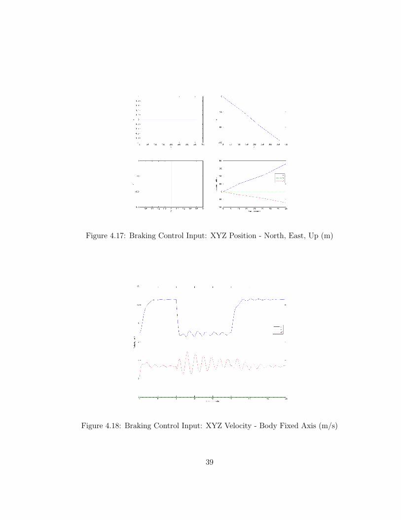
Figure 4.17: Braking Control Input: XYZ Position - North, East, Up (m)

Figure 4.18: Braking Control Input: XYZ Velocity - Body Fixed Axis (m/s)

39

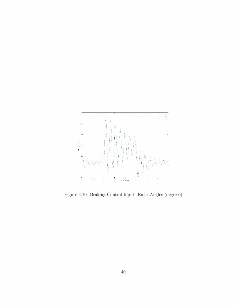
Figure 4.19: Braking Control Input: Euler Angles (degrees)

40

Chapter 5

Nine Degree of FreedomSimulation

The six degree of freedom model restricts the parafoil and payload to be fixed inposition and orientation with respect to each other. However, the physical systemconnects the parafoil and payload using strings. These strings can twist and stretchallowing the bodies to be at different relative positions and orientations.

A nine degree of freedom model has been used to allow changes in relativeorientations [22, 21]. A nine degree of freedom model can be constructed using twosix degree of freedom models that are constrained with each other. This wouldresult in 12 equations of motion and 3 constraint equations.

For the parachute system, the constraint equations would describe a sphericaljoint constraint that would fix locations on the two bodies with respect to eachother. Additionally, forces would be added to both bodies with respect to their rel-ative orientations simulating a spring-damper system. This means that in steadystate conditions the nine degree of freedom model would be identical to the six de-gree of freedom model. However during transient flight, this would not be the case.The difference in orientation would be relative to the tension and inelasticity in thecanopy lines. Larger canopies would experience a greater difference in orientationduring gusting winds because the payload and parafoil are less likely to experiencethe same winds.

Numerous textbooks [20, 18] describe methods for setting up kinematic con-straint equations. These textbooks do not use the aerospace conventions where thestate vector includes body fixed velocities, but rather use the velocities in the iner-tial frame. Since these constraints are positional constraints written in the inertial

41

frame, their derivatives will also be in the inertial frame, which is incompatiblewith the aerospace conventions. These equations can be modified to work withaerospace conventions, but due to the difficulty of this problem and the minimal ofbenefit of the results, a nine degree of freedom model will not be implemented.

42

Chapter 6

Guidance, Navigation and ControlSystem Design

The guidance, navigation and control system are designed to force the parachute tofollow as accurate of a specified path as possible. The relationship between thesesystems can be seen in Figure 6.1.

Figure 6.1: Guidance, Navigation and Control System

The navigation system measures and estimates all of the relevant states, x, ofthe vehicle by measuring the plant output, y. The elements of x are the full set ofnon-linear states, x = [pN , pE, pU , φ, θ, ψ, U, V,W, P,Q,R]T and y is the state vectoras seen by the sensor system and will not be further discussed. The path databasestores the path, p, that the parachute must follow. The sequence of p is representedby an array of positions in the inertial frame. The guidance system uses the pathdatabase to generate a reference signal, r, which will be discussed in the guidance

43

section. The control system is then used to track that reference signal by applyinga control input u to the plant.

44

6.1 Guidance System

The purpose of the guidance and control system is to force the parachute to followa specified path. The control system’s job is to make the state variables of theparachute track specified commands. The guidance system is responsible for gen-erating these commands based on a desired trajectory. This trajectory can eitherbe pre-programmed or generated in real time. In this section, a methodology isproposed for storing a trajectory and using this trajectory to generate signals forthe control system. It is important to note that one of the fundamental limitationsof a parachute is that its altitude is always decreasing. The guidance system mustbe designed with this constraint in mind.

In the proposed guidance system, the desired trajectory will be represented bya single path, in the inertial frame, from the minimum altitude to the maximumaltitude. It is likely that in the final system, some part of the path will go throughthe location of the open window in the building. Additionally, the maximum alti-tude should be greater that the altitude at which the parachute is deployed so thatit always has a path to follow.

There are a number of constraints on this trajectory. The first constraint isthat every altitude in between will have a single point on that path. There cannotbe two points at the same altitude. The second constraint requires the path to befully continuous, there can be no discontinuities. The third and most significantconstraint is that at all points on this path, the glide slope must be less than orequal to the maximum possible glide slope for the parachute.

A lookup function, Γ, will be used to determine the location of a point on thepath at a given altitude, h. An example of this function is below: pN

pEpU

= Γ(h) (6.1)

Although any data structure can be used for this lookup function it is suggestedthat the path is represented by an array of connected straight lines (rather thancurved lines) that have different directions and glide slopes. Each element in thearray would represent a straight line that exists in a vertical section of the airspace,and data points could be quickly and easily generated from this.

To follow the trajectory, the guidance system must generate signals that leadthe parachute onto its path. The proposed method aims the parachute at a pointon the trajectory that is at a lower altitude. The difference between the parachute’s

45

current altitude and the lower altitude is a fixed constant ka. This constant canbe tuned experimentally to obtain the best performance. The location of theparachute is [pNp , pEp , pUp ]

T . The location of the point that should be aimed forcan is [pNn , pEn , pUn ]T , and can be determined by: pNn

pEn

pUn

= Γ(h− ka) (6.2)

The guidance system will aim the parachute at its trajectory by generating twosignals to be tracked, the desired track over ground, ψg, and the desired glide sloperatio, U

V. The following equations can be used to generate these signals:

ψg = arctan(pEn − pEp

pNn − pNp

) (6.3)

U

V=

√(pNn − pNp)

2 + (pEn − pEp)2

pUp − pUn

(6.4)

For this reason, the control system’s inputs must accept a track over groundand a glide slope ratio.

46

6.2 Navigation

The navigation system is used for measuring the state of the system. At a minimum,this system must generate sufficiently accurate measurements for the guidance andcontrol system to use. This implies that the navigation system must be capableof measuring the position of the parachute in the inertial frame, the glide slope inthe body frame and the track of the parachute in the inertial frame. Due to timeconstraints the detailed design of a navigation system is outside of the scope of thisreport. However, suggestions for the sensors and some mandatory requirements ofthe navigation system will be outlined.

A Global Positioning System (GPS) and Attitude Heading Reference System(AHRS) would be sufficient to estimate the state of the parachute to be provided tothe guidance and control systems. The GPS can provide certain variables directly,[pN , pE, pU , ˙pN , pE, pU ], while the AHRS can provide [φ, θ, ψ, P,Q,R]. With thesetwo systems, simple rotations can be used to calculate [U, V,W ] from the GPS andAHRS. These variables can be used to calculate the glide slope ratio U

Vand track

over ground arctan(W/U).

When designing the guidance system, a number of problems will arise. The mea-surements from the GPS receiver will normally have a 0.5 second delay, whereasa typical AHRS delay will be less than 0.01 seconds. This difference must beaccounted for since this is a high precision application. Bias instabilities in thegyroscopes on the AHRS will cause its data to drift over time if the system is un-dergoing constant accelerations, which are unavoidable in any aerial vehicle. Somelow cost AHRS systems that use micro-electromechanical (MEMS) vibrating gyro-scopes have very high bias instabilities. This can mean that the AHRS is unusableafter 30 seconds. To correct this, GPS acceleration measurements should be sub-tracted from the accelerometers’ measurements before the AHRS’s algorithms arerun[42].

Additional last minute trajectory corrections must be made due to the fact thatthe location of the open window is likely to be highly inaccurate. This is becausethe airplane that dropped the parachute will have located the window using itsonboard camera and projected the windows location to the inertial frame usingthe airplane’s location and orientation. Any error in the attitude of the aircraftwill be amplified by the distance that the plane is away from the window. Roughcalculations for typical inaccuracies and problem geometries show that the finalmeasurement may be off by as much as four to six meters. It is recommendedthat a sensor, such as an image processing system, should be used to correct thetrajectory when the parachute is closer to the window. The design of this type of

47

system is well outside the scope of this report and will not be discussed further.

48

6.3 Linearization

The six degree of freedom dynamic model previously discussed is a non-linear model.Since the control system will not be designed using non-linear techniques, thismodel must be linearized. Additionally, the state vector described in the previouschapters does not include the glide slope ratio or track over ground, which is whatthe control system must track. In order to deal with this, some adjustments needto be made. The adjustment is to assume that there is no wind. This will obviouslycause problems when gusting winds are present. However, over the long term, theguidance system will make the necessary corrections because it is tracking the pathin the inertial frame rather than the body frame.

When there is no wind, the glide slope ratio is equal to the angle of attack,and the track over ground is equal to the yaw angle. Since, the angle of attackis not part of the state vector, the system equations will need to be translatedto an equivalent set of system equations that uses the angle of attack as one ofits state variables. An extra benefit of this is that this new system will make theaerodynamic coefficients easier to linearize. These steps will be fully explained laterin this section.

In a linear model, the derivatives of the state vector must be written as a linearcombination of the state variables themselves as well as the input variables. Theelements of the matrices A and B are the coefficients of these linear combinations.The common notation for this type of linear system is:

x = Ax+Bu (6.5)

Since the parachute’s velocity is not constant, linearizing around a certain posi-tion would yield catastrophic results. Therefore, the navigation equations are takenout of the state equations. In simulation, these equations are still used; however,they can not be used to generate the controller.

The process of linearizing a dynamic model requires an equilibrium state tobe selected. The linearized model will only be accurate when the system’s stateis close to the equilibrium state. The following approximations represent part ofthe selected equilibrium state. The equilibrium positions of the remaining statevariables will be outlined later in this section.

49

P ≈ 0 (6.6)

Q ≈ 0 (6.7)

R ≈ 0 (6.8)

φ ≈ 0 (6.9)

θ ≈ θ0 (6.10)

These approximations imply that the vehicle is close to straight and level flightconditions. The parachute is not banked and has no angular velocity about anyaxis. However, it does have a nominal pitch.

No equilibrium position for ψ was selected because it is not desirable to limitthe heading to a small range. The heading can normally fall in the range of 0 to360 degrees. Normally it is not possible to create a linear system without selectingan equilibrium point for all of the variables. However, in this case it is possible tocreate a linear system without selecting an equilibrium point for φ because none ofthe state equations depend on ψ. This makes intuitive sense, because the dynamicsof a parachute do not change depending direction in which it is traveling.

Additionally, equilibrium points for the variables U , V andW were not included.The reason for this is that it is very difficult to write the aerodynamic coefficientsin terms of linear combinations of v. For this reason, it is recommended [41] toreplace these variables with three different variables that provide essentially thesame information. These variables are the net airspeed VT , the angle of attack, α,and the sideslip angle β. This also provides the state variables that the controlsystem must track in the no wind condition. The definitions of these variables areprovided in the following equations:

VT =√vTrel · vrel (6.11)

α = arctan (W ′U ′

) (6.12)

β = arcsin (V ′VT

) (6.13)

The force equations must be altered to use the state variables [VT , α, β]T . Stevensand Lewis [41] provide a method to do this using a new reference frame called thewind and stability axes. The stability frame is found by rotating the body fixed

50

frame through the angle of attack. The wind frame is then found by rotating thestability frame through the sideslip angle. Now, a few additional variables must bedefined. The variables g1, g2 and g3 represent the gravity vector in the wind frame.

g1 = g (− cos (α) cos (β) cos (θ)

+ sin (β) sin (φ) cos (θ)

+ sin (α) cos (β) cos (φ) cos (θ)) (6.14)

g2 = g (cos (α) sin (β) sin (θ)

+ cos (β) sin (φ) cos (θ)

− sin (α) sin (β) cos (φ) cos (θ)) (6.15)

g3 = g (sin (α) sin (θ) + cos (α) cos (φ) cos (θ)) (6.16)

Also, the rotation matrix from the body to wind axes is Cw/b.

Cw/b =

cos(α) cos(β) sin(β) − sin(α) cos(β)cos(α) sin(β) cos(β) − sin(α) sin(β)

sin(α) 0 − cos(α)

(6.17)

One other change is that the rotation rates are defined in the stability axes.Therefore the state vector includes ωs = [Ps, Q,Rs]

T . As you can see, the rotationaround the y-axis of the parachute did not change the value of Q.

After modifying the equations to suit the parafoil system, the following equa-tions are the result.

m

VTβ VT

α VT cos(β)

= Cw/b

F1

F2

F3

− D

0L

+m

g1

g2

g3

−mVT

0Rs

Q cos(β)− Ps sin(β)

(6.18)

Now the moment equations will need to be expressed in terms of the stability axisequations. Again, Stevens and Lewis provide the derivation of these equations [41].

51

First, the inertia tensor must be redefined in the stability axis. The components ofthis matrix are Jxx′, Jzz′ and Jxz′.

Jxx′ = (Jxx +mz2cg) cos2(α) + Jzz sin2(α)− Jxz cos(2α) (6.19)

Jzz′ = (Jxx +mz2cg) sin2(α) + Jzz cos2(α) + Jxz cos(2α) (6.20)

Jxz′ = 0.5(Jxx +mz2cg − Jzz) sin(2α) + Jxz cos(2α) (6.21)

This is used in generating a new inertia tensor, Js.

Js =

Jxx′ 0 −Jxz′0 Jyy +mz2

cg 0−Jxz′ 0 Jzz′

(6.22)

This results in a new set of moment equations.

m

PsQ

Rs

= −α

−Rs

0Ps

+ J−1s (M − ω × Js ω) (6.23)

Once the apparent mass effects are included, the force equation becomes:

m

VTβ VT

α VT cos(β)

= Cw/b (−KABC v − ω × (KABC v))−

D0L

+m

g1

g2

g3

−mVT

0Rs


(6.24)

(m+KABC)

VTβ VT

α VT cos(β)

= −

D0L

+m

g1

g2

g3

− (m+ A)VT

0Rs


(6.25)

52

Next the moment equation becomes:

PsQ

Rs

= −α

−Rs

0Ps

+ J−1s (Maero −KIAIBIC ω − ω × (KIAIBIC ω)

− v × (KABC v)− ω × Js ω) (6.26)

(Js +KIAIBIC )

Ps − αRs

Q

Rs + αPs

= Maero −

PsQRs

× IAPsIBQICRs

−

VTVT sin(β)

0

× AVTBVT sin(β)

0

− PsQRs

× Js

PsQRs

(6.27)

Now a few more approximations can be made for the linearization process. Thefirst two assumptions follow directly from P ≈ 0 and R ≈ 0. The variable VT0 isthe nominal airspeed of the parachute and the variable α0 is an equilibrium angle ofattack for the system that is normally between 0 and 15 degrees. The assumptionthat β is zero implies that there is no sustained side slip.

Ps ≈ 0 (6.28)

Rs ≈ 0 (6.29)

VT ≈ VT0 (6.30)

α ≈ α0 (6.31)

β ≈ 0 (6.32)

The process of linearzing a non-linear model creates a small perturbation system.The details of how the linearization process works will not be discussed in thisreport. However, if the reader is unfamiliar with this process there are a numberof textbooks that provide the full explanations of the linearization process[17, 4].

Now the dynamic equations with the state vector x = [VT , β, α, φ, θ, ψ, Ps, Q,Rs]T

will be linearized about the operating point x0 = [VT0 , 0, 0, 0, 0, ψ, 0, 0, 0]T . Smallchanges in variables will be denoted by being preceded by ∆. To begin, the kine-matic equations, Equations 4.26, are linearized as follows.

53

∆φ = ∆Ps + ∆Rs tan(θ0) (6.33)

∆θ = ∆Q (6.34)

∆ψ = ∆R1

cos(θ0)(6.35)

Next, the force equations, Equations 6.25, are linearized as follows. Note thatCDX0

represents the drag coefficient evaluated at the equilibrium point and thatthe rate of change of the angle of attack is approximately zero.

(m+ A) ∆VT =− ρVT0SCDo ∆VT

− 1

2ρV 2

T0SCDα ∆α

− 1

2ρV 2

T0SCDδf

∆δf

+mg (sin(α0) sin(θ0) + cos(α0) cos(θ0)) ∆α

−mg (sin(α0) sin(θ0) + cos(α0) cos(θ0)) ∆θ

(6.36)

(m+B)VT0 ∆β =− ρVT0SCDo ∆VT

+mg (cos(α0) sin(θ0)− sin(α0) cos(θ0)) ∆β

−mg cos(θ0) ∆φ

− (m+ A)VT0 ∆Rs

(6.37)

(m+ C)VT0 ∆α =− ρVT0SCLo ∆VT

− 1

2ρV 2

T0SCLα ∆α

− 1

2ρV 2

T0SCLδf

∆δf

+mg (cos(α0) sin(θ0)− sin(α0) cos(θ0)) ∆α

+mg (sin(α0) cos(θ0)− cos(α0) sin(θ0)) ∆θ

(6.38)

Now the moment equations are linearized:

54

∆Ps =

(12(Jxx − Jzz + IA − IC +mz2

cg) sin(2α0) + Jxz cos(2α0)

(Jxx + IA +mz2cg)(Jzz + IC)− J2

xz

)(

1

2ρV 2

T0bCnRs

∆Rs +1

2ρV 2

T0bCnδa

∆δa − (B − A)V 2T0

∆β

)(6.39)

∆Q =

(Jyy +mz2

cg

(Jxx+ IA +mz2cg)(Jzz + IC)− J2

xz

)(ρVT0cCmo ∆VT +

1

2ρV 2

T0bCmα ∆α+

1

2ρV 2

T0bCmδf

∆δf

)(6.40)

∆Rs =

((Jxx + IA +mz2

cg) cos2(α0) + (Jzz + IC) sin2(α0)− Jxz sin(2α0)


xz

)(

1

2ρV 2

T0bCnRs

∆Rs +1

2ρV 2

T0bCnδa

∆δa − (B − A)V 2T0

∆β

)(6.41)

The linearized equations can now be written in matrix form. As previouslystated the state and input variables are x = [VT , β, α, φ, θ, ψ, Ps, Q,Rs]

T and u =[δf , δa]

T .

∆x = A∆x + B ∆u (6.42)

A =

A11 0 A13 0 A15 0 0 0 0A21 A22 0 A24 0 0 0 0 A29

A31 0 A33 0 A35 0 0 0 00 0 0 0 0 0 A47 0 A49

0 0 0 0 0 0 0 A58 00 0 0 0 0 0 0 0 A69

0 A72 0 0 0 0 0 0 A79

A81 0 A83 0 0 0 0 0 00 A92 0 0 0 0 0 0 A99

(6.43)

55

B =

B11 00 0B31 00 00 00 00 B72

B81 00 B92

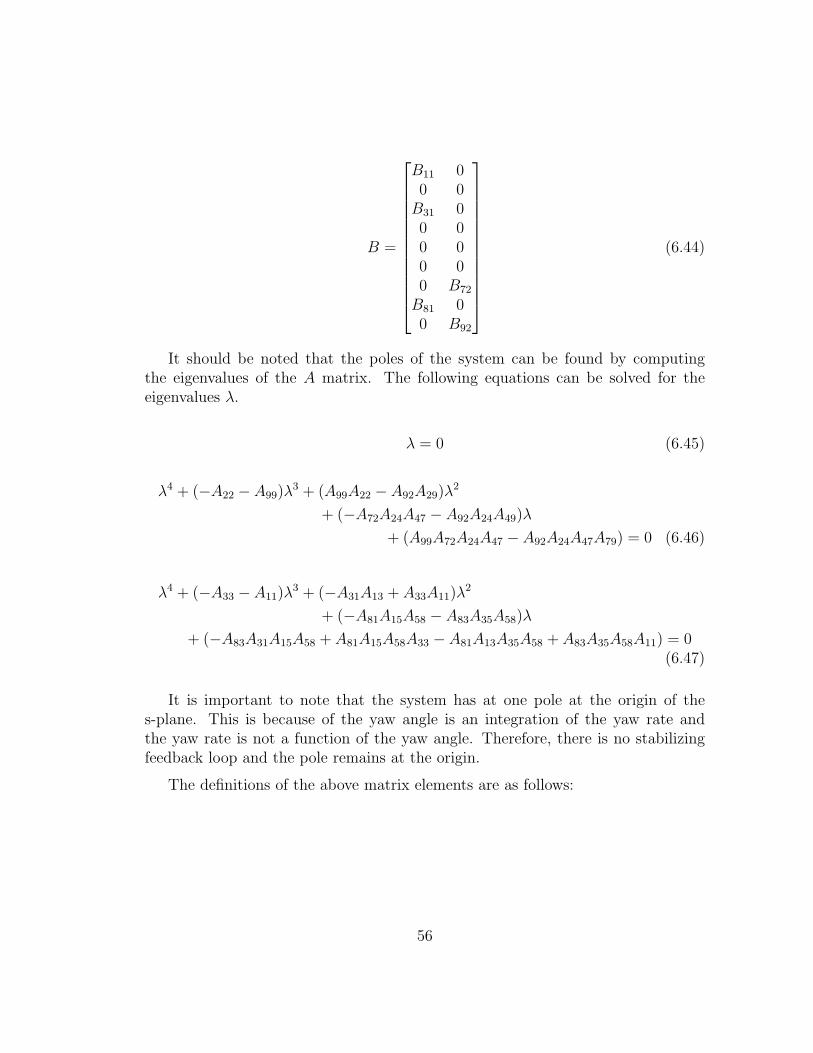
(6.44)

It should be noted that the poles of the system can be found by computingthe eigenvalues of the A matrix. The following equations can be solved for theeigenvalues λ.

λ = 0 (6.45)

λ4 + (−A22 − A99)λ3 + (A99A22 − A92A29)λ

2

+ (−A72A24A47 − A92A24A49)λ

+ (A99A72A24A47 − A92A24A47A79) = 0 (6.46)

λ4 + (−A33 − A11)λ3 + (−A31A13 + A33A11)λ

2

+ (−A81A15A58 − A83A35A58)λ

+ (−A83A31A15A58 + A81A15A58A33 − A81A13A35A58 + A83A35A58A11) = 0(6.47)

It is important to note that the system has at one pole at the origin of thes-plane. This is because of the yaw angle is an integration of the yaw rate andthe yaw rate is not a function of the yaw angle. Therefore, there is no stabilizingfeedback loop and the pole remains at the origin.

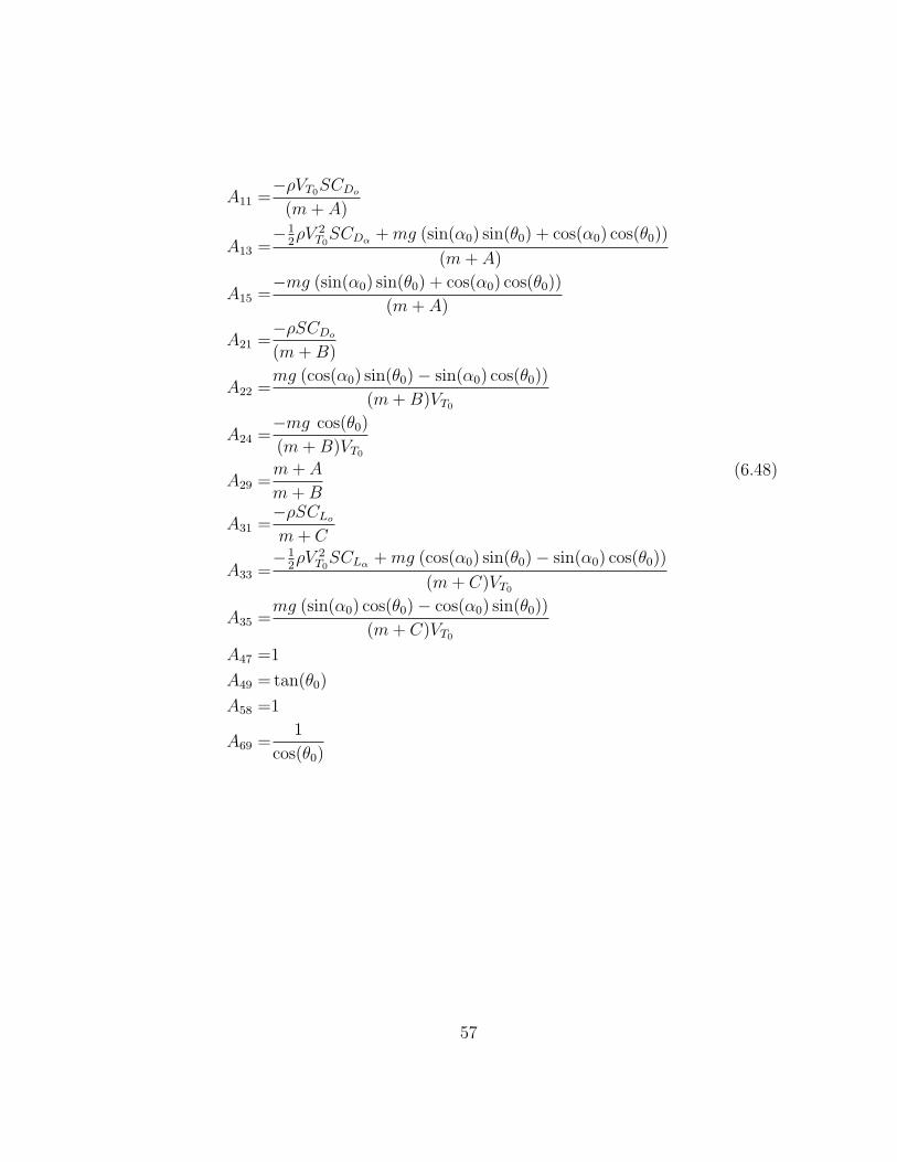
The definitions of the above matrix elements are as follows:

56

A11 =−ρVT0SCDo

(m+ A)

A13 =−1

2ρV 2

T0SCDα +mg (sin(α0) sin(θ0) + cos(α0) cos(θ0))

(m+ A)

A15 =−mg (sin(α0) sin(θ0) + cos(α0) cos(θ0))

(m+ A)

A21 =−ρSCDo

(m+B)

A22 =mg (cos(α0) sin(θ0)− sin(α0) cos(θ0))

(m+B)VT0

A24 =−mg cos(θ0)

(m+B)VT0

A29 =m+ A

m+B

A31 =−ρSCLo

m+ C

A33 =−1

2ρV 2

T0SCLα +mg (cos(α0) sin(θ0)− sin(α0) cos(θ0))

(m+ C)VT0

A35 =mg (sin(α0) cos(θ0)− cos(α0) sin(θ0))

(m+ C)VT0

A47 =1

A49 = tan(θ0)

A58 =1

A69 =1

cos(θ0)

(6.48)

57

A72 =




xz

)(−(B − A)V 2

T0

)A79 =




xz

)(1

2ρV 2

T0bCnRs

)A81 =

(Jyy +mz2

cg


xz

)(ρVT0cCmo)

A83 =

(Jyy +mz2

cg


xz

)(1

2ρV 2

T0cCmα

)A92 =

((Jxx + IA +mz2



xz

)(−(B − A)V 2

T0

)A99 =

((Jxx + IA +mz2



xz

)(

1

2ρV 2

T0bCnRs

)(6.49)

B11 =−1

2ρV 2

T0SCDδf

m+ A

B31 =−1

2ρV 2

T0SCLδf

m+ C

B72 =




xz

)(1

2ρV 2

T0bCnδa

)B81 =

(Jyy +mz2

cg


xz

)(1

2ρV 2

T0cCmδf

)B92 =

((Jxx + IA +mz2



xz

)(1

2ρV 2

T0bCnδa

)(6.50)

58

6.4 System Identification

Up until this point, the numerical values for parameters in the parachute system’sdynamic model have been based on crude estimates and comparisons with publishedresults and static measurements. No data from dynamic experiments have beentaken. For this reason, there is a great deal of model uncertainty with the dynamicmodels that have been presented. Another problem is that since this system musthit its target, a one meter by one meter open window, very accurately, the parachutesystem must be able to reject disturbances such as gusting winds. These two issuespose a very serious problem since control theory states that there is a naturaltradeoff between model uncertainty and disturbance rejection.

Because it is not possible to remove the wind disturbances, the only availableoption is to reduce the model uncertainty. This can be done using system identi-fication techniques. Due to time and resource constraints, system identification isoutside the scope of this report. However, a brief description of a few techniqueswill be provided as recommendations for future investigations.

System identification techniques are commonly broken up into parametric andnon-parametric methods [17]. Non-parametric methods are used when the generalmodel structure is unknown, and parametric methods are used when the modelstructure is known and only the parameters need to be identified. Since the dynamicmodels provided in the previous sections are sufficient to describe the system, butmay vary in a number of the parameters (aerodynamic coefficients, apparent massterms etc.), a parametric method should be used. This is important because itmeans that the structure of the input signal is irrelevant provided that it excites allof the system’s modes. In non-parametric methods the input signal must is verytightly constrained.

Two system identification methods are recommended for investigation, the leastsquares method and the Kalman filter method. The least squares method requiresa set of data to be collected for an entire flight. This data is then processedby the least squares algorithm to minimize the square of the error between themeasurements and the simulated output by adjusting the model parameters. Oneproblem with the least squares method is that any noise in the system will showup as a bias in the model. For this reason a modified least squares algorithm isrecommended that removes white noise[7].

The second method uses the Kalman filter (for linear models) or extendedKalman filter (for nonlinear models). The use of the extended Kalman filter foridentification of a parachute system’s non-linear parameters is presented by Rogers[37]. This algorithm will compare simulated outputs with measured outputs to

59

adjust the system’s parameters to correct an initial estimate. This method willremove Gaussian noise from the observed measurements.

60

6.5 Control

6.5.1 Pole Placement

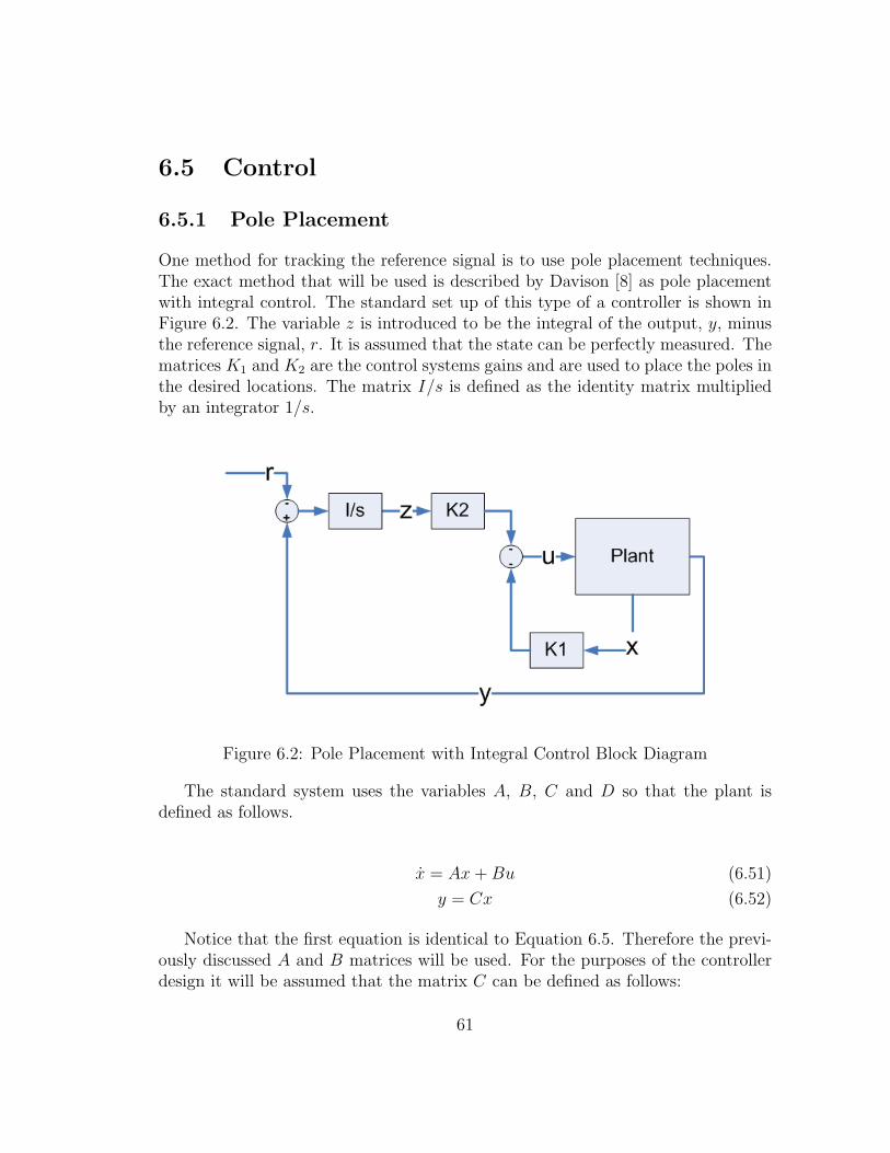
One method for tracking the reference signal is to use pole placement techniques.The exact method that will be used is described by Davison [8] as pole placementwith integral control. The standard set up of this type of a controller is shown inFigure 6.2. The variable z is introduced to be the integral of the output, y, minusthe reference signal, r. It is assumed that the state can be perfectly measured. Thematrices K1 and K2 are the control systems gains and are used to place the poles inthe desired locations. The matrix I/s is defined as the identity matrix multipliedby an integrator 1/s.

Figure 6.2: Pole Placement with Integral Control Block Diagram

The standard system uses the variables A, B, C and D so that the plant isdefined as follows.

x = Ax+Bu (6.51)

y = Cx (6.52)

Notice that the first equation is identical to Equation 6.5. Therefore the previ-ously discussed A and B matrices will be used. For the purposes of the controllerdesign it will be assumed that the matrix C can be defined as follows:

61

C =

[0 0 1 0 0 0 0 0 00 0 0 0 0 1 0 0 0

](6.53)

Using the above control structure an augmented state matrix set is constructedusing x, A, K,B and Br, which are defined and related as follows:

x = [x, z]T (6.54)

A =

[A 0C 0

](6.55)

B = [B, 0]T (6.56)

Br = [0,−I]T (6.57)

K = [K1, K2]T (6.58)

˙x = Ax+ Bu+ Brr (6.59)

Using this matrix structure, standard pole placement techniques (such as ’place’in the Matlab Control Systems Toolbox[32]) can be used to select the gain matrixK.

62

6.5.2 H-Infinity Control

One major problem with the pole placement technique is that it makes no guaranteeon disturbance rejection or robustness with respect to plant uncertainty. H∞ designis a technique that can account for disturbances and plant uncertainty. It willautomatically design controller that has a sensitivity function that falls within acertain specified bound. By using models for the disturbances, such as the windgust models previously discussed, and the plant uncertainty, that has hopefullybeen minimized using system identification techniques, a bound on the sensitivityfunction can be generated and used in the H∞ process.

Due to time limitations, this will not be discussed further and the reader willbe referred to a number of publications on the subject [12, 3].

63

6.5.3 Model Predictive Control

Another approach for the control of a parafoil system is model predictive control[36]. This was used by Slegers and Costello [39] to successfully control a smallparafoil and payload system to follow a specified track.

Model predictive control uses a dynamic model of the system to simulate forwarda certain number of time steps, known as the prediction horizon, and compares itspredicted state to its desired state. The controller can be designed to minimize thestate error and control signal energy throughout the prediction horizon.

Slegers [39] argued that model predictive control emulates the way humans thinkabout controlling a parachute. A skydiver looks at their current state and makesan educated guess about where they will be in the future and adjusts the controlsaccordingly.

There are a few drawbacks to the model predictive control method. Simulat-ing the future system output can be computationally expensive, especially if theprediction horizon is large. Additionally, the system can not account for resultsbeyond its prediction horizon and may not perform optimally if the horizon is toosmall. Lastly, this system can not easily account for uncertainties in the dynamicmodel and says nothing about the system’s disturbance rejection.

Despite these drawbacks, Slegers and Costello were able to land their parachutesystem within six feet of their desired target in crosswinds with speeds of twelvefeet per second. Their system used a linear model with four states for roll, yaw,roll rate and yaw rate. Their algorithm was updated once per second and has aprediction horizon of 10 seconds.

64

Chapter 7

Conclusions and FutureRecommendations

7.1 Conclusions

In conclusion, this report presented an overview of parachute flight, developed aset of equations for a six degree of freedom simulation and designed a guidance andcontrol system. From this report a number of conclusions can be made.

While investigating the basics of parachute flight, it was concluded that the ramair parafoil should be used as it provides the best glide slope ratio and the highestmaneuverability. The dynamics of deployment were investigated and a number ofrecommendations were made for the design of the deployment system. The mod-eling of the parachute system set up a framework for a non-linear simulation thatcan be used in future developments. During this investigation, it was hypothesizedthat a dynamic model that represents the parafoil and payload as separate bodieswill only be more accurate during transient behaviors.

The design of a guidance system concluded with a proposed algorithm thatwill track a path in the inertial frame by generating a desired glide slope ratioand track over ground that the control system must follow. The investigation of acontrol system presented the details of a method to design a controller using poleplacement methods. This included a method for linearizing the non-linear modelin such a way that it can track the commands given by the guidance system. Otheralternatives for a control system were briefly discussed. Specifically, H∞ controlwas proposed for its ability to optimize the trade off between model uncertaintyand disturbance rejection. Also, model predictive control was briefly discussed

65

because previous experimental studies have shown good results using this method.Additionally, suggestions for system identification and the design of a navigationsystem were outlined but the details of these were not presented.

7.2 Future Recommendations

A number of directions for future research are recommended by this report. Anoptimized parafoil and payload system should be designed and built. WARG cur-rently has a parachute system; however its performance needs to be improved.Additionally, a deployment system needs to be implemented. Using the knowledgeof some of the trade offs presented in this report; it should be possible to design asystem that meets the requirements.

Once a satisfactory parachute system is built, it is recommended that a systemidentification technique be used to identify the model parameters. With a relativelyaccurate model, the control system can be designed using the simplest technique,pole placement. If the pole placement technique does not give adequate tracking,the model predictive control technique should be implemented. If both of thesedo not give the necessary performance, the H∞ technique should be attempted.However, H∞ control will require further investigation into wind models and plantuncertainty and is not a simple design process.

It is also recommended that further investigation of the non-linear apparentmass terms be undertaken. Lastly, it is recommended that a visual navigationsystem be developed to make last minute corrections in the parachute’s trajectory.

66

Appendix A

Fourth Order Runge-KuttaMethod

The classic fourth order Runge-Kutta method (RK4) was used for solving the initialvalue problem in the simulator. The RK4 algorithm works by solving for the slopeat the current point, the end point and two mid-points. The first mid-point usesthe slope of the current point to calculate its y-location, while the second mid-pointuses the slope of the first mid-point to calculate its y-location. The end point usesthe second mid-point’s slope to calculate its y-location. A weighted average is usedto calculate the overall slope and the next y-location is found using this averagedslope [41]. The equations for a time invariant system are as follows. Note thatx = f(x, u), where x is the current state and u is the input. Also, dt is the timestep.

k1 = f(x, u) (A.1)

k2 = f(x+ 0.5k1, u) (A.2)

k3 = f(x+ 0.5k2, u) (A.3)

k4 = f(x+ 0.5k3, u) (A.4)

Now,

x = x+ dtk1 + 2k2 + 2k3 + k4

6(A.5)

The following matlab code was used to implement this algorithm.

67

0001 clear;

0002 T = 0.01;

0003 end time = 10;

0004 num of steps = floor(end time / T);

0005

0006 u=cell(1,num of steps);

0007 x=cell(1,num of steps);

0008

0009 x{1} = [0; 0; 0; 0; 0; 0; 7; 0; 2; 0; 0; 0];

0010

0011 for count = 1:num of steps

0012 u{count} = zeros(2,1);

0013 % if count * T > 14 && count * T < 14.5

0014 % u{count} = [0; 0.2];

0015 % end

0016

0017 % if count * T > 3 && count * T < 4

0018 % u{count} = [0.75; 0];

0019 % end

0020 end

0021

0022 disp = 0;

0023

0024 for step = 1:num of steps

0025 % x{step}(1:3)=[0;0;0];0026 x{step+1}=RK4 TI(@six dof parachute,T,x{step},u{step});0027 if disp == 100

0028 disp = 0;

0029 T*step

0030 else

0031 disp = disp + 1;

0032 end

0033 end

0034

0035 six dof plot(x,u,num of steps,T)

68

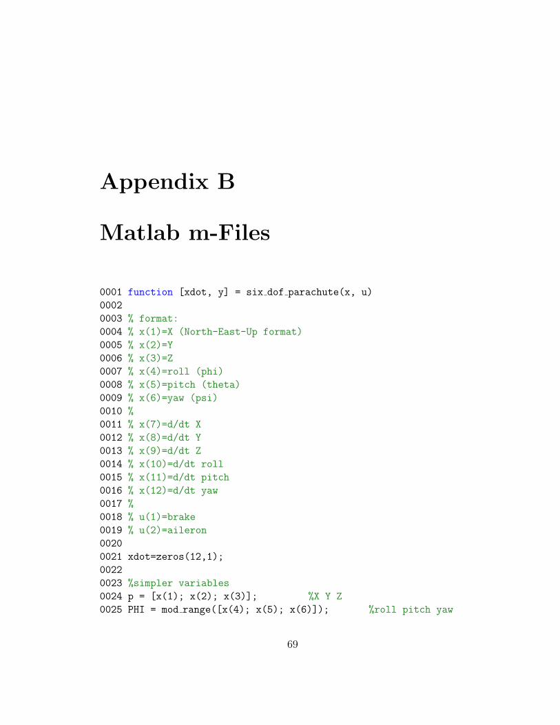
Appendix B

Matlab m-Files

0001 function [xdot, y] = six dof parachute(x, u)

0002

0003 % format:

0004 % x(1)=X (North-East-Up format)

0005 % x(2)=Y

0006 % x(3)=Z

0007 % x(4)=roll (phi)

0008 % x(5)=pitch (theta)

0009 % x(6)=yaw (psi)

0010 %

0011 % x(7)=d/dt X

0012 % x(8)=d/dt Y

0013 % x(9)=d/dt Z

0014 % x(10)=d/dt roll

0015 % x(11)=d/dt pitch

0016 % x(12)=d/dt yaw

0017 %

0018 % u(1)=brake

0019 % u(2)=aileron

0020

0021 xdot=zeros(12,1);

0022

0023 %simpler variables

0024 p = [x(1); x(2); x(3)]; %X Y Z

0025 PHI = mod range([x(4); x(5); x(6)]); %roll pitch yaw

69

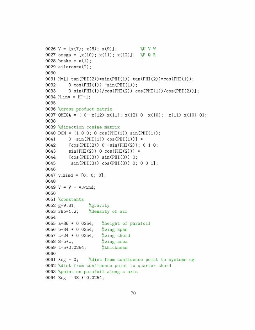
0026 V = [x(7); x(8); x(9)]; %U V W

0027 omega = [x(10); x(11); x(12)]; %P Q R

0028 brake = u(1);

0029 aileron=u(2);

0030

0031 H=[1 tan(PHI(2))*sin(PHI(1)) tan(PHI(2))*cos(PHI(1));

0032 0 cos(PHI(1)) -sin(PHI(1));

0033 0 sin(PHI(1))/cos(PHI(2)) cos(PHI(1))/cos(PHI(2))];

0034 H inv = H^-1;

0035

0036 %cross product matrix

0037 OMEGA = [ 0 -x(12) x(11); x(12) 0 -x(10); -x(11) x(10) 0];

0038

0039 %direction cosine matrix

0040 DCM = [1 0 0; 0 cos(PHI(1)) sin(PHI(1));

0041 0 -sin(PHI(1)) cos(PHI(1))] *

0042 [cos(PHI(2)) 0 -sin(PHI(2)); 0 1 0;

0043 sin(PHI(2)) 0 cos(PHI(2))] *

0044 [cos(PHI(3)) sin(PHI(3)) 0;

0045 -sin(PHI(3)) cos(PHI(3)) 0; 0 0 1];

0046

0047 v wind = [0; 0; 0];

0048

0049 V = V - v wind;

0050

0051 %constants

0052 g=9.81; %gravity

0053 rho=1.2; %density of air

0054

0055 a=36 * 0.0254; %height of parafoil

0056 b=84 * 0.0254; %wing span

0057 c=24 * 0.0254; %wing chord

0058 S=b*c; %wing area

0059 t=5*0.0254; %thickness

0060

0061 Xcg = 0; %dist from confluence point to systems cg

0062 %dist from confluence point to quarter chord

0063 %point on parafoil along z axis

0064 Zcg = 48 * 0.0254;

70

0065

0066 rigging angle = 10; %degrees

0067

0068 vc = sqrt(V’*V); %velocity

0069 qbar = 0.5 * rho * vc*vc; %dynamic pressure

0070 mass = 4; %mass in kg

0071 alpha = rad2deg(atan2(V(3), V(1))) - rigging angle;

0072

0073 %apparent mass terms

0074 A = 0.899 * pi() / 4 * t^2 * b;

0075 B = 0.39 * pi() / 4 * (t^2 + 2 * deg2rad(alpha)^2) * c;

0076 C = 0.783 * pi() / 4 * c^2 * b;

0077

0078 I A = 0.63 * pi() / 48 * c^2 * b^3;

0079 I B = 0.817 * 4 / (48*pi()) * c^4*b;

0080 I C = 1.001 * pi() / 48 * t^2 * b^3;

0081

0082

0083 K abc = [A 0 0; 0 B 0; 0 0 C];

0084 K Iabc = [I A 0 0; 0 I B 0; 0 0 I C];

0085

0086 [K abc; K Iabc];

0087

0088 % K abc = [0 0 0; 0 0 0; 0 0 0];

0089 % K Iabc = [0 0 0; 0 0 0; 0 0 0];

0090

0091 %inertia matrix

0092 J 1=1.3558*[.1357 0 .0025; 0 .1506 0; .0025 0 .0203];

0093

0094 %J 2= J 1+[I A 0 0; 0 I B 0; 0 0 I C];

0095 %J=J 2 + [0 0 Xcg*Zcg; 0 sqrt(Xcg*Xcg+Zcg*Zcg) 0;

0096 %Xcg*Zcg 0 0] * (mass+B);

0097 J = J 1 + mass * [Zcg^2 0 0; 0 Zcg^2 0; 0 0 0];

0098

0099 %Aerodynamic Coefficients - Iacomini & Cerimele

0100 CL o=0.2;

0101 CL alpha=0.0375;

0102 CL brake=0.377;

0103

71

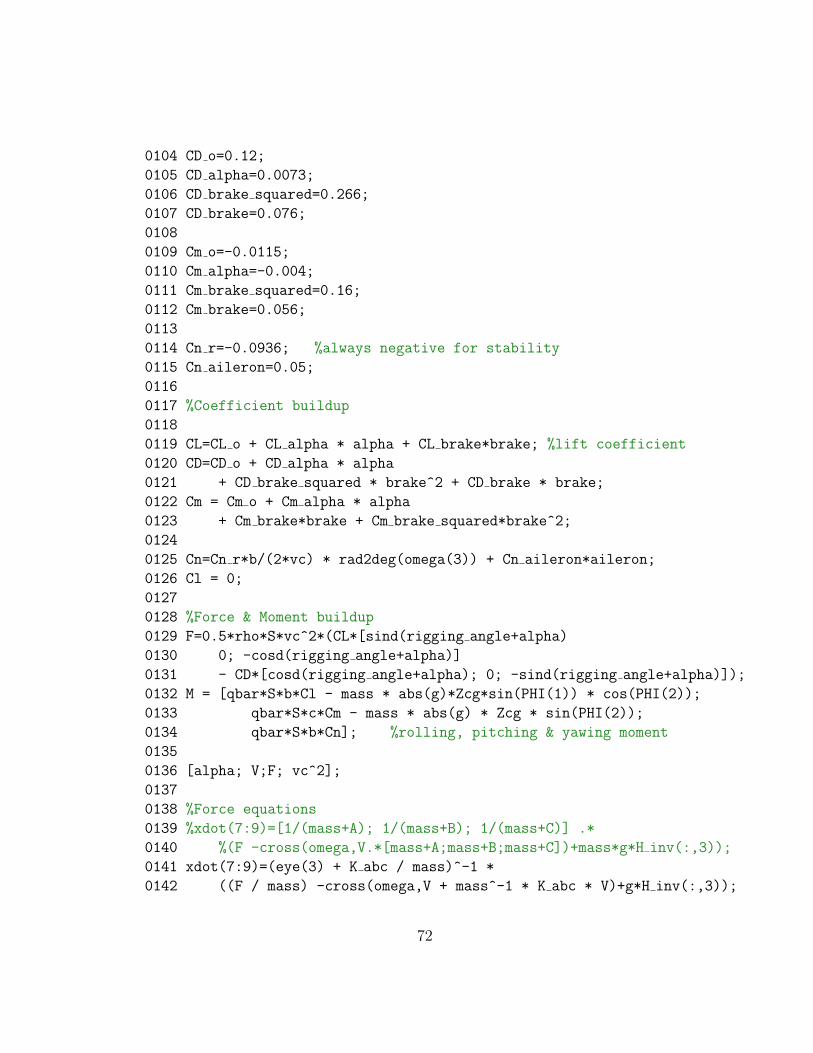
0104 CD o=0.12;

0105 CD alpha=0.0073;

0106 CD brake squared=0.266;

0107 CD brake=0.076;

0108

0109 Cm o=-0.0115;

0110 Cm alpha=-0.004;

0111 Cm brake squared=0.16;

0112 Cm brake=0.056;

0113

0114 Cn r=-0.0936; %always negative for stability

0115 Cn aileron=0.05;

0116

0117 %Coefficient buildup

0118

0119 CL=CL o + CL alpha * alpha + CL brake*brake; %lift coefficient

0120 CD=CD o + CD alpha * alpha

0121 + CD brake squared * brake^2 + CD brake * brake;

0122 Cm = Cm o + Cm alpha * alpha

0123 + Cm brake*brake + Cm brake squared*brake^2;

0124

0125 Cn=Cn r*b/(2*vc) * rad2deg(omega(3)) + Cn aileron*aileron;

0126 Cl = 0;

0127

0128 %Force & Moment buildup

0129 F=0.5*rho*S*vc^2*(CL*[sind(rigging angle+alpha)

0130 0; -cosd(rigging angle+alpha)]

0131 - CD*[cosd(rigging angle+alpha); 0; -sind(rigging angle+alpha)]);

0132 M = [qbar*S*b*Cl - mass * abs(g)*Zcg*sin(PHI(1)) * cos(PHI(2));

0133 qbar*S*c*Cm - mass * abs(g) * Zcg * sin(PHI(2));

0134 qbar*S*b*Cn]; %rolling, pitching & yawing moment

0135

0136 [alpha; V;F; vc^2];

0137

0138 %Force equations

0139 %xdot(7:9)=[1/(mass+A); 1/(mass+B); 1/(mass+C)] .*

0140 %(F -cross(omega,V.*[mass+A;mass+B;mass+C])+mass*g*H inv(:,3));

0141 xdot(7:9)=(eye(3) + K abc / mass)^-1 *

0142 ((F / mass) -cross(omega,V + mass^-1 * K abc * V)+g*H inv(:,3));

72

0143 % [(eye(3) + K abc / mass); alpha V(3) V(1)]

0144

0145 %Kinematic Equations

0146 xdot(4:6)= H * omega;

0147

0148 %Moment Equations

0149 % xdot(10:12)=(J^-1) * (M - OMEGA * J * ([I A; I B; I C]

0150 %.* omega)+cross(V,V.*[mass+A;mass+B;mass+C]));

0151 % xdot(10:12)=(J + K Iabc)^-1 * (M - OMEGA * J * omega);

0152 xdot(10:12)=(J + K Iabc)^-1 *

0153 (M -cross(omega,K Iabc * omega) -

0154 cross(V,K abc * V) - OMEGA * J * omega);

0155

0156

0157 %Navigation Equations

0158 xdot(1:3) = [1 0 0; 0 1 0; 0 0 -1] * DCM’ * V;

73

Bibliography

[1] Nasa dryden fact sheets - x-38. http://www.nasa.gov/centers/dryden/

news/FactSheets/FS-038-DFRC.html, May 2006.

[2] J. D. Anderson. Introduction to Flight. McGraw Hill, 2004.

[3] J. W. Helton B. Francis and G. Zames. h∞ optimal feedback controllers forlinear multivariable systems. Technical Report 10, IEEE Transactions on Au-tomatic Controls, October 1984.

[4] W. L. Brogan. Modern Control Theory. Prentice Hall, 3 edition, 1991.

[5] G. J. Brown. Parafoil steady turn response to control input. Technical Report93-1241, American Institute of Aeronautics and Astronautics, 1993.

[6] FAI International Parachute Commission. Competition rules for freefall styleand accurracy. ftp://www.fai.org/parachuting/competition_rules/sa_

2006.pdf, March 2006.

[7] D. Davison. Course notes: Digital control applications, ece 484, Jan 2006.

[8] D. Davison. Course notes: Multivariable control systems, ece 488, May 2006.

[9] R. C. Dorf and R. H. Bishop. Modern Control Systems. Pearson Prentice Hall,10 edition, 2005.

[10] A. A. Proctor et al. Ongoing development of an autonomous aerial recon-naissance system at georgia tech. Technical report, Journal of the AUVSIUnmanned Systems Symposium Proceedings, 2004.

[11] B. E. Tweddle et al. A network-based implementation of an aerial robotic sys-tem. Technical report, Journal of the AUVSI Unmanned Systems SymposiumProceedings, 2004.

74

[12] J. C. Doyle et al. State-space solutions of standard h2 and h∞ control problems.Technical Report 8, IEEE Transactions on Automatic Controls, August 1989.

[13] P. A. Mortaloni et al. On the development of a six-degree-of-freedom modelof a low-aspect-ratio parafoil delivery system. Technical Report 2003-2105,American Institute of Aeronautics and Astronautics, May 2003.

[14] T. A. Bonneau et al. Implementation of an autonomous multivehicle system.Technical report, Journal of the AUVSI Unmanned Systems Symposium Pro-ceedings, 2000.

[15] T. A. Bonneau et al. Southern polytechnic state university autonomous remotereconnaissance system. Technical report, Journal of the AUVSI UnmannedSystems Symposium Proceedings, 2004.

[16] B. Etkin. Dynamics of Flight: Stability and Control. John Wiley and Sns, 2edition, 1982.

[17] J. D. Powell F. F. Franklin and M. Workman. Digital Control of DynamicSystems. Addison Wesley Longman, Inc., 3 edition, 1998.

[18] J. H. Ginsberg. Advanced Engineering Dynamics. Cambridge University Press,2 edition, 1998.

[19] P. D. Hattis and R. Benney. Demonstration of precision-guided ram-air parafoilairdrop using gps/ins navigation. Technical report, Proceedings of the Instituteof Navigation’s 52nd Annual General Meeting, June 1996.

[20] E. J. Haug. Computer-Aided Kinematics and Dynamics of Mechanical Systems,volume 1. Allyn and Bacon, 1989.

[21] C. S. Iacomini and C. J. Cerimele. Lateral-directional aerodynamics from alarge scale parafoil test program. Technical Report 99-1731, American Instituteof Aeronautics and Astronautics, 1999.

[22] C. S. Iacomini and C. J. Cerimele. Longitudinal aerodynamics from a largescale parafoil test program. Technical Report 99-1732, American Institute ofAeronautics and Astronautics, 1999.

[23] C. S. Iacomini and C. M. Madsen. Investigation of large scale parafoil riggingangles: Analytical and drop test results. Technical Report 99-1752, AmericanInstitute of Aeronautics and Astronautics, 1999.

75

[24] Mist Mobility Integrated Systems Technology Inc. Mmist sherpa. http://

www.mmist.ca/Sherpa.asp, May 2006.

[25] D. C. Jalbert. Multi-cell wing type aerial device, November 1966.

[26] T. Jann. Aerodynamic model identification and gnc design for the parafoil-loadsystem alex. Technical Report 93-1241, American Institute of Aeronautics andAstronautics, 1993.

[27] J. Dooley K. Brock and F. Manning. Development of an autonomous aerialreconnaissance system. Technical report, Journal of the AUVSI UnmannedSystems Symposium Proceedings, 2004.

[28] T. W. Knacke. Parachute Recovery Systems Design Manual. Para Publishing,1992.

[29] J. S. Lingard. The aerodynamics of gliding parachutes. Technical ReportPR-409, Martin-Baker Aircraft Co. Ltd., 1990.

[30] P. B. S. Lissaman and G. J. Brown. Apparent mass effects on parafoil dy-namics. Technical Report 93-1236, American Institute of Aeronautics andAstronautics, 1993.

[31] United States Marines. Image:usmc paratrooper.jpg. http://en.wikipedia.org/wiki/Image:USMC_Paratrooper.jpg. Accessed August 28, 2006.

[32] The MathWorks. Matlab, 2006.

[33] R. Michelson. Rules for the current international aerial robotics com-petition mission. http://avdil.gtri.gatech.edu/AUVS/CurrentIARC/

200xCollegiateRules.html, May 2006.

[34] U.S. Department of Defense Handbook. Mil-hdbk-1797: Flying qualities ofpiloted vehicles, 1997.

[35] D. Poynter. The Parachute Manual, volume 2. Para Publishing, 1991.

[36] J. B. Rawlings. Tutorial overview of model predictive control. Technical Re-port 3, IEEE Control Systems Magazine, June 2000.

[37] R. M. Rogers. Aerodynamic parameter estimation for controlled parachutes.Technical Report 2002-4708, American Institute of Aeronautics and Astronau-tics, August 2002.

76

[38] V. Saalo. Image:flight dynamics.jpg. http://en.wikipedia.org/wiki/

Image:Flight_dynamics.jpg. Accessed August 28, 2006.

[39] N. Slegers and M. Costelllo. Model predictive control of a parafoil and pay-load system. American Institute of Aeronautics and Astronautics Journal ofGuidance, Control and Dynamics, 28(4):816–821, 2005.

[40] N. Slegers and M. Costello. Aspects of control for a parafoil and payloadsystem. AIAA Journal of Guidance, Control and Dynamics, 26(6):898–905,2003.

[41] B.L. Stevens and F. L. Lewis. Aircraft Control and Simulation. John Wileyand Sons, Inc., 2 edition, 2003.

[42] B. E. Tweddle. Integration of an attitude heading reference system with theglobal positioning system. Technical Report WTR 400, University of Waterloo,Department of Electrical and Computer Engineering, May 2006.

[43] Unknown. Image:ram air square.jpg. http://en.wikipedia.org/wiki/

Image:Ram_air_square.jpg. Accessed August 28, 2006.

77

Simulation and Control of Guided Ram Air Parafoils · PDF file29.08.2006 ·...

Documents

Transcript of Simulation and Control of Guided Ram Air Parafoils · PDF file29.08.2006 ·...