
Simulating the Greeks in Finance - Columbia University · Simulating the Greeks in Finance By: ......
21
✬ ✫ ✩ ✪ Simulating the Greeks in Finance By: John Lehoczky Carnegie Mellon University June 7, 2012 John Lehoczky 1
-
Upload
nguyentruc -
Category
Documents
-
view
219 -
download
0
Transcript of Simulating the Greeks in Finance - Columbia University · Simulating the Greeks in Finance By: ......

'
&
$
%
Simulating the Greeks in Finance
By:
John LehoczkyCarnegie Mellon University
June 7, 2012 John Lehoczky 1

'
&
$
%
Outline
• Background on Greeks, problems with barrier options
• Representation of Greeks as an expected value
• Capriotti’s method for determining a good importance samplingdistribution
• Combining variance reduction methods for a specific problem
June 7, 2012 John Lehoczky 2
'
&
$
%
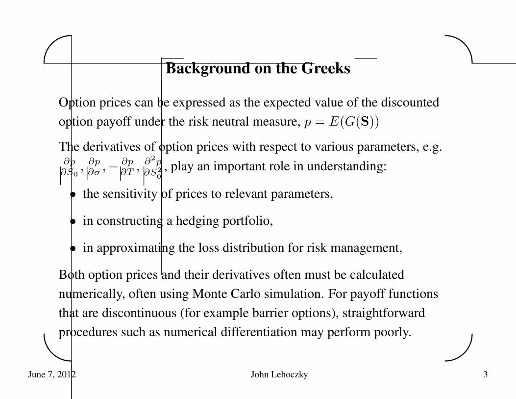
Background on the Greeks
Option prices can be expressed as the expected value of the discountedoption payoff under the risk neutral measure, p = E(G(S))
The derivatives of option prices with respect to various parameters, e.g.∂p∂S0
, ∂p∂σ
,− ∂p∂T
, ∂2p
∂S2
0
, play an important role in understanding:
• the sensitivity of prices to relevant parameters,
• in constructing a hedging portfolio,
• in approximating the loss distribution for risk management,
Both option prices and their derivatives often must be calculatednumerically, often using Monte Carlo simulation. For payoff functionsthat are discontinuous (for example barrier options), straightforwardprocedures such as numerical differentiation may perform poorly.
June 7, 2012 John Lehoczky 3

'
&
$
%
Example: Knock-in Digital Option
Consider an example (4.6.4, p264-267 in Glasserman’s text):
{St, t ≥ 0} is a GBM with parameters µ, σ, so
dSt = rStdt + σdWt,
under the risk neutral measure.
A continuous European knock-in digital option has a payoff functiongiven by
G(S) = ce−rT I{min0≤t≤T St} · I{ST≥K}.
The discrete version would replace the event {min0≤t≤T St ≤ H} with{min0≤i≤N Sih ≤ H}.
The prices and Greeks are different but will converge as N increases.
June 7, 2012 John Lehoczky 4

'
&
$
%
Estimating Delta for the Knock-in Digital Option
The most obvious way to estimate a derivative is to set up a numericaldifference quotient, e.g.
δ̂ ≈p̂(S0 + h) − p̂(S0 − h)
2h
= (
n∑
i=1
I(x + h) −
n∑
i=1
I(x − h))/2nh
= (n
∑
i=1
(I(x + h) − I(x − h)))/2nh
The summands will be 0, +1 or -1, and the probability of ±1 is O(h ∗ δ).
The estimate is biased and the variance is O((nh)−1). Consequently, avery large sample size is needed to overcome the h in the denominator.
June 7, 2012 John Lehoczky 5

'
&
$
%
Numerical derivatives for the Glasserman Example
Consider 1,000,000 paths for S0 = 95, H = 90, K = 96
• 619,351 did not reach H
• 337,826 reached H but not K
• 42,819 both x-h and x+h paid off, but they cancelled each other
• 4 made a contribution to the numerator
June 7, 2012 John Lehoczky 6

'
&
$
%
Representing the Greeks as an Expected ValueIn 1996, Broadie and Glasserman developed two methods to representGreeks as expected values as opposed to numerical derivatives: pathwiseand log-likelihood derivatives. For S0 = x and s = (s1, . . . , sN ),price(x) = p(x) =
∫
. . .∫
G(s)f(s|x)ds.
∂p(x)
∂x=
∂
∂x
∫
. . .
∫
G(s)f(s|x)ds
=
∫
. . .
∫
∂
∂xG(s)f(s|x)ds
=
∫
. . .
∫
G(s)∂
∂xf(s|x)ds
=
∫
. . .
∫
G(s)(∂
∂xlog f(s|x))f(s|x)ds
= E(G(S)∂
∂xlog f(S|x)).
June 7, 2012 John Lehoczky 7

'
&
$
%
Formalization Using Malliavin Calculus
The two methods of Broadie and Glasserman express the Greeks (delta inthe case at hand) as an expectation which can be unbiasedly estimated byMonte Carlo simulation.
The log-likelihood approach required determination of ∂∂x
log f(S|x),which is easy for GBM, but requires an Euler discretization in general, forwhich the transitions are conditionally normal.
A general method was developed by Fournie, Lasry, Lebuchoux, Lionsand (Touzi) in 1999 and 2001 based on an integration by parts formulafrom the Malliavin Calculus.
June 7, 2012 John Lehoczky 8

'
&
$
%
Fournie et al Results for DeltaAssume
dXt = b(X(t))dt + σ(X(t))dW (t),
and the discounted payoff, G, is determined by a set of times0 ≤ t1 < . . . < tN = T , so
p(x) = E(G(Xt1 , . . . , XtN)|X0 = x).
Yt, t ≥ 0, Y (t) = dXt/dx is the first variation process or pathwisederivative satisfies.
dYt = b′(Xt)Ytdt + σ′
(Xt)YtdWt,
then (FLLLT I, Proposition 3.2, p399)
p′
(x) = E(G(Xt1 , . . . , XtN)1
T
∫ T
0
Yt
σ(Xt)dWt).
June 7, 2012 John Lehoczky 9

'
&
$
%
Malliavin-Based Greeks
The expression for δ and other Greeks does not require knowledge of thelikelihood function as required by the Broadie and Glasserman approach.In general, one needs to discretize X and Y .
In 2007, Chen and Glasserman began with the likelihood approach andintroduced an Euler discretization for the underlying X process. Thetransition densities are conditionally normal, and the log-likelihood iseasily written.
They showed that as the time increments converge to 0, thelog-likelihood-based estimates converge to the Malliavin calculus-basedestimates, so either approach can be used.
June 7, 2012 John Lehoczky 10

'
&
$
%
Partial List of work on the Greeks
• Broadie and Glasserman, 1996 “Estimating security price derivativesusing simulation,” Management Science.
• Fournie, Lasry, Lebuchoux, Lions and Touzi, 1999, “Applications ofMalliavin calculus to Monte Carlo Method in Finance, I” Financeand stochastics.
• Fournie, Lasry, Lebuchoux, and Lions, 2001, “Applications ofMalliavin calculus to Monte Carlo Method in Finance, II” Financeand Stochastics
• Benhamou 2003 “Optimal Malliavin weighting function for thecomputation of Greeks,” Mathematical Finance
June 7, 2012 John Lehoczky 11

'
&
$
%
Partial List of Work on the Greeks
• Gobet and Kohatsu-Higa, 2003 “Computation of Greeks for barrierand lookback options using Malliavin calculus” ElectronicCommunications in Probability.
• Cvitanic, Ma and Zhang, 2003 “Efficient computation of hedgingportfolios for options with discontinuous payoffs,” MathematicalFinance.
• Davis and Johansson, 2006 “Malliavin Monte Carlo Greeks for jumpdiffusions,” Stochastic Processes and their Applications.x
• Chen and Glasserman, 2007 “Malliavin Greeks without Malliavincalculus”, Stochastic Processes and Their Application.
June 7, 2012 John Lehoczky 12

'
&
$
%
The Knock-in Barrier Option Issues: 1
In considering Glasserman’s example, there are a number of issues andapproaches that arise:
• Numerical derivatives will be biased and require huge sample sizesfor sufficient accuracy.
• The Likelihood method or the Malliavin derivative approach willrecast the Greek to be an expected value, i.e.δ = E(G(S) · weight function)
• The likelihood method is still vulnerable to failure of the knock-incondition to be satisfied, especially if S0, K, and H are somewhat farapart. This problem can be solved by importance sampling. Willdiscuss Capriotti’s method to determine an optimal importancesampling distribution.
June 7, 2012 John Lehoczky 13

'
&
$
%
The Knock-in Barrier Option Issues: 2
• The variance can be further reduced by combining conditional MonteCarlo methods. For delta under GBM, once the knock-in condition issatisfied, if ever, the price of the Greek can be determinedanalytically. Using this can reduce the variance significantly.
• Extensions to other Greeks and to more general price processespossibly using Euler discretization.
June 7, 2012 John Lehoczky 14

'
&
$
%
Importance Sampling: Capriotti’s Method 1
In 2008, L. Capriotti (Quantitative Finance, 8, 485-497) developed amethod to find a good importance sampling distribution based on anon-linear least squares approach.
Suppose P0 corresponds to the risk-neutral measure, and suppose there isa family of possible importance sampling distributions indexed by θ,{Pθ, θ ∈ Θ}. The goal is to find θ to minimize the variance of theimportance sampled estimator.
For example, Θ = {θ = (µ, η); µ ∈ (−∞,∞), η > 0} corresponding tochanges from N(0, 1) to N(µ, η2).
The above example assumes that all random variables used to construct apath have the same distribution. But this can be generalized to allowdifferent changes for different parts of the path; for example allowing themean to vary with time to price an Asian option.
June 7, 2012 John Lehoczky 15

'
&
$
%
Importance Sampling: Capriotti’s Method 2
A preliminary simulation-based non-linear least squares analysis isconducted to determine a good θ using a sample of size M . This isfollowed by a relatively large study with sample size n >> M usingimportance sampling to reach the desired low-variance estimate.
LetWθ =
dP0
dPθ
, ∀θ ∈ Θ.
NoteE0(G(S)) = Eθ(G(S)Wθ(S)), θ ∈ Θ
where G is the discounted payoff function.
June 7, 2012 John Lehoczky 16
'
&
$
%
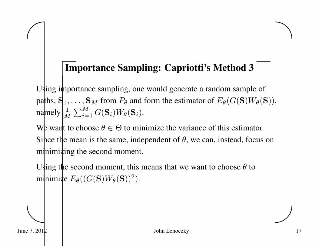
Importance Sampling: Capriotti’s Method 3
Using importance sampling, one would generate a random sample ofpaths, S1, . . . ,SM from Pθ and form the estimator of Eθ(G(S)Wθ(S)),namely 1
M
∑M
i=1G(Si)Wθ(Si).
We want to choose θ ∈ Θ to minimize the variance of this estimator.Since the mean is the same, independent of θ, we can, instead, focus onminimizing the second moment.
Using the second moment, this means that we want to choose θ tominimize Eθ((G(S)Wθ(S))2).
June 7, 2012 John Lehoczky 17

'
&
$
%
Importance Sampling: Capriotti’s Method 4
Eθ((G(S)Wθ(S))2) =
∫
(G(S)Wθ(S))2dPθ(S)
=
∫
G2(S)Wθ(S)Wθ(S)dPθ(S)
=
∫
G2(S)Wθ(S)dP0(S)
= E0(G2(S)Wθ(S)).
It follows that we want to minimize the final quantity, E0(G2(S)Wθ(S)),
where the random paths, S, now come from the original probabilitydistribution, P0.
June 7, 2012 John Lehoczky 18

'
&
$
%
Importance Sampling: Capriotti’s Method 5
Now, E0(G2(S)Wθ(S)) can be estimated from the paths S1, . . . ,SM by
1
M
∑M
i=1G2(Si)Wθ(Si). Ignoring the constant 1
M, we want to minimize
∑M
i=1G2(Si)Wθ(Si).
To solve this optimization problem, consider the statistical model
Y = G(X)√
Wθ(X) + ε.
This is a non-linear model. Suppose we have values X1, . . . ,XM , and weuse those values to create model data given by{(G(Xi)
√
Wθ(Xi), 0), 1 ≤ i ≤ M} (so the dependent variable valuesare all 0.
June 7, 2012 John Lehoczky 19

'
&
$
%
Importance Sampling: Capriotti’s Method 6
The least squares solution given these data will find the θ that minimizesthe squared residuals, i.e.
∑M
i=1(Yi − G(Xi)
√
Wθ(Xi))2.
However, since Yi = 0, this minimizes∑M
i=1G2(Xi)Wθ(Xi), the second
moment expression we sought to minimize.
Thus, approximating the optimal importance sampling distribution isequivalent to finding the non-linear least squares estimator in the abovestatistical model with Y = 0. The resulting θ̂ is approximately optimal,since it is, in fact, a random variable derived from the initial X data.
Capriotti suggest using the Levenberg-Marquandt non-linear least squaresalgorithm. This is implemented in Matlab by nlinfit.
June 7, 2012 John Lehoczky 20

'
&
$
%
Results for Glasserman Example: Delta
For T = .25, N = 50, r = .05, σ = .15, S0 = 95 and payoff = $10,000,Pθ = N(θ, 1).
H K Delta Var Ratio 1 Var Ratio 2 θ
94 96 -544.7 2.62 3.32 -.2490 96 -136.68 6.65 22.21 -.3685 96 -2.86 52.71 1714 -.5690 106 -6.51 120.64 774.9 -.52
Var Ratio 1 = Standard MC versus Conditional MCVar Ratio 2 = Standard MC versus Cond. MC and Imp. Sampling
June 7, 2012 John Lehoczky 21