Simulating Solitons of the Sine-GordonEquation using Variational Approximations

and Hamiltonian Principles

ByEvan Foley

A SENIOR RESEARCH PAPER PRESENTED TO THE DEPARTMENT OF MATHEMATICSAND COMPUTER SCIENCE OF STETSON UNIVERSITY IN PARTIAL FULFILLMENT OF

THE REQUIREMENTS FOR THE DEGREE OF BACHELOR OF SCIENCE

STETSON UNIVERSITY

1

Acknowledgements

I would like to thank Dr. Vogel for his patience, cooperation, and guidance with the research.

I would like to thank the Stetson Undergraduate Research Experience (SURE) program for

providing me the opportunity to work with Dr. Vogel in an one on one environment over the

summer of 2012.

2

Contents

Acknowledgements . . . . . . . . . . . . . . . . . . . . . . . . . . . . . . . . . . . . . . . . 2

List of Figures . . . . . . . . . . . . . . . . . . . . . . . . . . . . . . . . . . . . . . . . . . 4

Abstract . . . . . . . . . . . . . . . . . . . . . . . . . . . . . . . . . . . . . . . . . . . . . . 5

1 Introduction 6

2 Approximation Method on Korteweg-de Vries Equations 7

2.1 Elementary . . . . . . . . . . . . . . . . . . . . . . . . . . . . . . . . . . . . . . . . . 7

2.2 Modified . . . . . . . . . . . . . . . . . . . . . . . . . . . . . . . . . . . . . . . . . . . 10

3 Approximation Method on the Sine-Gordon Equation 12

3.1 Gaussian Wave Trial Function . . . . . . . . . . . . . . . . . . . . . . . . . . . . . . . 12

3.1.1 Traveling Wave Solution . . . . . . . . . . . . . . . . . . . . . . . . . . . . . . 12

3.1.2 Dynamic Solution . . . . . . . . . . . . . . . . . . . . . . . . . . . . . . . . . 13

3.2 Odd Oriented Gaussian Wave Trial Function . . . . . . . . . . . . . . . . . . . . . . 19

3.2.1 Traveling Wave Solution . . . . . . . . . . . . . . . . . . . . . . . . . . . . . . 19

3.2.2 Dynamic Solution . . . . . . . . . . . . . . . . . . . . . . . . . . . . . . . . . 20

4 Conclusions/Future Research 26

5 Appendices 27

5.1 Mathematica Code . . . . . . . . . . . . . . . . . . . . . . . . . . . . . . . . . . . . . 27

References 28

3

List of Figures

1 Original KdV: Amplitude and width vs. speed. . . . . . . . . . . . . . . . . . . . . . 9

2 Original KdV: Approximate and exact amplitude(left)/width(right) vs. speed. . . . 9

3 Modified KdV: Amplitude and speed vs. width. . . . . . . . . . . . . . . . . . . . . . 11

4 Modified KdV: Approximate and exact amplitude(left)/width(right) vs. speed. . . . 11

5 G Trial TWS Sine-Gordon: Amplitude and width paired with speed. . . . . . . . . . 13

6 G Trial DWS Sine-Gordon: Amplitude and width as functions of time. . . . . . . . . 17

7 G Trial DWS Sine-Gordon: Wave at times t=0,1,2,3,4 respectively (left to right, top

to bottom) . . . . . . . . . . . . . . . . . . . . . . . . . . . . . . . . . . . . . . . . . 18

8 OOG Trial TWS Sine-Gordon: Amplitude and width paired with speed. . . . . . . . 20

9 OOG Trial DWS Sine-Gordon: Amplitude, width, and center line position as func-

tions of time . . . . . . . . . . . . . . . . . . . . . . . . . . . . . . . . . . . . . . . . 25

10 G Trial DWS Sine-Gordon: Wave at times t=0,0.04,0.08 respectively (left to right,

top to bottom). . . . . . . . . . . . . . . . . . . . . . . . . . . . . . . . . . . . . . . . 26

4

Abstract

Simulating Solitons of the Sine-Gordon Equation using Variational Approximations andHamiltonian Principles

ByEvan FoleyMay 2013

Advisor: Dr. Thomas VogelDepartment: Mathematics and Computer Science

This project examines the underlying principle of soliton solutions in partial differential equa-

tions using Hamilton’s Principal and Variational Approximations. William Hamilton formulated

the idea that physical models can be described in terms of energies instead of the Newtonian pos-

turing in terms of forces. Using the concept of functionals, we can describe these energies in the

form of what is known as the Lagrangian to facilitate finding approximate solutions. Equations

such as the Korteweg-de Vries (KdV), Modified KdV, and the Sine-Gordon will be examined to

find localized structure (i.e. soliton) solutions. Interestingly enough, solitons behave differently

than typical waves, due to their unique characteristics which will be addressed throughout this

work. The solutions to these equations shall yield two results, justify the existence of solitons in

the governing equation and provide an approximate geometric structure for the solutions to the

PDEs that are under consideration.

5

1 Introduction

In 1834, a Scottish naval engineer, named John Scott Russell, was conducting an experiment at

the Union Canal in Scotland. He tried to establish a conversion factor between steampower and

horsepower by tying two horses on opposite sides of the canal to a steamboat, while he observed

on a horse on one side. While the horses were pulling the stationary steamboat, the ropes snapped

and something unexpected happened. The boat was shaken around and a wave popped out in

front of the boat, but the wave was not an ordinary wave. Russell described the wave as ”a

rounded, smooth, and well-defined heap of water.” He followed it for a couple of miles until the

canal prevented him from moving onward. Russell tried to recreate the wave that he saw but had

not been successful. Around that time, Newton and Bernoulli had formulated linear equations for

explaining hydrodynamics, so Russell’s observation was rejected from physicists. By 1895, Diederik

Korteweg and Gustav de Vries had derived a non-linear, partial differential equation, called the

KdV equation, that would model the behavior of what will be known as a soliton wave observed

by John Scott Russell [1].

A soliton can simply be described as a solitary wave with a localized structure that does not

diminish over time. The soliton wave is also known as the ’Wave of Translation’. A soliton wave is

said to have four distinct properties:

1. Stable and travels over long distances.

2. Speed depends on height and width of wave on the depth of water.

3. Multiple waves never merge, rather, they pass through each other.

4. If the wave is too big for depth of water, it will split into two.

William Hamilton developed the concept of energies describing physical systems and formalized

Hamilton’s Principle. Hamilton’s Principle can be summarized as follows: Of all possible paths

along which a dynamical system may evolve within a specified time interval, the actual path followed

is that which minimizes the time integral of the difference between the kinetic and potential energies

which is called the action, S.

S =

∫ t2

t1

(T − U)dt (1)

6

where

L = T − U (2)

where L=f[x,y(x),y’(x)] and is called the Lagrangian. In our case, we will integrate the action over

R in the spatial domain.

To minimize the action, we use the formula:

δS

δy= Sy −

d

dxSy′ = 0 (3)

where y is a parameter of the action [1]. One thing to note is that the action is not considered

a function, but a functional. In Variational Calculus, a functional is an operator that outputs

numbers where the input is a function. For instance, a definite integral is considered a functional.

Keeping the action in mind, there is a necessary condition that the lagrangian must satisfy called

the Euler-Lagrange equation [2, p. 125]:

Ly −d

dxLy′ = 0 (4)

where y=f(x). By applying the correct Lagrangian to this condition, the original partial differential

equation should arise.

2 Approximation Method on Korteweg-de Vries Equations

2.1 Elementary

The first equation that will be analyzed is the Korteweg-de Vries (KdV) Equation which is as

follows [3]:

ut + uux + uxxx = 0 (5)

This equation was originally designed to model the motion of a wave in shallow water.

To start off, assume the soliton is a traveling wave solution, meaning the only parameter chang-

7

ing with respect with to time is it’s position which can be described as

ξ = x− ct (6)

To start the approximation, the trial function needs to be defined. Based on the geometry of a

soliton wave, the Gaussian wave will be used as the trial function:

u(ξ) = Ae− ξ2

ρ2 (7)

Applying the necessary condition (4), the following Lagrangian can be found:

L = −1

2cu2 +

1

6u3 − 1

2(u′)2 (8)

The resulting action is:

S =A2√π(2

√3Aρ2 − 9

√2(cρ2 + 1))

36ρ(9)

When minimizing the action, two Euler Lagrange equations arise since there are two parameters

that we are interested in.

∂S

∂ρ=

A2√π(2√3Aρ2 − 9

√2(cρ2 − 1))

36ρ2= 0 (10)

∂S

∂A=

A√π(√3Aρ2 − 3

√2(cρ2 + 1))

6ρ= 0 (11)

Figure 1 shows the amplitude (red) and speed (blue) of the wave vary with respect to the wave

width.

8

0 1 2 3 4 5

20

40

60

80

100

Figure 1: Original KdV: Amplitude and width vs. speed.

Since the exact solution for the KdV equation is known, namely

u(ξ) = 3c sech2(

√cξ

2) (12)

the approximations (blue) can be compared to the exact (red) solution in Figure 2.

100 200 300 400 500

200

400

600

800

1000

1200

1400

0 10 20 30 40 50

1

2

3

4

5

Figure 2: Original KdV: Approximate and exact amplitude(left)/width(right) vs. speed.

Looking at the graphs, the solutions obtained from the approximation method very closely

resemble the exact solutions, this shows how accurate the method is.

9

2.2 Modified

Aside from the regular KdV equation, many modified versions have been created and tested, how-

ever, this research will only examine one [3]:

ut + 6u2ux + uxxx = 0 (13)

There will still be an assumption that the soliton is in a stationary state from earlier, with the

same trial function:

u(ξ) = Ae− ξ2

ρ2 (14)

Apply the necessary condition (4) and the following Lagrangian is obtained

L = −1

2cu2 +

1

2u4 − 1

2(u′)2 (15)

The action becomes

S =A2√π(A2ρ2 −

√2(cρ2 + 1))

4ρ(16)

The two Euler Lagrange equations that spawn from minimizing the action are:

∂S

∂ρ=

A2√π(A2ρ2 +√2(1− cρ2))

4ρ2= 0 (17)

∂S

∂A=

A√π(2A2ρ2 −

√2(cρ2 + 1))

2ρ= 0 (18)

Figure 3 displays Amplitude (red) and speed (blue) vs. width of the soliton wave.

10

0 1 2 3 4 5

20

40

60

80

100

Figure 3: Modified KdV: Amplitude and speed vs. width.

Since the exact solution to this Modified KdV Equation is known, namely

u(ξ) =√c sech

√cξ (19)

then a comparison is in order to determine how accurate the approximations (blue) are compared

to exact (red), shown in Figure 4.

100 200 300 400 500

5

10

15

20

0 10 20 30 40 50

1

2

3

4

5

Figure 4: Modified KdV: Approximate and exact amplitude(left)/width(right) vs. speed.

Based on the graphs, the method is producing very accurate results.

11

3 Approximation Method on the Sine-Gordon Equation

Now that the method is known to produce reasonable results, it is time to finally test the method

on the Sine-Gordon equation. We will use different trial functions to find different sets of solutions.

The Sine Gordon equation is [4]

utt − uxx + sinu = 0 (20)

The Sine-Gordon equation was founded in the 19th century and became quite popular once soli-

ton solutions were discovered. Some applications of the Sine-Gordon equation include: negative

Gaussian curvature, relativistic field theory, and dislocation in crystals. [5]

3.1 Gaussian Wave Trial Function

The first trial funtion we will use is the same as the trial function used in the Korteweg-de Vries

equations.

3.1.1 Traveling Wave Solution

We first examine the Traveling Wave Solution (TWS), meaning the wave just moves along the

x-axis and does not change shape or form. Recall the trial function being:

u(ξ) = Ae−ξ2

ρ2 (21)

By applying the necessary condition (4), we get the following Lagrangian:

L =1

2

(1− c2

)(u′)2 +

u2

2!− u4

4!+

u6

6!− u8

8!(22)

Note: The power series was used since cosx is divergent as x approaches ∞. This results in the

following action:

S =

√πA2

((−3

√2A6 + 112

√6A4 − 10080A2 + 120960

√2)ρ2 − 120960

√2c2 + 120960

√2)

483840ρ(23)

12

The two following Euler-Lagrangian equations spawn when the action is minimized:

(24)

∂S

∂A=

√πA

((−3

√2A6 + 112

√6A4 − 10080A2 + 120960

√2)ρ2 − 120960

√2c2 + 120960

√2)

241920ρ

+

√π(−18

√2A5 + 448

√6A3 − 20160A

)A2ρ

483840

∂S

∂ρ=

√πA2

(−3

√2A6 + 112

√6A4 − 10080A2 + 120960

√2)

241920

−√πA2

((−3

√2A6 + 112

√6A4 − 10080A2 + 120960

√2)ρ2 − 120960

√2c2 + 120960

√2)

483840ρ2

(25)

Using numerical approximations, the amplitude and the wave width can be approximated and

solved for at varying speeds, which is shown in Figure 5.

0.0 0.2 0.4 0.6 0.8 1.00

5

10

15

20

Figure 5: G Trial TWS Sine-Gordon: Amplitude and width paired with speed.

3.1.2 Dynamic Solution

Previously, the Sine-Gordon was examined and analyzed for a traveling wave solution, however,

this assumes the wave’s shape and speed do not change over time. It is more accurate to allow for

”breather” soliton solutions to form. This is accomplished by allowing the wave’s amplitude and

width to vary with respect to time. Leaving behind the trial function:

u(x, t) = A(t)e−x2

ρ(t)2 (26)

13

By taking this into effect, there is no transformation we can use, that all of the previous examples

used, to simplify the problem. Since the equation is not going to be transformed into an ODE, a

new necessary condition for the lagrangian needs to be derived. The new Euler-Lagrange equation

becomes [2, p. 139]

Lu − ∂

∂xLux − ∂

∂tLut = 0 (27)

Using the new necessary condition, the following Lagrangian can be obtained:

L =−1

2u2t +

1

2u2x +

u2

2!− u4

4!+

u6

6!− u8

8!(28)

This results in the following action

S = −√π

483840ρ(t)(120960

√2A(t)ρ(t)A′(t)ρ′(t) + 120960

√2ρ(t)2A′(t)2

−30240√2A(t)2(−3ρ′(t)2+4ρ(t)2+4)+3

√2A(t)8ρ(t)2−112

√6A(t)6ρ(t)2+10080A(t)4ρ(t)2)

(29)

with the two Euler-Lagrangian equations

SA(t) −d

dtSA′(t) = −

√πρ′(t)

483840ρ(t)2(120960

√2ρ(t)A′(t)ρ′(t)− 60480

√2A(t)(−3ρ′(t)2 + 4ρ(t)2 + 4)

+ 24√2A(t)7ρ(t)2 − 672

√6A(t)5ρ(t)2 + 40320A(t)3ρ(t)2)

−√π

483840ρ(t)(120960

√2ρ(t)A′(t)ρ′(t)− 60480

√2A(t)(−3ρ′(t)2 + 4ρ(t)2 + 4)

+ 24√2A(t)7ρ(t)2 − 672

√6A(t)5ρ(t)2 + 40320A(t)3ρ(t)2)

+

√π

483840ρ(t)(120960

√2ρ(t)A′′(t)ρ′(t) + 120960

√2ρ(t)A′(t)ρ′′(t)

+ 120960√2A′(t)ρ′(t)2 − 60480

√2A′(t)(−3ρ′(t)2 + 4ρ(t)2 + 4)

+ 168√2A(t)6ρ(t)2A′(t)− 3360

√6A(t)4ρ(t)2A′(t) + 120960A(t)2ρ(t)2A′(t)

+ 48√2A(t)7ρ(t)ρ′(t)− 1344

√6A(t)5ρ(t)ρ′(t) + 80640A(t)3ρ(t)ρ′(t)

− 60480√2A(t)(8ρ(t)ρ′(t)− 6ρ′(t)ρ′′(t)))

(30)

14

Sρ(t) −d

dtSρ′(t) = − 1

483840ρ(t)2√πρ′(t)(6

√2ρ(t)A(t)8 − 224

√6ρ(t)A(t)6 + 20160ρ(t)A(t)4

− 241920√2ρ(t)A(t)2 + 120960

√2A′(t)ρ′(t)A(t) + 241920

√2ρ(t)A′(t)2)

−√π

483840ρ(t)(6√2ρ(t)A(t)8 − 224

√6ρ(t)A(t)6 + 20160ρ(t)A(t)4

− 241920√2ρ(t)A(t)2 + 120960

√2A′(t)ρ′(t)A(t) + 241920

√2ρ(t)A′(t)2)

+

√πρ′(t)

241920ρ(t)3(3√2ρ(t)2A(t)8 − 112

√6ρ(t)2A(t)6 + 10080ρ(t)2A(t)4

− 30240√2(4ρ(t)2 − 3ρ′(t)2 + 4)A(t)2 + 120960

√2ρ(t)A′(t)ρ′(t)A(t)

+ 120960√2ρ(t)2A′(t)2) +

√π

483840ρ(t)2(3√2ρ(t)2A(t)8 − 112

√6ρ(t)2A(t)6

+ 10080ρ(t)2A(t)4 − 30240√2(4ρ(t)2 − 3ρ′(t)2 + 4)A(t)2

+ 120960√2ρ(t)A′(t)ρ′(t)A(t) + 120960

√2ρ(t)2A′(t)2)

+

√π

483840ρ(t)(6√2ρ′(t)A(t)8 + 48

√2ρ(t)A′(t)A(t)7 − 224

√6ρ′(t)A(t)6

− 1344√6ρ(t)A′(t)A(t)5 + 20160ρ′(t)A(t)4 + 80640ρ(t)A′(t)A(t)3

− 241920√2ρ′(t)A(t)2 − 483840

√2ρ(t)A′(t)A(t) + 120960

√2ρ′(t)A′′(t)A(t)

+ 120960√2A′(t)ρ′′(t)A(t) + 362880

√2A′(t)2ρ′(t) + 483840

√2ρ(t)A′(t)A′′(t))

−√π

483840ρ(t)2(6√2ρ(t)ρ′(t)A(t)8 + 24

√2ρ(t)2A′(t)A(t)7 − 224

√6ρ(t)ρ′(t)A(t)6

− 672√6ρ(t)2A′(t)A(t)5 + 20160ρ(t)ρ′(t)A(t)4 + 40320ρ(t)2A′(t)A(t)3

− 30240√2(8ρ(t)ρ′(t)− 6ρ′(t)ρ′′(t))A(t)2 + 120960

√2A′(t)ρ′(t)2A(t)

− 60480√2A′(t)(4ρ(t)2 − 3ρ′(t)2 + 4)A(t) + 120960

√2ρ(t)ρ′(t)A′′(t)A(t)

+ 120960√2ρ(t)A′(t)ρ′′(t)A(t) + 362880

√2ρ(t)A′(t)2ρ′(t)

+ 241920√2ρ(t)2A′(t)A′′(t))

(31)

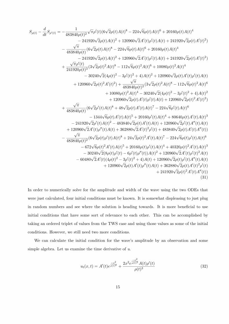
In order to numerically solve for the amplitude and width of the wave using the two ODEs that

were just calculated, four initial conditions must be known. It is somewhat displeasing to just plug

in random numbers and see where the solution is heading towards. It is more beneficial to use

initial conditions that have some sort of relevance to each other. This can be accomplished by

taking an ordered triplet of values from the TWS case and using those values as some of the initial

conditions. However, we still need two more conditions.

We can calculate the initial condition for the wave’s amplitude by an observation and some

simple algebra. Let us examine the time derivative of u.

ut(x, t) = A′(t)e−x2

ρ(t)2 +2x2e

−x2

ρ(t)2 A(t)ρ′(t)

ρ(t)3(32)

15

Observe that

x =ρ(0)√

2(33)

is an inflection point of u(x,t) and

ut(x, 0) ≈ c (34)

(34) holds true since ut represents how fast the wave is moving with respect to time, which is the

same as the wave speed.

Using the data

t = 0 (35)

x =ρ(0)√

2(36)

A(0) = A (37)

ρ(0) = ρ (38)

ut(x, 0) = c (39)

where A, ρ, c are chosen values from the TWS trial earlier, we can calculate the relationship

between A′(0) and ρ′(0). Plugging these substitutions into (32) yields

A′(0) = c√e− A

ρρ′(0) (40)

where ρ(0) is some constant, say k, that is chosen carefully to yield reasonable results. With these

values, A(t) and ρ(t) can be numerically calculated.

By choosing

c = .25 (41)

k = .3557619989 (42)

we establish a relationship between the wave’s amplitude and width, shown in Figure 6.

16

1 2 3 4 5Time

2

4

6

8

10

Width

Amplitude

Figure 6: G Trial DWS Sine-Gordon: Amplitude and width as functions of time.

By plugging these numerical values into our trial function we obtain a wave changing over time,

represented by Figure 7.

17

-6 -4 -2 2 4 6x

-1

1

2

3

4

5

6u

-6 -4 -2 2 4 6x

-1

1

2

3

4

5

6u

-6 -4 -2 2 4 6x

-1

1

2

3

4

5

6u

-6 -4 -2 2 4 6x

-1

1

2

3

4

5

6u

-6 -4 -2 2 4 6x

-1

1

2

3

4

5

6u

Figure 7: G Trial DWS Sine-Gordon: Wave at times t=0,1,2,3,4 respectively (left to right, top to

bottom)

.

18

3.2 Odd Oriented Gaussian Wave Trial Function

There is a set of solutions that do not resemble the trial that was previously being used. This other

trial function can be thought of as a Gaussian wave oriented as an odd function, hence the title.

3.2.1 Traveling Wave Solution

With a slight modification, and the Lorentzian transformation, the new trial function that will be

used is

u(ξ) = −Aξe−ξ2

ρ2 (43)

Once again we have the Lagrangian

L =1

2(1− c2)(u′)2 +

u2

2!− u4

4!+

u6

6!− u8

8!(44)

Hence the action is

S =A2√πρ(1528823808

√2(1− c2) + 509607936

√2ρ2 − 7962624A2ρ4 + 16384

√6A4ρ6 − 81

√2A6ρ8)

8153726976

(45)

The two Euler Lagrange equations become

(46)∂S

∂A=

A2√πρ(−15925248Aρ4 + 65536√6A3ρ6 − 486

√2A5ρ8)

8153726976

+A√πρ(1528823808

√2(1− c2) + 509607936

√2ρ2 − 7962624A2ρ4 + 16384

√6A4ρ6 − 81

√2A6ρ8)

4076863488

∂S

∂ρ=

A2√πρ(1019215872√2ρ− 31850496A2ρ2 + 98304

√6A4ρ5 − 648

√2A6ρ7)

8153726976

+A2√π(1528823808

√2(1− c2) + 509607936

√2ρ2 − 7962624A2ρ4 + 16384

√6A4ρ6 − 81

√2A6ρ8)

8153726976(47)

Once again, letting the wave speed vary, we can solve for the amplitude and width, represented in

Figure 8.

19

0.0 0.2 0.4 0.6 0.8 1.00

2

4

6

8

10

Figure 8: OOG Trial TWS Sine-Gordon: Amplitude and width paired with speed.

3.2.2 Dynamic Solution

Similar to the Gaussian wave trial function earlier, we will account for varying parameters, i.e.

parameters as functions of time, for which we shall add on another parameter called the center

line position. This new parameter, denoted by ζ, will try to monitor the acceleration of the wave

during it’s movement.

The new trial function to be tested is:

u(x, t) = −A(t)xe−(x−ζ(t))2

ρ(t)2 (48)

The Lagrangian for the dynamically changing Sine-Gordon Wave is

L =−1

2u2t +

1

2u2x +

u2

2!− u4

4!+

u6

6!− u8

8!(49)

20

The following action can be calculated

S = −√π

285380444160ρ(t)(17836277760

√2A(t)ρ(t)A′(t)(8ζ(t)ρ(t)ζ ′(t) + 4ζ(t)2ρ′(t) + 3ρ(t)2ρ′(t))

+ 17836277760√2ρ(t)2A′(t)2(4ζ(t)2 + ρ(t)2)

− 4459069440√2A(t)2(4ζ(t)2(−4ζ ′(t)2 − 3ρ′(t)2 + 4ρ(t)2 + 4)− 48ζ(t)ρ(t)ζ ′(t)ρ′(t)

+ ρ(t)2(−12ζ ′(t)2 − 15ρ′(t)2 + 4ρ(t)2 + 12))

+27√2A(t)8ρ(t)2(114688ζ(t)6ρ(t)2+53760ζ(t)4ρ(t)4+6720ζ(t)2ρ(t)6+65536ζ(t)8+105ρ(t)8)

− 114688√6A(t)6ρ(t)2(720ζ(t)4ρ(t)2 + 180ζ(t)2ρ(t)4 + 576ζ(t)6 + 5ρ(t)6)

+ 92897280A(t)4(48ζ(t)2ρ(t)4 + 64ζ(t)4ρ(t)2 + 3ρ(t)6))

(50)

21

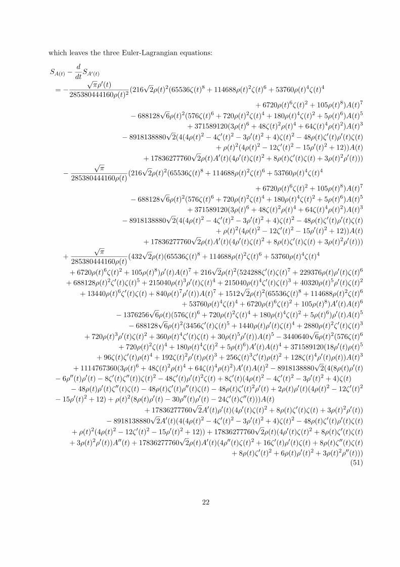
which leaves the three Euler-Lagrangian equations:

SA(t) −d

dtSA′(t)

= −√πρ′(t)

285380444160ρ(t)2(216

√2ρ(t)2(65536ζ(t)8 + 114688ρ(t)2ζ(t)6 + 53760ρ(t)4ζ(t)4

+ 6720ρ(t)6ζ(t)2 + 105ρ(t)8)A(t)7

− 688128√6ρ(t)2(576ζ(t)6 + 720ρ(t)2ζ(t)4 + 180ρ(t)4ζ(t)2 + 5ρ(t)6)A(t)5

+ 371589120(3ρ(t)6 + 48ζ(t)2ρ(t)4 + 64ζ(t)4ρ(t)2)A(t)3

− 8918138880√2(4(4ρ(t)2 − 4ζ ′(t)2 − 3ρ′(t)2 + 4)ζ(t)2 − 48ρ(t)ζ ′(t)ρ′(t)ζ(t)

+ ρ(t)2(4ρ(t)2 − 12ζ ′(t)2 − 15ρ′(t)2 + 12))A(t)

+ 17836277760√2ρ(t)A′(t)(4ρ′(t)ζ(t)2 + 8ρ(t)ζ ′(t)ζ(t) + 3ρ(t)2ρ′(t)))

−√π

285380444160ρ(t)(216

√2ρ(t)2(65536ζ(t)8 + 114688ρ(t)2ζ(t)6 + 53760ρ(t)4ζ(t)4

+ 6720ρ(t)6ζ(t)2 + 105ρ(t)8)A(t)7

− 688128√6ρ(t)2(576ζ(t)6 + 720ρ(t)2ζ(t)4 + 180ρ(t)4ζ(t)2 + 5ρ(t)6)A(t)5

+ 371589120(3ρ(t)6 + 48ζ(t)2ρ(t)4 + 64ζ(t)4ρ(t)2)A(t)3

− 8918138880√2(4(4ρ(t)2 − 4ζ ′(t)2 − 3ρ′(t)2 + 4)ζ(t)2 − 48ρ(t)ζ ′(t)ρ′(t)ζ(t)

+ ρ(t)2(4ρ(t)2 − 12ζ ′(t)2 − 15ρ′(t)2 + 12))A(t)

+ 17836277760√2ρ(t)A′(t)(4ρ′(t)ζ(t)2 + 8ρ(t)ζ ′(t)ζ(t) + 3ρ(t)2ρ′(t)))

+

√π

285380444160ρ(t)(432

√2ρ(t)(65536ζ(t)8 + 114688ρ(t)2ζ(t)6 + 53760ρ(t)4ζ(t)4

+ 6720ρ(t)6ζ(t)2 + 105ρ(t)8)ρ′(t)A(t)7 + 216√2ρ(t)2(524288ζ ′(t)ζ(t)7 + 229376ρ(t)ρ′(t)ζ(t)6

+ 688128ρ(t)2ζ ′(t)ζ(t)5 + 215040ρ(t)3ρ′(t)ζ(t)4 + 215040ρ(t)4ζ ′(t)ζ(t)3 + 40320ρ(t)5ρ′(t)ζ(t)2

+ 13440ρ(t)6ζ ′(t)ζ(t) + 840ρ(t)7ρ′(t))A(t)7 + 1512√2ρ(t)2(65536ζ(t)8 + 114688ρ(t)2ζ(t)6

+ 53760ρ(t)4ζ(t)4 + 6720ρ(t)6ζ(t)2 + 105ρ(t)8)A′(t)A(t)6

− 1376256√6ρ(t)(576ζ(t)6 + 720ρ(t)2ζ(t)4 + 180ρ(t)4ζ(t)2 + 5ρ(t)6)ρ′(t)A(t)5

− 688128√6ρ(t)2(3456ζ ′(t)ζ(t)5 + 1440ρ(t)ρ′(t)ζ(t)4 + 2880ρ(t)2ζ ′(t)ζ(t)3

+ 720ρ(t)3ρ′(t)ζ(t)2 + 360ρ(t)4ζ ′(t)ζ(t) + 30ρ(t)5ρ′(t))A(t)5 − 3440640√6ρ(t)2(576ζ(t)6

+ 720ρ(t)2ζ(t)4 + 180ρ(t)4ζ(t)2 + 5ρ(t)6)A′(t)A(t)4 + 371589120(18ρ′(t)ρ(t)5

+ 96ζ(t)ζ ′(t)ρ(t)4 + 192ζ(t)2ρ′(t)ρ(t)3 + 256ζ(t)3ζ ′(t)ρ(t)2 + 128ζ(t)4ρ′(t)ρ(t))A(t)3

+ 1114767360(3ρ(t)6 + 48ζ(t)2ρ(t)4 + 64ζ(t)4ρ(t)2)A′(t)A(t)2 − 8918138880√2(4(8ρ(t)ρ′(t)

− 6ρ′′(t)ρ′(t)− 8ζ ′(t)ζ ′′(t))ζ(t)2 − 48ζ ′(t)ρ′(t)2ζ(t) + 8ζ ′(t)(4ρ(t)2 − 4ζ ′(t)2 − 3ρ′(t)2 + 4)ζ(t)

− 48ρ(t)ρ′(t)ζ ′′(t)ζ(t)− 48ρ(t)ζ ′(t)ρ′′(t)ζ(t)− 48ρ(t)ζ ′(t)2ρ′(t) + 2ρ(t)ρ′(t)(4ρ(t)2 − 12ζ ′(t)2

− 15ρ′(t)2 + 12) + ρ(t)2(8ρ(t)ρ′(t)− 30ρ′′(t)ρ′(t)− 24ζ ′(t)ζ ′′(t)))A(t)

+ 17836277760√2A′(t)ρ′(t)(4ρ′(t)ζ(t)2 + 8ρ(t)ζ ′(t)ζ(t) + 3ρ(t)2ρ′(t))

− 8918138880√2A′(t)(4(4ρ(t)2 − 4ζ ′(t)2 − 3ρ′(t)2 + 4)ζ(t)2 − 48ρ(t)ζ ′(t)ρ′(t)ζ(t)

+ ρ(t)2(4ρ(t)2 − 12ζ ′(t)2 − 15ρ′(t)2 + 12)) + 17836277760√2ρ(t)(4ρ′(t)ζ(t)2 + 8ρ(t)ζ ′(t)ζ(t)

+ 3ρ(t)2ρ′(t))A′′(t) + 17836277760√2ρ(t)A′(t)(4ρ′′(t)ζ(t)2 + 16ζ ′(t)ρ′(t)ζ(t) + 8ρ(t)ζ ′′(t)ζ(t)

+ 8ρ(t)ζ ′(t)2 + 6ρ(t)ρ′(t)2 + 3ρ(t)2ρ′′(t)))

(51)

22

Sρ(t) −d

dtSρ′(t) = Refer to Appendix 1 for Mathematica Code (52)

Sζ(t) −d

dtSζ′(t)

= −√πρ′(t)

285380444160ρ(t)2(27

√2ρ(t)2(524288ζ(t)7 + 688128ρ(t)2ζ(t)5 + 215040ρ(t)4ζ(t)3

+ 13440ρ(t)6ζ(t))A(t)8 − 114688√6ρ(t)2(3456ζ(t)5 + 2880ρ(t)2ζ(t)3 + 360ρ(t)4ζ(t))A(t)6

+ 92897280(96ζ(t)ρ(t)4 + 256ζ(t)3ρ(t)2)A(t)4

− 4459069440√2(8ζ(t)(4ρ(t)2 − 4ζ ′(t)2 − 3ρ′(t)2 + 4)− 48ρ(t)ζ ′(t)ρ′(t))A(t)2

+ 17836277760√2ρ(t)A′(t)(8ρ(t)ζ ′(t) + 8ζ(t)ρ′(t))A(t) + 142690222080

√2ζ(t)ρ(t)2A′(t)2)

−√π

285380444160ρ(t)(27

√2ρ(t)2(524288ζ(t)7 + 688128ρ(t)2ζ(t)5 + 215040ρ(t)4ζ(t)3

+ 13440ρ(t)6ζ(t))A(t)8 − 114688√6ρ(t)2(3456ζ(t)5 + 2880ρ(t)2ζ(t)3 + 360ρ(t)4ζ(t))A(t)6

+ 92897280(96ζ(t)ρ(t)4 + 256ζ(t)3ρ(t)2)A(t)4

− 4459069440√2(8ζ(t)(4ρ(t)2 − 4ζ ′(t)2 − 3ρ′(t)2 + 4)− 48ρ(t)ζ ′(t)ρ′(t))A(t)2

+ 17836277760√2ρ(t)A′(t)(8ρ(t)ζ ′(t) + 8ζ(t)ρ′(t))A(t) + 142690222080

√2ζ(t)ρ(t)2A′(t)2)

+

√π

285380444160ρ(t)(54

√2ρ(t)(524288ζ(t)7 + 688128ρ(t)2ζ(t)5 + 215040ρ(t)4ζ(t)3

+ 13440ρ(t)6ζ(t))ρ′(t)A(t)8

+ 27√2ρ(t)2(3670016ζ ′(t)ζ(t)6 + 1376256ρ(t)ρ′(t)ζ(t)5 + 3440640ρ(t)2ζ ′(t)ζ(t)4

+ 860160ρ(t)3ρ′(t)ζ(t)3 + 645120ρ(t)4ζ ′(t)ζ(t)2 + 80640ρ(t)5ρ′(t)ζ(t) + 13440ρ(t)6ζ ′(t))A(t)8

+ 216√2ρ(t)2(524288ζ(t)7 + 688128ρ(t)2ζ(t)5 + 215040ρ(t)4ζ(t)3 + 13440ρ(t)6ζ(t))A′(t)A(t)7

− 229376√6ρ(t)(3456ζ(t)5 + 2880ρ(t)2ζ(t)3 + 360ρ(t)4ζ(t))ρ′(t)A(t)6

− 114688√6ρ(t)2(17280ζ ′(t)ζ(t)4+5760ρ(t)ρ′(t)ζ(t)3+8640ρ(t)2ζ ′(t)ζ(t)2+1440ρ(t)3ρ′(t)ζ(t)

+ 360ρ(t)4ζ ′(t))A(t)6 − 688128√6ρ(t)2(3456ζ(t)5 + 2880ρ(t)2ζ(t)3 + 360ρ(t)4ζ(t))A′(t)A(t)5

+ 92897280(96ζ ′(t)ρ(t)4 + 384ζ(t)ρ′(t)ρ(t)3 + 768ζ(t)2ζ ′(t)ρ(t)2 + 512ζ(t)3ρ′(t)ρ(t))A(t)4

+ 371589120(96ζ(t)ρ(t)4 + 256ζ(t)3ρ(t)2)A′(t)A(t)3

− 4459069440√2(−48ζ ′(t)ρ′(t)2 − 48ρ(t)ζ ′′(t)ρ′(t) + 8ζ ′(t)(4ρ(t)2 − 4ζ ′(t)2 − 3ρ′(t)2 + 4)

− 48ρ(t)ζ ′(t)ρ′′(t) + 8ζ(t)(8ρ(t)ρ′(t)− 6ρ′′(t)ρ′(t)− 8ζ ′(t)ζ ′′(t)))A(t)2

+ 17836277760√2A′(t)ρ′(t)(8ρ(t)ζ ′(t) + 8ζ(t)ρ′(t))A(t)

− 8918138880√2A′(t)(8ζ(t)(4ρ(t)2 − 4ζ ′(t)2 − 3ρ′(t)2 + 4)− 48ρ(t)ζ ′(t)ρ′(t))A(t)

+ 17836277760√2ρ(t)(8ρ(t)ζ ′(t) + 8ζ(t)ρ′(t))A′′(t)A(t)

+ 17836277760√2ρ(t)A′(t)(16ζ ′(t)ρ′(t) + 8ρ(t)ζ ′′(t) + 8ζ(t)ρ′′(t))A(t)

+ 142690222080√2ρ(t)2A′(t)2ζ ′(t) + 285380444160

√2ζ(t)ρ(t)A′(t)2ρ′(t)

+ 17836277760√2ρ(t)A′(t)2(8ρ(t)ζ ′(t) + 8ζ(t)ρ′(t)) + 285380444160

√2ζ(t)ρ(t)2A′(t)A′′(t))

(53)

In order to solve this system of ODEs, there needs to be initial conditions, which can be obtained

by examining the Traveling Wave Solution, similar to the Gaussian Wave Trial case. We need to

23

choose a trio of values for the amplitude and width relative to speed to use as the initial conditions.

However, this only satisifies three out of the six initial conditions necessary. The third condition

that is met is the ζ ′(0) term which can be considered as the initial speed of the wave, in other

words

ζ ′(0) ≈ ut(x, 0) ≈ c (54)

Just like in the Gaussian trial case, we will allow ρ′(0) to be a pivot variable and choose values for

it that produce reasonable results. For the ζ(0) case, we need to be careful about what value to

start it at. It may not be obvious, but choosing ζ(0) = 0 is dangerous because undefined quantities

appear during the solving process, so we need to choose another value. It’s value must be something

relatable to the other conditions in some way, so we will choose a value to allow for simplicity in

some sort of calculation. Suppose

ζ(0) =ρ(0)√

2(55)

because this value is a critical point, which is easier to work with.

We will, once again, look at the time derivative of u

ut(x, t) = −A′(t)xe− (x−ζ(t))2

ρ(t)2 − xA(t)e− (x−ζ(t))2

ρ(t)2 (2(x− ζ(t))ζ ′(t)

ρ(t)2+

2(x− ζ(t))2ρ′(t)

ρ(t)3) (56)

to solve for A′(t). Using the data

t = 0 (57)

x = −ζ(0) (58)

ut(x, 0) = c (59)

A(0) = A (60)

ρ(0) = ρ (61)

ζ(0) =ρ(0)√

2(62)

ζ ′(0) = c (63)

24

we can solve for A′(0) in terms of ρ′(0). Plugging these substitutions into (56) gives the result:

A′(0) =

√2

ρe2c− A

ρ(4ρ′(0)− 2

√2c) (64)

where, again, ρ′(0) is some constant k.

We will choose

c = .1 (65)

k = .2 (66)

By numerically solving the three Ordinary Differential Equations with the initial conditions above,

we are able to find numerical values for A(t), ρ(t), and ζ(t) shown in Figure 9.

0.02 0.04 0.06 0.08

2

4

6

8

10

Center Line

Position

Width

Amplitude

Figure 9: OOG Trial DWS Sine-Gordon: Amplitude, width, and center line position as functions

of time

Plugging these numerical values back into the trial function yields the slideshow of pictures

depicted by Figure 7.

25

-10 -5 5 10 15x

-10

-8

-6

-4

-2

2u

-10 -5 5 10 15x

-10

-8

-6

-4

-2

2u

-10 -5 5 10 15x

-10

-8

-6

-4

-2

2u

Figure 10: G Trial DWS Sine-Gordon: Wave at times t=0,0.04,0.08 respectively (left to right, top

to bottom).

.

4 Conclusions/Future Research

The goal of the project was to simulate solitons in the Sine-Gordon equation using this approxi-

mation technique by utilizing a trial function that would be tested as a viable solution. However,

it appears that these solutions do not last very long, especially the odd-oriented Gaussian wave.

The solutions appear to be short lived because the Sine-Gordon equation is used for nanoscopic

physical systems, which means even having solutions that last milliseconds are reasonable solutions.

It is important to note that there are no units involved due to the generality of the application.

26

By examining the odd-oriented Gaussian wave trial function results, we see that the ζ term has

negligible change. This means the wave does not accelerate or deccelerate enough to notice, so the

ζ parameter is not necessary in future calculations.

For the future, there are many things that can be worked on in this project. Negative amplitudes

could be accounted for to avoid loss of generality. More values of speed can be tested/examined in

both trials to see if there are any other solutions besides what is in the interval between 0 and 1.

There is also the possibility of testing ρ′(0) values, that can be extended to 8 decimals, to look for

other solutions. Besides changing parameter values, we could even choose completely different trial

functions to find other sets of solutions. There still needs to be a comparison to an exact solution

to see how accurate the results really are. Based on how the trial function was formulated, the

frame of reference is centered on the moving soliton itself, so it appears to be standing still. To

account for this, one possible solution would be to let the x variable be dependent on time as well,

which will allow the wave to travel while having a still frame reference. Besides dealing with a

single soliton, there is the possibility of having multiple solitons. Hopefully these ideas can be put

to the test in future research.

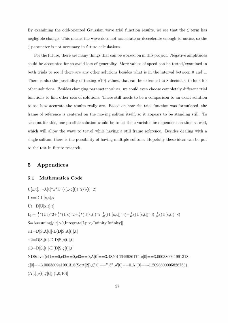
5 Appendices

5.1 Mathematica Code

U[x,t]:=-A[t]*x*Eˆ(-(x-ζ[t])ˆ2/ρ[t]ˆ2)

Ux=D[U[x,t],x]

Ut=D[U[x,t],t]

Lp=-12*(Ut)ˆ2+12*(Ux)ˆ2+1

2*(U[x,t])ˆ2-14!((U[x,t])ˆ4)+ 1

6!((U[x,t])ˆ6)- 18!((U[x,t])ˆ8)

S=Assuming[ρ[t]>0,Integrate[Lp,x,-Infinity,Infinity]]

el1=D[S,A[t]]-D[D[S,A[t]],t]

el2=D[S,[t]]-D[D[S,ρ[t]],t]

el3=D[S,[t]]-D[D[S,ζ[t]],t]

NDSolve[(el1==0,el2==0,el3==0,A[0]==3.485016648986174,ρ[0]==3.000380941991318,

ζ[0]==3.000380941991318(Sqrt[2]),ζ’[0]==”.5”,ρ’[0]==0,A’[0]==-1.2098800005826753),

(A[t],ρ[t],ζ[t]),(t,0,10)]

27

References

[1] D.J. Kaup, T.K. Vogel, Quantitative Measurement of Variational Approximations, Physics

Letters A PLA 362 (2007) 289-297

[2] J. David Logan Applied Mathematics. 2nd ed.

A Wiley-Interscience Publication. 1996.

[3] P.G. Drazin, R.S. Johnson Solitons: an introduction

Cambridge University Press. 1989.

[4] Daniel Zwillinger Handbook of Differential Equations 3rd ed.

Academic Press. 1998. p. 180

[5] http://mathworld.wolfram.com/Sine-GordonEquation.html

28