Ilian T. Iliev

CITA

with G. Mellema (Stockholm), U.-L. Pen, J.R. Bond (CITA), P. Shapiro and M. Alvarez (UT Austin)

Simulating Reionization at Large Scales: Progress and

Observability

The First Stars and Evolution of the Early Universe, Seattle, July 03-07, 2006

Talk outline: ➢What is required for simulations of global reionization

and making reliable observational predictions?➢Our simulations: method and basic results (Mellema,

Iliev, Shapiro, Alvarez, 2006, NewA, 11, 374; Iliev, Mellema, Pen, Merz,

Shapiro 2006, MNRAS, 369, 1625; Mellema, Iliev, Pen, Shapiro: astro-

ph/0603518) ➢Self-regulated reionization (Iliev, Mellema, Shapiro & Pen,

2006, in prep.)

➢kSZ from patchy reionization: first results (Iliev, Pen,

Bond, Mellema, & Shapiro, 2006 NewA Reviews and in prep.) ➢Redshifted 21-cm emission ( Mellema, Iliev, Pen, Shapiro:

astro-ph/0603518 and in prep.).

Requirements for Simulations of Global Reionization

➢Large computational boxes – due to strong bias of ionizing sources HII regions are large; need a degree scale on the sky and few MHz in bandwidth (redshifted 21-cm) for practical observational predictions.

➢Detailed knowledge of structures forming at high-z: ➢number and distribution of sources – down to dwarf galaxies

of ~108Msolar

➢density fluctuations (photon sinks) – either self-shielded (MH) or not.

➢Physical models for the ionizing sources (photon production, star-formation efficiencies, escape fractions)

➢Precise, high-resolution radiative transfer

• Very high resolution N-body simulations of structure formation using PMFAST code developed at CITA (Merz, Pen & Trac 2004)

• 100/h, 35/h and 3.5/h Mpc boxes, 16243

particles (4.3 billion), 32483 cells. Up to 1-2 million halos identified (with >100 particles/halo =2.5x109M

solar,

108 Msolar

and 105

M

solar )

High-z Structure Formation

z=10

The high-z halo mass function(Iliev, Mellema, Pen, Merz, Shapiro: astro-ph/0512187)

Up to ~2 million halos identified.

The simulated halo mass function at high z (z>10) is not matched well by either Sheth-Tormen (ST), or Press-Schechter analytical models.

However, below z~10 ST is a fairly good fit.

C2-Ray: Conservative, Causal Ray-tracing

of ionizing radiation

(Mellema,Iliev, Alvarez, Shapiro, NewA, 11, 374, 2006).

We have developed a new radiative transfer method: -explicitly photon-conserving.

-tested in detail, many tests had exact analytical solutions some of which we found for the first time.-correctly evolves I-fronts even at very low spatial and

time resolutions-non-equilibrium chemistry, energy equation

Fast and efficient, easily coupled to hydro and N-body dynamics, up to high resolutions

Applicable (and already applied) to both cosmological and non-cosmological problems.

Dynamical HII Region Evolution in Turbulent Molecular Clouds

(Mellema, Arthur, Henney, Iliev, Shapiro, ApJ, in press,

astro-ph/0512554)

Movie

How reliable are current radiative transfer codes? :

Cosmological radiative transfer code comparison project

(Iliev et al. 2006, astro-ph/0603199, MNRAS submitted)

➢ Verification of current codes➢ Testbed for future radiative transfer code

development➢ 11 codes➢ 8 tests, 5 pure RT and 3 with gas-dynamics➢ Paper I (pure radiative transfer, static density fields)

submitted. ➢ Results with gasdynamics still being collected and

studied, to be completed in the next few months.

Radiative transfer code comparison

project: Sample Results

Sample results: Classic HII region expansion, Stromgren sphere

Reionization Calculation(Iliev, Mellema, Pen, Merz, Shapiro: astro-ph/0512187; Mellema,

Iliev, Pen, Shapiro: astro-ph/0603518)

➢ We postprocess this volume (regridded to 2033, 4063 and 8123) with our radiative transfer code C2-Ray.

➢ 50-100 time-slices of density and corresponding halo lists (10-20 Myr between slices).

➢ Sources are all resolved halos. M/L=const, fixed (2000,250) photons/atom escaping (Iliev, Scannapieco & Shapiro 2005).

➢ Sub-grid gas clumping C(z) is also included, based on 3.5/h Mpc box PMFAST simulation.

➢ Small source suppression included: Jeans mass filtering.

Simulations

• Photon efficiency f = fSF x fesc x Nphoton

0.0978.210.8C(z)250f250C

τ esz

ovz(50%)clumpingfSim

0.1219.311.71250f250

0.13510.1512.6C(z)2000f2000C

0.14511.313.612000f2000

+ 8 more simulations with a smaller (50 Mpc) box, which allowes us to resolve ~108 M

solar halos; + 5 more with WMAP 3-year parameters

Self-Regulated Reionization Lower large-source

efficiencies, Jeans-mass filtering of small sources and time-increasing sub-grid gas clumping all extend reionization and delay overlap.

However:

Lower small-source efficiency does not extend reionization appreciably (but decreases τ ). Reionization is self-regulated.

Self-Regulated Reionization II

Jeans-mass filtering of small sources suppresses the total emissivity by order of magnitude or more.

However:

The epoch overlap is determined by the level of sub-grid clumping and the large, unsuppressed sources.

Reionization: WMAP1 vs. WMAP3(Alvarez et al. 2006,ApJL,644,101; Iliev et al., in prep.)

In WMAP3 cosmology reionization is delayed by 1.3-1.4 in 1+z, just enough to compensate for the new value of τ . Originally shown analytically, now confirmed by simulations.

Mean Ionized Fractions vs. Density: Inside-Out Reionization II

xm=mean mass-

weighted ion. fractionin a density bin

The highly overdense regions get ionized earliest, the lower the density, the later on average a region gets ionized.

Reionization history of sub-regionsgreen = total mean

red = mean-density

subregions

blue = all sub-regions

For small regions there is

huge scatter and overlap

epoch cannot be determined

well. Only sufficiently large

regions (>20 Mpc) describe

the mean evolution well

(though still larger volumes

needed for e.g. HII regions

size distribution).

Large-Scale Topology of Reionization: Animations

100/h Mpc box, 406^3 radiative transfer simulationEvolution: z=21 to 12.–HII regions of individual sources and groups start overlapping.–The topology of the ionized / neutral regions is complex.–At z=11 nearly the whole box is ionized (52,000 sources).

Large-Scale Topology of Reionization: Animations

35/h Mpc box, 406^3 radiative transfer simulationEvolution: z=30 to 10.

>108 solar mass halos resolved (i.e. all atomically-cooling halos)

Jeans mass filtering included

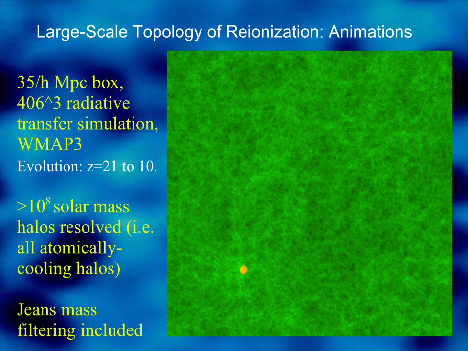
Large-Scale Topology of Reionization: Animations

35/h Mpc box, 406^3 radiative transfer simulation, WMAP3Evolution: z=21 to 10.

>108 solar mass halos resolved (i.e. all atomically-cooling halos)

Jeans mass filtering included

Evolution Slicesf250

Evolution Slices: WMAP3f250

Density Power Spectra of H I and H II regions

solid = density

dashed = HII density

dotted = HI density

Size distribution of the HII regionsTop: bubble numbersBottom: volume filling factors

Note the characteristic double-peaked distributions:1st peak: local source clust.2nd peak: percolation of the bubbles

kSZ from patchy reionization(Iliev, Pen, Mellema, Bond, & Shapiro, NewA Rev. 2006, in

press and in prep.)• Temperature variations given by LOS integral:

• Method: – find all integrals along LOS for available outputs

– every light-crossing time interpolate between closest two outputs

– to avoid periodicity artefacts change directions (x-y-z) and do random translations (using box periodicity) and/or 90 degree rotations

Sample kSZ map from patchy reionization

➢Sample kSZ map (run f250C).

➢ range of pixel values is ∆T/T=-10-5 to 10-5 , i.e. ∆T max/min are in the tens of µK at ~ arcmin scales.

~1 deg

~1deg

(images produced using Ifrit package of N. Gnedin)

kSZ sky maps: early vs. extended reionization

f250 f2000

f250C f2000C

kSZ sky maps: extended vs. instant reionization

f250 instant reionization, same τ

kSZ sky maps: extended vs. uniform reionization

f250 uniform reionization, same xm (and τ )

kSZ sky power spectra➢ Power spectra peak at l~3000-5000,

with a peak value of a few µK

➢ Early and late reionization scenarios

(f2000, f2000C, f250 and f250C):

would be difficult to distinguish

(some differences for l>10,000,

especially for very extended

reionization, f250C)

➢ Instant reionization (at z~13, same τ

as f250) has ~ order of magnitude

less power for l~2000-8000, but

same large-l behaviour.

➢ Uniform reionization (same xm as

f250) has much less power for all l's.

20 Mpc

kSZ non-Gaussianity?• Maps are fairly Gaussian, but

presence of more clumping

introduces significant non-

Gaussianity at wings

solid: simulations

dotted: Gaussian with the same

mean and rms

kSZ sky power spectra➢ Power spectra peak at l~3000-5000,

with a peak value of a few µK

➢ Early and late reionization scenarios

(f2000, f2000C, f250 and f250C):

would be difficult to distinguish

(some differences for l>10,000,

especially for very extended

reionization, f250C)

➢ Instant reionization (at z~13, same τ

as f250) has ~ order of magnitude

less power for l~2000-8000, but

same large-l behaviour.

➢ Uniform reionization (same xm as

f250) has much less power for all l's.

20 Mpc

kSZ sky power spectra: comparison with analytical results

(from Gruzinov and Hu 1998, McQuinn et al. 2005)

extended

rapid

uniform

GH

kSZ sky power spectra: comparison with

analytical results II

Santos et al. (solid, left) also find a similar maximum signal, though power spectra drop much more slowly at high-l. Difference is probably due to the ionizing source clustering in simulations.

21-cm: What Will We Observe?(Mellema, Iliev, Pen, Shapiro: astro-ph/0603518)

• Frequency Redshift Time.

• Observations of fields ∆θ∆θ over ∆ν: image cube.

• Signal too weak?• Statistical measurements:

– Global signal.

– Power spectra (visibilities).

– Non-Gaussian featuresz

ν

θ

time θ

Ob

serv

er

Constructing the 21cm Signal

We assume that the neutral IGM has TS >>TCMB :

– heated by X-rays

– Ts easily coupled to Tk by Ly-α (Ciardi & Madau 2004).

In this case,

δ T(z) ≈ 27 xHI (1 + δ )[(1+z)/10]1/2 mK

depends on overdensity (δ ) and neutral fraction (xHI).

Image Cube: Evolution Slice

z

ν

time θ

θ

Line spectra: effect of redshift distortions

With redshift distortions With redshift distortions –

no redshift distortions

f250

LOS spectra: smoothed vs. high-resolution

Full resolution Beam & Bandwidth smoothed: 3’, 0.2 MHz

f250

Image Cube: Image Slice

z

time

Beam and UV coverage

Comp. Gaussian

Gaussian

Tophat

UV Coverage of LOFAR Virtual Core

Compensated Gaussian mimics UV coverage of compact interferometer

Different Beam shapes

Gaussian

Beam

Compensated

Gaussian

Beam

f2000

Global Step

• Average signal over all lines of sight:

global step (Shaver et al. 1999). Sharp

change with frequency.

• Simulations show gradual transition,

instead:~20 mK over ~20 MHz.

WMAP1

WMAP3

WMAP1:left to right: f250C, f250, f2000C,f2000)

WMAP3: left to right: f250C, f250_250S,

f2000C_250S, f2000_250S)

RMS Fluctuations

➢ All fluctuations peak at ~50% ionization.

➢ Max amplitude decreases/increases

depending on how well the beam and

bandwidth match the typical patch sizes.

➢ C(z) results in broader peak

➢ Interferometer measures diff. temperatures.

➢ Expressed as one number: rms fluctuations.

➢ Small boxes underestimate the fluctuations!

WMAP1

WMAP3

Angular (2D) Power spectra

• Decompose maps in spherical harmonics Ylm.

• Power spectrum of multipole moments l: l(l+1)Cl/2π.

• Peak shifts from high to low l during reionization.

Strongest signal: peaks at l=5000 (4’).

f250

Beyond Gaussian statistics

• What is the brightest point in our volume at a given redshift?

⟨δT⟩ ⟨δT⟩/⟨xHI⟩

δTmax (full resolution)

δTmax (1’, 0.1 MHz)

δTmax (3’, 0.2 MHz)

δTmax (6’, 0.4 MHz)

Probability Distribution Functions

Distribution of δT is highly non-Gaussian, especially at late times.

Gaussian (20/h Mpc) Gaussian (10/h Mpc)

Gaussian (5/h Mpc)

PDF (20 Mpc/h) PDF (10 Mpc/h) PDF (5 Mpc/h)

f250

GP Optical Depth

solid=mediandotted=meandashed=rms

Conclusions➢ Now we can do sufficiently large (100/h Mpc size) radiative transfer

simulations of reionization to reliably derive the global reionization history, HII

region size distributions, redshifted 21-cm signal, patchy kSZ effect, etc.

➢ Reionization proceeds inside-out and is strongly self-regulated.

➢ Small-volume simulations can give very incorrect results for global process.

➢ The kSZ power spectra peak strongly to l(l+1)cl/2π > 10 (µK)2 at l~3-9000.

High sub-grid gas clumping introduces non-Gaussian features in the maps.

➢ The patchy kSZ signal is much stronger than the instant or uniform one.

➢ Realistic extended reionization scenarios difficult to distinguish from each

other based solely on kSZ, need to combine with other observables.

➢ Global 21-cm step is gradual, difficult to observe. Fluctuations should be

observable and peak at ~50% ionization. Redshift spectral distortions are

important. Late-time PDFs are strongly non-Gaussian.

➢ Lowering source efficiency and increasing gas clumping both extend

reionization and delay overlap, but have little impact on 21-cm observables.

➢ Small-box simulations significantly underpredict 21-cm and kSZ signals.