Simulating effects of land use changes on carbon … · Simulating effects of land use changes on...
21
Tellus (2008), 60B, 583–603 C 2008 The Authors Journal compilation C 2008 Blackwell Munksgaard Printed in Singapore. All rights reserved TELLUS Simulating effects of land use changes on carbon fluxes: past contributions to atmospheric CO 2 increases and future commitments due to losses of terrestrial sink capacity By K. M. STRASSMANN 1∗ , F. JOOS 1 andG. FISCHER 2 , 1 Climate and Environmental Physics, Physics Institute, University of Bern, Bern, Switzerland; 2 International Institute for Applied Systems Analysis, A-2361 Laxenburg, Austria (Manuscript received 31 June 2007; in final form 20 December 2007) ABSTRACT The impact of land use on the global carbon cycle and climate is assessed. The Bern carbon cycle-climate model was used with land use maps from HYDE3.0 for 1700 to 2000 A.D. and from post-SRES scenarios for this century. Cropland and pasture expansion each cause about half of the simulated net carbon emissions of 188 Gt C over the industrial period and 1.1 Gt C yr −1 in the 1990s, implying a residual terrestrial sink of 113 Gt C and of 1.8 Gt C yr −1 , respectively. Direct CO 2 emissions due to land conversion as simulated in book-keeping models dominate carbon fluxes due to land use in the past. They are, however, mitigated by 25% through the feedback of increased atmospheric CO 2 stimulating uptake. CO 2 stimulated sinks are largely lost when natural lands are converted. Past land use change has eliminated potential future carbon sinks equivalent to emissions of 80–150 GtC over this century. They represent a commitment of past land use change, which accounts for 70% of the future land use flux in the scenarios considered. Pre-industrial land use emissions are estimated to 45 Gt C at most, implying a maximum change in Holocene atmospheric CO 2 of 3 ppm. This is not compatible with the hypothesis that early anthropogenic CO 2 emissions prevented a new glacial period. 1. Introduction Past and current land use and land use changes (LULUC) con- tribute to the ongoing anthropogenic climate change (Forster et al., 2007). LULUC activities continue to cause large emis- sions of carbon dioxide (Houghton et al., 1983; McGuire et al., 2001; Achard et al., 2002; DeFries et al., 2002; Houghton, 2003) and other greenhouse gases (Strengers et al., 2004) to the at- mosphere and alter surface properties such as albedo and wa- ter vapour exchange (Feddema et al., 2005; Sitch et al., 2005). Presently, about 40% of the world’s vegetated land surface (ex- cluding deserts, barren and ice-covered land) is used as cropland or pasture (Klein Goldewijk, 2001). While land use change has many socio-economic and climatic consequences, here, we are interested in the impact of LULUC on the global carbon cycle and atmospheric CO 2 and CO 2 related climatic changes over the industrial period and the future. ∗ Corresponding author. e-mail: [email protected] DOI: 10.1111/j.1600-0889.2008.00340.x Uncertainties in the quantitative understanding of the impact of LULUC on the global carbon cycle lead to uncertainties in projections of atmospheric CO 2 and climate, and consequently, affect the formulation of emission mitigation strategies. Carbon fluxes due to LULUC constitute the least well quantified flux in the global carbon budget (Pacala et al., 2001; Prentice et al., 2001; Goodale et al., 2002; Houghton et al., 2004; Denman et al., 2007). Carbon emissions from LULUC have traditionally been esti- mated by a book-keeping method (Houghton et al., 1983) that takes into account temporal delays between carbon emissions and uptake after deforestation or abandonment of used land. This approach neglects any feedback between atmospheric CO 2 , cli- mate and carbon emissions from LULUC (Leemans et al., 2002). Changes in management practices such as fire suppression, thin- ning or grazing (Hurtt et al., 2002; Nabuurs et al., 2003; Field and Raupach, 2004; Vesala et al., 2005) are often neglected, too. Carbon fluxes due to LULUC estimated with book-keeping methods have been used in coupled carbon cycle-climate mod- els (Prentice et al., 2001; Meehl et al., 2007). LULUC fluxes were exogenously prescribed in analogy to fossil emissions. It has been postulated that land carbon storage is overestimated in Tellus 60B (2008), 4 583 PUBLISHED BY THE INTERNATIONAL METEOROLOGICAL INSTITUTE IN STOCKHOLM SERIES B CHEMICAL AND PHYSICAL METEOROLOGY
Transcript of Simulating effects of land use changes on carbon … · Simulating effects of land use changes on...
Tellus (2008), 60B, 583–603 C© 2008 The AuthorsJournal compilation C© 2008 Blackwell Munksgaard
Printed in Singapore. All rights reservedT E L L U S
Simulating effects of land use changes on carbon fluxes:past contributions to atmospheric CO2 increases
and future commitments due to losses of terrestrialsink capacity
By K. M. STRASSMANN 1∗, F. JOOS 1 and G. FISCHER 2, 1Climate and Environmental Physics,Physics Institute, University of Bern, Bern, Switzerland; 2International Institute for Applied Systems Analysis, A-2361
Laxenburg, Austria
(Manuscript received 31 June 2007; in final form 20 December 2007)
ABSTRACTThe impact of land use on the global carbon cycle and climate is assessed. The Bern carbon cycle-climate model wasused with land use maps from HYDE3.0 for 1700 to 2000 A.D. and from post-SRES scenarios for this century. Croplandand pasture expansion each cause about half of the simulated net carbon emissions of 188 Gt C over the industrial periodand 1.1 Gt C yr−1 in the 1990s, implying a residual terrestrial sink of 113 Gt C and of 1.8 Gt C yr−1, respectively. DirectCO2 emissions due to land conversion as simulated in book-keeping models dominate carbon fluxes due to land use inthe past. They are, however, mitigated by 25% through the feedback of increased atmospheric CO2 stimulating uptake.CO2 stimulated sinks are largely lost when natural lands are converted. Past land use change has eliminated potentialfuture carbon sinks equivalent to emissions of 80–150 Gt C over this century. They represent a commitment of pastland use change, which accounts for 70% of the future land use flux in the scenarios considered. Pre-industrial land useemissions are estimated to 45 Gt C at most, implying a maximum change in Holocene atmospheric CO2 of 3 ppm. Thisis not compatible with the hypothesis that early anthropogenic CO2 emissions prevented a new glacial period.
1. Introduction
Past and current land use and land use changes (LULUC) con-tribute to the ongoing anthropogenic climate change (Forsteret al., 2007). LULUC activities continue to cause large emis-sions of carbon dioxide (Houghton et al., 1983; McGuire et al.,2001; Achard et al., 2002; DeFries et al., 2002; Houghton, 2003)and other greenhouse gases (Strengers et al., 2004) to the at-mosphere and alter surface properties such as albedo and wa-ter vapour exchange (Feddema et al., 2005; Sitch et al., 2005).Presently, about 40% of the world’s vegetated land surface (ex-cluding deserts, barren and ice-covered land) is used as croplandor pasture (Klein Goldewijk, 2001). While land use change hasmany socio-economic and climatic consequences, here, we areinterested in the impact of LULUC on the global carbon cycleand atmospheric CO2 and CO2 related climatic changes over theindustrial period and the future.
∗Corresponding author.e-mail: [email protected]: 10.1111/j.1600-0889.2008.00340.x
Uncertainties in the quantitative understanding of the impactof LULUC on the global carbon cycle lead to uncertainties inprojections of atmospheric CO2 and climate, and consequently,affect the formulation of emission mitigation strategies. Carbonfluxes due to LULUC constitute the least well quantified fluxin the global carbon budget (Pacala et al., 2001; Prentice et al.,2001; Goodale et al., 2002; Houghton et al., 2004; Denman et al.,2007).
Carbon emissions from LULUC have traditionally been esti-mated by a book-keeping method (Houghton et al., 1983) thattakes into account temporal delays between carbon emissionsand uptake after deforestation or abandonment of used land. Thisapproach neglects any feedback between atmospheric CO2, cli-mate and carbon emissions from LULUC (Leemans et al., 2002).Changes in management practices such as fire suppression, thin-ning or grazing (Hurtt et al., 2002; Nabuurs et al., 2003; Fieldand Raupach, 2004; Vesala et al., 2005) are often neglected, too.
Carbon fluxes due to LULUC estimated with book-keepingmethods have been used in coupled carbon cycle-climate mod-els (Prentice et al., 2001; Meehl et al., 2007). LULUC fluxeswere exogenously prescribed in analogy to fossil emissions. Ithas been postulated that land carbon storage is overestimated in
Tellus 60B (2008), 4 583
P U B L I S H E D B Y T H E I N T E R N A T I O N A L M E T E O R O L O G I C A L I N S T I T U T E I N S T O C K H O L M
SERIES BCHEMICALAND PHYSICAL METEOROLOGY
584 K. M. STRASSMANN ET AL.
such simulations, since no correction is made for the increas-ing area under cultivation, where carbon turnover is faster andsink capacity reduced compared to area covered by forests (Gitzand Ciais, 2004). This limitation can be overcome by endoge-nous modelling of LULUC processes based on spatially explicitland use maps. Previous global studies taking this approach usedterrestrial models either forced by prescribed climate fields andatmospheric CO2 (McGuire et al., 2001) or run as a module incoupled carbon cycle-climate model (e.g., Leemans et al., 2002;Sitch et al., 2005; Brovkin et al., 2006). Except Leemans et al.(2002), these studies considered changes in cropland and ne-glected the impact of changes in pasture area.
These studies highlight the importance of accurate spatiallyexplicit fields that describe the spatio-temporal evolution of thearea under land use for assessing LULUC impacts. Such mapshave recently become available for cropland (Ramankutty andFoley, 1999) and for cropland, pasture and built-up area (KleinGoldewijk, 2001, 2005; Klein Goldewijk and van Drecht, 2006)for the industrial period. Land use maps are also part of the outputof some integrated assessment models used to develop mitigationand non-mitigation emission scenarios (Nakicenovic and Swart,2000; Strengers et al., 2004; Riahi et al., 2007) for the 21stcentury. In combination, these products provide the opportunityto study the evolution of land use, atmospheric CO2 and climateover the industrial period and this century in a consistent way(Strengers et al., 2004).
Recently, a new set of emission scenarios have become avail-able that incorporate the latest progress in scenario development(Riahi et al., 2007). In addition to these plausible scenarios, IPCCillustrates in its Fourth Assessment Report inertia in the climatesystem by analysing the commitment of past and 21st centuryemissions on future climate (Meehl et al., 2007). In these com-mitment scenarios either radiative forcing is kept at the valuereached in year 2000 (or year 2100), or emissions are instan-taneously reduced to zero in 2000 (or 2100). In none of theseanalyses, the inertia of LULUC processes has been addressed.
Here, we apply the Bern Carbon Cycle-Climate (BernCC)model (Joos et al., 2001; Gerber et al., 2003, 2004; Joos et al.,2004) that includes the Lund-Potsdam-Jena Dynamic GlobalVegetation Model (LPJ-DGVM) (Sitch et al., 2003) comple-
1700 1800 1900 2000 2100Time (yr)
0
5
10
15
20
25
30
CO
2 E
mis
sio
n (
Gt
C/y
r)
A2B1B2
1700 1800 1900 2000 2100Time (yr)
0
10
20
30
40
50
60
LU
are
a (M
io k
m2)
A2B1B2no pasture
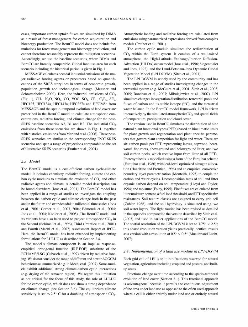
Fig. 1. Left-hand side: global land use areafor past 300 yrs and scenarios A2, B1 andB2. Right-hand side: CO2 emissions fromfossil fuel use and cement productionestimated for the industrial period (Marlandet al., 2006) and projected for this centuryfor the IIASA scenarios A2, B1 and B2.
mented with a new module describing LULUC processes to ad-dress a range of LULUC related research questions. The mostrecent maps from the History Database of the Global Environ-ment (Klein Goldewijk and van Drecht, 2006) and from the mostrecent post-SRES scenarios from the Institute of Applied Sys-tem Analyses (Riahi et al., 2007) are used to force the BernCCmodel. The BernCC model is cost-efficient, allowing us to per-form a complete set of sensitivity simulations used to disentanglequalitatively different processes contributing to the LULUC im-pact and to quantify their relative importance over time.
The goals of this study are: (i) to estimate carbon emissionsfrom LULUC over the industrial period and the past decades inthe BernCC model framework, thereby contributing to the ongo-ing assessment of the magnitudes und uncertainties of LULUCinduced carbon fluxes; (ii) to make an appraisal of the potentialimpact of pre-industrial LULUC on atmospheric CO2 and cli-mate; (iii) to project atmospheric CO2 and climate in three newscenarios for 21st century land use and emissions of CO2 andother anthropogenic forcing agents; (iv) to quantify the differ-ent environmental feedbacks and interactions of LULUC withpast and future atmospheric CO2 employing a range of factorialmodel experiments and (v) to assess the impact of past LULUCon future atmosphere-land carbon fluxes, atmospheric CO2, andclimate. We invoke the concept of a land use commitment tocharacterize this impact.
2. Methods
Sections 2.1 and 2.2 describe the boundary conditions used todrive the simulations (Fig. 1). These include estimates of pastLULUC and scenarios of LULUC and industrial emissions forthis century. The data provided by other research groups wereprocessed for use within BernCC as detailed below. Sections2.3–2.5 explain key model features and simulation procedures.Section 2.6 describes an analytical framework for decomposingthe impact of LULUC into qualitatively different processes.
2.1. Land use data
The HYDE database (version 3.0) from Klein Goldewijk and vanDrecht (2006) describes the geographically explicit evolution of
Tellus 60B (2008), 4
EFFECT OF LAND USE ON CARBON FLUXES 585
croplands, of pastures and of urban (built-up) areas for the pe-riod from 1700 to 2000. The urban land class was not included inthe previous HYDE2.0 database (Klein Goldewijk, 2001). TheHYDE data have a resolution of 5 arcmin in space and of 10 yr intime. For the future, the Land Use Change (LUC) group at IIASAhas developed maps of cropland and built-up area for a range of(updated, post-SRES) emissions scenarios based on the SRESstorylines (Tubiello and Fischer, 2006). The land use distribu-tion for year 2000 is derived from remote sensing satellite prod-ucts from the National Oceanic and Atmospheric AdministrationAdvanced Very High Resolution Radiometer (NOAA-AVHRR)and from the Global Land Cover Project (GLC2000) (Tubielloand Fischer, 2006). A map is supplied for each decade until2100 based on global food demand and supply simulations withIIASA’s linked agroecological zones (AEZ) model and worldfood system (BLS) model (Tubiello and Fischer, 2006). Data aregiven as cropland and built-up area fractions for each grid cellof 0.5◦ × 0.5◦. The evolution of pasture is not specified by theIIASA data.
The data are aggregated onto the BernCC model grid of 3.75◦
longitude by 2.5◦ latitude. The area fractions occupied by pasturep, cropland c and built-up area b (identified with the urban classin HYDE3.0) are specified for each cell. Only the net land usechanges on the grid cell level are modelled. Consequently, whennew land is claimed while used land is abandoned within thesame aggregated cell, the model ‘sees’ a net change smaller thanthe area experiencing land use change. In this way, about 15%of gross land use change is masked by the aggregation. The cor-responding bias to carbon fluxes should be smaller, since lossesfrom reclaimed land will be partly compensated by regrowth onabandoned land. The total land area in the coarse model gridis slightly smaller than that of the original map. Land use areawas conserved in the aggregation to prevent a bias on the rates ofland use change. Consequently, the percentage of the global landcover under land use is increased in the process (37% instead of33% in 2000 A.D.).
The land use data from HYDE3.0 and IIASA are combinedinto a land use evolution that exhibits a seamless transition be-tween the HYDE and IIASA data sets, as discontinuities wouldlead to spurious carbon fluxes. The land use distribution for year2000 is well established from satellite data and ground truth andis kept unchanged in the combined land use data set. The IIASAscenarios, consistent with the year 2000 data are also used with-out further modification. The HYDE data for the past, which aremore uncertain than the present land use map, are adjusted toblend in with the IIASA data at year 2000. Test simulations withthe original HYDE3.0 data yield very similar results with respectto global carbon fluxes and climate as the simulations with theadjusted data. The specific adjustment procedure is as follows.
The cropland fraction c is calculated as
c(t) = min
[1, cIIASA(2000) · cHYDE(t)
cHYDE(2000)
]∀ t < 2000. (1)
Thus, the spatial pattern is taken from the IIASA map at 2000, andthe history of each cell is scaled according to the HYDE data. Theminimum condition is necessary because in some cells, croplandhas a maximum in the past which may become greater thanunity when scaled with the IIASA map of 2000. In cells wherecropland exists in the IIASA map but not in the HYDE map,this approach is not applicable. Here, the latitudinally nearestcropland cell from HYDE was used for scaling.
A similar procedure was applied for cells with built-up areasin both data sets,
b(t) = min
[1 − c(t), bIIASA(2000) · bHYDE(t)
bHYDE(2000)
]
∀ t < 2000, (2)
where b is restricted to the area not already occupied by c. Built-up areas are sparse and the scaling procedure applied to croplandcould not be used for cells lacking built-up areas in HYDE.Instead, these cells were scaled using average HYDE built-updensities, calculated on a very coarse grid of 30 × 30 degrees tocapture the basic differences in the timing of development.
The evolution of pasture was taken directly from the HYDE3.0data, as the IIASA data do not contain information about pastures
p(t) = min[1 − c(t) − b(t), pHYDE(t) ] ∀ t ≤ 2000 , (3)
again with the condition that the combined area fractions c + b +p do not exceed unity. For times later than 2000, the same formulais used with pHYDE = pHYDE(2000). In other words, pasturesremain in continued use unless space is required for croplandor built-up area. We resort to this not very plausible assumptiondue to the lack of future scenarios of pasture development. Thisis clearly a limitation that should be addressed in future studies.The projected net change in the total area under land use (crop,pasture, built-up) is about 15% smaller than the net change incropland area. Often new cropland is assumed to be establishedon pasture land to meet the requirement that total land use areadoes not exceed the grid cell area.
Figure 1 shows the development of the global cropland andbuilt-up area and of pasture for the industrial period and for theIIASA scenarios A2, B1 and B2.
2.2. Emission and land cover scenarios
Emission scenarios for the SRES storylines A2, B1 and B2were developed at IIASA, running the MESSAGE model andthe DIMA model in a coupled mode (Rokityanskiy et al., 2006;Riahi et al., 2007). The DIMA and MESSAGE models simulateforestry activities and related carbon fluxes based on demand andprices for wood for energy and other uses. For each storyline, abaseline case (no climate specific policy measures) and a mitiga-tion case (includes climate policy) has been simulated. Forestryfor wood production is expected to have a small net effect on thecarbon budget in the baseline scenarios, as harvest tends to becompensated by regrowth (Houghton, 2003). In the mitigation
Tellus 60B (2008), 4
586 K. M. STRASSMANN ET AL.
cases, important carbon uptake fluxes are simulated by DIMAas a result of forest management for carbon sequestration andbioenergy production. The BernCC model does not include for-mulations for forest management nor bioenergy production, andcannot therefore reasonably represent the mitigation scenarios.Accordingly, we use the baseline scenarios, where DIMA andBernCC are broadly comparable. Global land use area for eachscenario including the historical period is given in Fig. 1.
MESSAGE calculates decadal industrial emissions of the ma-jor radiative forcing agents or precursors based on quantifi-cations of the SRES storylines in terms of economic growth,population growth and technological change (Messner andSchrattenholzer, 2000). Here, the industrial emissions of CO2
(Fig. 1), CH4, N2O, NOx , CO, VOC, SO2, CF4, C2F6, SF6,HFC125, HFC134a, HFC143a, HFC227e and HFC245c fromMESSAGE and the spatio-temporal evolution of land cover areprescribed in the BernCC model to calculate atmospheric con-centrations, radiative forcing, and climate change for the post-SRES baseline scenarios A2, B1 and B2. The industrial CO2
emissions from these scenarios are shown in Fig. 1, togetherwith historical emissions from Marland et al. (2006). These post-SRES scenarios are similar to the corresponding IPCC SRESscenarios and span a range of projections comparable to the setof illustrative SRES scenarios (Prather et al., 2001).
2.3. Model
The BernCC model is a cost-efficient carbon cycle-climatemodel. It includes chemistry, radiative forcing, climate and car-bon cycle modules to simulate the evolution of CO2 and otherradiative agents and climate. A detailed model description canbe found elsewhere (Joos et al., 2001). The BernCC model hasbeen applied in a range of studies to investigate the couplingbetween the carbon cycle and climate change both in the pastand in the future and over decadal to millennial time scales (Jooset al., 2001; Gerber et al., 2003, 2004; Edmonds et al., 2004;Joos et al., 2004; Kohler et al., 2005). The BernCC model andits variants have also been used to project atmospheric CO2 inthe Second (Schimel et al., 1996), Third (Prentice et al., 2001)and Fourth (Meehl et al., 2007) Assessment Report of IPCC.Here, the BernCC model has been extended by implementingformulations for LULUC as described in Section 2.4.
The model’s climate component is an impulse response-empirical orthogonal function (IRF-EOF) substitute of theECHAM3/LSG (Cubasch et al., 1997) driven by radiative forc-ing. We do not consider the range of different and newer AOGCMbehaviours as summarized e.g. in Meehl et al. (2007). Some mod-els exhibit additional strong climate-carbon cycle interactions(e.g. drying of the Amazon region). We regard this limitationas not critical for the focus of this study, the role of LULUCfor the carbon cycle, which does not show a strong dependenceon climate change (see Section 3.6). The equilibrium climatesensitivity is set to 2.5◦ C for a doubling of atmospheric CO2.
Atmospheric loading and radiative forcing are calculated fromemissions using parametrized expressions derived from complexmodels (Prather et al., 2001).
The carbon cycle module simulates the redistribution ofCO2 within the Earth system. It consists of a well-mixedatmosphere, the High-Latitude Exchange/Interior Diffusion-Advection (HILDA) ocean model (Joos et al., 1996; Siegenthalerand Joos, 1992), and the Lund-Potsdam-Jena Dynamic GlobalVegetation Model (LPJ DGVM) (Sitch et al., 2003).
The LPJ DGVM is widely used by the community and hasbeen applied in a range of studies investigating changes in theterrestrial system (e.g. McGuire et al., 2001; Sitch et al., 2003,2005; Bondeau et al., 2007; Mikolajewicz et al., 2007). LPJsimulates changes in vegetation distribution, terrestrial pools andfluxes of carbon and its stable isotope (13C), and the terrestrialwater balance. In the BernCC model framework, LPJ is driveninteractively by the simulated atmospheric CO2 and spatial fieldsof temperature, precipitation and cloud cover.
The version used in BernCC simulates the distribution of ninenatural plant functional types (PFTs) based on bioclimatic limitsfor plant growth and regeneration and plant specific parame-ters that govern plant competition for light and water. There aresix carbon pools per PFT, representing leaves, sapwood, heart-wood, fine roots, aboveground and belowground litter, and twosoil carbon pools, which receive input from litter of all PFTs.Photosynthesis is modelled using a form of the Farquhar scheme(Farquhar et al., 1980) with leaf-level optimized nitrogen alloca-tion (Haxeltine and Prentice, 1996) and an empirical convectiveboundary layer parametrization (Monteith, 1995) to couple thecarbon and water cycles. Decomposition rates of soil and litterorganic carbon depend on soil temperature (Lloyd and Taylor,1994) and moisture (Foley, 1995). Fire fluxes are calculated fromlitter moisture content, a fuel load threshold, and PFT specific fireresistances. Soil texture classes are assigned to every grid cell(Zobler, 1986), and the soil hydrology is simulated using twosoil water layers. The light routine has been revised as detailedin the appendix compared to the version described by Sitch et al.(2003) and used in earlier applications of the BernCC model.The spatial resolution of the LPJ-DGVM is set to 3.75◦ × 2.5◦;this coarse resolution version yields practically identical resultsas a version with a resolution of 0.5◦ × 0.5◦ (Mueller and Lucht,2007).
2.4. Implementation of a land use module in LPJ-DGVM
Each grid cell of LPJ is split into fractions reserved for naturalvegetation, agriculture including cropland and pasture, and built-up areas.
Fractions change over time according to the spatio-temporalevolution of land cover (Section 2.1). This fractional approachis advantageous, because it permits the continuous adjustmentof the area under land use as opposed to the often used approachwhere a cell is either entirely under land use or entirely natural
Tellus 60B (2008), 4
EFFECT OF LAND USE ON CARBON FLUXES 587
vegetation. It also allows to differentiate between built-up areaand other forms of land use.
Natural vegetation is simulated as in the original LPJ, the onlydifference being that it is restricted to the area fraction of each cellnot reserved for land use. Consequently, the PFT distribution onthe natural cell fraction is not prescribed externally, but dynam-ically simulated. While this approach is limited in the accuracyof past land cover representations, it offers the advantage thatthe effect of future vegetation changes in response to changingclimate and CO2 (e.g., biome shifts) is captured by the model.
It is often assumed that pastures are preferentially claimedfrom natural grasslands (e.g. Houghton, 1999). Preferential con-version of grasslands within a single cell cannot be reconciledconceptually with the approach of LPJ, which represents nat-ural vegetation as a mixture of PFTs. This may lead to anoverestimation of CO2 emissions due to pasture expansion (cf.Section 4).
Cropland and pasture are represented by the natural grass PFTs(C3 or C4 depending on climatic conditions). Tree PFTs and firesare excluded from the agricultural cell fraction. Bondeau et al.(2007) have recently developed a suite of different PFTs rep-resenting different agricultural crops. Specific crop PFTs onlyslightly affect the net carbon balance, which is the focus of thisstudy. Thus it is adequate to our purpose to use grass PFTs in-stead. On built-up area, plant growth is suppressed. The carbonand water cycles and plant growth on each cell fraction are inde-pendent. Interactions among cell fractions occur only when landis converted from one category to another.
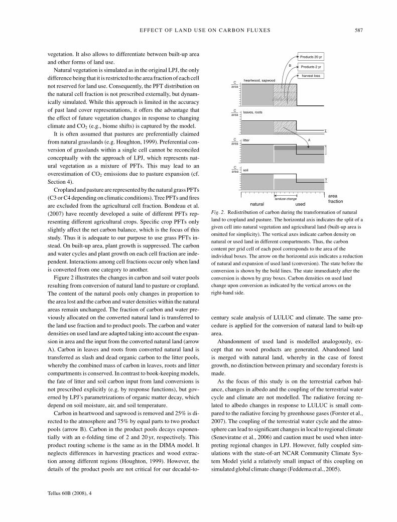
Figure 2 illustrates the changes in carbon and soil water poolsresulting from conversion of natural land to pasture or cropland.The content of the natural pools only changes in proportion tothe area lost and the carbon and water densities within the naturalareas remain unchanged. The fraction of carbon and water pre-viously allocated on the converted natural land is transferred tothe land use fraction and to product pools. The carbon and waterdensities on used land are adapted taking into account the expan-sion in area and the input from the converted natural land (arrowA). Carbon in leaves and roots from converted natural land istransferred as slash and dead organic carbon to the litter pools,whereby the combined mass of carbon in leaves, roots and littercompartments is conserved. In contrast to book-keeping models,the fate of litter and soil carbon input from land conversions isnot prescribed explicitly (e.g. by response functions), but gov-erned by LPJ’s parametrizations of organic matter decay, whichdepend on soil moisture, air, and soil temperature.
Carbon in heartwood and sapwood is removed and 25% is di-rected to the atmosphere and 75% by equal parts to two productpools (arrow B). Carbon in the product pools decays exponen-tially with an e-folding time of 2 and 20 yr, respectively. Thisproduct routing scheme is the same as in the DIMA model. Itneglects differences in harvesting practices and wood extrac-tion among different regions (Houghton, 1999). However, thedetails of the product pools are not critical for our decadal-to-
Fig. 2. Redistribution of carbon during the transformation of naturalland to cropland and pasture. The horizontal axis indicates the split of agiven cell into natural vegetation and agricultural land (built-up area isomitted for simplicity). The vertical axes indicate carbon density onnatural or used land in different compartments. Thus, the carboncontent per grid cell of each pool corresponds to the area of theindividual boxes. The arrow on the horizontal axis indicates a reductionof natural and expansion of used land (conversion). The state before theconversion is shown by the bold lines. The state immediately after theconversion is shown by gray boxes. Carbon densities on used landchange upon conversion as indicated by the vertical arrows on theright-hand side.
century scale analysis of LULUC and climate. The same pro-cedure is applied for the conversion of natural land to built-uparea.
Abandonment of used land is modelled analogously, ex-cept that no wood products are generated. Abandoned landis merged with natural land, whereby in the case of forestgrowth, no distinction between primary and secondary forests ismade.
As the focus of this study is on the terrestrial carbon bal-ance, changes in albedo and the coupling of the terrestrial watercycle and climate are not modelled. The radiative forcing re-lated to albedo changes in response to LULUC is small com-pared to the radiative forcing by greenhouse gases (Forster et al.,2007). The coupling of the terrestrial water cycle and the atmo-sphere can lead to significant changes in local to regional climate(Seneviratne et al., 2006) and caution must be used when inter-preting regional changes in LPJ. However, fully coupled sim-ulations with the state-of-art NCAR Community Climate Sys-tem Model yield a relatively small impact of this coupling onsimulated global climate change (Feddema et al., 2005).
Tellus 60B (2008), 4
588 K. M. STRASSMANN ET AL.
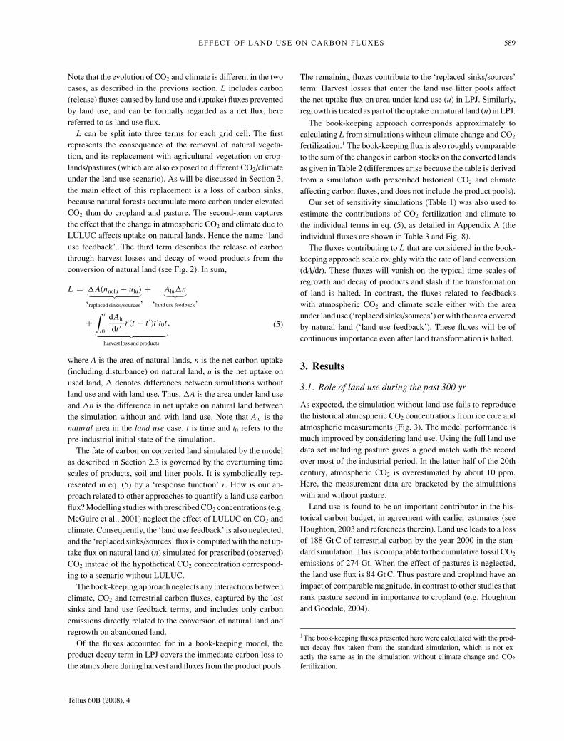
Table 1. Simulated net biospheric uptake in Gt C. Shown are integrated fluxes over the historical period, and the 21st century for scenario A2and A2 with land use area kept constant after 2000 A.D. (‘A2 commitment’). Results are for simulations with natural vegetation (‘no LU’),with prescribed pasture, cropland and built-up area (‘LU’), and with prescribed cropland and built-up area (‘no pasture’). Model settings areindicated in the first three columns. The simulations with simulated and prescribed CO2 yield identical results when both CO2 fertilization andclimate change are shut off (bottom row). Dashes indicate settings for which no simulation was performed
historical A2 A2 commitment1700–1999 2000–2099 2000–2099
Historical Climate CO2
CO2 change fertil. No LU LU . . . no pasture No LU LU . . . no pasture LU . . . no pasture
Simulated � � 73.3 −115.0 −10.4 264.9 53.5 153.2 114.6 208.8Simulated � × −5.0 −254.9 −118.1 −275.4 −326.2 −318.2 −282.9 −275.1Simulated × � 75.0 −101.4 −2.8 468.1 302.0 370.2 – –
Prescribed � � 126.7 −123.1 13.4 248.7 58.5 142.6 119.9 202.9Prescribed � × −14.9 −241.1 −116.3 −267.2 −320.7 −312.4 −276.5 −267.8Prescribed × � 139.6 −110.0 26.8 459.3 304.3 364.6 – –
Sim./presc. × × 2.6 −224.2 −100.5 0.1 −49.7 −44.5 – –
2.5. Simulation protocol and spin-up
In the standard setup, the BernCC model is forced with landcover data for cropland, pasture, and built-up area and emissionsof CO2 and of other radiative agents and precursor substances.Data-based emission estimates are used for the industrial period(Fuglestvedt and Berntsen, 1999; Joos et al., 2001) and projectedemissions for the IIASA A2, B1 and B2 scenarios.
For the assessment of the impact of land use on the carbon cy-cle, on CO2 and climate, simulations with land use are comparedto corresponding baseline simulations without land use.
A range of sensitivity simulations were performed to quan-tify the importance of individual processes on the impact of landuse on carbon fluxes and climate variables (Table 1 providesthe results for scenario A2; corresponding results for scenar-ios B1, B2 are given in Table 7). Many previous studies usingspatially explicit land use data considered only the evolution ofcropland (e.g. McGuire et al., 2001; Brovkin et al., 2004), but notchanges in pasture. Correspondingly, we ran ‘no pasture’ simula-tions considering only cropland and built-up area. Earlier studies(Joos et al., 2001; Gerber et al., 2004) identified the stimulationof carbon uptake by rising CO2 levels enhancing water use effi-ciency (CO2 fertilization) and the release of carbon in responseto heat stress and accelerated soil respiration under warming cli-mate as the dominant mechanisms governing changes in carbonstorage in LPJ-DGVM. In the ‘constant climate’ simulations,the climate sensitivity is set to zero and no long-term climatechange is simulated. In the ‘no CO2 fertilization’ simulations,CO2 is kept at its pre-industrial value in the LPJ-DGVM module.
Atmospheric CO2 would have evolved differently in the ab-sence of LULUC than observed. Different atmospheric CO2
concentration histories yield different evolutions of climate (inresponse to CO2 forcing) and of terrestrial carbon stocks (inresponse to CO2 fertilization and climate change). Thus, to beable to estimate the total earth system impact of LULUC, we
use a standard model setup where atmospheric CO2 is simulatedthroughout the whole simulated period. Consequently, the base-line simulation and the simulation with land use have differentCO2 concentrations and climate.
In addition, simulations have been performed with atmo-spheric CO2 before 2000 A.D. prescribed according to observa-tions (‘CO2 prescribed’). The historical part of these simulationsis compared with earlier studies using terrestrial models off-line(e.g. McGuire et al., 2001). The future part, on the other hand, isused to compare different scenarios of land use (with and with-out pasture) and emissions and land use change (A2, B1, B2)with a common starting point at the year 2000.
The inertia related to land use processes and the commitmentof past LULUC on future atmospheric CO2 and climate is quan-tified with simulations in which land use change is stalled at2000.
LPJ-DGVM is spun up from bare ground for 1000 yr underpre-industrial CO2, a baseline climate that includes interannualvariability (Leemans and Cramer, 1991; Cramer et al., 2001)and the land cover distribution for 1700 AD. At year 400, soilcarbon is set to the equilibrium value corresponding to currentlitter input and decomposition rates. The spin-up is continued foranother 600 yr to reach equilibrium. No spin-up is required forthe other BernCC model components. In transient simulations,the LPJ-DGVM module is forced by the boundary conditions asdescribed in Sections 2.3 and 2.4.
2.6. Land use flux analysis
The impact of LULUC on the terrestrial carbon cycle is assessedas the difference L in the net terrestrial uptake F between thesimulations without land use (nolu) and with land use (lu):
L = Fnolu − Flu. (4)
Tellus 60B (2008), 4
EFFECT OF LAND USE ON CARBON FLUXES 589
Note that the evolution of CO2 and climate is different in the twocases, as described in the previous section. L includes carbon(release) fluxes caused by land use and (uptake) fluxes preventedby land use, and can be formally regarded as a net flux, herereferred to as land use flux.
L can be split into three terms for each grid cell. The firstrepresents the consequence of the removal of natural vegeta-tion, and its replacement with agricultural vegetation on crop-lands/pastures (which are also exposed to different CO2/climateunder the land use scenario). As will be discussed in Section 3,the main effect of this replacement is a loss of carbon sinks,because natural forests accumulate more carbon under elevatedCO2 than do cropland and pasture. The second-term capturesthe effect that the change in atmospheric CO2 and climate due toLULUC affects uptake on natural lands. Hence the name ‘landuse feedback’. The third term describes the release of carbonthrough harvest losses and decay of wood products from theconversion of natural land (see Fig. 2). In sum,
L = �A(nnolu − ulu)︸ ︷︷ ︸‘replaced sinks/sources’
+ Alu�n︸ ︷︷ ︸‘land use feedback’
+∫ t
t0
dAlu
dt ′ r (t − t ′)t ′t0t︸ ︷︷ ︸
harvest loss and products
, (5)
where A is the area of natural lands, n is the net carbon uptake(including disturbance) on natural land, u is the net uptake onused land, � denotes differences between simulations withoutland use and with land use. Thus, �A is the area under land useand �n is the difference in net uptake on natural land betweenthe simulation without and with land use. Note that Alu is thenatural area in the land use case. t is time and t0 refers to thepre-industrial initial state of the simulation.
The fate of carbon on converted land simulated by the modelas described in Section 2.3 is governed by the overturning timescales of products, soil and litter pools. It is symbolically rep-resented in eq. (5) by a ‘response function’ r. How is our ap-proach related to other approaches to quantify a land use carbonflux? Modelling studies with prescribed CO2 concentrations (e.g.McGuire et al., 2001) neglect the effect of LULUC on CO2 andclimate. Consequently, the ‘land use feedback’ is also neglected,and the ‘replaced sinks/sources’ flux is computed with the net up-take flux on natural land (n) simulated for prescribed (observed)CO2 instead of the hypothetical CO2 concentration correspond-ing to a scenario without LULUC.
The book-keeping approach neglects any interactions betweenclimate, CO2 and terrestrial carbon fluxes, captured by the lostsinks and land use feedback terms, and includes only carbonemissions directly related to the conversion of natural land andregrowth on abandoned land.
Of the fluxes accounted for in a book-keeping model, theproduct decay term in LPJ covers the immediate carbon loss tothe atmosphere during harvest and fluxes from the product pools.
The remaining fluxes contribute to the ‘replaced sinks/sources’term: Harvest losses that enter the land use litter pools affectthe net uptake flux on area under land use (u) in LPJ. Similarly,regrowth is treated as part of the uptake on natural land (n) in LPJ.
The book-keeping approach corresponds approximately tocalculating L from simulations without climate change and CO2
fertilization.1 The book-keeping flux is also roughly comparableto the sum of the changes in carbon stocks on the converted landsas given in Table 2 (differences arise because the table is derivedfrom a simulation with prescribed historical CO2 and climateaffecting carbon fluxes, and does not include the product pools).
Our set of sensitivity simulations (Table 1) was also used toestimate the contributions of CO2 fertilization and climate tothe individual terms in eq. (5), as detailed in Appendix A (theindividual fluxes are shown in Table 3 and Fig. 8).
The fluxes contributing to L that are considered in the book-keeping approach scale roughly with the rate of land conversion(dA/dt). These fluxes will vanish on the typical time scales ofregrowth and decay of products and slash if the transformationof land is halted. In contrast, the fluxes related to feedbackswith atmospheric CO2 and climate scale either with the areaunder land use (‘replaced sinks/sources’) or with the area coveredby natural land (‘land use feedback’). These fluxes will be ofcontinuous importance even after land transformation is halted.
3. Results
3.1. Role of land use during the past 300 yr
As expected, the simulation without land use fails to reproducethe historical atmospheric CO2 concentrations from ice core andatmospheric measurements (Fig. 3). The model performance ismuch improved by considering land use. Using the full land usedata set including pasture gives a good match with the recordover most of the industrial period. In the latter half of the 20thcentury, atmospheric CO2 is overestimated by about 10 ppm.Here, the measurement data are bracketed by the simulationswith and without pasture.
Land use is found to be an important contributor in the his-torical carbon budget, in agreement with earlier estimates (seeHoughton, 2003 and references therein). Land use leads to a lossof 188 Gt C of terrestrial carbon by the year 2000 in the stan-dard simulation. This is comparable to the cumulative fossil CO2
emissions of 274 Gt. When the effect of pastures is neglected,the land use flux is 84 Gt C. Thus pasture and cropland have animpact of comparable magnitude, in contrast to other studies thatrank pasture second in importance to cropland (e.g. Houghtonand Goodale, 2004).
1The book-keeping fluxes presented here were calculated with the prod-uct decay flux taken from the standard simulation, which is not ex-actly the same as in the simulation without climate change and CO2
fertilization.
Tellus 60B (2008), 4
590 K. M. STRASSMANN ET AL.
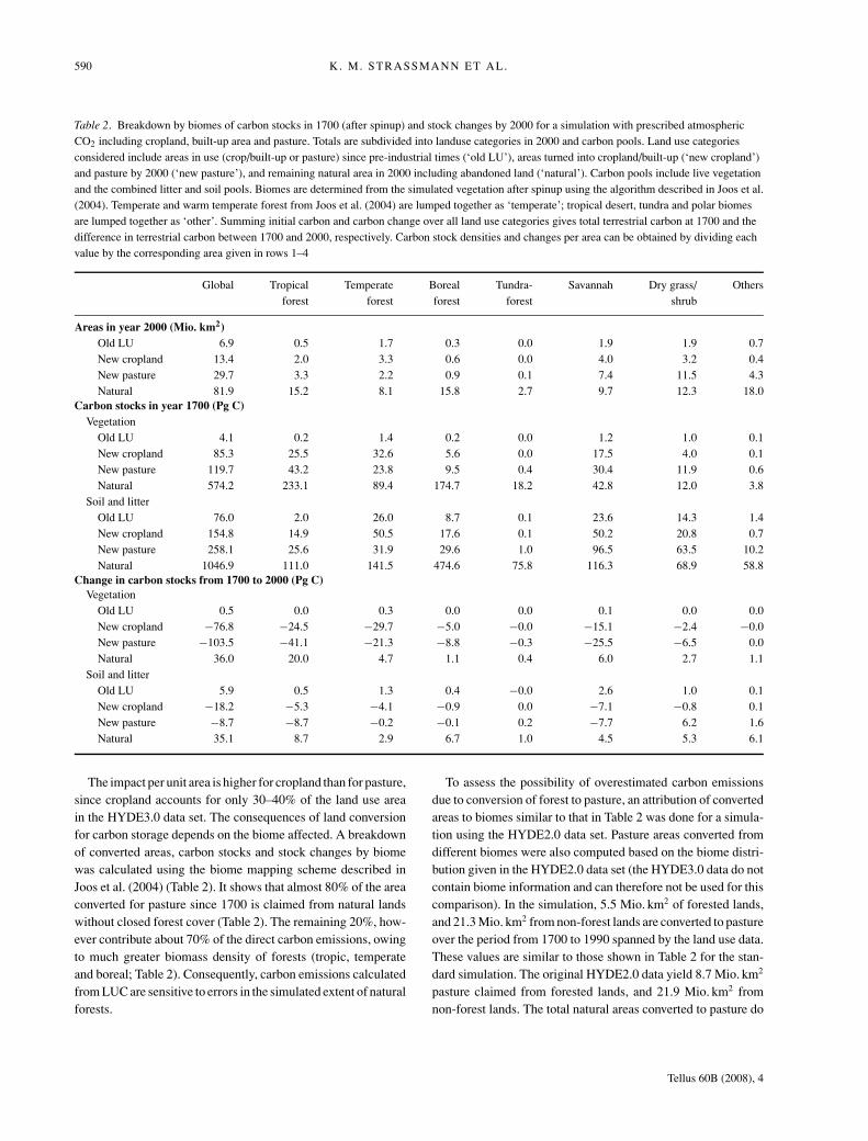
Table 2. Breakdown by biomes of carbon stocks in 1700 (after spinup) and stock changes by 2000 for a simulation with prescribed atmosphericCO2 including cropland, built-up area and pasture. Totals are subdivided into landuse categories in 2000 and carbon pools. Land use categoriesconsidered include areas in use (crop/built-up or pasture) since pre-industrial times (‘old LU’), areas turned into cropland/built-up (‘new cropland’)and pasture by 2000 (‘new pasture’), and remaining natural area in 2000 including abandoned land (‘natural’). Carbon pools include live vegetationand the combined litter and soil pools. Biomes are determined from the simulated vegetation after spinup using the algorithm described in Joos et al.(2004). Temperate and warm temperate forest from Joos et al. (2004) are lumped together as ‘temperate’; tropical desert, tundra and polar biomesare lumped together as ‘other’. Summing initial carbon and carbon change over all land use categories gives total terrestrial carbon at 1700 and thedifference in terrestrial carbon between 1700 and 2000, respectively. Carbon stock densities and changes per area can be obtained by dividing eachvalue by the corresponding area given in rows 1–4
Global Tropical Temperate Boreal Tundra- Savannah Dry grass/ Othersforest forest forest forest shrub
Areas in year 2000 (Mio. km2)
Old LU 6.9 0.5 1.7 0.3 0.0 1.9 1.9 0.7New cropland 13.4 2.0 3.3 0.6 0.0 4.0 3.2 0.4New pasture 29.7 3.3 2.2 0.9 0.1 7.4 11.5 4.3Natural 81.9 15.2 8.1 15.8 2.7 9.7 12.3 18.0
Carbon stocks in year 1700 (Pg C)
VegetationOld LU 4.1 0.2 1.4 0.2 0.0 1.2 1.0 0.1New cropland 85.3 25.5 32.6 5.6 0.0 17.5 4.0 0.1New pasture 119.7 43.2 23.8 9.5 0.4 30.4 11.9 0.6Natural 574.2 233.1 89.4 174.7 18.2 42.8 12.0 3.8
Soil and litterOld LU 76.0 2.0 26.0 8.7 0.1 23.6 14.3 1.4New cropland 154.8 14.9 50.5 17.6 0.1 50.2 20.8 0.7New pasture 258.1 25.6 31.9 29.6 1.0 96.5 63.5 10.2Natural 1046.9 111.0 141.5 474.6 75.8 116.3 68.9 58.8
Change in carbon stocks from 1700 to 2000 (Pg C)
VegetationOld LU 0.5 0.0 0.3 0.0 0.0 0.1 0.0 0.0New cropland −76.8 −24.5 −29.7 −5.0 −0.0 −15.1 −2.4 −0.0New pasture −103.5 −41.1 −21.3 −8.8 −0.3 −25.5 −6.5 0.0Natural 36.0 20.0 4.7 1.1 0.4 6.0 2.7 1.1
Soil and litterOld LU 5.9 0.5 1.3 0.4 −0.0 2.6 1.0 0.1New cropland −18.2 −5.3 −4.1 −0.9 0.0 −7.1 −0.8 0.1New pasture −8.7 −8.7 −0.2 −0.1 0.2 −7.7 6.2 1.6Natural 35.1 8.7 2.9 6.7 1.0 4.5 5.3 6.1
The impact per unit area is higher for cropland than for pasture,since cropland accounts for only 30–40% of the land use areain the HYDE3.0 data set. The consequences of land conversionfor carbon storage depends on the biome affected. A breakdownof converted areas, carbon stocks and stock changes by biomewas calculated using the biome mapping scheme described inJoos et al. (2004) (Table 2). It shows that almost 80% of the areaconverted for pasture since 1700 is claimed from natural landswithout closed forest cover (Table 2). The remaining 20%, how-ever contribute about 70% of the direct carbon emissions, owingto much greater biomass density of forests (tropic, temperateand boreal; Table 2). Consequently, carbon emissions calculatedfrom LUC are sensitive to errors in the simulated extent of naturalforests.
To assess the possibility of overestimated carbon emissionsdue to conversion of forest to pasture, an attribution of convertedareas to biomes similar to that in Table 2 was done for a simula-tion using the HYDE2.0 data set. Pasture areas converted fromdifferent biomes were also computed based on the biome distri-bution given in the HYDE2.0 data set (the HYDE3.0 data do notcontain biome information and can therefore not be used for thiscomparison). In the simulation, 5.5 Mio. km2 of forested lands,and 21.3 Mio. km2 from non-forest lands are converted to pastureover the period from 1700 to 1990 spanned by the land use data.These values are similar to those shown in Table 2 for the stan-dard simulation. The original HYDE2.0 data yield 8.7 Mio. km2
pasture claimed from forested lands, and 21.9 Mio. km2 fromnon-forest lands. The total natural areas converted to pasture do
Tellus 60B (2008), 4
EFFECT OF LAND USE ON CARBON FLUXES 591
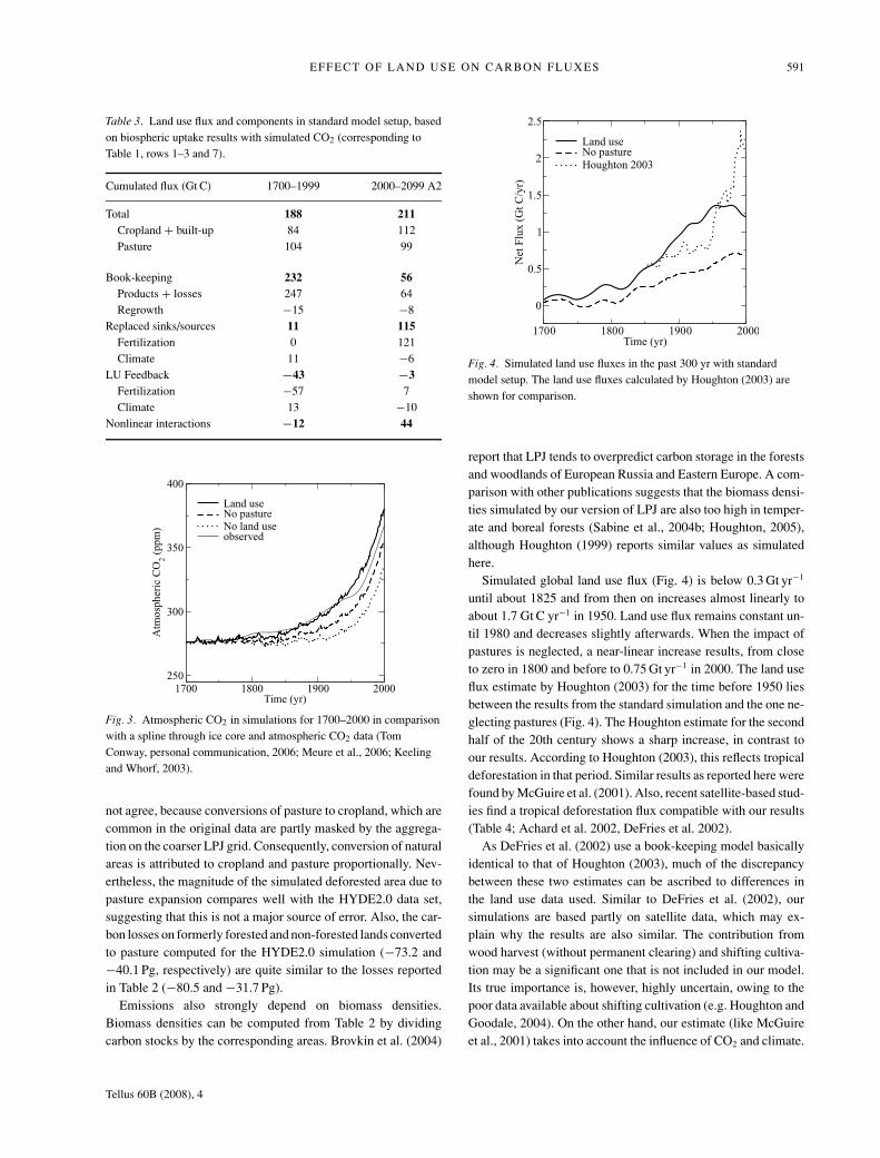
Table 3. Land use flux and components in standard model setup, basedon biospheric uptake results with simulated CO2 (corresponding toTable 1, rows 1–3 and 7).
Cumulated flux (Gt C) 1700–1999 2000–2099 A2
Total 188 211
Cropland + built-up 84 112Pasture 104 99
Book-keeping 232 56
Products + losses 247 64Regrowth −15 −8
Replaced sinks/sources 11 115
Fertilization 0 121Climate 11 −6
LU Feedback −43 −3
Fertilization −57 7Climate 13 −10
Nonlinear interactions −12 44
1700 1800 1900 2000Time (yr)
250
300
350
400
Atm
osp
her
ic C
O2 (
pp
m)
Land useNo pastureNo land useobserved
Fig. 3. Atmospheric CO2 in simulations for 1700–2000 in comparisonwith a spline through ice core and atmospheric CO2 data (TomConway, personal communication, 2006; Meure et al., 2006; Keelingand Whorf, 2003).
not agree, because conversions of pasture to cropland, which arecommon in the original data are partly masked by the aggrega-tion on the coarser LPJ grid. Consequently, conversion of naturalareas is attributed to cropland and pasture proportionally. Nev-ertheless, the magnitude of the simulated deforested area due topasture expansion compares well with the HYDE2.0 data set,suggesting that this is not a major source of error. Also, the car-bon losses on formerly forested and non-forested lands convertedto pasture computed for the HYDE2.0 simulation (−73.2 and−40.1 Pg, respectively) are quite similar to the losses reportedin Table 2 (−80.5 and −31.7 Pg).
Emissions also strongly depend on biomass densities.Biomass densities can be computed from Table 2 by dividingcarbon stocks by the corresponding areas. Brovkin et al. (2004)
1700 1800 1900 2000Time (yr)
0
0.5
1
1.5
2
2.5
Net
Flu
x (
Gt
C/y
r)
Land useNo pastureHoughton 2003
Fig. 4. Simulated land use fluxes in the past 300 yr with standardmodel setup. The land use fluxes calculated by Houghton (2003) areshown for comparison.
report that LPJ tends to overpredict carbon storage in the forestsand woodlands of European Russia and Eastern Europe. A com-parison with other publications suggests that the biomass densi-ties simulated by our version of LPJ are also too high in temper-ate and boreal forests (Sabine et al., 2004b; Houghton, 2005),although Houghton (1999) reports similar values as simulatedhere.
Simulated global land use flux (Fig. 4) is below 0.3 Gt yr−1
until about 1825 and from then on increases almost linearly toabout 1.7 Gt C yr−1 in 1950. Land use flux remains constant un-til 1980 and decreases slightly afterwards. When the impact ofpastures is neglected, a near-linear increase results, from closeto zero in 1800 and before to 0.75 Gt yr−1 in 2000. The land useflux estimate by Houghton (2003) for the time before 1950 liesbetween the results from the standard simulation and the one ne-glecting pastures (Fig. 4). The Houghton estimate for the secondhalf of the 20th century shows a sharp increase, in contrast toour results. According to Houghton (2003), this reflects tropicaldeforestation in that period. Similar results as reported here werefound by McGuire et al. (2001). Also, recent satellite-based stud-ies find a tropical deforestation flux compatible with our results(Table 4; Achard et al. 2002, DeFries et al. 2002).
As DeFries et al. (2002) use a book-keeping model basicallyidentical to that of Houghton (2003), much of the discrepancybetween these two estimates can be ascribed to differences inthe land use data used. Similar to DeFries et al. (2002), oursimulations are based partly on satellite data, which may ex-plain why the results are also similar. The contribution fromwood harvest (without permanent clearing) and shifting cultiva-tion may be a significant one that is not included in our model.Its true importance is, however, highly uncertain, owing to thepoor data available about shifting cultivation (e.g. Houghton andGoodale, 2004). On the other hand, our estimate (like McGuireet al., 2001) takes into account the influence of CO2 and climate.
Tellus 60B (2008), 4
592 K. M. STRASSMANN ET AL.
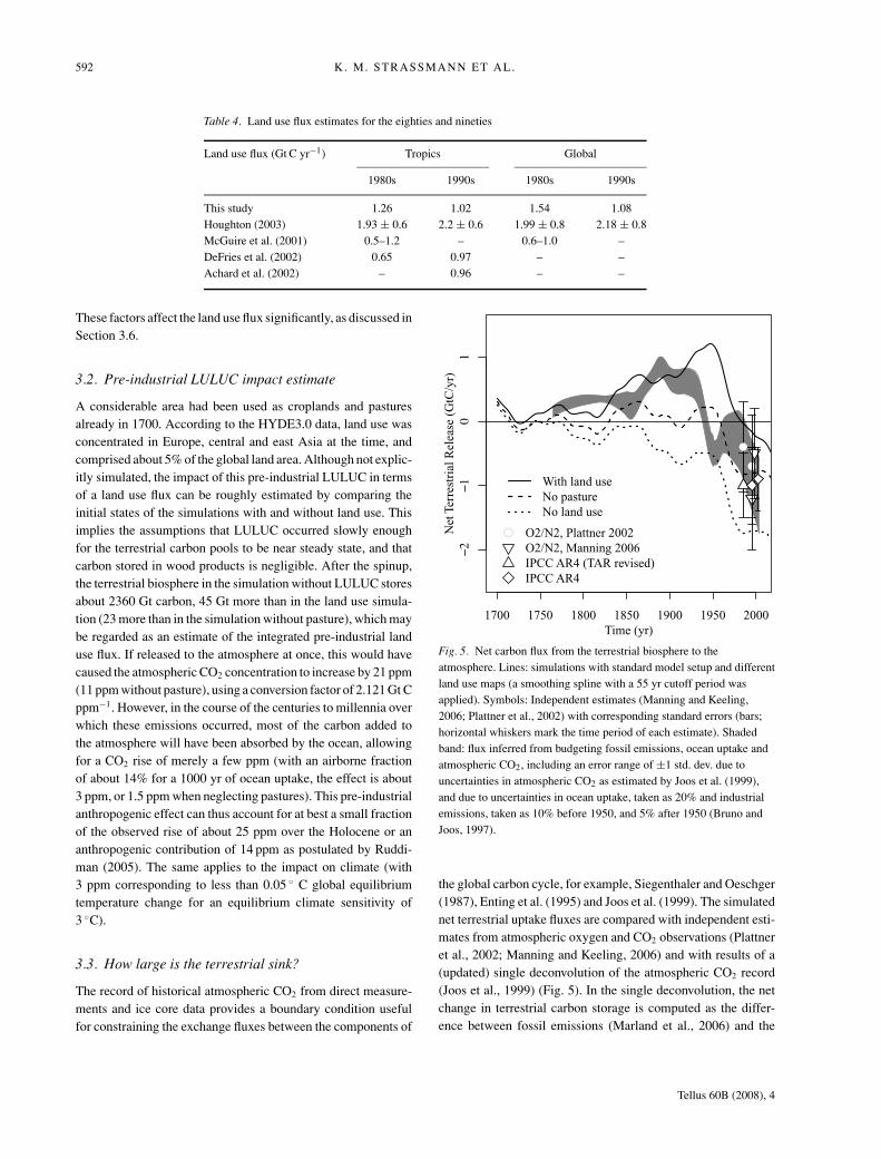
Table 4. Land use flux estimates for the eighties and nineties
Land use flux (Gt C yr−1) Tropics Global
1980s 1990s 1980s 1990s
This study 1.26 1.02 1.54 1.08Houghton (2003) 1.93 ± 0.6 2.2 ± 0.6 1.99 ± 0.8 2.18 ± 0.8McGuire et al. (2001) 0.5–1.2 – 0.6–1.0 –DeFries et al. (2002) 0.65 0.97 – –Achard et al. (2002) – 0.96 – –
These factors affect the land use flux significantly, as discussed inSection 3.6.
3.2. Pre-industrial LULUC impact estimate
A considerable area had been used as croplands and pasturesalready in 1700. According to the HYDE3.0 data, land use wasconcentrated in Europe, central and east Asia at the time, andcomprised about 5% of the global land area. Although not explic-itly simulated, the impact of this pre-industrial LULUC in termsof a land use flux can be roughly estimated by comparing theinitial states of the simulations with and without land use. Thisimplies the assumptions that LULUC occurred slowly enoughfor the terrestrial carbon pools to be near steady state, and thatcarbon stored in wood products is negligible. After the spinup,the terrestrial biosphere in the simulation without LULUC storesabout 2360 Gt carbon, 45 Gt more than in the land use simula-tion (23 more than in the simulation without pasture), which maybe regarded as an estimate of the integrated pre-industrial landuse flux. If released to the atmosphere at once, this would havecaused the atmospheric CO2 concentration to increase by 21 ppm(11 ppm without pasture), using a conversion factor of 2.121 Gt Cppm−1. However, in the course of the centuries to millennia overwhich these emissions occurred, most of the carbon added tothe atmosphere will have been absorbed by the ocean, allowingfor a CO2 rise of merely a few ppm (with an airborne fractionof about 14% for a 1000 yr of ocean uptake, the effect is about3 ppm, or 1.5 ppm when neglecting pastures). This pre-industrialanthropogenic effect can thus account for at best a small fractionof the observed rise of about 25 ppm over the Holocene or ananthropogenic contribution of 14 ppm as postulated by Ruddi-man (2005). The same applies to the impact on climate (with3 ppm corresponding to less than 0.05 ◦ C global equilibriumtemperature change for an equilibrium climate sensitivity of3 ◦C).
3.3. How large is the terrestrial sink?
The record of historical atmospheric CO2 from direct measure-ments and ice core data provides a boundary condition usefulfor constraining the exchange fluxes between the components of
1700 1750 1800 1850 1900 1950 2000Time (yr)
Net
Ter
rest
rial
Rel
ease
(G
tC/y
r)●
●
With land useNo pastureNo land use
● O2/N2, Plattner 2002O2/N2, Manning 2006IPCC AR4 (TAR revised)IPCC AR4
Fig. 5. Net carbon flux from the terrestrial biosphere to theatmosphere. Lines: simulations with standard model setup and differentland use maps (a smoothing spline with a 55 yr cutoff period wasapplied). Symbols: Independent estimates (Manning and Keeling,2006; Plattner et al., 2002) with corresponding standard errors (bars;horizontal whiskers mark the time period of each estimate). Shadedband: flux inferred from budgeting fossil emissions, ocean uptake andatmospheric CO2, including an error range of ±1 std. dev. due touncertainties in atmospheric CO2 as estimated by Joos et al. (1999),and due to uncertainties in ocean uptake, taken as 20% and industrialemissions, taken as 10% before 1950, and 5% after 1950 (Bruno andJoos, 1997).
the global carbon cycle, for example, Siegenthaler and Oeschger(1987), Enting et al. (1995) and Joos et al. (1999). The simulatednet terrestrial uptake fluxes are compared with independent esti-mates from atmospheric oxygen and CO2 observations (Plattneret al., 2002; Manning and Keeling, 2006) and with results of a(updated) single deconvolution of the atmospheric CO2 record(Joos et al., 1999) (Fig. 5). In the single deconvolution, the netchange in terrestrial carbon storage is computed as the differ-ence between fossil emissions (Marland et al., 2006) and the
Tellus 60B (2008), 4
EFFECT OF LAND USE ON CARBON FLUXES 593
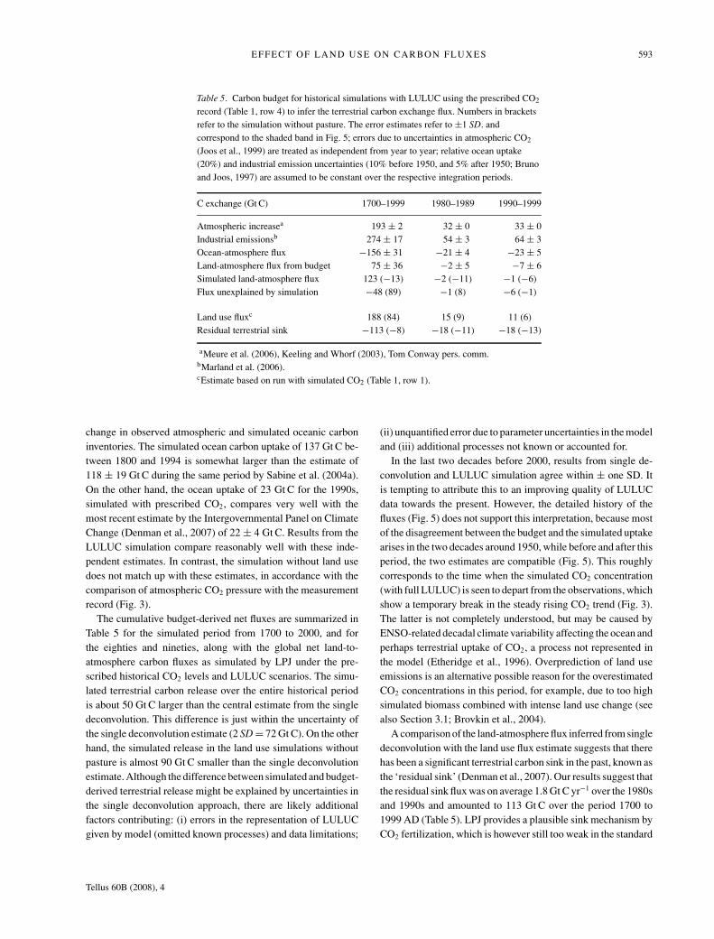
Table 5. Carbon budget for historical simulations with LULUC using the prescribed CO2
record (Table 1, row 4) to infer the terrestrial carbon exchange flux. Numbers in bracketsrefer to the simulation without pasture. The error estimates refer to ±1 SD. andcorrespond to the shaded band in Fig. 5; errors due to uncertainties in atmospheric CO2
(Joos et al., 1999) are treated as independent from year to year; relative ocean uptake(20%) and industrial emission uncertainties (10% before 1950, and 5% after 1950; Brunoand Joos, 1997) are assumed to be constant over the respective integration periods.
C exchange (Gt C) 1700–1999 1980–1989 1990–1999
Atmospheric increasea 193 ± 2 32 ± 0 33 ± 0Industrial emissionsb 274 ± 17 54 ± 3 64 ± 3Ocean-atmosphere flux −156 ± 31 −21 ± 4 −23 ± 5Land-atmosphere flux from budget 75 ± 36 −2 ± 5 −7 ± 6Simulated land-atmosphere flux 123 (−13) −2 (−11) −1 (−6)Flux unexplained by simulation −48 (89) −1 (8) −6 (−1)
Land use fluxc 188 (84) 15 (9) 11 (6)Residual terrestrial sink −113 (−8) −18 (−11) −18 (−13)
aMeure et al. (2006), Keeling and Whorf (2003), Tom Conway pers. comm.bMarland et al. (2006).cEstimate based on run with simulated CO2 (Table 1, row 1).
change in observed atmospheric and simulated oceanic carboninventories. The simulated ocean carbon uptake of 137 Gt C be-tween 1800 and 1994 is somewhat larger than the estimate of118 ± 19 Gt C during the same period by Sabine et al. (2004a).On the other hand, the ocean uptake of 23 Gt C for the 1990s,simulated with prescribed CO2, compares very well with themost recent estimate by the Intergovernmental Panel on ClimateChange (Denman et al., 2007) of 22 ± 4 Gt C. Results from theLULUC simulation compare reasonably well with these inde-pendent estimates. In contrast, the simulation without land usedoes not match up with these estimates, in accordance with thecomparison of atmospheric CO2 pressure with the measurementrecord (Fig. 3).
The cumulative budget-derived net fluxes are summarized inTable 5 for the simulated period from 1700 to 2000, and forthe eighties and nineties, along with the global net land-to-atmosphere carbon fluxes as simulated by LPJ under the pre-scribed historical CO2 levels and LULUC scenarios. The simu-lated terrestrial carbon release over the entire historical periodis about 50 Gt C larger than the central estimate from the singledeconvolution. This difference is just within the uncertainty ofthe single deconvolution estimate (2 SD = 72 Gt C). On the otherhand, the simulated release in the land use simulations withoutpasture is almost 90 Gt C smaller than the single deconvolutionestimate. Although the difference between simulated and budget-derived terrestrial release might be explained by uncertainties inthe single deconvolution approach, there are likely additionalfactors contributing: (i) errors in the representation of LULUCgiven by model (omitted known processes) and data limitations;
(ii) unquantified error due to parameter uncertainties in the modeland (iii) additional processes not known or accounted for.
In the last two decades before 2000, results from single de-convolution and LULUC simulation agree within ± one SD. Itis tempting to attribute this to an improving quality of LULUCdata towards the present. However, the detailed history of thefluxes (Fig. 5) does not support this interpretation, because mostof the disagreement between the budget and the simulated uptakearises in the two decades around 1950, while before and after thisperiod, the two estimates are compatible (Fig. 5). This roughlycorresponds to the time when the simulated CO2 concentration(with full LULUC) is seen to depart from the observations, whichshow a temporary break in the steady rising CO2 trend (Fig. 3).The latter is not completely understood, but may be caused byENSO-related decadal climate variability affecting the ocean andperhaps terrestrial uptake of CO2, a process not represented inthe model (Etheridge et al., 1996). Overprediction of land useemissions is an alternative possible reason for the overestimatedCO2 concentrations in this period, for example, due to too highsimulated biomass combined with intense land use change (seealso Section 3.1; Brovkin et al., 2004).
A comparison of the land-atmosphere flux inferred from singledeconvolution with the land use flux estimate suggests that therehas been a significant terrestrial carbon sink in the past, known asthe ‘residual sink’ (Denman et al., 2007). Our results suggest thatthe residual sink flux was on average 1.8 Gt C yr−1 over the 1980sand 1990s and amounted to 113 Gt C over the period 1700 to1999 AD (Table 5). LPJ provides a plausible sink mechanism byCO2 fertilization, which is however still too weak in the standard
Tellus 60B (2008), 4
594 K. M. STRASSMANN ET AL.
model setup to allow the model to closely reproduce the observedatmospheric CO2 concentrations.
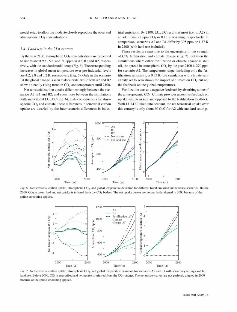
3.4. Land use in the 21st century
By the year 2100, atmospheric CO2 concentrations are projectedto rise to about 990, 590 and 710 ppm in A2, B1 and B2, respec-tively, with the standard model setup (Fig. 6). The correspondingincreases in global mean temperature over pre-industrial levelsare 4.2, 2.8 and 3.2 K, respectively (Fig. 6). Only in the scenarioB1 the global change is seen to decelerate, while both A2 and B2show a steadily rising trend in CO2 and temperature until 2100.
Net terrestrial carbon uptake differs strongly between the sce-narios A2, B1 and B2, and even more between the simulationswith and without LULUC (Fig. 6). In its consequences for atmo-spheric CO2 and climate, these differences in terrestrial carbonuptake are dwarfed by the inter-scenario differences in indus-
Fig. 6. Net terrestrial carbon uptake, atmospheric CO2, and global temperature deviation for different fossil emission and land use scenarios. Before2000, CO2 is prescribed and net uptake is inferred from the CO2 budget. The net uptake curves are not perfectly aligned in 2000 because of thespline smoothing applied.
Fig. 7. Net terrestrial carbon uptake, atmospheric CO2, and global temperature deviation for scenarios A2 and B1 with sensitivity settings and fullland use. Before 2000, CO2 is prescribed and net uptake is inferred from the CO2 budget. The net uptake curves are not perfectly aligned in 2000because of the spline smoothing applied.
trial emissions. By 2100, LULUC results at most (i.e. in A2) inan additional 72 ppm CO2 or 0.18 K warming, respectively. Incomparison, scenarios A2 and B1 differ by 395 ppm or 1.37 Kin 2100 (with land use included).
These results are sensitive to the uncertainty in the strengthof CO2 fertilization and climate change (Fig. 7). Between thesimulations where either fertilization or climate change is shutoff, the spread in atmospheric CO2 by the year 2100 is 270 ppmfor scenario A2. The temperature range, including only the fer-tilization sensitivity, is 0.33 K (the simulation with climate sen-sitivity set to zero shows the impact of climate on CO2 but notthe feedback on the global temperature).
Fertilization acts as a negative feedback by absorbing some ofthe anthropogenic CO2. Climate provides a positive feedback onuptake similar in size and opposed to the fertilization feedback.With LULUC taken into account, the net terrestrial uptake overthis century is only about 60 Gt C for A2 with standard settings.
Tellus 60B (2008), 4
EFFECT OF LAND USE ON CARBON FLUXES 595
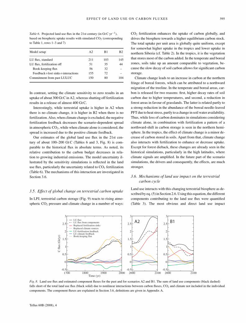
Table 6. Projected land use flux in the 21st century (in Gt C yr−1),based on biospheric uptake results with simulated CO2 (correspondingto Table 1, rows 1–3 and 7)
Model setup A2 B1 B2
LU flux, standard 211 103 145LU flux, fertilization off 51 35 44
Book-keeping flux 56 32 –Feedback+lost sinks+interactions 155 72 –
Commitment from past LULUC 150 80 104
In contrast, setting the climate sensitivity to zero results in anuptake of about 300 Gt C in A2, whereas shutting off fertilizationresults in a release of almost 400 Gt C.
Interestingly, while terrestrial uptake is higher in A2 whenthere is no climate change, it is higher in B2 when there is nofertilization. Also, when climate change is excluded, the negativefertilization feedback decreases the scenario-dependent spreadin atmospheric CO2, while when climate alone is considered, thespread is increased due to the positive climate feedback.
Our estimates of the global land use flux in the 21st cen-tury of about 100–200 Gt C (Tables 6 and 3, Fig. 8) is com-parable to the historical flux in absolute terms. As noted, itsrelative contribution to the carbon budget decreases in rela-tion to growing industrial emissions. The model uncertainty il-lustrated by the sensitivity simulations is reflected in the landuse flux, particularly the uncertainty related to CO2 fertilization(Table 6). The mechanisms of this interaction are investigated inSection 3.6.
3.5. Effect of global change on terrestrial carbon uptake
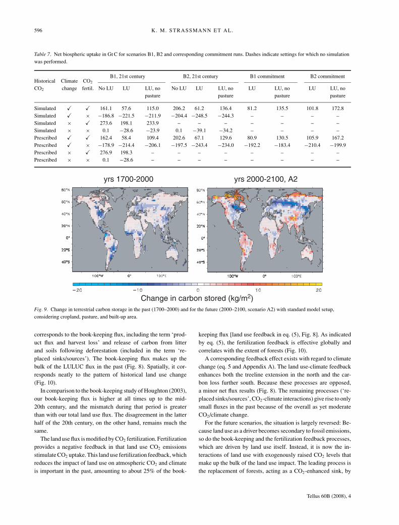
In LPJ, terrestrial carbon storage (Fig. 9) reacts to rising atmo-spheric CO2 pressure and climate change in a number of ways:
Fig. 8. Land use flux and estimated component fluxes for the past and for scenarios A2 and B1. The sum of land use components (black dashed)falls short of the total land use flux (black solid) due to nonlinear interactions between carbon fluxes, CO2 and climate not included in the individualcomponents. The component fluxes are explained in Section 3.6, definitions are given in Appendix A.
CO2 fertilization enhances the uptake of carbon globally, anddrives the biosphere towards a higher equilibrium carbon stock.The total uptake per unit area is globally quite uniform, exceptfor somewhat higher uptake in the tropics and lower uptake innorthern Siberia (cf. Table 2). In the tropics, it is the vegetationthat stores most of the carbon added. In the temperate and borealzones, soils take up an amount comparable to vegetation, be-cause the slow decay of soil carbon allows for significant carbonstorage.
Climate change leads to an increase in carbon at the northernfringe of boreal forests, which can be attributed to a northwardmigration of the treeline. In the temperate and boreal areas, car-bon is released for two reasons: first, higher decay rates of soilcarbon due to higher temperatures, and second, a reduction inforest areas in favour of grasslands. The latter is related partly toa strong reduction in the abundance of the boreal needle-leavedPFT due to heat stress, partly to a change in soil water availability.Thus, while loss of carbon dominates in simulations consideringclimate alone, in combination with fertilization a pattern of anorthward-shift in carbon storage is seen in the northern hemi-sphere. In the tropics, the effect of climate change is a minor de-crease of carbon stored in soils. Apart from that, climate changealso interacts with fertilization to enhance or decrease uptake.Except for forest dieback, these changes are already seen in thehistorical simulations, particularly in the high latitudes, whereclimate signals are amplified. In the future part of the scenariosimulations, the drivers and consequently, the effects, are muchstronger.
3.6. Mechanisms of land use impact on the terrestrialcarbon cycle
Land use interacts with this changing terrestrial biosphere as de-scribed by eq. (5) in Section 2.6. Using this equation, the differentcomponents contributing to the land use flux were quantified(Table 3). The most obvious and direct land use impact
Tellus 60B (2008), 4
596 K. M. STRASSMANN ET AL.
Table 7. Net biospheric uptake in Gt C for scenarios B1, B2 and corresponding commitment runs. Dashes indicate settings for which no simulationwas performed.
B1, 21st century B2, 21st century B1 commitment B2 commitmentHistorical Climate CO2
CO2 change fertil. No LU LU LU, no No LU LU LU, no LU LU, no LU LU, nopasture pasture pasture pasture
Simulated � � 161.1 57.6 115.0 206.2 61.2 136.4 81.2 135.5 101.8 172.8Simulated � × −186.8 −221.5 −211.9 −204.4 −248.5 −244.3 – – – –Simulated × � 273.6 198.1 233.9 – – – – – – –Simulated × × 0.1 −28.6 −23.9 0.1 −39.1 −34.2 – – – –Prescribed � � 162.4 58.4 109.4 202.6 67.1 129.6 80.9 130.5 105.9 167.2Prescribed � × −178.9 −214.4 −206.1 −197.5 −243.4 −234.0 −192.2 −183.4 −210.4 −199.9Prescribed × � 276.9 198.3 – – – – – – – –Prescribed × × 0.1 −28.6 – – – – – – – –
Fig. 9. Change in terrestrial carbon storage in the past (1700–2000) and for the future (2000–2100, scenario A2) with standard model setup,considering cropland, pasture, and built-up area.
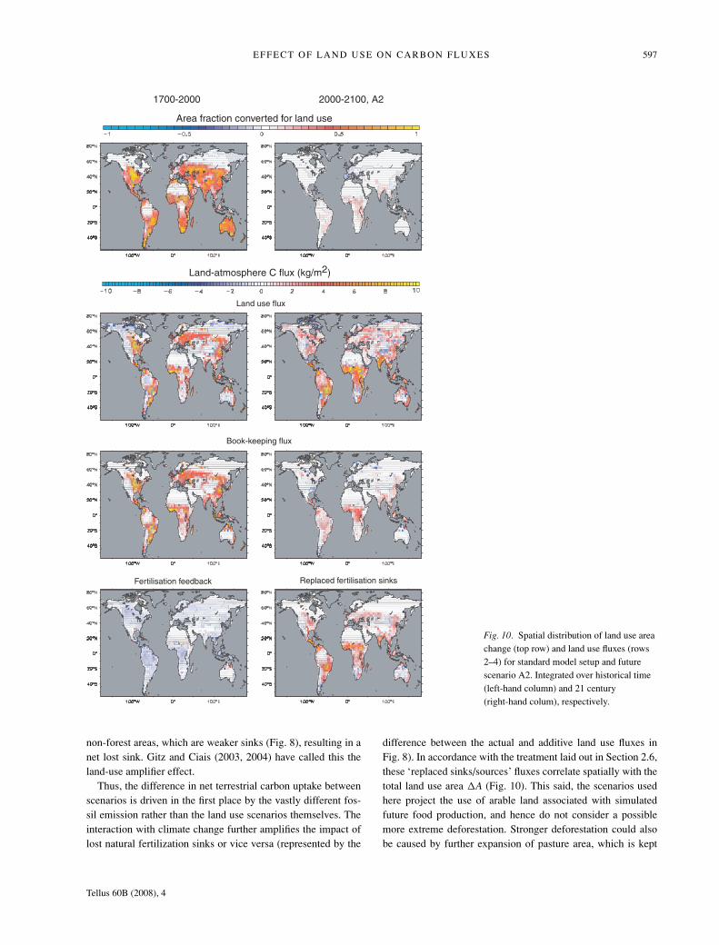
corresponds to the book-keeping flux, including the term ‘prod-uct flux and harvest loss’ and release of carbon from litterand soils following deforestation (included in the term ‘re-placed sinks/sources’). The book-keeping flux makes up thebulk of the LULUC flux in the past (Fig. 8). Spatially, it cor-responds neatly to the pattern of historical land use change(Fig. 10).
In comparison to the book-keeping study of Houghton (2003),our book-keeping flux is higher at all times up to the mid-20th century, and the mismatch during that period is greaterthan with our total land use flux. The disagreement in the latterhalf of the 20th century, on the other hand, remains much thesame.
The land use flux is modified by CO2 fertilization. Fertilizationprovides a negative feedback in that land use CO2 emissionsstimulate CO2 uptake. This land use fertilization feedback, whichreduces the impact of land use on atmospheric CO2 and climateis important in the past, amounting to about 25% of the book-
keeping flux [land use feedback in eq. (5), Fig. 8]. As indicatedby eq. (5), the fertilization feedback is effective globally andcorrelates with the extent of forests (Fig. 10).
A corresponding feedback effect exists with regard to climatechange (eq. 5 and Appendix A). The land use-climate feedbackenhances both the treeline extension in the north and the car-bon loss further south. Because these processes are opposed,a minor net flux results (Fig. 8). The remaining processes (‘re-placed sinks/sources’, CO2-climate interactions) give rise to onlysmall fluxes in the past because of the overall as yet moderateCO2/climate change.
For the future scenarios, the situation is largely reversed: Be-cause land use as a driver becomes secondary to fossil emissions,so do the book-keeping and the fertilization feedback processes,which are driven by land use itself. Instead, it is now the in-teractions of land use with exogenously raised CO2 levels thatmake up the bulk of the land use impact. The leading process isthe replacement of forests, acting as a CO2-enhanced sink, by
Tellus 60B (2008), 4
EFFECT OF LAND USE ON CARBON FLUXES 597
Fig. 10. Spatial distribution of land use areachange (top row) and land use fluxes (rows2–4) for standard model setup and futurescenario A2. Integrated over historical time(left-hand column) and 21 century(right-hand colum), respectively.
non-forest areas, which are weaker sinks (Fig. 8), resulting in anet lost sink. Gitz and Ciais (2003, 2004) have called this theland-use amplifier effect.
Thus, the difference in net terrestrial carbon uptake betweenscenarios is driven in the first place by the vastly different fos-sil emission rather than the land use scenarios themselves. Theinteraction with climate change further amplifies the impact oflost natural fertilization sinks or vice versa (represented by the
difference between the actual and additive land use fluxes inFig. 8). In accordance with the treatment laid out in Section 2.6,these ‘replaced sinks/sources’ fluxes correlate spatially with thetotal land use area �A (Fig. 10). This said, the scenarios usedhere project the use of arable land associated with simulatedfuture food production, and hence do not consider a possiblemore extreme deforestation. Stronger deforestation could alsobe caused by further expansion of pasture area, which is kept
Tellus 60B (2008), 4
598 K. M. STRASSMANN ET AL.
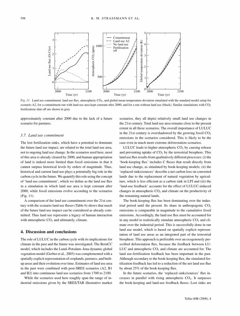
Fig. 11. Land use commitment: land use flux, atmospheric CO2, and global mean temperature deviation simulated with the standard model setup forscenario A2, for a commitment run with land use area kept constant after 2000, and for a run without land use (black). Similar simulations with CO2
fertilization shut off are shown in grey.
approximately constant after 2000 due to the lack of a futurescenario for pastures.
3.7. Land use commitment
The lost fertilization sinks, which have a potential to dominatethe future land use impact, are related to the total land use area,not to ongoing land use change. In the scenarios used here, mostof this area is already cleared by 2000, and human appropriationof land is indeed more limited than fossil emissions in that itcannot surpass historical levels by orders of magnitude. Thus,historical and current land use plays a potentially big role in thecarbon cycle in the future. We quantify this role using the conceptof ‘land use commitment’, which we define as the land use fluxin a simulation in which land use area is kept constant after2000, while fossil emissions evolve according to the scenarios(Fig. 11).
A comparison of the land use commitment over the 21st cen-tury with the scenario land use fluxes (Table 6) shows that muchof the future land use impact can be considered as already com-mitted. Thus land use represents a legacy of human interactionwith atmospheric CO2 and ultimately, climate.
4. Discussion and conclusions
The role of LULUC in the carbon cycle with its implications forclimate in the past and the future was investigated. The BernCCmodel, which includes the Lund–Potsdam–Jena dynamic globalvegetation model (Gerber et al., 2003) was complemented with aspatially explicit representation of croplands, pastures, and built-up areas and their evolution over time. Estimates of land use areain the past were combined with post-SRES scenarios (A2, B1and B2) into continuous land use scenarios from 1700 to 2100.
While the scenarios used here roughly span the range of in-dustrial emissions given by the SRES/TAR illustrative marker
scenarios, they all depict relatively small land use changes inthe 21st century. Total land use area remains close to the presentextent in all these scenarios. The overall importance of LULUCin the 21st century is overshadowed by the growing fossil CO2
emissions in the scenarios considered. This is likely to be thecase even in much more extreme deforestation scenarios.
LULUC leads to higher atmospheric CO2 by causing releaseand preventing uptake of CO2 by the terrestrial biosphere. Thisland use flux results from qualitatively different processes: (i) the‘book-keeping flux’ includes C fluxes that result directly fromland use change, as simulated by book-keeping models; (ii) the‘replaced sinks/sources’ describe a net carbon loss on convertedlands due to the replacement of natural vegetation by agricul-ture, which is less efficient as a carbon sink in LPJ and (iii) the‘land-use feedback’ accounts for the effect of LULUC-inducedchanges in atmospheric CO2 and climate on the productivity ofthe remaining natural lands.
The book-keeping flux has been dominating over the indus-trial period until the present. Its share in anthropogenic CO2
emissions is comparable in magnitude to the cumulative fossilemissions. Accordingly, the land use flux must be accounted forin any model to realistically simulate atmospheric CO2 and cli-mate over the industrial period. This is successfully done in ourland use model, which is based on spatially explicit represen-tation of land use areas as an integrated part of the terrestrialbiosphere. This approach is preferable over an exogenously pre-scribed deforestation flux, because the feedback between LU-LUC and atmospheric CO2 and climate are accounted for. Theland use-fertilization feedback has been important in the past.Although secondary to the book-keeping flux, the simulated fer-tilization feedback has led to a reduction of the net land use fluxby about 25% of the book-keeping flux.
In the future scenarios, the ‘replaced sinks/sources’ flux in-creases in parallel with rising atmospheric CO2. It surpassesthe book-keeping and land-use feedback fluxes. Lost sinks are
Tellus 60B (2008), 4
EFFECT OF LAND USE ON CARBON FLUXES 599
essentially the areas under land use. In the scenarios usedhere, most of the area under land use by 2100 is already con-verted today. Consequently, there is a commitment to future cli-mate change due to past LULUC. Possible scenarios featuringmore extreme deforestation scenarios would imply higher book-keeping fluxes. However, as more deforestation would also meanmore natural carbon sinks lost and higher CO2, the commitmentflux is likely to remain dominant in a large range of conceivablescenarios. Thus the conclusion is robust in that respect that mostof the future LULUC land use flux is due to a commitment frompast land use change.
The importance of the land use commitment leads us to de-emphasize the traditional book-keeping flux when consideringthe role of LULUC in the future. This conclusion hinges onthe magnitude of productivity stimulation by elevated CO2, andother factors not explicitly considered here, such as nitrogen de-position. A similar commitment effect could arise from differentsoil overturning rates on agricultural versus natural land. Theeffectiveness of these mechanisms and of CO2 fertilization inparticular in real ecosystems and under much higher CO2 levelsis still very unclear. Therefore, to understand the role of LULUC,we need to understand fertilization mechanisms.
The global carbon budget suggests a strong residual sink,which is commonly attributed to the terrestrial biosphere. In themodel, CO2 fertilization provides such a terrestrial sink, which isrequired to realistically reproduce historic CO2 concentrations.This sink is indeed still too weak to match the residual sink in-ferred from the global carbon budget. On the other hand, thismismatch could equally well be due to the omission or misrep-resentation of another process, whether related to land use or not.Our land use model omits forestry as well as other managementpractices, which are partly accounted for in Houghton (2003).However, Houghton and Goodale (2004) argues that these are ofsecondary importance in comparison to cropland and pasture ex-pansion. The role of shifting cultivation and forest degradationis potentially more important (Houghton and Goodale, 2004),but is hardly quantifiable for lack of reliable data. In light of thisuncertainty, we see the ‘first-order approach’ of including onlythe reasonably quantifiable and important effects justified.
In contrast to most previous studies, the newly availableHYDE3.0 data allowed us to take pastures into account, at leastfor the past and to some extent into the future. Although theland use flux per unit area from pastures is on average smallerthan that of cropland, due to the larger spatial extent of pastures,both cropland and pasture are of similar importance. In contrast,Houghton and Goodale (2004) rank LULUC for pasture sec-ondary in importance to cropland with a carbon source a thirdthe size of the latter. Apart from the latter half of 20th century, ourbook-keeping flux estimates are higher than those by Houghton(2003), which also include pasture. Part of this discrepancy mostlikely stems from the input data; a discussion of their limitationsis beyond the scope of this paper. But a significant remaining
difference may be due to the way land conversion for pasture ismodelled.
Deviations between simulated and actual vegetation distribu-tion are one source of error. However, the distribution of pastureareas claimed from forested vs. non-forested biomes in a simula-tion using the HYDE2.0 data is similar to that obtained from thebiome distribution given in the original HYDE2.0 data set. Thisresult does not suggest major errors to arise from the simulatedvegetation distribution. Another possibility is that pasture expan-sion does not affect the natural vegetation as strongly as assumedhere. Houghton (1999), e.g., assumes that pastures are claimedfrom natural grassland in North America and China, withoutaffecting carbon storage. For comparison, we estimate lossesin total carbon due to pasture expansion on savannah and drygrass/shrub lands of 34 Gt C worldwide (Table 2). A third possi-bility is overprediction of biomass per area. Brovkin et al. (2004)relate overprediction of CO2 emissions to cropland changes inthe 1950s in temperate regions with too high simulated carbonstocks. A similar effect might contribute to the overestimate ofCO2 seen here (Fig. 3), although in the HYDE3.0 data the tim-ing and spatial distribution of LUC does not show such a clearpattern as in the data of Ramankutty and Foley (1999) used byBrovkin et al. (2004). Data on carbon stocks of different biomeshave large uncertainties (Houghton, 1999; Sabine et al., 2004b;Houghton, 2005). The recent assessment by Sabine et al. (2004b)suggests that LPJ strongly overpredicts carbon storage in borealforests, and underpredicts soil carbon storage in tropical forests.Boreal forests only contribute about 15 Gt C to the total sim-ulated emissions of about 200 Gt C (Table 2). Emissions fromtropical soils might be some 20 Gt higher than the estimated14 Gt found here (Table 2). In conclusion, the global land useflux is not strongly biased by any one of these sources of error.
This study does not account for biogeophysical effects ofLULUC, as described by Sitch et al. (2005), Brovkin et al.(2004). The leading biogeophysical effect of LULUC arises fromthe strong difference in albedo between snow-covered forestsand grassland. Although there is considerable uncertainty in thequantification of this albedo difference in state-of-the-art climatemodels (Roesch, 2006), it should be noted that the LULUC-related albedo change results in a cooling effect opposed to andpotentially compensating or even overcompensating the radia-tive forcing of the land use CO2 flux (Bala et al., 2007).
Ruddiman (2005) presents an update of his ‘anthropogenic hy-pothesis’, according to which land use caused the atmosphericCO2 increase of about 14 ppm over the past 11 kyr. This anthro-pogenic CO2 rise is supposed to have prevented a cooling ofthe global climate and the onset of a new ice age. Based on theHYDE land use map for 1700 we estimate the potential impactof LULUC on atmospheric CO2 in pre-industrial times to a fewppm—much less than the postulated 14 ppm. Accordingly, thepotential impact of pre-industrial anthropogenic emissions onclimate is negligibly small.
Tellus 60B (2008), 4
600 K. M. STRASSMANN ET AL.
5. Acknowledgments
This work was funded by the International Institute of AppliedSystem Analysis, Vienna, in the framework of the Global Green-house Initiative and the Gains-Asia programs. We would like tothank the scientists from IIASA who have contributed to thiswork with helpful comments and discussions. We are also in-debted to Gian-Kasper Plattner, whose suggestions and criticalremarks helped improve this manuscript. Special thanks are dueto Kees Klein Goldewijk for providing the HYDE3.0 data set aswell as helpful and encouraging comments to the study.
6. Appendix A: Land use components
The deviation of the net terrestrial uptake from initial equilib-rium can be separated approximately into the effects of CO2,climate, and a remainder including in our model harvest lossesand regrowth terms (fluctuations are neglected).
n = nCO2 + nClim + nregrowth (A1)
u = uCO2 + uClim + uharvest loss, (A2)
where n and u are the net terrestrial uptake on natural and usedlands, respectively. These terms are quantified using sensitivitysimulations where climate sensitivity is zero (s0), or alterna-tively, fertilization is shut off (f0). The biospheric uptake termsappearing in eq. (5) are estimated as
nnolu � (ns0
nolu − ns0, f 0nolu
)︸ ︷︷ ︸
CO2
+ (n f 0
nolu − ns0, f 0nolu
)︸ ︷︷ ︸
Clim
+ ns0, f 0nolu︸ ︷︷ ︸�0
(A3)
ulu � (us0
lu − us0, f 0lu
)︸ ︷︷ ︸
CO2
+ (u f 0
lu − us0, f 0lu
)︸ ︷︷ ︸
Clim
+ us0, f 0lu︸ ︷︷ ︸
harvest loss
(A4)
�n � (ns0
nolu − ns0, f 0nolu
) − (ns0
lu − ns0, f 0lu
)︸ ︷︷ ︸
CO2
+ (n f 0
nolu − ns0, f 0nolu
) − (n f 0
lu − ns0, f 0lu
)︸ ︷︷ ︸
Clim
+ ns0, f 0nolu − ns0, f 0
lu︸ ︷︷ ︸regrowth
. (A5)
Expanding eq. (5) to use these approximations yields
L =i. Replaced fertilization sinks
ii. Replaced climate sinks/sourcesiii. Land use-fertilization feedbackiv. Land use-climate feedbackv. Book-keeping flux
vi. Interaction terms
(A6)
=i. �A
((ns0
nolu − ns0 f 0nolu
) − (us0
lu − us0 f 0lu
))+ii. �A
((n f 0
nolu − ns0 f 0nolu
) − (u f 0
lu − us0 f 0lu
))+iii. Alu
((ns0
nolu − ns0 f 0nolu
) − (ns0
lu − ns0 f 0lu
))+iv. Alu
((n f 0
nolu − ns0 f 0nolu
) − (n f 0
lu − ns0 f 0lu
))+v. �A
(ns0 f 0
nolu − us0 f 0lu
) + Alu
(ns0 f 0
nolu − ns0 f 0lu
) + P
vi.
⎧⎪⎪⎪⎪⎪⎨⎪⎪⎪⎪⎪⎩
+�A[(
nnolu + ns0 f 0nolu
) − (ns0
nolu + n f 0nolu
)−(
ulu + us0 f 0lu
) + (us0
lu + u f 0lu
)]+Alu
[(nnolu − nlu
) + (ns0 f 0
nolu − ns0 f 0lu
)−(
ns0nolu − ns0
lu
) − (n f 0
nolu − n f 0lu
)], (A7)
where P is the product decay flux, n is net uptake in the actualsimulation, L is the land use flux derived from the standard sim-ulations including all effects, the sum of terms i-v is the land useflux assuming additive effects of CO2 and climate, and term virepresents the interaction between the two. In the calculationspresented, built-up area is accounted for separately. It constitutesa minor contribution and is neglected here for simplicity.
7. Appendix B: Light competition scheme
In LPJ, competition for light is based on the fractional plant cover(FPC) of each plant functional type (PFT), and the constraintthat the sum of FPCs cannot exceed unity. This means that themaximum cross section on which light is absorbed is equal tothe surface area of the grid cell. Increase of FPC in excess ofthis limit is corrected for by shading mortality. The distributionof shading mortality among the PFTs present in a given grid celldetermines how light competition works.
In the Sitch et al. (2003) version of LPJ, shading mortality ‘ispartitioned among woody PFTs in proportion to the FPC incre-ment resulting from their biomass increment for this year.’ Thisbiomass increase is determined by the subroutine calculatingNPP. If this were the only process affecting FPC, this algorithmwould exactly cancel the growth of each PFT in excess of theavailable area. Consequently, in a cell in which FPC is at its max-imal value in a given year, any change to distribution of FPC perPFT would be cancelled, so that the cell would maintain its cur-rent distribution indefinitely, unless any of the PFTs are affectedby other processes like growing conditions turning worse due toclimate change. In effect, competition would be limited to theprimary establishment of vegetation from bare ground.
However, in LPJ, FPC is also changed when new plant indi-viduals are established, due to the added biomass of saplings.Establishment typically happens on a yearly basis. This has twoimplications. First, as the correction applied to each PFT doesnot exactly correspond to that PFTs status, the number of plantsof the given PFT to be removed can at times exceed the numberpresent. This must be corrected for to avoid negative plant densi-ties. Second, competition is strongly enhanced. In particular, the
Tellus 60B (2008), 4
EFFECT OF LAND USE ON CARBON FLUXES 601
tropical broad-leaved evergreen PFT gets a strong competitiveadvantage, allowing it under certain circumstances to displaceall other PFTs.
For the present study, the partitioning of shading mortalitywas changed: shading is partitioned in proportion to the totalFPC of each PFT, as opposed to the FPC increment. This ap-proach avoids the aforementioned problems while allowing forreasonable competition among PFTs.
References
Achard, F., Eva, H. D., Stibig, H. J., Mayaux, P., Gallego, J. and co-authors. 2002. Determination of deforestation rates of the world’shumid tropical forests. Science 297, 999–1002.
Bala, G., Caldeira, K., Wickett, M., Phillips, T. J., Lobell, D. B. and co-authors. 2007. Combined climate and carbon-cycle effects of large-scale deforestation. Proc. Natl. Acad. Sci. USA 104, 6550–6555,doi:10.1073/pnas.0608998104.
Bondeau, A., Smith, P. C., Zaehle, S., Schaphoff, S., Lucht, W. andco-authors. 2007. Modelling the role of agriculture for the 20th cen-tury global terrestrial carbon balance. Global Change Biol. 13, 1–28,doi:10.1111/j.1365-2486.2006.01305.x.
Brovkin, V., Sitch, S., von Bloh, W., Claussen, M., Bauer, E. and co-authors. 2004. Role of land cover changes for atmospheric CO2 in-crease and climate change during the last 150 years. Global ChangeBiol. 10, 1253–1266.
Brovkin, V., Claussen, M., Driesschaert, E., Fichefet, T., Kicklighter,D. and co-authors. 2006. Biogeophysical effects of historical landcover changes simulated by six earth system models of intermediatecomplexity. Clim. Dyn. 26, 587–600, doi:10.1007/s00382-005-0092-6.
Bruno, M. and Joos, F. 1997. Terrestrial carbon storage during the past200 years: a Monte Carlo analysis of CO2 data from ice core andatmospheric measurements. Global Biogeochem. Cycles 11(1), 111–124.
Cramer, W., Bondeau, A., Woodward, F. I., Prentice, I. C., Betts, R.A. and co-authors. 2001. Global response of terrestrial ecosystemstructure and function to CO2 and climate change: results from sixglobal dynamic vegetation models. Global Change Biol. 7, 357–373.
Cubasch, U. R., Voss, R., Hegerl, G. C., Waszkewitz, J. and Crowley, T.J. 1997. Simulation of the influence of solar radiation variations on theglobal climate with an ocean-atmosphere general circulation model.Clim. Dyn. 13, 757–767.
DeFries, R. S., Houghton, R. A., Hansen, M. C., Field, C. B., Skole, D.and co-authors. 2002. Carbon emissions from tropical deforestationand regrowth based on satellite observations for the 1980s and 1990s.Proc. Natl. Acad. Sci. USA 99, 14256–14261.
Denman, K. L., Brasseur, G., Chidthaisong, A., Ciais, P., Cox, P. andco-authors. 2007. Couplings between changes in the climate systemand biogeochemistry. In: Climate Change 2007: The Physical ScienceBasis. Contribution of Working Group I to the Fourth AssessmentReport of the Intergovernmental Panel on Climate Change, Chapter 7(ed. S. Solomon), Cambridge Univ. Press, New York.
Edmonds, J., Joos, F., Nakicenovic, N., Richels, R. G. and Sarmiento,J. L. 2004. Scenarios, targets, gaps, and costs. In: The Global CarbonCycle: Integrating humans, climate, and the natural world (eds C.
B. Field and M. R. Raupach), Island Press, Washington, SCOPE 62,chap. Scenarios, Targets, Gaps, and Costs.
Enting, I. G., Trudinger, C. M. and Francey, R. J. 1995. A synthesisinversion of the concentration and δ13C of atmospheric CO2. Tellus47B, 35–52.
Etheridge, D. M., Steele, L. P., Langenfelds, R. L., Francey, R. J.,Barnola, J. M. and co-authors. 1996. Natural and anthropogenicchanges in atmospheric CO2 over the last 1000 years from air inAntarctic ice and firn. J. Geophys. Res. 101, 4115–4128.
Farquhar, G. D., von Caemmerer, S. and Berry, J. A. 1980. A biochemicalmodel of photosynthetic CO2 assimilation in leaves of C3 species.Planta 149, 78–90.
Feddema, J. J., Oleson, K. W., Bonan, G. B., Mearns, L. O., Buja, L.E. and co-authors. 2005. The importance of land-cover change insimulating future climates. Science 310, 1674–1678.
Field, C. B. and Raupach, M. R. (eds.), 2004. The Global Carbon Cycle:Integrating Humans, Climate, and the Natural World. SCOPE 62.Island Press, Washington.
Foley, J. A. 1995. An equilibrium model of the terrestrial carbon budget.Tellus 47B, 310–319.
Forster, P., Ramaswamy, V., Artaxo, P., Berntsen, T., Betts, R. A. andco-authors. 2007. Changes in atmospheric constituents and in radia-tive forcing. In: Climate Change 2007: The Physical Science Basis.Contribution of Working Group I to the Fourth Assessment Report ofthe Intergovernmental Panel on Climate Change, Chapter 2 (ed. S.Solomon), Cambridge Univ. Press, New York.
Fuglestvedt, J. and Berntsen, T. 1999. A simple model for scenario stud-ies of changes in global climate. Working Paper 1999:2, Center forInternational Climate and Environmental Research, Oslo. ISSN:0804-452x.
Gerber, S., Joos, F., Brugger, P., Stocker, T. F., Mann, M. E. and co-authors. 2003. Constraining temperature variations over the last mil-lennium by comparing simulated and observed atmospheric CO2.Clim. Dyn. 20, 281–299, doi:10.1007/s00382-002-0270-8.
Gerber, S., Joos, F. and Prentice, I. C. 2004. Sensitvity of a dynamicglobal vegetation model to climate and atmospheric CO2. GlobalChange Biol. 10, 1223–1239.
Gitz, V. and Ciais, P. 2003. Amplification effect of changes in land useand concentration of atmospheric CO2. Comptes Rendus Geosci. 335,1179–1198.
Gitz, V. and Ciais, P. 2004. Future expansion of agriculture and pastureacts to amplify atmospheric CO2 levels in response to fossil-fuel andland-use change emissions. Clim. Change 67, 161–184.
Goodale, C. L., Apps, M. J., Birdsey, R. A., Field, C. B., Heath, L. S.and co-authors. 2002. Forest carbon sinks in the northern hemisphere.Ecol. Appl. 12, 891–899.
Haxeltine, A. and Prentice, I. C. 1996. BIOME 3: an equilibrium terres-trial biosphere model based on ecophysiological constraints, resourceavailability and competition among plant functional types. GlobalBiogeochem. Cycles 10, 693–703.
Houghton, R. A. 1999. The annual net flux of carbon to the atmospherefrom changes in land use 1850–1990. Tellus 51B, 298–313.
Houghton, R. A. 2003. Revised estimates of the annual net flux of carbonto the atmosphere from changes in land use and land management1850–2000. Tellus 55B, 378–390.
Houghton, R. A., Hobbie, J. E., Melillo, J. M., Moore, B., Peterson, B.J. and co-authors. 1983. Changes in the carbon content of terrestrial
Tellus 60B (2008), 4
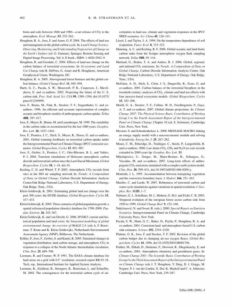
602 K. M. STRASSMANN ET AL.
biota and soils between 1860 and 1980—a net release of CO2 to theatmosphere. Ecol. Monogr. 53, 235–262.
Houghton, R. A., Joos, F. and Asner, G. P. 2004. The effects of land useand managment on the global carbon cycle. In: Land Change Science:Observing, Monitoring, and Understanding Trajectories of Change onthe Earth’s Surface (ed. G. Gutman), Springer, Remote Sensing andDigital Image Processing, Vol. 6, E-book., ISBN: 1-4020-2562–9.
Houghton, R. and Goodale, C. 2004. Effects of land-use change on thecarbon balance of terrestrial ecosystems. In: Ecosystems and LandUse Change (eds R. DeFries, G. Asner and R. Houghton), AmericanGeophysical Union, Washington, DC.
Houghton, R. A. 2005. Aboveground forest biomass and the global car-bon balance. Global Change Biol. 11, 945–958.
Hurtt, G. C., Pacala, S. W., Moorcroft, P. R., Caspersen, J., Shevli-akova, E. and co-authors. 2002. Projecting the future of the U. S.carbon sink. Proc. Natl. Acad. Sci. USA 99, 1389–1394, doi:10.1073/pnas.012249999.
Joos, F., Bruno, M., Fink, R., Stocker, T. F., Siegenthaler, U. and co-authors. 1996. An efficient and accurate representation of complexoceanic and biospheric models of anthropogenic carbon uptake. Tellus48B, 397–417.
Joos, F., Meyer, R., Bruno, M. and Leuenberger, M. 1999. The variabilityin the carbon sinks as reconstructed for the last 1000 years. Geophys.Res. Lett. 26, 1437–1441.
Joos, F., Prentice, I. C., Sitch, S., Meyer, R., Hooss, G. and co-authors.2001. Global warming feedbacks on terrestrial carbon uptake underthe Intergovernmental Panel on Climate Change (IPCC) emission sce-narios. Global Biogeochem. Cycles 15, 891–907.
Joos, F., Gerber, S., Prentice, I. C., Otto-Bliesner, B. L. and Valdes,P. J. 2004. Transient simulations of Holocene atmospheric carbondioxide and terrestrial carbon since the Last Glacial Maximum. GlobalBiogeochem. Cycles 18, 1–18. doi:10.
Keeling, C. D. and Whorf, T. P. 2003. Atmospheric CO2 records fromsites in the SIO air sampling network In: Trends: A Compendiumof Data on Global Change, Carbon Dioxide Information AnalysisCenter,Oak Ridge National Laboratory, U.S. Department of Energy,Oak Ridge, Tenn., USA.
Klein Goldewijk, K. 2001. Estimating global land use change over thepast 300 years: the HYDE database. Global Biogeochem. Cycles 15,417–433.
Klein Goldewijk, K. 2005. Three centuries of global population growth: aspatial referenced population (density) database for 1700–2000. Pop-ulat. Environ. 26, 343–367.
Klein Goldewijk, K. and van Drecht, G. 2006. HYDE3: current and his-torical population and land cover. In: Integrated modelling of globalenvironmental change. An overview of IMAGE 2.4. (eds A. F. Bouw-man, T. Kram and K. Klein Goldewijk), Netherlands EnvironmentalAssessment Agency (MNP), Bilthoven, The Netherlands.
Kohler, P., Joos, F., Gerber, S. and Knutti, R. 2005. Simulated changes invegetation distribution, land carbon storage, and atmospheric CO2 inresponse to a collapse of the North Atlantic thermohaline circulation.Clim. Dyn. 25, 689–708.
Leemans, R. and Cramer, W. P. 1991. The IIASA climate database forland areas on a grid with 0.5◦ resolution. research report RR-91-18.Tech. rep., International Institute for Applied System Analysis.
Leemans, R., Eickhout, B., Strengers, B., Bouwman, L. and Schaeffer,M. 2002. The consequences for the terrestrial carbon cycle of un-
certainties in land use, climate and vegetation responses in the IPCCSRES scenarios. Sci. China 45, 126–141.
Lloyd, J. and Taylor, J. A. 1994. On the temperature dependence of soilrespiration. Funct. Ecol. 8, 315–323.
Manning, A. C. and Keeling, R. F. 2006. Global oceanic and land bioticcarbon sinks from the Scripps atmospheric oxygen flask samplingnetwork. Tellus 58B, 95–116.
Marland, G., Boden, T. A. and Andres, R. J. 2006. Global, regional,and national CO2 emissions. In: Trends: A Compendium of Data onGlobal Change, Carbon Dioxide Information Analysis Center, OakRidge National Laboratory, U.S. Department of Energy, Oak Ridge,Tenn., USA.
McGuire, A. D., Sitch, S., Clein, J. S., Dargaville, R., Esser, G. andco-authors. 2001. Carbon balance of the terrestrial biosphere in thetwentieth century: analyses of CO2, climate and land use effects withfour process-based ecosystem models. Global Biogeochem. Cycles15, 183–206.
Meehl, G. A., Stocker, T. F., Collins, W. D., Friedlingstein, P., Gaye,A. T. and co-authors. 2007. Global climate projections. In: ClimateChange 2007: The Physical Science Basis. Contribution of WorkingGroup I to the Fourth Assessment Report of the IntergovernmentalPanel on Climate Change, Chapter 10 (ed. S. Solomon), CambridgeUniv. Press, New York.
Messner, S. and Schrattenholzer, L. 2000. MESSAGE-MACRO: linkingan energy supply model with a macroeconomic module and solvingit iteratively. Energy Int. J. 25, 267–282.
Meure, C. M., Etheridge, D., Trudinger, C., Steele, P., Langenfelds, R.and co-authors. 2006. Law dome CO2, CH4 and N2O ice core recordsextended to 2000 years bp. Geophys. Res. Lett. 33.
Mikolajewicz, U., Groger, M., Maier-Reimer, R., Schurgers, G.,Vizcaıno, M. and co-authors. 2007. Long-term effects of anthro-pogenic CO2 emissions simulated with a complex earth system model.Clim. Dyn. 28, 599–631, doi:10.1007/s00382-006-0204-y.
Monteith, J. L. 1995. Accommodation between transpiring vegetationand the convective boundary-layer. J. Hydrol. 166, 251–263.
Mueller, C. and Lucht, W. 2007. Robustness of terrestrial carbon andwater cycle simulations against variations in spatial resolution. J. Geo-phys. Res. 112D, 1–7.
Nabuurs, G. J., Schelhaas, M. J., Mohren, G. M.J. and Field, C. B. 2003.Temporal evolution of the european forest sector carbon sink from1950 to 1999. Global Change Biol. 9, 152–160.
Nakicenovic, N. and Swart, R. (eds.), 2000. Special Report on EmissionScenarios. Intergovernmental Panel on Climate Change, CambridgeUniversity Press, New York.
Pacala, S. W., Hurtt, G. C., Baker, D., Peylin, P., Houghton, R. A. andco-authors. 2001. Consistent land- and atmosphere-based U.S. carbonsink estimates. Science 292, 2316–2320.
Plattner, G. K., Joos, F. and Stocker, T. F. 2002. Revision of the globalcarbon budget due to changing air-sea oxygen fluxes. Global Bio-geochem. Cycles 16, 1096, doi:10.1029/2001GB001746.
Prather, M., Ehhalt, D., Dentener, F., Derwent, R., Dlugokencky, E. andco-authors. 2001. Atmospheric chemistry and greenhouse gases. In:Climate Change 2001: The Scientific Basis. Contribution of WorkingGroup I to the Third Assessment Report of the Intergovernmental Panelon Climate Change (eds J. T. Houghton, Y. Ding, D. J. Griggs, M.Noguer, P. J. van der Linden, X. Dai, K. Maskell and C. A. Johnson),Cambridge Univ. Press, New York, 239–287.
Tellus 60B (2008), 4
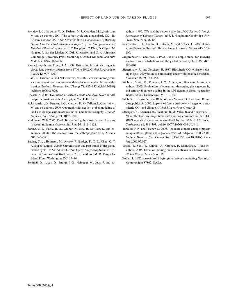
EFFECT OF LAND USE ON CARBON FLUXES 603
Prentice, I. C., Farquhar, G. D., Fasham, M. J., Goulden, M. I., Heimann,M. and co-authors. 2001. The carbon cycle and atmospheric CO2. In:Climate Change 2001: The Scientific Basis. Contribution of WorkingGroup I to the Third Assessment Report of the IntergovernmentalPanel on Climate Change (eds J. T. Houghton, Y. Ding, D. Griggs, M.Noguer, P. van der Linden, X. Dai, K. Maskell and C. A. Johnson),Cambridge University Press, Cambridge, United Kingdom and NewYork, NY, USA, 183–237.
Ramankutty, N. and Foley, J. A. 1999. Estimating historical changes inglobal land cover: croplands from 1700 to 1992. Global Biogeochem.Cycles 13, 997–1027.
Riahi, K., Grubler, A. and Nakicenovic, N. 2007. Scenarios of long-termsocio-economic and environmental development under climate stabi-lization. Technol. Forecast. Soc. Change 74, 887–935, doi:10.1016/j.techfore.2006.05.026.
Roesch, A. 2006. Evaluation of surface albedo and snow cover in AR4coupled climate models. J. Geophys. Res. 111D, 1–18.
Rokityanskiy, D., Benitez, P. C., Kraxner, F., McCallum, I., Obersteiner,M. and co-authors. 2006. Geographically explicit global modeling ofland-use change, carbon sequestration, and biomass supply. Technol.Forecast. Soc. Change 74, 1057–1082.
Ruddiman, W. F. 2005. Cold climate during the closest stage 11 analogto recent millennia. Quarter. Sci. Rev. 24, 1111–1121.
Sabine, C. L., Feely, R. A., Gruber, N., Key, R. M., Lee, K. and co-authors. 2004a. The oceanic sink for anthropogenic CO2. Science305, 367–371.
Sabine, C. L., Heimann, M., Artaxo, P., Bakker, D. C. E., Chen, C. T.A. and co-authors. 2004b. Current status and past trends of the globalcarbon cycle. In: The Global Carbon Cycle: Integrating Humans, Cli-mate and the Natural World (eds C. B. Field and M. R. Raupach),Island Press, Washington, DC, 17–44.
Schimel, D., Alves, D., Enting, I. G., Heimann, M., Joos, F. and co-
authors. 1996. CO2 and the carbon cycle. In: IPCC Second ScientificAssessment of Climate Change (ed. J. T. Houghton), Cambridge Univ.Press, New York, 76–86.
Seneviratne, S. I., Lanthi, D., Litschi, M. and Schaer, C. 2006. Land-atmosphere coupling and climate change in europe. Nature 443, 205–209.
Siegenthaler, U. and Joos, F. 1992. Use of a simple model for studyingoceanic tracer distributions and the global carbon cycle. Tellus 44B,186–207.
Siegenthaler, U. and Oeschger, H. 1987. Biospheric CO2 emissions dur-ing the past 200 years reconstructed by deconvolution of ice core data.Tellus Ser. B, 39, 140–154.
Sitch, S., Smith, B., Prentice, I. C., Arneth, A., Bondeau, A. and co-authors. 2003. Evaluation of ecosystem dynamics, plant geographyand terrestrial carbon cycling in the LPJ dynamic global vegetationmodel. Global Change Biol. 9, 161–185.
Sitch, S., Brovkin, V., von Bloh, W., van Vuuren, D., Eickhout, B. andGanopolski, A. 2005. Impacts of future land cover changes on atmo-spheric CO2 and climate. Global Biogeochem. Cycles 19.
Strengers, B., Leemans, R., Eickhout, B., de Vries, B. and Bouwman, L.2004. The land-use projections and resulting emissions in the IPCCSRES scenarios scenarios as simulated by the IMAGE 2.2 model.GeoJournal 61, 381–393, doi:10.1007/s10708-004-5054-8.
Tubiello, F. N. and Fischer, G. 2006. Reducing climate change impactson agriculture: global and regional effects of mitigation, 2000-2080.Technol. Forecast. Soc. Change 74, 1030–1056, doi:10.1016/j. tech-fore.2006.05.027.
Vesala, T., Suni, T., Rannik, U., Keronen, P., Markkanen, T. and co-authors. 2005. Effect of thinning on surface fluxes in a boreal forest.Global Biogeochem. Cycles 19.
Zobler, L. 1986. A world soil file for global climate modelling. TechnicalMemorandum 87802, NASA.
Tellus 60B (2008), 4