Simulating Combustion in Spark-Ignition Engines with … · Simulating Combustion in Spark-Ignition...

Simulating Combustion in Spark-Ignition Engines with ANSYS CFX

Dirk Linse, Bodo Durst and Christian Hasse Powertrain - CAE Combustion BMW Group, Munich Stefano Toninel, Thomas Frank and Hendrik Forkel ANSYS Germany SYNOPSIS In order to investigate Gasoline Direct Injection engines (GDI) by means of 3D-CFD simulations an efficient and innovative workflow for automated mesh generation is used which is based on the Pistongrid infrastructure provided by ANSYS CFX. This workflow was developed by BMW and has been established in the powertrain design process. For the simulation of combustion in Spark Ignition engines (SI) the G-equation model for fully and partially premixed combustion was successfully implemented in the ANSYS CFX code and coupled with the framework for simulating spark-ignition and predicting species in the reacted mixture by means of flamelet libraries. The level-set based combustion model is presented and discussed in detail. Based on experimental results, 3D simulations for a turbo-charged gasoline direct injection engine are carried out, taking into account residual gas, spray, spray-wall interaction and combustion. The results are compared to experimental data. 1. INTRODUCTION The new BMW generation of turbo-charged gasoline engine (TVDI) represents a major step in the evolution of gasoline engines. The combination of various technology generations such as TwinPower Turbo, High Precision Injection and VALVETRONIC, allows to significantly improve fuel efficiency and emission levels while at the same time the performance of the engine is maintained or even improved. In order to optimize engine performance and to obtain a more complete understanding of the underlying physical processes, experimental and numerical tools are used in a combined fashion. Especially the 3D-CFD simulation of in-cylinder flow is a powerful tool which enables a better understanding of physical phenomena like mixture formation and combustion. In order to make the ANSYS CFX code suitable for the increasing complexity of BMW turbo-charged GDI engines, which are characterized by complex geometry, fully variable valvetrain (VALVETRONIC), cam-phasing (VANOS) etc., an efficient and innovative workflow for fully automated mesh generation was developed. However, the three-dimensional simulation of turbulent reacting flows in Internal Combustion Engines (ICE) still represents one of the most challenging applications of Computational Fluid Dynamics (CFD). A promising model for combustion simulation in SI engines is the G-equation, which was successfully implemented in ANSYS CFX. The model is based on a level-set approach which provides a geometrical description of the flame front and other attractive features which are emphasized and discussed in the following sections. In the first part, the different development and analysis tools, engine test bench, 1D gas exchange simulation coupled with heat release analysis and 3D-CFD simulation, respectively

EASC 20094th European Automotive Simulation Conference

Munich, Germany6-7 July 2009

1

are presented. In the next section, the combustion regime for turbo-charged GDI engines is analyzed using the Peters-Borghi diagram followed by an introduction of the G-equation and the spark-ignition model. A brief overview of the workflow for the automated mesh generation is given and the numerical setup for the 3D-CFD calculation is summarized. In the last section, results for a turbo-charged GDI engine are presented and compared to experimental data. 2. DEVELOPMENT TOOLS The development of advanced combustion engines, to cope with increasing demands with respect to emissions and fuel consumption, is nowadays only possible with a combination of experimental and simulation methods. In the engine development process at BMW, schematically shown in Figure 1, following development tools are used together in order to analyze and optimize the combustion process:

• Engine test bench with low- and high-pressure indication

• 1D gas exchange simulation and heat release analysis

• 3D-CFD simulation The first step is to obtain the experimental data on the engine test bench. The pressure in the intake and exhaust manifold is measured using low-pressure indication while the pressure in the combustion chamber is measured using high-pressure indication. Additionally, corresponding temperature measurements are taken in the intake and exhaust system.

Figure 1: Development tools The next step is the evaluation of the heat release and its integral value based on the measured pressure in the combustion chamber. The heat release analysis is appropriate if only a global assessment of the combustion process is needed. The gas exchange process and the resulting mass flow are calculated from the measured pressure traces, using 1D gas exchange simulation software. With regards to 3D-CFD simulation, it is crucial to reproduce the gas exchange process to determine the correct boundary conditions at the intake and exhaust port and the corresponding initial conditions. Finally, 3D simulations are carried out to obtain detailed information on different processes such as spray, mixture formation, flow structure and combustion. Advances in high performance computing and Computational



2

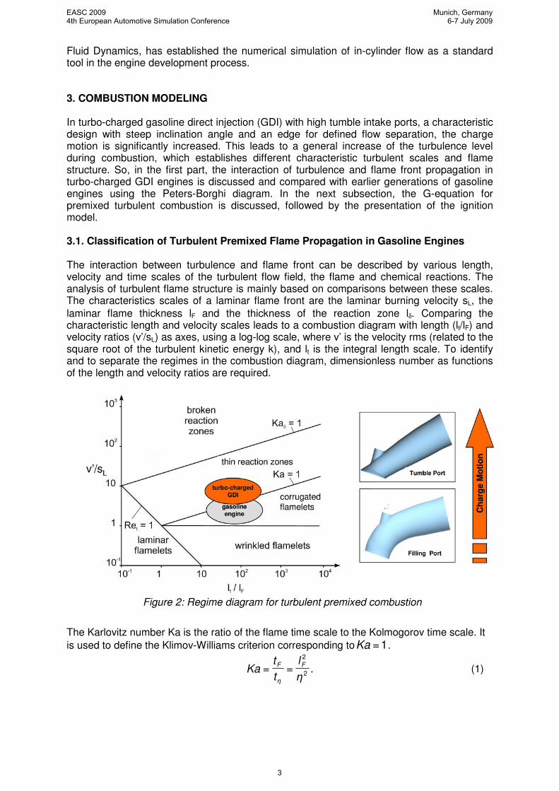
Fluid Dynamics, has established the numerical simulation of in-cylinder flow as a standard tool in the engine development process. 3. COMBUSTION MODELING In turbo-charged gasoline direct injection (GDI) with high tumble intake ports, a characteristic design with steep inclination angle and an edge for defined flow separation, the charge motion is significantly increased. This leads to a general increase of the turbulence level during combustion, which establishes different characteristic turbulent scales and flame structure. So, in the first part, the interaction of turbulence and flame front propagation in turbo-charged GDI engines is discussed and compared with earlier generations of gasoline engines using the Peters-Borghi diagram. In the next subsection, the G-equation for premixed turbulent combustion is discussed, followed by the presentation of the ignition model. 3.1. Classification of Turbulent Premixed Flame Propagation in Gasoline Engines The interaction between turbulence and flame front can be described by various length, velocity and time scales of the turbulent flow field, the flame and chemical reactions. The analysis of turbulent flame structure is mainly based on comparisons between these scales. The characteristics scales of a laminar flame front are the laminar burning velocity sL, the

laminar flame thickness lF and the thickness of the reaction zone lδ. Comparing the characteristic length and velocity scales leads to a combustion diagram with length (lt/lF) and velocity ratios (v’/sL) as axes, using a log-log scale, where v’ is the velocity rms (related to the square root of the turbulent kinetic energy k), and lt is the integral length scale. To identify and to separate the regimes in the combustion diagram, dimensionless number as functions of the length and velocity ratios are required.

Figure 2: Regime diagram for turbulent premixed combustion

The Karlovitz number Ka is the ratio of the flame time scale to the Kolmogorov time scale. It

is used to define the Klimov-Williams criterion corresponding to 1=Ka .

.== 2

2

η

l

t

tKa

F

η

F

(1)



3

For Karlovitz numbers greater than unity, the smallest eddies are able to penetrate into the preheat zone, but not necessarily into the reaction zones. Since the thickness of the reaction zone is much thinner than the laminar flame thickness, one may introduce a Karlovitz

number Kaδ which compares the thickness of the reaction zone to the Kolmogorov scale. In Figure 2 the combustion regime according to Peters [1] is presented. For engine combustion, the two most important regimes are the corrugated flamelet and thin reactions regime. It was shown in Wirth [2] that for earlier generations of gasoline engines, the combustion mainly takes place in the corrugated flamelet regime, where the turbulent eddies wrinkle the flame, leading to an increase of the flame front surface. However, they are not able to penetrate into the preheat zone and the inner structure remains laminar. Newer generations of gasoline engines especially with turbo charging and direct injection, require a significantly increased charge motion and higher turbulence level. Based on a numerical and experimental analysis of the flame structure in a turbo-charged GDI engine, Linse [3] has shown that the expected combustion process takes place in the thin reaction zones regime. Here, the smallest eddies close to the Kolmogorov size can enter and thicken the preheat zone. Although this analysis leads only to a qualitative classification of combustion regime based on characteristic numbers, it supports to derive and to choose appropriate turbulent combustion models corresponding to a specific regime. These results show that for the prediction of the combustion process in turbo-charged gasoline engines, the turbulent combustion model has to be valid in the corrugated flamelet regime as well as in the regime of thin reaction zones. 3.2. Modelling premixed turbulent combustion based on the G-Equation Most of the turbulent combustion models assume scale separation so that the locally instantaneous flame front can be modelled as a laminar premixed flame, stretched and deformed by turbulent structures. The assumption of scale separation is also referred to as the flamelet concept, which means that chemistry and turbulence can be regarded as decoupled. In this particular case, the chemistry can be calculated a priori for a small set of thermodynamical parameters such as pressure, mixture fraction and temperature: the corresponding species compositions are then stored in flamelet libraries. So, the main challenge in modelling turbulent premixed combustion is then the prediction of the flame front propagation or the estimation of the probability of finding burnt and unburnt gases. In the Burning Velocity Model (BVM) and the Extended Coherent Flame Model (ECFM), see ANSYS CFX [4], the numerical tracking of a turbulent premixed flame is accomplished by solving a transport equation for the so-called reaction progress variable, c. This quantity varies in the range between 0 (fresh mixture) and 1 (burnt gases) and may be viewed as the probability of finding combustion products. The main difference between the two models is the closure of the chemical source term. In the BVM an algebraic correlation is used, based on the turbulent burning velocity sT. The ECFM, instead, describes the mean reaction rate in terms of the flame surface area, a combination of the laminar burning velocity sL and the

flame surface density Σ. The latter quantity is computed by solving an additional transport equation. These models are derived based on the assumption that the flame front is infinitely thin. As already shown in the previous section, the combustion process in turbo-charged direct injection gasoline engines is expected to take place in the regime of thin reaction zones, where the smallest eddies are able to penetrate into the preheat zone and to thicken the flame. In contrast to the BVM and ECFM the G-Equation Model is rigorously modelled for the corrugated flame and thin reaction regime and, a priori, does not require that the instantaneous flame is a discontinuity in the flow field. This makes the G-equation very attractive as a combustion model for the simulation of modern turbo-charged GDI engines.

In the G-equation model, the tracking of the turbulent flame is based on the level-set approach, where the flame front is identified as the surface G0, separating burnt and unburnt gases, thus leading to the following position of the flame front:



4

flame=),( 0 ⇔GtG x (2)

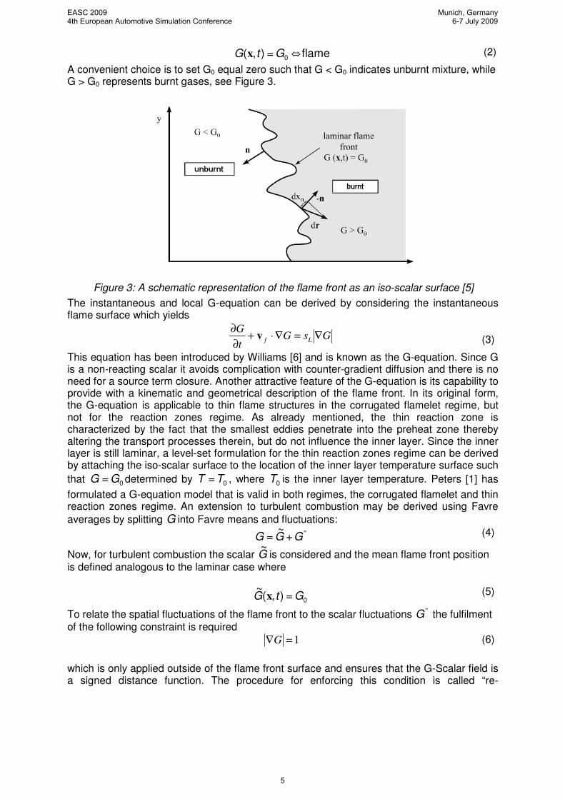
A convenient choice is to set G0 equal zero such that G < G0 indicates unburnt mixture, while G > G0 represents burnt gases, see Figure 3.

Figure 3: A schematic representation of the flame front as an iso-scalar surface [5]

The instantaneous and local G-equation can be derived by considering the instantaneous flame surface which yields

GsGt

GLf ∇=∇⋅+

∂

∂v

(3)

This equation has been introduced by Williams [6] and is known as the G-equation. Since G is a non-reacting scalar it avoids complication with counter-gradient diffusion and there is no need for a source term closure. Another attractive feature of the G-equation is its capability to provide with a kinematic and geometrical description of the flame front. In its original form, the G-equation is applicable to thin flame structures in the corrugated flamelet regime, but not for the reaction zones regime. As already mentioned, the thin reaction zone is characterized by the fact that the smallest eddies penetrate into the preheat zone thereby altering the transport processes therein, but do not influence the inner layer. Since the inner layer is still laminar, a level-set formulation for the thin reaction zones regime can be derived by attaching the iso-scalar surface to the location of the inner layer temperature surface such

that 0= GG determined by 0=TT , where 0T is the inner layer temperature. Peters [1] has

formulated a G-equation model that is valid in both regimes, the corrugated flamelet and thin reaction zones regime. An extension to turbulent combustion may be derived using Favre

averages by splitting G into Favre means and fluctuations:

''+~

= GGG (4)

Now, for turbulent combustion the scalar G~

is considered and the mean flame front position is defined analogous to the laminar case where

0=),(~

GtG x

(5)

To relate the spatial fluctuations of the flame front to the scalar fluctuations ''G the fulfilment of the following constraint is required ∇G = 1

(6)

which is only applied outside of the flame front surface and ensures that the G-Scalar field is a signed distance function. The procedure for enforcing this condition is called “re-



5

initialization” and is probably the most critical part of the level-set approach. In this work, an innovative method is used which is explained in detail in [7]. The modelling of the G-equation is extensively explained by Peters [1] and is summarized by the following transport equations for the mean value of the G-Scalar and its variance:

ρ ∂ ˜ G

∂ t+ ρ ˜ v ⋅ ∇ ˜ G = ρ sT

0( ) ∇ ˜ G − ρ ′ D t ˜ κ ∇ ˜ G

(7)

( ) ( ) 222

||||

22 ~

~

~~2

~~~

~

Gk

cGDGDGt

Gstt

′′−∇+′′∇⋅∇=′′∇⋅+∂

′′∂ ερρρρρ v

(8)

The || subscript in the G-variance diffusion term indicates that only the turbulent diffusion tangential to the mean flame front is accounted for. The flame curvature κ is defined in terms of the G-field

κ = ∇ ⋅ n n = −∇ ˜ G

∇ ˜ G

(9)

It is positive if the flame is convex with respect to the unburnt mixture. The turbulent diffusivity of the curvature term in Equation 6 is expressed in analogy to a mixing length approach by using the turbulent flame brush thickness as length scale, resulting in

′ D t =cµcs

2Sc t

l f ,tk1/ 2

(10)

The turbulent brush thickness lF,t is defined as the square root of the G-variance normalized by the gradient of the G-scalar and represents the link between the two transported quantities of the G-equation model. Since the G-variance is a measure for the fluctuations of the instantaneous flame fronts about their mean position, the standard deviation is a plausible measure for the turbulent flame brush thickness:

G

Gl tf ~

~ 2

,

∇

′′=

(11)

The turbulent burning velocity 0Ts of a planar flame is modelled by means of an algebraic

correlation ( )

tLT σss +1=

(12)

The turbulent flame surface area ratio σt denotes the increase of flame surface due to

turbulence effects. Using the relationship according to Ewald [8] yields

++

−=

ks

lbcl

Sc

cc

b

bl

Sc

cc

b

b

l

l

L

fsq

t

sq

t

s

f

tf

t

εσ

µµ

2

3

16

3

4

2

32*

2

1

4

3*

1

2

3,

(13)

Ewald’s closure for the turbulent burning velocity consists essentially of the same correlation proposed by Peters corrected by the factor l*. This factor accounts for instationary effects of a developing turbulent flame front measured by the relationship between the turbulent flame thickness and the algebraic flame brush thickness and is given by

lg,,

,*

atf

tf

l

ll =

(14)



6

The condition l* = 0 denotes a laminar flame while l* = 1 represents a fully developed flame front. For a fully developed turbulent flame in steady state, the algebraic flame brush thickness is proportional to the turbulent length scale and can be computed according to Equation 8 by using an equilibrium solution of the G-variance:

l f ,t,a lg =

˜ ′ ′ G a lg

2

∇ ˜ G =

2cµ

csSct

k3 / 2

ε

(15)

The coefficients for the turbulent burning velocity closure are summarized in Table 1. The coupling of the G-equation in ANSYS CFX with the flamelet libraries is accomplished by computing the reaction progress variable. Unlike the BVM and ECFM, where a transport equation is solved for that quantity, the reaction progress is derived from the G-scalar and G-variance, by assuming that the PDF of G is Gaussian distribution: ( )

∫∞

=

′′

−−

′′=

02

2

2~

2

~

exp~2

1

GGdG

G

GG

Gc

π

(16)

A more detailed description of the implementation in ANSYS CFX and model validation regarding mesh sensitivity and robustness is given in [7].

Coefficient Value

b1 2.0

b3 1.0

cs 2.0

q 0.66

cµ 0.09

ct 0.70

Table 1: Coefficients for turbulent burning

velocity closure according to Ewald [8] 3.3 Spark Ignition Model The spark-kernel model available in ANSYS CFX [4] solves an ordinary differential equation describing the growth rate of the kernel radius as a function of the turbulent burning velocity:

kT

b

uk sdt

dr,

ρ

ρ=

(17)

The density ratio ρu/ρb and sT,k are evaluated by averaging the corresponding quantities computed by ANSYS CFX over a spherical domain, centred on the initial spark-location and with a constant, user-defined radius, rT. This region acts like a mask interfacing the 0D model to the 3D flow-solver. The turbulent burning velocity sT,k is modelled according to the closure correlation suggested by Ewald and with a modification accounting for high curvature when the kernel is small:

εµ

2

, ,2

,maxk

Sc

cDD

rsss

t

tt

k

TLkT =

−=

(18)

Generally speaking, the purpose of an ignition model is to initialize and update the primary combustion variables during the early stages of the flame propagation, when the kernel-size



7

is below the grid resolution and therefore cannot be solved by the 3D code. Then the quantities are mapped back from the spark-model to the flow-solver. The 0D model is switched off and the control is transferred back to the transport equation for the flame propagation when the kernel radius rk reaches the prescribed value rT. In order to ensure a smooth transition, rT should be sufficiently large so that the mask region can be resolved by the mesh. In the G-equation model, during the kernel growth (rk < rT) the G-scalar is computed by simply enforcing a spherical distribution with G0 located at a distance rk from the ignition point: 222

)(),,,( zyxtrtzyxG k ++−=

(19)

This is a remarkable feature of the level-set approach, since a new flame front, even in multiple instances like in multi-spark ignition can be easily initialized, just by feeding a function describing analytically the geometrical shape of the interface. 4. EXPERIMENTAL AND NUMERICAL SETUP 4.1. Experiment The experimental investigations were performed on a BMW turbo-charged gasoline engine with variable valve timing and lift. Detailed engine specific data are confidential and will not be published. Measurements and simulations are performed for a high load engine operating point at 6500 rpm. 4.2. Automated Mesh Generation Substantial improvements have been achieved in numerics and the mathematical description of physical processes such that CFD simulation is now established as a design tool in the engine development process. However, an obstacle to the use of CFD in the development process is still the mesh generation. In the past, the mesh generation was difficult and time consuming because the manual mesh generation techniques required considerable expertise and effort to account for the complex shapes and moving parts of the combustion chamber as well as intake and exhaust system. Another import aspect is that the topology and quality of the generated mesh can differ from user to user and the comparability of CFD results is not guaranteed. This promotes the need for a robust and efficient dynamic mesh generation method to ensure the overall mesh quality and to reduce the user interaction time. In the following, a short overview of the automated meshing process used at BMW is given, which is characterized by its great flexibility with respect to mesh structure and geometry-handling, including the options to:

• decompose the engine geometry into moving and stationary parts to reduce interpolation errors and to enhance the robustness of the re-meshing process

• work with hybrid meshes, comprised of tetrahedra, prisms and hexahedra

• locally identify and to replace degenerated tetrahedral (local remeshing) instead of remeshing the complete computational domain

• work with extrusion meshes to use structured quad/hexahedral elements

• implement a hexahedral mesh for the narrow valve gaps between valve seat rings and intake valves



8

• introduce local mesh densities in critical regions for, e.g. intake valve masking or spray cone densities for a better representation of the penetration depth

The dynamic mesh preparation is controlled by ANSYS CFX Pistongrid which stops the run when the mesh quality falls below a certain threshold and calls the user defined meshing scripts to generate a new mesh with the correct position of the intake/exhaust valves and piston. A detailed description of the automated meshing process and the main differences to the standard Pistongrid workflow is given in [9]. 4.3. General Settings In order to reduce numerical diffusion we apply the high resolution scheme for spatial discretization and second order backward Euler scheme throughout the computation. The

physical time step during combustion and injection is 6-128.5 et =∆ s which corresponds to

2.0=∆CA for 6500 RPM. For the in-cylinder simulations a customized executable of the current CFX-12 release is used. 4.4. Turbulence Modelling ANSYS CFX provides several turbulence models and associated wall functions for the calculation of the turbulent Reynolds stresses, scalar fluxes and the characteristic time and length scales. In the RANS context, the most widely used turbulence model is still the well known k -εmodel. Over the years, it has proven to be stable and numerically robust

providing good predictions for many flows of engineering interest. Some more recent variants like the k -ω based Shear-Stress-Transport (SST) model may be more appropriate to

represent flows with boundary layer separation, sudden changes in mean strain rate and flows in rotating fluids [4]. Although the SST model has shown in some applications that it is superior to the k -ε model, it has not yet been properly assessed in the engine context.

Therefore, we use the standard k -ε turbulence model in combination with the Kato-Launder

limiter to suppress the excessive production of turbulence kinetic energy in stagnation regions. It should be noted that the turbulence parameters k and ε are particularly mesh

sensitive, tending to be underestimated on a coarse mesh. Fortunately the turbulence intensity v’ and the integral length scale lt, which determine important quantities like turbulent diffusion coefficients and turbulent burning velocities, are less mesh sensitive 4.5. Spray and Spray-Wall Interaction The modelling of fuel injection process is an essential part of an engine simulation. This has always been the case for Diesel engines and has come to be of increasing importance for SI engines with direct-injection. Models of different levels of capability are now available for nearly all fuel injection processes like nozzle flow, spray motion, evaporation, wall impingement and wall film formation. In general, however, it is still necessary to empirically tune coefficients or other inputs to the models by reference to experimental data to obtain satisfactory quantitative predictions. In this study, we initialize the particles after primary and secondary break-up. To match the experimental data we fitted the spray shape to available visualizations by specifying the initial droplet velocity, size and distribution. For the determination of these parameters for a wide range of operating points we are using data obtained by Design of Experiments (DoE) investigation, which is implemented via User Routines in CFX. Hence, the parameters are dynamically adjusted during the simulation, e.g. to account for increasing/decreasing pressure in the combustion chamber. Moreover, for a better representation of the penetration depth, local mesh densities in spray areas are introduced, especially near the injector tip where large velocity gradients occur. For the



9

simulation of spray-wall interaction we use a customized model, featuring particle break-up, wall film formation, droplet and film evaporation as well as non-ideal reflection. 4.6. Combustion Settings The combustion is calculated using the level-set based G-equation model presented in section 3. Pressure and temperature dependent flame libraries are used in order to recover the variation of CO2 dissociation depending on the local thermodynamic conditions. The laminar burning velocity and flame thickness are a priori calculated for a wide range of unburnt conditions, taken into account pressure and temperature dependencies as well as mixture fraction and residual gas variation, using one-dimensional flame computations. For the calculation of the turbulent burning velocity we are using Ewald’s correlation. 5. RESULTS

In this section, computational results for a turbo-charged GDI are presented. At first, the results for the gas exchange simulation including spray and mixture formation are presented followed by the results of the combustion simulation.

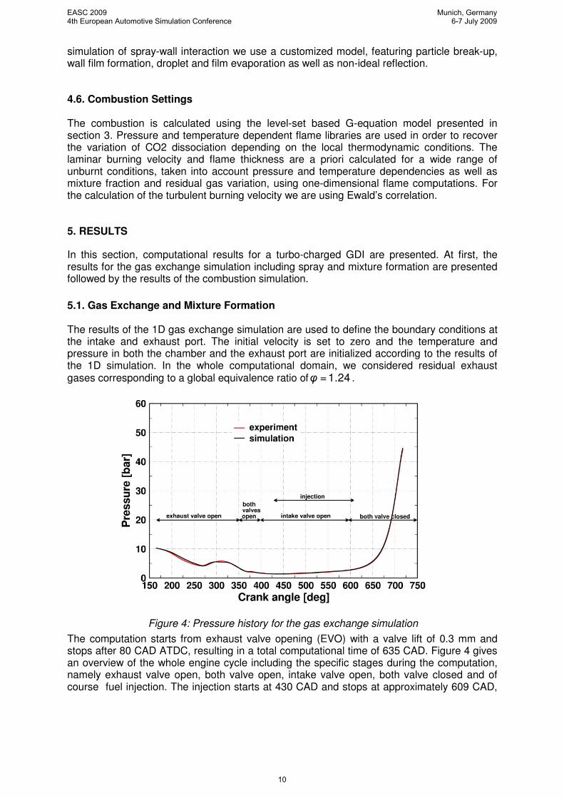
5.1. Gas Exchange and Mixture Formation The results of the 1D gas exchange simulation are used to define the boundary conditions at the intake and exhaust port. The initial velocity is set to zero and the temperature and pressure in both the chamber and the exhaust port are initialized according to the results of the 1D simulation. In the whole computational domain, we considered residual exhaust gases corresponding to a global equivalence ratio of 24.1=φ .

Figure 4: Pressure history for the gas exchange simulation

The computation starts from exhaust valve opening (EVO) with a valve lift of 0.3 mm and stops after 80 CAD ATDC, resulting in a total computational time of 635 CAD. Figure 4 gives an overview of the whole engine cycle including the specific stages during the computation, namely exhaust valve open, both valve open, intake valve open, both valve closed and of course fuel injection. The injection starts at 430 CAD and stops at approximately 609 CAD,



10

leading to a global equivalence ratio of 24.1=φ . The computed pressure history is in good

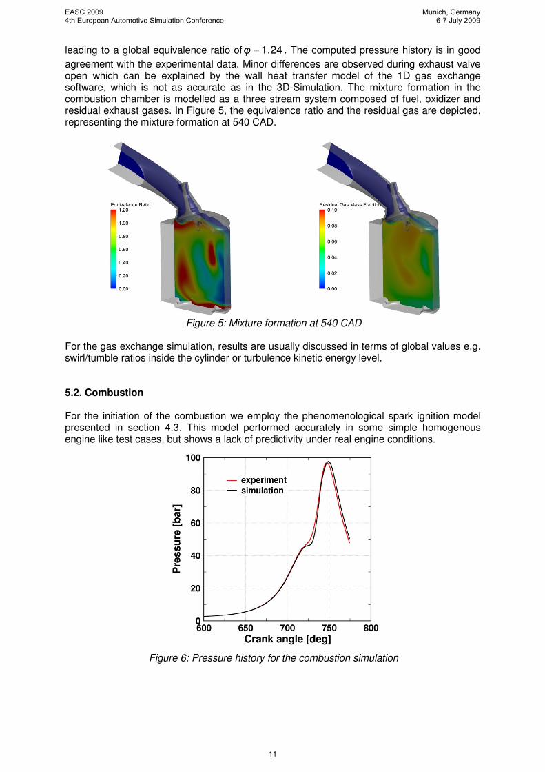
agreement with the experimental data. Minor differences are observed during exhaust valve open which can be explained by the wall heat transfer model of the 1D gas exchange software, which is not as accurate as in the 3D-Simulation. The mixture formation in the combustion chamber is modelled as a three stream system composed of fuel, oxidizer and residual exhaust gases. In Figure 5, the equivalence ratio and the residual gas are depicted, representing the mixture formation at 540 CAD.

Figure 5: Mixture formation at 540 CAD

For the gas exchange simulation, results are usually discussed in terms of global values e.g. swirl/tumble ratios inside the cylinder or turbulence kinetic energy level. 5.2. Combustion For the initiation of the combustion we employ the phenomenological spark ignition model presented in section 4.3. This model performed accurately in some simple homogenous engine like test cases, but shows a lack of predictivity under real engine conditions.

Figure 6: Pressure history for the combustion simulation



11

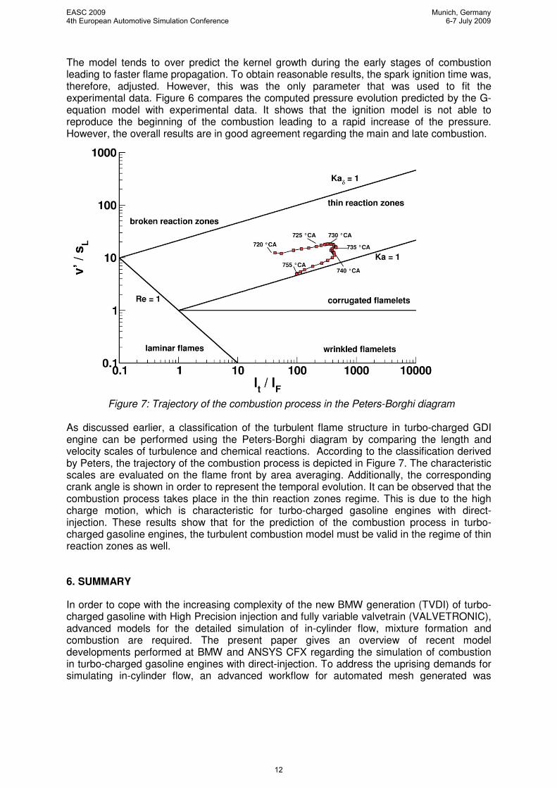
The model tends to over predict the kernel growth during the early stages of combustion leading to faster flame propagation. To obtain reasonable results, the spark ignition time was, therefore, adjusted. However, this was the only parameter that was used to fit the experimental data. Figure 6 compares the computed pressure evolution predicted by the G-equation model with experimental data. It shows that the ignition model is not able to reproduce the beginning of the combustion leading to a rapid increase of the pressure. However, the overall results are in good agreement regarding the main and late combustion.

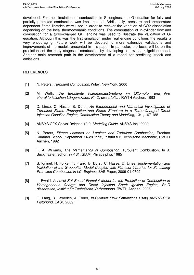
Figure 7: Trajectory of the combustion process in the Peters-Borghi diagram

As discussed earlier, a classification of the turbulent flame structure in turbo-charged GDI engine can be performed using the Peters-Borghi diagram by comparing the length and velocity scales of turbulence and chemical reactions. According to the classification derived by Peters, the trajectory of the combustion process is depicted in Figure 7. The characteristic scales are evaluated on the flame front by area averaging. Additionally, the corresponding crank angle is shown in order to represent the temporal evolution. It can be observed that the combustion process takes place in the thin reaction zones regime. This is due to the high charge motion, which is characteristic for turbo-charged gasoline engines with direct-injection. These results show that for the prediction of the combustion process in turbo-charged gasoline engines, the turbulent combustion model must be valid in the regime of thin reaction zones as well. 6. SUMMARY

In order to cope with the increasing complexity of the new BMW generation (TVDI) of turbo-charged gasoline with High Precision injection and fully variable valvetrain (VALVETRONIC), advanced models for the detailed simulation of in-cylinder flow, mixture formation and combustion are required. The present paper gives an overview of recent model developments performed at BMW and ANSYS CFX regarding the simulation of combustion in turbo-charged gasoline engines with direct-injection. To address the uprising demands for simulating in-cylinder flow, an advanced workflow for automated mesh generated was



12

developed. For the simulation of combustion in SI engines, the G-equation for fully and partially premixed combustion was implemented. Additionally, pressure and temperature dependent flame libraries were used in order to recover the variation of CO2 dissociation depending on the local thermodynamic conditions. The computation of in-cylinder flow and combustion for a turbo-charged GDI engine was used to illustrate the validation of G-equation. Although this was the first simulation under real engine conditions the results a very encouraging. Future work will be devoted to more extensive validations and improvements of the models presented in this paper. In particular, the focus will be on the predictions of the early stages of combustion by developing a new spark ignition model. Another main research path is the development of a model for predicting knock and emissions.

REFERENCES

[1] N. Peters, Turbulent Combustion, Wiley, New York, 2000

[2] M. Wirth, Die turbulente Flammenausbreitung im Ottomotor und ihre charakteristischen Längenskalen, Ph.D. dissertation, RWTH Aachen, 1993

[3] D. Linse, C. Hasse, B. Durst, An Experimental and Numerical Investigation of Turbulent Flame Propagation and Flame Structure in a Turbo-Charged Direct Injection Gasoline Engine, Combustion Theory and Modelling, 13:1, 167-188

[4] ANSYS CFX-Solver Release 12.0, Modeling Guide, ANSYS Inc., 2009

[5] N. Peters, Fifteen Lectures on Laminar and Turbulent Combustion, Ercoftac Summer School, September 14-28 1992, Institut für Technische Mechanik, RWTH Aachen, 1992

[6] F. A. Williams, The Mathematics of Combustion, Turbulent Combustion, In J. Buckmaster, editor, 97-131, SIAM, Philadelphia, 1985

[7] S.Toninel, H. Forkel, T. Frank, B. Durst, C. Hasse, D. Linse, Implementation and Validation of the G-equation Model Coupled with Flamelet Libraries for Simulating Premixed Combustion in I.C. Engines, SAE Paper, 2009-01-0709

[8] J. Ewald, A Level Set Based Flamelet Model for the Prediction of Combustion in Homogeneous Charge and Direct Injection Spark Ignition Engine, Ph.D dissertation, Institiut für Technische Verbrennung, RWTH Aachen, 2006

[9] G. Lang, B. Lewerich, J. Ebner, In-Cylinder Flow Simulations Using ANSYS-CFX Pistongrid, EASC,2009



13

Simulating Combustion in Spark-Ignition Engines with … · Simulating Combustion in Spark-Ignition...

Documents

Transcript of Simulating Combustion in Spark-Ignition Engines with … · Simulating Combustion in Spark-Ignition...