![Brownian Motion[1]](https://static.fdocuments.net/doc/165x107/577d35e21a28ab3a6b91ad47/brownian-motion1.jpg)
SIMULATING BROWNIAN MOTION...I) Simulating Brownian motion and Single Particle Trajectories This...
14
SIMULATING BROWNIAN MOTION ABSTRACT This exercise shows how to simulate the motion of single and multiple particles in one and two dimensions using Matlab. You will discover some useful ways to visualize and analyze particle motion data, as well as learn the Matlab code to accomplish these tasks. Once you understand the simulations, you can tweak the code to simulate the actual experimental conditions you choose for your study of Brownian motion of synthetic beads. These simulations will generate the predictions you can test in your experiment. In each section, Matlab code shown in the box to the left is used to generate the plot or analysis shown on the right. Please report in your lab book all values you obtain and answer to questions. To use the code, copy it from the box on the left, launch the Matlab application, and paste the code into the Matlab Command Window.
Transcript of SIMULATING BROWNIAN MOTION...I) Simulating Brownian motion and Single Particle Trajectories This...
SIMULATING BROWNIAN MOTION
ABSTRACT
This exercise shows how to simulate the motion of single and multiple particles in one and two dimensions using
Matlab. You will discover some useful ways to visualize and analyze particle motion data, as well as learn the
Matlab code to accomplish these tasks. Once you understand the simulations, you can tweak the code to simulate
the actual experimental conditions you choose for your study of Brownian motion of synthetic beads. These
simulations will generate the predictions you can test in your experiment. In each section, Matlab code shown in the
box to the left is used to generate the plot or analysis shown on the right. Please report in your lab book all values
you obtain and answer to questions. To use the code, copy it from the box on the left, launch the Matlab
application, and paste the code into the Matlab Command Window.
I) Simulating Brownian motion and Single Particle Trajectories
This exercise shows how to simulate the motion of a single particle in one and two dimensions. Brownian
motion in one dimension is composed of a sequence of normally distributed random displacements. The randn
function returns a matrix of a normally distributed random numbers with standard deviation 1. The two
arguments specify the size of the matrix, which will be 1xN in the example below. The first step in simulating
this process is to generate a vector of random displacements.
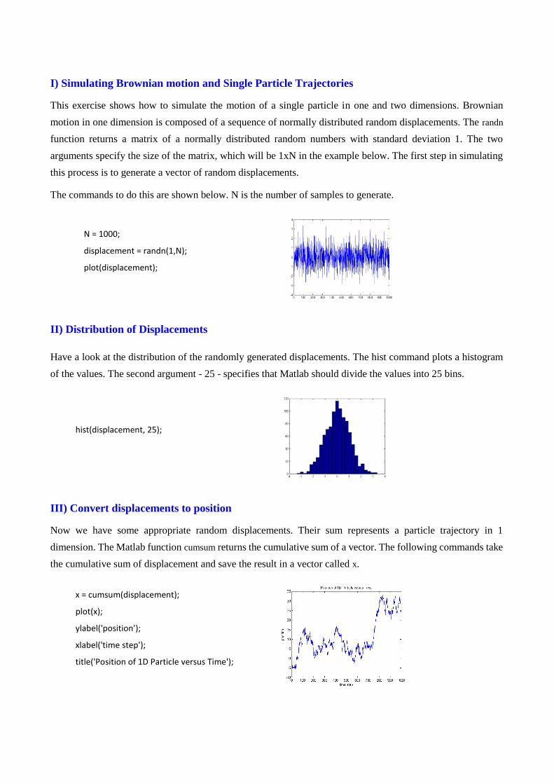
The commands to do this are shown below. N is the number of samples to generate.
N = 1000;
displacement = randn(1,N);
plot(displacement);
II) Distribution of Displacements
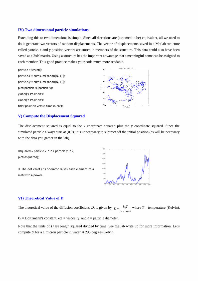
Have a look at the distribution of the randomly generated displacements. The hist command plots a histogram
of the values. The second argument - 25 - specifies that Matlab should divide the values into 25 bins.
hist(displacement, 25);
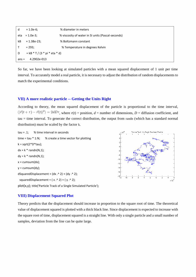
III) Convert displacements to position
Now we have some appropriate random displacements. Their sum represents a particle trajectory in 1
dimension. The Matlab function cumsum returns the cumulative sum of a vector. The following commands take
the cumulative sum of displacement and save the result in a vector called x.
x = cumsum(displacement);
plot(x);
ylabel('position');
xlabel('time step');
title('Position of 1D Particle versus Time');
IV) Two dimensional particle simulations
Extending this to two dimensions is simple. Since all directions are (assumed to be) equivalent, all we need to
do is generate two vectors of random displacements. The vector of displacements saved in a Matlab structure
called particle. x and y position vectors are stored in members of the structure. This data could also have been
saved as a 2xN matrix. Using a structure has the important advantage that a meaningful name can be assigned to
each member. This good practice makes your code much more readable.
particle = struct();
particle.x = cumsum( randn(N, 1) );
particle.y = cumsum( randn(N, 1) );
plot(particle.x, particle.y);
ylabel('Y Position');
xlabel('X Position');
title('position versus time in 2D');
V) Compute the Displacement Squared
The displacement squared is equal to the x coordinate squared plus the y coordinate squared. Since the
simulated particle always start at (0,0), it is unnecessary to subtract off the initial position (as will be necessary
with the data you gather in the lab).
dsquared = particle.x .^ 2 + particle.y .^ 2;
plot(dsquared);
% The dot caret (.^) operator raises each element of a
matrix to a power.
VI) Theoretical Value of D
The theoretical value of the diffusion coefficient, D, is given by 3
Bk TD
d
where T = temperature (Kelvin),
kB = Boltzmann's constant, eta = viscosity, and d = particle diameter.
Note that the units of D are length squared divided by time. See the lab write up for more information. Let's
compute D for a 1 micron particle in water at 293 degrees Kelvin.
d = 1.0e-6; % diameter in meters
eta = 1.0e-3; % viscosity of water in SI units (Pascal-seconds)
kB = 1.38e-23; % Boltzmann constant
T = 293; % Temperature in degrees Kelvin
D = kB * T / (3 * pi * eta * d)
ans = 4.2902e-013
So far, we have been looking at simulated particles with a mean squared displacement of 1 unit per time
interval. To accurately model a real particle, it is necessary to adjust the distribution of random displacements to
match the experimental conditions.
VII) A more realistic particle -- Getting the Units Right
According to theory, the mean squared displacement of the particle is proportional to the time interval,
, where r(t) = position, d = number of dimensions, D = diffusion coefficient, and
tau = time interval. To generate the correct distribution, the output from randn (which has a standard normal
distribution) must be scaled by the factor k.
tau = .1; % time interval in seconds
time = tau * 1:N; % create a time vector for plotting
k = sqrt(2*D*tau);
dx = k * randn(N,1);
dy = k * randn(N,1);
x = cumsum(dx);
y = cumsum(dy);
dSquaredDisplacement = (dx .^ 2) + (dy .^ 2);
squaredDisplacement = ( x .^ 2) + ( y .^ 2);
plot(x,y); title('Particle Track of a Single Simulated Particle');
VIII) Displacement Squared Plot
Theory predicts that the displacement should increase in proportion to the square root of time. The theoretical
value of displacement squared is plotted with a thick black line. Since displacement is expected to increase with
the square root of time, displacement squared is a straight line. With only a single particle and a small number of
samples, deviation from the line can be quite large.
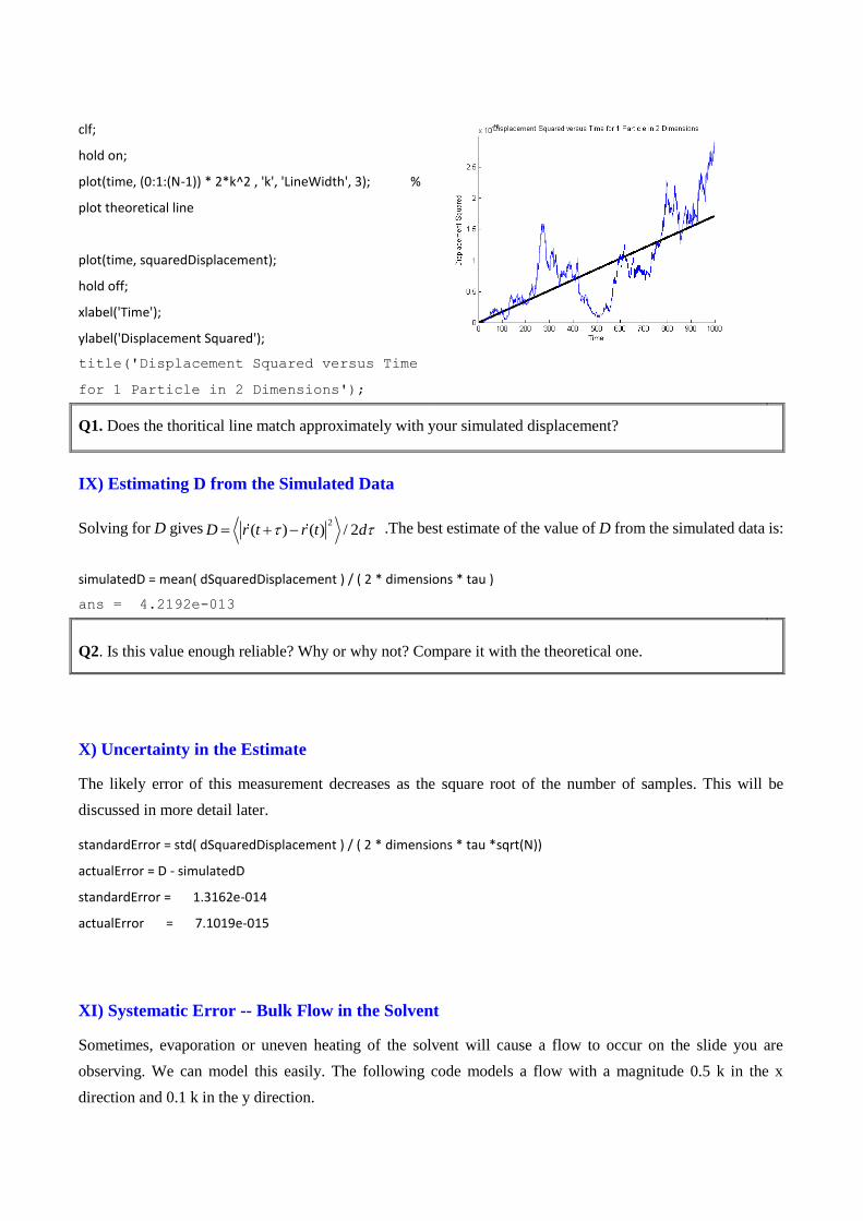
clf;
hold on;
plot(time, (0:1:(N-1)) * 2*k^2 , 'k', 'LineWidth', 3); %
plot theoretical line
plot(time, squaredDisplacement);
hold off;
xlabel('Time');
ylabel('Displacement Squared');
title('Displacement Squared versus Time
for 1 Particle in 2 Dimensions');
Q1. Does the thoritical line match approximately with your simulated displacement?
IX) Estimating D from the Simulated Data
Solving for D gives2
( ) ( ) / 2D r t r t d .The best estimate of the value of D from the simulated data is:
simulatedD = mean( dSquaredDisplacement ) / ( 2 * dimensions * tau )
ans = 4.2192e-013
Q2. Is this value enough reliable? Why or why not? Compare it with the theoretical one.
X) Uncertainty in the Estimate
The likely error of this measurement decreases as the square root of the number of samples. This will be
discussed in more detail later.
standardError = std( dSquaredDisplacement ) / ( 2 * dimensions * tau *sqrt(N))
actualError = D - simulatedD
standardError = 1.3162e-014
actualError = 7.1019e-015
XI) Systematic Error -- Bulk Flow in the Solvent
Sometimes, evaporation or uneven heating of the solvent will cause a flow to occur on the slide you are
observing. We can model this easily. The following code models a flow with a magnitude 0.5 k in the x
direction and 0.1 k in the y direction.
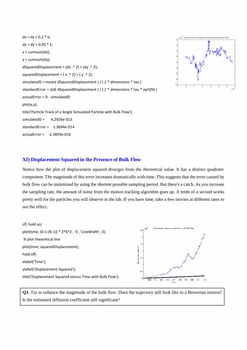
dx = dx + 0.2 * k;
dy = dy + 0.05 * k;
x = cumsum(dx);
y = cumsum(dy);
dSquaredDisplacement = (dx .^ 2) + (dy .^ 2);
squaredDisplacement = ( x .^ 2) + ( y .^ 2);
simulatedD = mean( dSquaredDisplacement ) / ( 2 * dimensions * tau )
standardError = std( dSquaredDisplacement ) / ( 2 * dimensions * tau * sqrt(N) )
actualError = D - simulatedD
plot(x,y);
title('Particle Track of a Single Simulated Particle with Bulk Flow');
simulatedD = 4.2926e-013
standardError = 1.3694e-014
actualError = -2.3859e-016
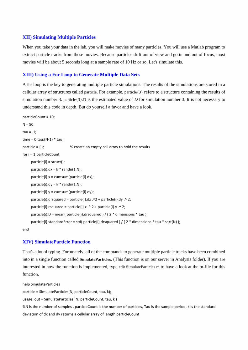
XI) Displacement Squared in the Presence of Bulk Flow
Notice how the plot of displacement squared diverges from the theoretical value. It has a distinct quadratic
component. The magnitude of this error increases dramatically with time. This suggests that the error caused by
bulk flow can be minimized by using the shortest possible sampling period. But there's a catch. As you increase
the sampling rate, the amount of noise from the motion tracking algorithm goes up. A tenth of a second works
pretty well for the particles you will observe in the lab. If you have time, take a few movies at different rates to
see the effect.
clf; hold on;
plot(time, (0:1:(N-1)) * 2*k^2 , 'k', 'LineWidth', 3);
% plot theoretical line
plot(time, squaredDisplacement);
hold off;
xlabel('Time');
ylabel('Displacement Squared');
title('Displacement Squared versus Time with Bulk Flow');
Q3. Try to enhance the magnitude of the bulk flow. Does the trajectory still look like to a Brownian motion?
Is the estimated diffusion coefficient still significant?
XII) Simulating Multiple Particles
When you take your data in the lab, you will make movies of many particles. You will use a Matlab program to
extract particle tracks from these movies. Because particles drift out of view and go in and out of focus, most
movies will be about 5 seconds long at a sample rate of 10 Hz or so. Let's simulate this.
XIII) Using a For Loop to Generate Multiple Data Sets
A for loop is the key to generating multiple particle simulations. The results of the simulations are stored in a
cellular array of structures called particle. For example, particle{3} refers to a structure containing the results of
simulation number 3. particle{3}.D is the estimated value of D for simulation number 3. It is not necessary to
understand this code in depth. But do yourself a favor and have a look.
particleCount = 10;
N = 50;
tau = .1;
time = 0:tau:(N-1) * tau;
particle = { }; % create an empty cell array to hold the results
for i = 1:particleCount
particle{i} = struct();
particle{i}.dx = k * randn(1,N);
particle{i}.x = cumsum(particle{i}.dx);
particle{i}.dy = k * randn(1,N);
particle{i}.y = cumsum(particle{i}.dy);
particle{i}.drsquared = particle{i}.dx .^2 + particle{i}.dy .^ 2;
particle{i}.rsquared = particle{i}.x .^ 2 + particle{i}.y .^ 2;
particle{i}.D = mean( particle{i}.drsquared ) / ( 2 * dimensions * tau );
particle{i}.standardError = std( particle{i}.drsquared ) / ( 2 * dimensions * tau * sqrt(N) );
end
XIV) SimulateParticle Function
That's a lot of typing. Fortunately, all of the commands to generate multiple particle tracks have been combined
into in a single function called SimulateParticles. (This function is on our server in Analysis folder). If you are
interested in how the function is implemented, type edit SimulateParticles.m to have a look at the m-file for this
function.
help SimulateParticles
particle = SimulateParticles(N, particleCount, tau, k);
usage: out = SimulateParticles( N, particleCount, tau, k )
%N is the number of samples , particleCount is the number of particles, Tau is the sample period, k is the standard
deviation of dx and dy returns a cellular array of length particleCount
XV) Look at the Results
The following code plots all of the generated particle tracks on a single set of axes, each in a random color.
clf; hold on;
for i = 1:particleCount
plot(particle{i}.x, particle{i}.y, 'color', rand(1,3));
end
xlabel('X position (m)');
ylabel('Y position (m)');
title('Combined Particle Tracks'); hold off;
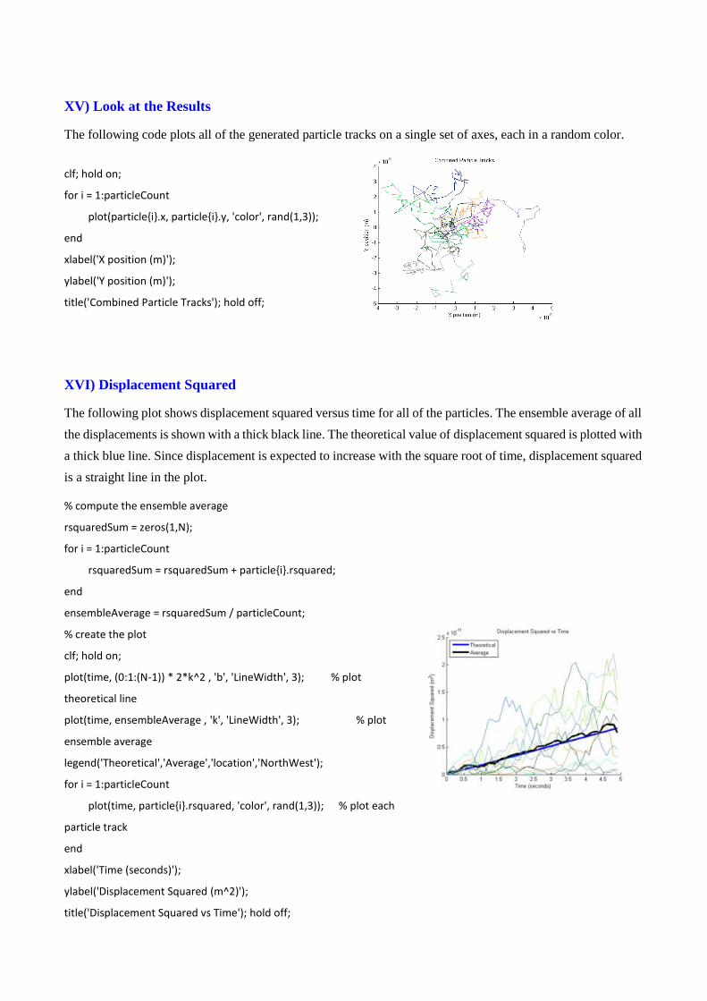
XVI) Displacement Squared
The following plot shows displacement squared versus time for all of the particles. The ensemble average of all
the displacements is shown with a thick black line. The theoretical value of displacement squared is plotted with
a thick blue line. Since displacement is expected to increase with the square root of time, displacement squared
is a straight line in the plot.
% compute the ensemble average
rsquaredSum = zeros(1,N);
for i = 1:particleCount
rsquaredSum = rsquaredSum + particle{i}.rsquared;
end
ensembleAverage = rsquaredSum / particleCount;
% create the plot
clf; hold on;
plot(time, (0:1:(N-1)) * 2*k^2 , 'b', 'LineWidth', 3); % plot
theoretical line
plot(time, ensembleAverage , 'k', 'LineWidth', 3); % plot
ensemble average
legend('Theoretical','Average','location','NorthWest');
for i = 1:particleCount
plot(time, particle{i}.rsquared, 'color', rand(1,3)); % plot each
particle track
end
xlabel('Time (seconds)');
ylabel('Displacement Squared (m^2)');
title('Displacement Squared vs Time'); hold off;
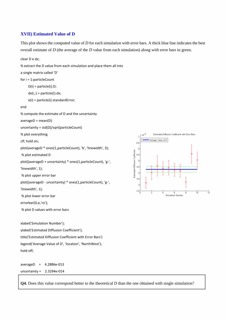
XVII) Estimated Value of D
This plot shows the computed value of D for each simulation with error bars. A thick blue line indicates the best
overall estimate of D (the average of the D value from each simulation) along with error bars in green.
clear D e dx;
% extract the D value from each simulation and place them all into
a single matrix called 'D'
for i = 1:particleCount
D(i) = particle{i}.D;
dx(i,:) = particle{i}.dx;
e(i) = particle{i}.standardError;
end
% compute the estimate of D and the uncertainty
averageD = mean(D)
uncertainty = std(D)/sqrt(particleCount)
% plot everything
clf; hold on;
plot(averageD * ones(1,particleCount), 'b', 'linewidth', 3);
% plot estimated D
plot((averageD + uncertainty) * ones(1,particleCount), 'g-',
'linewidth', 1);
% plot upper error bar
plot((averageD - uncertainty) * ones(1,particleCount), 'g-',
'linewidth', 1);
% plot lower error bar
errorbar(D,e,'ro');
% plot D values with error bars
xlabel('Simulation Number');
ylabel('Estimated Diffusion Coefficient');
title('Estimated Diffusion Coefficient with Error Bars')
legend('Average Value of D', 'location', 'NorthWest');
hold off;
averageD = 4.2886e-013
uncertainty = 2.3294e-014
Q4. Does this value correspond better to the theoretical D than the one obtained with single simulation?
XVIII) Fancy Statistics and Plots
This section looks at the statistical properties of the simulated data in more detail. In particular, it discusses:
Uncertainty in the estimate of the mean value of a random variable from a population of samples
The effect of squaring a normally distributed random variable
The assumption of statistical independence of samples
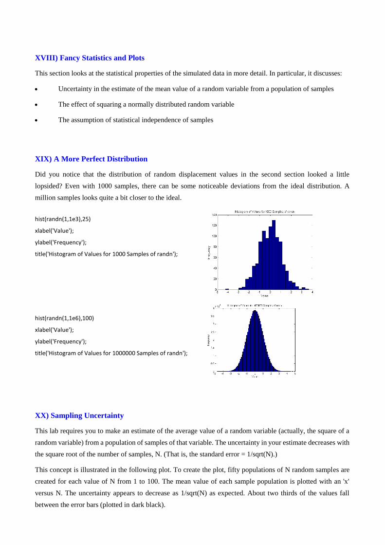
XIX) A More Perfect Distribution
Did you notice that the distribution of random displacement values in the second section looked a little
lopsided? Even with 1000 samples, there can be some noticeable deviations from the ideal distribution. A
million samples looks quite a bit closer to the ideal.
hist(randn(1,1e3),25)
xlabel('Value');
ylabel('Frequency');
title('Histogram of Values for 1000 Samples of randn');
hist(randn(1,1e6),100)
xlabel('Value');
ylabel('Frequency');
title('Histogram of Values for 1000000 Samples of randn');
XX) Sampling Uncertainty
This lab requires you to make an estimate of the average value of a random variable (actually, the square of a
random variable) from a population of samples of that variable. The uncertainty in your estimate decreases with
the square root of the number of samples, N. (That is, the standard error = 1/sqrt(N).)
This concept is illustrated in the following plot. To create the plot, fifty populations of N random samples are
created for each value of N from 1 to 100. The mean value of each sample population is plotted with an 'x'
versus N. The uncertainty appears to decrease as 1/sqrt(N) as expected. About two thirds of the values fall
between the error bars (plotted in dark black).
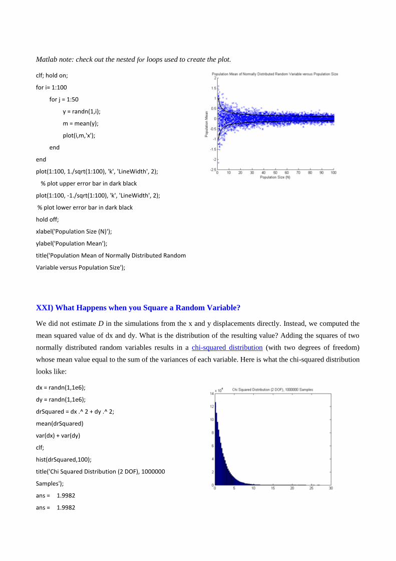
Matlab note: check out the nested for loops used to create the plot.
clf; hold on;
for i= 1:100
for j = 1:50
y = randn(1,i);
m = mean(y);
plot(i,m,'x');
end
end
plot(1:100, 1./sqrt(1:100), 'k', 'LineWidth', 2);
% plot upper error bar in dark black
plot(1:100, -1./sqrt(1:100), 'k', 'LineWidth', 2);
% plot lower error bar in dark black
hold off;
xlabel('Population Size (N)');
ylabel('Population Mean');
title('Population Mean of Normally Distributed Random
Variable versus Population Size');
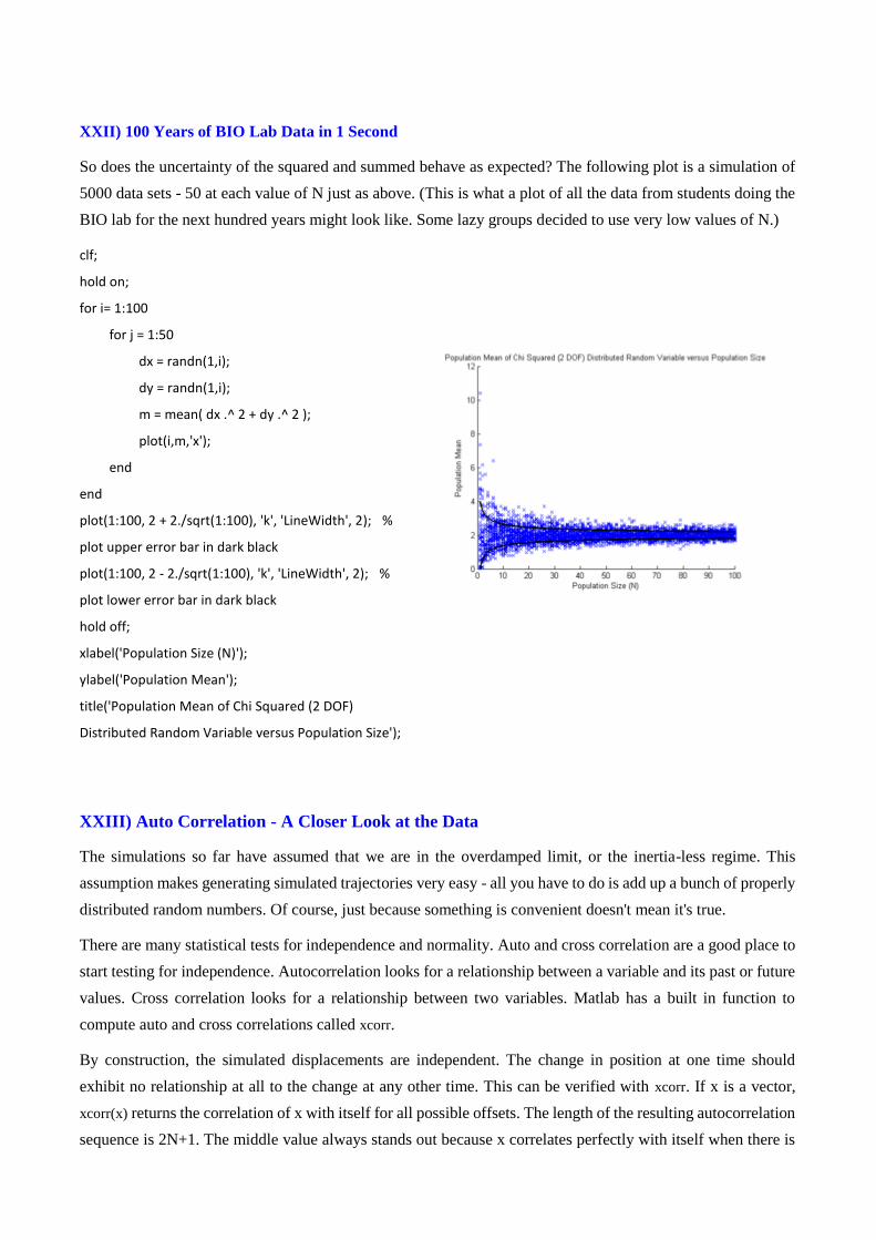
XXI) What Happens when you Square a Random Variable?
We did not estimate D in the simulations from the x and y displacements directly. Instead, we computed the
mean squared value of dx and dy. What is the distribution of the resulting value? Adding the squares of two
normally distributed random variables results in a chi-squared distribution (with two degrees of freedom)
whose mean value equal to the sum of the variances of each variable. Here is what the chi-squared distribution
looks like:
dx = randn(1,1e6);
dy = randn(1,1e6);
drSquared = dx .^ 2 + dy .^ 2;
mean(drSquared)
var(dx) + var(dy)
clf;
hist(drSquared,100);
title('Chi Squared Distribution (2 DOF), 1000000
Samples');
ans = 1.9982
ans = 1.9982
XXII) 100 Years of BIO Lab Data in 1 Second
So does the uncertainty of the squared and summed behave as expected? The following plot is a simulation of
5000 data sets - 50 at each value of N just as above. (This is what a plot of all the data from students doing the
BIO lab for the next hundred years might look like. Some lazy groups decided to use very low values of N.)
clf;
hold on;
for i= 1:100
for j = 1:50
dx = randn(1,i);
dy = randn(1,i);
m = mean( dx .^ 2 + dy .^ 2 );
plot(i,m,'x');
end
end
plot(1:100, 2 + 2./sqrt(1:100), 'k', 'LineWidth', 2); %
plot upper error bar in dark black
plot(1:100, 2 - 2./sqrt(1:100), 'k', 'LineWidth', 2); %
plot lower error bar in dark black
hold off;
xlabel('Population Size (N)');
ylabel('Population Mean');
title('Population Mean of Chi Squared (2 DOF)
Distributed Random Variable versus Population Size');
XXIII) Auto Correlation - A Closer Look at the Data
The simulations so far have assumed that we are in the overdamped limit, or the inertia-less regime. This
assumption makes generating simulated trajectories very easy - all you have to do is add up a bunch of properly
distributed random numbers. Of course, just because something is convenient doesn't mean it's true.
There are many statistical tests for independence and normality. Auto and cross correlation are a good place to
start testing for independence. Autocorrelation looks for a relationship between a variable and its past or future
values. Cross correlation looks for a relationship between two variables. Matlab has a built in function to
compute auto and cross correlations called xcorr.
By construction, the simulated displacements are independent. The change in position at one time should
exhibit no relationship at all to the change at any other time. This can be verified with xcorr. If x is a vector,
xcorr(x) returns the correlation of x with itself for all possible offsets. The length of the resulting autocorrelation
sequence is 2N+1. The middle value always stands out because x correlates perfectly with itself when there is
no offset. Specifying the option 'coeff' causes the xcorr function to normalize this value to exactly 1 --perfect
correlation.
Also notice that the autocorrelation sequence is symmetric about the origin.
clf;
c = xcorr(particle{1}.dx, 'coeff');
xaxis = (1-length(c))/2:1:(length(c)-1)/2;
plot(xaxis, c);
xlabel('Lag');
ylabel('Correlation');
title('Particle 1 x-axis Displacement Autocorrelation');
XIV) Cross Correlation
With two vector arguments, xcorr(x,y) returns a cross correlation matrix. The cross correlation can be used to
test the relationship (or lack thereof) between one particle's trajectory and another's. If two particles move
independently, the cross correlations should be very small. The code below computes the cross correlation
between the x displacements of particle simulations number 1 and 2.
clf;
c = xcorr(particle{1}.dx, particle {2}.dx, 'coeff');
xaxis = (1-length(c))/2:1:(length(c)-1)/2;
plot(xaxis, c);
xlabel('Lag');
ylabel('Correlation');
Title('Particle 1, 2 x-axis Displacement Cross
Correlation');
Q5. The correlation function might be powerful tool to check if a motion corresponds to a Brownian motion.
By the way, you will use this function during the analysis session. How do you judge a motion Brownian or not
using this latter?
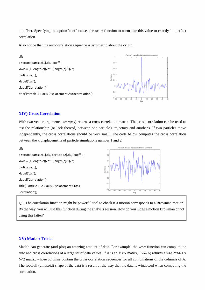
XV) Matlab Tricks
Matlab can generate (and plot) an amazing amount of data. For example, the xcorr function can compute the
auto and cross correlations of a large set of data values. If A is an MxN matrix, xcorr(A) returns a size 2*M-1 x
N^2 matrix whose columns contain the cross-correlation sequences for all combinations of the columns of A.
The football (ellipsoid) shape of the data is a result of the way that the data is windowed when computing the
correlation.
%create an array whose columns contain the dx for each particle
for i = 1:particleCount
allDx(:,i) = particle{i}.dx';
end
% compute all possible auto and cross correlations
c = xcorr(allDx, 'coeff');
% plot the results
clf; hold on;
for i=1:size(c,1)
plot(xaxis, c(:,i),'color',rand(1,3));
end
hold off;
xlabel('Lag');
ylabel('Correlation Coefficient');
title('All Possible Auto and Cross Correlations in the x Dimension');
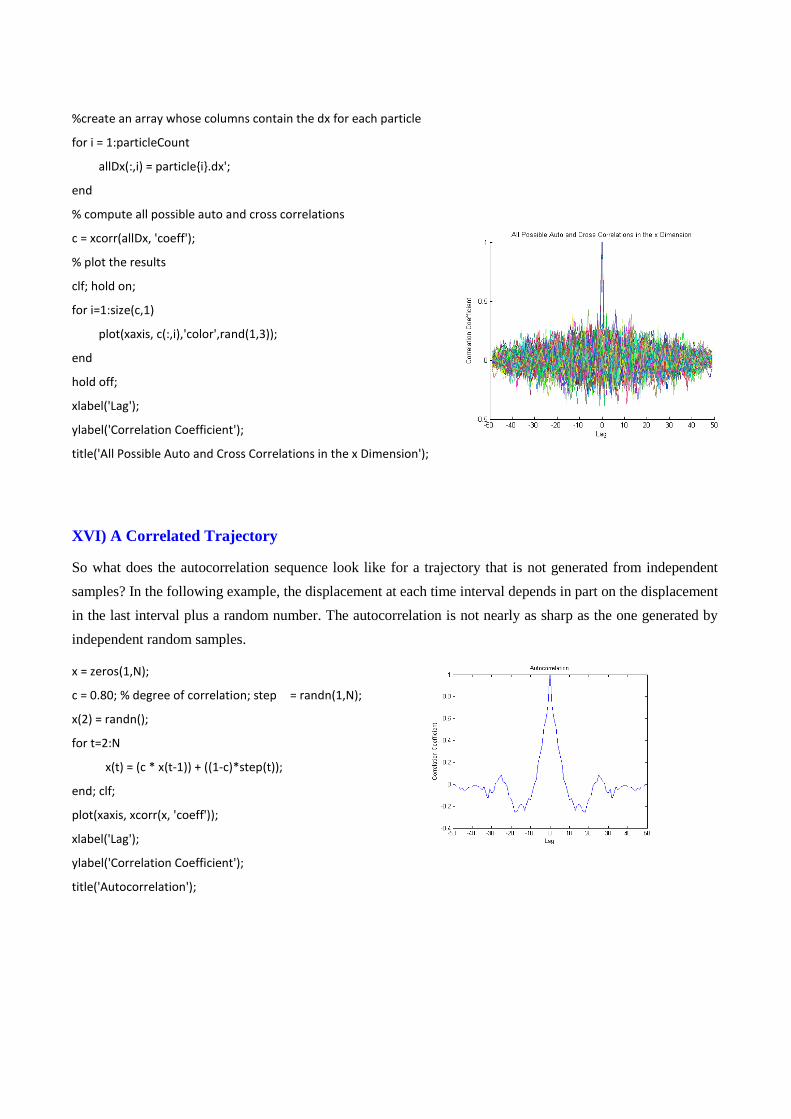
XVI) A Correlated Trajectory
So what does the autocorrelation sequence look like for a trajectory that is not generated from independent
samples? In the following example, the displacement at each time interval depends in part on the displacement
in the last interval plus a random number. The autocorrelation is not nearly as sharp as the one generated by
independent random samples.
x = zeros(1,N);
c = 0.80; % degree of correlation; step = randn(1,N);
x(2) = randn();
for t=2:N
x(t) = (c * x(t-1)) + ((1-c)*step(t));
end; clf;
plot(xaxis, xcorr(x, 'coeff'));
xlabel('Lag');
ylabel('Correlation Coefficient');
title('Autocorrelation');