Simulating Annealing Speed and Current Controllers ......Simulating Annealing Speed and Current...
17
Simulating Annealing Speed and Current Controllers Optimization for PMBLDC Motor Drive Systems MAAD SHATNAWI 1* and EHAB BAYOUMI 2 1 Department of Electrical Engineering Technology, Higher Colleges of Technology, Abu Dhabi, UAE 2 Department of Power Electronics and Energy conversion, Electronics Research Institute, Cairo, EGYPT * Corresponding Author’s Email: [email protected] Abstract: - Brushless Direct Current (BLDC) motors have several advantages including high efficiency and high speed ranges and accordingly are commonly used in a broad range of industrial applications. To accommodate the high performance requirement of the modern industry, optimization of the proportional-integral (PI) and proportional-integral-derivative (PID) controller parameters are highly explored and several tuning methods have been suggested. This work demonstrates a robust permanent magnet brushless dc motor (PMBLDCM) controller design method where a simulated annealing algorithm is employed to tune the parameters of a PI current controller and a PID speed controller of the motor. Three response performance parameters including overshoot, rise time, and settling time are simultaneously optimized during the tuning process. To enhance the overall performance of the system under wide loading conditions, a set of operating points is considered within the objective function. The technique is compared to both Particle Swarm Optimization and Ziegler-Nichols tuning methods and results show the superiority of the proposed approach. Key-Words: - Simulated annealing, multiobjective optimization, PID controller, brushless dc motor, PMBLDCM. 1 Introduction Brushless Direct Current (BLDC) motors are characterized by their high power-savings, long operating life, noiseless operation, high speed ranges, high power-to-weight ratio and high efficiency, and therefore, they are commonly used in a wide range of applications including aerospace, automotive, medical, automation and instrumentation equipment [1-9]. The proportional-integral (PI) and proportional-integral- derivative (PID) controllers are intensely studied in various research papers. These controllers start their attractiveness since the classic Ziegler-Nichols method [10] was presented. There are a variety of tuning approaches proposed to adapt the exceptional requirement of contemporary industry optimization to the PID parameters such as, gain and phase margin method [11], the internal model control (IMC) based PID tuning method [12, 13] and decay ratio method [14]. Moreover, with the recognition of the interior point technique many PID design approaches using Linear Matrix Inequality (LMI) were recommended for the continuous-time systems [15, 16]. Furthermore, PID parameters fine- tuning with state –feedback linear quadratic regulator (LQR) is given in [17]. Evolutionary computations with stochastic search techniques are more capable approach to solve the controller parameters estimation problem. The evolutionary computation for controller parameters identification is applied on BLDC motor drive system. Genetic algorithm (GA) is used to identify the controller parameters of the motor [18]. An evolutionary algorithm based on Particle Swarm Optimization (PSO) with weighting factors has also been introduced and tested on induction motor [19]. In [20] a PSO algorithm with constriction factor is proposed to recognize the controller parameters of the BLDC motor where the controllers’ parameters are tuned to attain a deed beat maximum over index only. It should be noted that even the most successful nature-inspired optimization techniques, such as GA and PSO are also sensitive to the increase of the problem complexity and dimensionality, due to their stochastic nature [21]. In last decade, more attention is given to bacterial foraging optimization (BFO) which has a rich source of potential engineering applications and computation. A few models have been obtained to represent bacterial foraging behaviors and applied it for solving practical problems [22]. Among them, BFO is a population- based numerical optimization algorithm. It solved these engineering problems successfully. But, in complex optimization problems the original BFO algorithm reveals a slow convergence behavior and its performance also heavily decreases with the growth of the search space dimensionality [23]. This paper introduces a robust design approach for PMBLDCM drive current and speed controllers where a Simulated Annealing algorithm is employed to tune WSEAS TRANSACTIONS on COMPUTER RESEARCH Maad Shatnawi, Ehab Bayoumi E-ISSN: 2415-1521 107 Volume 7, 2019
Transcript of Simulating Annealing Speed and Current Controllers ......Simulating Annealing Speed and Current...

Simulating Annealing Speed and Current Controllers Optimization for
PMBLDC Motor Drive Systems
MAAD SHATNAWI1* and EHAB BAYOUMI2 1Department of Electrical Engineering Technology, Higher Colleges of Technology, Abu Dhabi, UAE
2Department of Power Electronics and Energy conversion, Electronics Research Institute, Cairo,
EGYPT *Corresponding Author’s Email: [email protected]
Abstract: - Brushless Direct Current (BLDC) motors have several advantages including high efficiency and high
speed ranges and accordingly are commonly used in a broad range of industrial applications. To accommodate
the high performance requirement of the modern industry, optimization of the proportional-integral (PI) and
proportional-integral-derivative (PID) controller parameters are highly explored and several tuning methods have
been suggested. This work demonstrates a robust permanent magnet brushless dc motor (PMBLDCM) controller
design method where a simulated annealing algorithm is employed to tune the parameters of a PI current
controller and a PID speed controller of the motor. Three response performance parameters including overshoot,
rise time, and settling time are simultaneously optimized during the tuning process. To enhance the overall
performance of the system under wide loading conditions, a set of operating points is considered within the
objective function. The technique is compared to both Particle Swarm Optimization and Ziegler-Nichols tuning
methods and results show the superiority of the proposed approach.
Key-Words: - Simulated annealing, multiobjective optimization, PID controller, brushless dc motor, PMBLDCM.
1 Introduction Brushless Direct Current (BLDC) motors are
characterized by their high power-savings, long
operating life, noiseless operation, high speed ranges,
high power-to-weight ratio and high efficiency, and
therefore, they are commonly used in a wide range of
applications including aerospace, automotive, medical,
automation and instrumentation equipment [1-9]. The
proportional-integral (PI) and proportional-integral-
derivative (PID) controllers are intensely studied in
various research papers. These controllers start their
attractiveness since the classic Ziegler-Nichols method
[10] was presented. There are a variety of tuning approaches proposed to
adapt the exceptional requirement of contemporary
industry optimization to the PID parameters such as,
gain and phase margin method [11], the internal model
control (IMC) based PID tuning method [12, 13] and
decay ratio method [14]. Moreover, with the
recognition of the interior point technique many PID
design approaches using Linear Matrix Inequality
(LMI) were recommended for the continuous-time
systems [15, 16]. Furthermore, PID parameters fine-
tuning with state –feedback linear quadratic regulator
(LQR) is given in [17].
Evolutionary computations with stochastic search
techniques are more capable approach to solve the
controller parameters estimation problem. The
evolutionary computation for controller parameters
identification is applied on BLDC motor drive system.
Genetic algorithm (GA) is used to identify the controller
parameters of the motor [18]. An evolutionary
algorithm based on Particle Swarm Optimization (PSO)
with weighting factors has also been introduced and
tested on induction motor [19]. In [20] a PSO algorithm
with constriction factor is proposed to recognize the
controller parameters of the BLDC motor where the
controllers’ parameters are tuned to attain a deed beat
maximum over index only. It should be noted that even
the most successful nature-inspired optimization
techniques, such as GA and PSO are also sensitive to
the increase of the problem complexity and
dimensionality, due to their stochastic nature [21]. In
last decade, more attention is given to bacterial foraging
optimization (BFO) which has a rich source of potential
engineering applications and computation. A few
models have been obtained to represent bacterial
foraging behaviors and applied it for solving practical
problems [22]. Among them, BFO is a population-
based numerical optimization algorithm. It solved these
engineering problems successfully. But, in complex
optimization problems the original BFO algorithm
reveals a slow convergence behavior and its
performance also heavily decreases with the growth of
the search space dimensionality [23].
This paper introduces a robust design approach for
PMBLDCM drive current and speed controllers where
a Simulated Annealing algorithm is employed to tune
WSEAS TRANSACTIONS on COMPUTER RESEARCH Maad Shatnawi, Ehab Bayoumi
E-ISSN: 2415-1521 107 Volume 7, 2019

the parameters of PID/PI controllers. The maximum
overshoot, rise time and settling time are all
simultaneously minimized within the tuning process.
The proposed algorithm is evaluated and compared with
both the Particle Swarm optimization and Ziegler-
Nichols tuning technique.
This paper is organized as follows. Section 2
introduces the overall block diagram of PMBLDCM
drive system. Section 3 presents the PI/PID controllers
optimization with minimal overshoot, rise time, and
settling using SI technique. The results of the proposed
approach are presented in Section 4. Section 5 provides
some conclusion remarks on the proposed approach for
controlling PMBLDCM drive system.
2 PMBLDCM DRIVE SYSTEM The mathematical model of PMBLDCM drive is given
in [20, 24]. The overall block diagram of the drive
system is given in Fig. 1 where
Rs : stator resistance per phase.
Ls : stator inductance per phase.
e : stator voltage per phase.
m : rotor speed.
vs : stator voltage.
is : staor current.
Te : electromagnetic torque.
TL : load torque.
KT : load torque constant.
Kb : flux constant (volt/rad/sec).
B : motor friction.
J : moment of inertia of PMBLDCM.
3 Simulated Annealing Simulated Annealing (SA) is an effective optimization
technique introduced by Kirkpatrick et al. [25] as a
computational analogous to the annealing process
which is the heating and controlled cooling of a metal
to increase the size of its crystals and reduce their
defects. The function to be optimized in SA is called the
energy, E(x), of the state x, and during that, a parameter
T, the computational temperature, is lowered
throughout the process. SA is an iterative trajectory
descent algorithm that keeps a single candidate solution
at any time [26, 27].
The major advantage of SA is its ability to avoid
being trapped in local optima. This is because the
algorithm applies a random search which does not only
accept changes that improve the objective function, but
also some changes that temporarily worsen it [28, 29].
Geman and Geman [30] presented evidence that
simulated annealing guarantees to converge to the
global optimum if the cooling schedule is adequately
slow. On the other hand, [31, 32] reported through
experience that SA shows a very effective optimization
performance even with relatively rapid cooling
schedules [33]. SA is commonly found in industry and
provides good results [26, 27]. SA have been examined
and showed a well performance in a variety of single-
objective and multiobjective optimization applications
as reported by several researchers. Some of these
applications are wireless telecommunications networks
[27, 32, 34], nurse scheduling problems [35], high-
dimensional and complex nanophotonic engineering
problems [36], pattern detection in seismograms [37],
gene network model optimization [38], and multiple
biological sequence alignment [39- 41].
Fig. 1 Overall block diagram of proposed control for PMBLDCM drives system.
WSEAS TRANSACTIONS on COMPUTER RESEARCH Maad Shatnawi, Ehab Bayoumi
E-ISSN: 2415-1521 108 Volume 7, 2019

Start
(Δf1 < 0 AND (Δf2 0 AND Δf3 0))
OR (Δf2 < 0 AND (Δf1 0 AND Δf3 0))
OR (Δf3 < 0 AND (Δf1 0 AND Δf2 0))
Accept Transition
Generate a random number r ϵ R(0,1)
Stop
No
Yes
Find the fitness functions:
f1(S0) = overshoot OS(S0),
f2(S0) = rise time RT(S0),
f3(S0) = settling time ST(S0)
Decrease
Temperature: T = α T0
Select initial temperature = T0
Select temperature decay = α
Set iteration k = 0
Set initial state S0 by randomly assigning initial values for
Kp(S0) Ki (S0) and Kd(S0)
Make a transition Tr:
Generate a neighborhood state by randomly
increasing or decreasing Kp, Ki and Kd
S = Tr(S0)
Update fitness functions:
f1(S)= overshoot OS(S),
f2(S = rise time RT(S),
f3(S= settling time ST(S)
Calculate the error:
Δf1 = f1(S) - f1(S0),
Δf2 = f2(S) – f2(S0)
Δf3 = f3 (S) – f3(S0)
r < e(-Δ f/T0) Yes
Stopping criteria is met:
(Δf1 <Δf1min AND Δf2 <Δf2min AND Δf3<Δf3min)
OR
K>Kmax
No
No
Return Kp(S), Ki (S) and Kd(S) as the optimal PID parameter values
Return f1(S), f2(S) and f3(S) as the optimal overshoot, rise time, and settling time, respectively
Increase iteration k = k+1
Yes
Fig. 2 Simulated Annealing for PI/PID Controller Optimization.
WSEAS TRANSACTIONS on COMPUTER RESEARCH Maad Shatnawi, Ehab Bayoumi
E-ISSN: 2415-1521 109 Volume 7, 2019

Fig. 3 The current control loop of PMBLDCM drive system.
We employed the Simulated Annealing (SA)
technique to optimize PI and PID controller parameters.
This is a multiobjective optimization problem where
three parameters of controller step response are
simultaneously minimized. During the optimization
process, SA will accept a transition from state S1 to
another state S2 if S2 dominates S1, that is if S2 is not
worse for all objectives than S1 and entirely better for at
least one objective. In other words, SA will accept a
transition that leads to a decrease in all objectives
(overshoot, rise time and settling time) or a decrease in
one of the objectives if other objectives are not changed.
SA will also accept a transition from state S1 to S2 if S2
does not dominate S1 with a probability of e-Δf/T, where
Δf = f(S2) - f(S), and T is the temperature parameter
which is being reduced over time during the
optimization process in order to decrease the possibility
of accepting such transitions. The proposed
optimization algorithm is illustrated in Fig. 2.
4.1 Current Control of PMBLDCM The block diagram of the current control loop of
PMBLDCM drive system is given in Fig. 3. The PM
BLDCM contains an inner loop due to the back emf.
The current loop will cross this back emf loop, creating
a complexity in the development of the model. The
interactions of these loops can be decoupled by suitable
redrawing the block diagram. The open loop transfer
function of the current control loop is:
)1()()1(
)1(_
sTsLRsTsT
sTKKkG
caari
icrp
loopopencurrent
where,
Kr: Gain of the inverter.
Tr: Time constant of the inverter.
Kc: Gain of the current transducer.
Tc: Time constant of the current transducer.
4.2 Current Controller Optimization The PI current controller transfer function is
sT
ksTksG
i
pip
c
)( (2)
Our objective is to find the optimal PI parameters
that stabilizes the system with minimal overshoot, rise
time, and settling time response over the operating
range. The parameters kp and Ti of the PI controller are
randomly initialized and then SA is applied to optimize
kp and Ti to achieve minimal overshoot, rise time, and
settling time. Fig. 4 shows the values of these fitness
functions during SA iterations.
The optimal kp achieved by SA is 0.932 and the
optimal Ti is 0.001765. The resulting PI controller is
s
ssGPI
001765.0
0.932001645.0)(
(3)
4.3 Speed Control of PMBLDCM The block diagram of the speed control loop of
PMBLDCM drive system is given in Fig. 5. The
PMBLDCM contains three inner loops creating a
complexity in the development of the model. Mason’s
rule is applied to reduce the block diagram as shown in
Fig. 6.
21321
* )(1)(
)(
LLLLL
P
sI
sG
s
m
sys
(4)
where the forward path, loop gins are respectively given
as
)()()1(
)1(
sJBsLRsTsT
sTKKkP
aari
ibrp
(5)
WSEAS TRANSACTIONS on COMPUTER RESEARCH Maad Shatnawi, Ehab Bayoumi
E-ISSN: 2415-1521 110 Volume 7, 2019

(A) Maximum overshoot vs. iterations.
(B) Rise time vs. iterations.
(C) Settling time vs. iterations.
Fig. 4 Maximum overshoot, rise time and settling time for the PI current controller during the
optimization process.
-2
0
2
4
6
8
10
12
14
0 10 20 30 40 50 60 70 80 90 100
Overshoot
0
0.0002
0.0004
0.0006
0.0008
0.001
0.0012
0.0014
0.0016
0.0018
0 10 20 30 40 50 60 70 80 90 100
RiseTime
0
0.001
0.002
0.003
0.004
0.005
0.006
0.007
0 10 20 30 40 50 60 70 80 90 100
SettlingTime
WSEAS TRANSACTIONS on COMPUTER RESEARCH Maad Shatnawi, Ehab Bayoumi
E-ISSN: 2415-1521 111 Volume 7, 2019

Fig. 5 Block diagram of the speed control loop for PMBLDCM.
Fig. 6 Reduced block diagram of the speed control loop for PMBLDCM.
)1()()1(
)1(1
sTsLRsTsT
sTKKkL
caari
icrp
(6)
)(
2sJB
KL T
(7)
)()(
2
3sJBsLR
KL
aa
b
(8)
The open loop transfer function of the speed control
loop is:
)1())(1(
)1(
21321
2
_sTLLLLLsT
sTsTTKPkG
wi
iDiwp
openloopspeed
PID
PIDPIDPIDPID
(9)
where,
Kw: Gain of speed transducer.
Tw: Time constant of speed transducer.
PIDPIDPID Dip TTk ,, : Parameters of the PID controller.
4.4 Speed Controller Optimization The PID speed controller transfer function is
sT
sTsTTksG
i
idips
1)(
2 (10)
The parameters PIDPIDPID Dip TTk and, of the PID
controller are randomly initialized. SA is applied to
optimizePIDPIDPID Dip TTk and, to achieve minimal
overshoot, rise time, and settling time. Figure 6 shows
the values of the fitness functions during the
optimization iterations.
The parameters PIDPIDPID Dip TTk and, of the PID
controller are randomly initialized. SA is applied to
optimizePIDPIDPID Dip TTk and, to achieve minimal
overshoot, rise time, and settling time. Fig. 7 shows the
values of the fitness functions during the optimization
iterations.
The optimal kp achieved by SA is 14.6265, the
optimal Ti is 0.0448, and the optimal Td is
0.0000102553. The resulting PID controller is
s
sssGPID
0448.0
)10448.010596.4(6265.14)(
27
(11)
WSEAS TRANSACTIONS on COMPUTER RESEARCH Maad Shatnawi, Ehab Bayoumi
E-ISSN: 2415-1521 112 Volume 7, 2019

(A) Maximum overshoot vs. iterations.
(B) Rise time vs. iterations.
(C) Settling time vs. iterations.
Fig. 7 Maximum overshoot, rise time and settling time for the PID speed controller during the
optimization process.
-0.2
0
0.2
0.4
0.6
0.8
1
1.2
1.4
0 50 100 150 200 250 300 350 400 450 500
Overshoot
0
0.005
0.01
0.015
0.02
0.025
0.03
0.035
0 50 100 150 200 250 300 350 400 450 500
RiseTime
0
0.01
0.02
0.03
0.04
0.05
0.06
0.07
0 50 100 150 200 250 300 350 400 450 500
SettlingTime
WSEAS TRANSACTIONS on COMPUTER RESEARCH Maad Shatnawi, Ehab Bayoumi
E-ISSN: 2415-1521 113 Volume 7, 2019

6 Results The PI current controller and PID speed controllers are
designed with minimal overshoot, rise time and settling
time using SA optimization technique. In Fig. 8, the PI
controller designed is tested at three loading conditions;
heavy, nominal, and light. These are represented
respectively as 150%, 100% and 50% of armature
resistance Ra. It is shown that, in the worst case, the
maximum overshoot is 7.8% (at Ra=50% of the rated
value).
To evaluate the SA PI controller, we compare it with
both PSO and ZN controllers. The PI current controller
of the PMBLDCM drive system using Ziegler-Nichols
PI tuning technique was designed on the rated armature
resistance (Ra) and then tested on 50% and 150% of Ra.
The transfer function of PI speed controller designed by
Ziegler-Nichols [11] is given by
sx
sG ZNPI 4_
1044.5
67.6003623.0
(12)
where Kp = 6.67 , Ti = 5.44x10⁻⁴ , Ki = 12261.
The transfer function of the PSO PI current
controller designed by [20] is given by
s
ssG PSOPI
0054.0
9816.101063.0)(_
(13)
where Kp = 1.9816 , Ti = 0.0054 , Ki = 24.04x10⁶.
A comparison of the proposed PI current controller
with PSO and ZN controllers response at Ra = 50%,
75%, 100%, and150% of its rated value are given in Fig.
9. Fig. 9 clearly illustrates the outperformance of the
proposed PI current controller over both PSO and ZN
controllers. This indicated that the motor can run with
the proposed PI in safe and secure fashion than the other
two PI technique during transient operations. To
evaluate the effectiveness of the proposed PID speed
controller, its performance is tested at different
armature resistance values and different moment of
inertia J values and then compared with PSO and ZN
PID controllers. In Fig. 10, the PID speed controller is
tested at three armature resistance Ra values; 50%,
100%, 150% of its rated value. Fig. 9 shows that the PID
controller response is not affected by varying the
armature resistance. In Fig. 11, the PID speed controller
is tested at three moment of inertia J values; 50%,
100%, 150% of its rated value.
Fig. 8 PI current controller step response at Ra = 50%, 75%, 100%, and150% of its rated value.
WSEAS TRANSACTIONS on COMPUTER RESEARCH Maad Shatnawi, Ehab Bayoumi
E-ISSN: 2415-1521 114 Volume 7, 2019

(A) Step response at Ra=100%.
(B) Step response at Ra=150%.
(C) Step response at Ra=75%.
WSEAS TRANSACTIONS on COMPUTER RESEARCH Maad Shatnawi, Ehab Bayoumi
E-ISSN: 2415-1521 115 Volume 7, 2019

(D) Step response at Ra=50%.
Fig. 9 PI current controllers step response at Ra = (A) 100%, (B) 150%, (C) 75%, and (D) 50% of its
rated value.
Fig. 10 Proposed PID speed controller step response at Ra = 50%, 100%, 150% of its rated value.
We compare our SA PID controller, with both PSO
and ZN controllers. The transfer function of PID speed
controller designed by Ziegler-Nichols is given by [20]
sx
sxsxsG ZNPID 4
428
_105.4
)1105.4100625.5(8.208)(
(14)
where Kp = 208.8, Ti = 4.5x10- , Ki = 464000, Td =
1.125x10⁻⁴, Kd =0.02349.
The transfer function of the PSO PID speed
controller designed by Bayoumi and Soliman [20] is
given by
s
sssG PSOPID
0569.0
)10569.0013827.0(623.4)(
2
_
(15)
Fig. 12 illustrates the step responses of three PID
speed controllers at the rated values of Ra and J. This
clearly shows the superiority the proposed SI PID
controller over the other two PID controllers in running
the motor with a speed response having 0% overshoot
and minimal rise time and settling time.
The three PID controllers are compared at 50% and
150% of the rated armature resistance. Fig. 13 illustrate
the step responses of the three controllers at 50% of Ra
WSEAS TRANSACTIONS on COMPUTER RESEARCH Maad Shatnawi, Ehab Bayoumi
E-ISSN: 2415-1521 116 Volume 7, 2019

while Fig. 14 illustrate the step responses of the three
controllers at 150% of Ra.
The three PID controllers are then evaluated at 50%
and 150% of the rated moment of inertia J. Fig. 15
illustrate the step responses of the three controllers at
50% of J while Fig. 16 illustrate the step responses of
the three controllers at 150% of J.
3 Conclusion This work proposes a simple yet effective approach for
PI current controller and PID speed controller for a
PMBLDC motor drive system. The controller’s
parameters are optimized to simultaneously minimize
three response parameters indices; maximum-
overshoot, rise time and settling time for each
controller. The tuning process is performed using the
Simulated Annealing optimization technique. The
proposed approach was tested over PMBLDC motor
parameters variations and the results show that the
proposed approach outperforms Particle Swarm
Optimization and Ziegler-Nichols tuning methods.
Fig. 11 Proposed PID speed controller step response at J = 50%, 100%, 150% of its rated value.
(A) Step response of the three PID speed controllers.
WSEAS TRANSACTIONS on COMPUTER RESEARCH Maad Shatnawi, Ehab Bayoumi
E-ISSN: 2415-1521 117 Volume 7, 2019
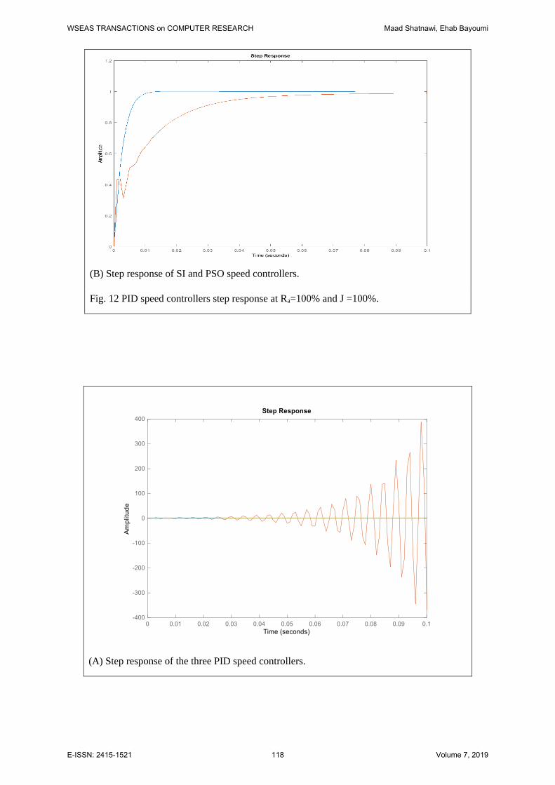
(B) Step response of SI and PSO speed controllers.
Fig. 12 PID speed controllers step response at Ra=100% and J =100%.
(A) Step response of the three PID speed controllers.
WSEAS TRANSACTIONS on COMPUTER RESEARCH Maad Shatnawi, Ehab Bayoumi
E-ISSN: 2415-1521 118 Volume 7, 2019

(B) Step response of SI and PSO speed controllers.
Fig. 13 PID speed controllers step response at Ra=150% and J =100%.
Fig. 14 Step response of the three PID speed controllers step response at Ra=150% and J =100%.
WSEAS TRANSACTIONS on COMPUTER RESEARCH Maad Shatnawi, Ehab Bayoumi
E-ISSN: 2415-1521 119 Volume 7, 2019

(A) Step response of the three PID speed controllers.
(B) Step response of SI and PSO speed controllers.
Fig. 15 PID speed controllers step response at Ra=100% and J =50%.
WSEAS TRANSACTIONS on COMPUTER RESEARCH Maad Shatnawi, Ehab Bayoumi
E-ISSN: 2415-1521 120 Volume 7, 2019

(A) Step response of the three PID speed controllers.
(B) Step response of SI and PSO speed controllers.
Fig. 16 PID speed controllers step response at Ra=100% and J =150%.
WSEAS TRANSACTIONS on COMPUTER RESEARCH Maad Shatnawi, Ehab Bayoumi
E-ISSN: 2415-1521 121 Volume 7, 2019

Appendix
Table 1: The PMBLDCM drive parameters.
Power 373 W
Current 17.35 A
Voltage 160 V
Torque 0.89 N.m
Phase resistance (Ra) 1.4
Phase inductance (La) 2.44 mH
Moment of inertia (J) 0.0002 kg m2
Motor friction (B) 0.002125 N.m/rad/sec
EMF constant (Kb) 0.0513 Vs
Table 2: The converter and transducers parameters.
Converter gain (Kr) 16 V/V
Converter time constant (Tr) 50 µs
Current transducer gain (Kc) 0.288 V/A
Current transducer time constant (Tc) 0.159 ms
Speed transducer gain (Kw) 0.0239 Vs
Speed transducer time constant (Tw) 1ms
References:
[1] C. C. Chan and K. T. Chau, “An Overview of
Power Electronics in Electric Vehicles”, IEEE
Trans. on Ind. Electron., vol. 44, no.1, pp. 3-13,
Feb. 1997.
[2] L. Ben-Brahim y A. Kawamura, “A Fully
Digitized Field-Oriented Controlled Induction
Motor Drive Using Only Current Sensors”, IEEE
Trans. on Ind. Electron., vol. 39, no. 3, pp. 241-
249, June 1992.
[3] Y. Xue, X. Xu, T. G. Habetler y D. M. Divan, “A
Stator Flux-Oriented Voltage Source Variable-
Speed Based on DC Link Measurement,” IEEE
Trans. on Ind. Applicat., vol. 27, no.5, pp. 962-069,
Sept/Oct. 1991.
[4] E.H.E. Bayoumi, “An improved approach of
position and speed sensorless control for
permanent magnet synchronous motor,”
Electromotion Scientofic Journal, vol.14, pp. 81-
90, 2007.
[5] A. R. Millner, “Multi-Hundred Horsepower
Permanent Magnet Brushless Disc Motors,” in
Proc. IEEE APEC Applied Power Electronics
Conference, 1994, pp. 351-355.
[6] P. Pillay, R. Krishnan, “Application
Characteristics of Permanent Magnet Synchronous
and Brushless DC Motors for Servo Drives,” IEEE
Trans. on Ind. Applicat., vol. 27, no.5, pp. 986-996,
Sept/Oct. 1991.
[7] T. Low and M.A. Jabbar, “Permanent-Magnet
Motors for Brushless Operation,” IEEE Trans. on
Ind. Applicat., vol. 26, no.1, pp. 124-129, Jan/Feb
1990.
[8] P.C. Krause, “Analysis of Electric Machinery,”
McGraw-Hill Company, 1987, pp.499-534.
[9] P. Yedamale, “Brushless DC (BLDC) Motor
Fundamentals,” Microship Technology Inc., 2003,
pp.1-20.
[10] Ziegler, J. G., Nichols, N. B., “Optimum settings
for automatic controllers,” Trans. ASME, vol. 62,
pp. 759-768, 1942.
[11] Astrom, K. J. and Hagglund, T., “PID controller,”
2nd Edition, Instrument of Society of America,
Research triangle park, North Carolina, 1995.
[12] Morari, M., and Zafiriou, E., “Robust process
control,” Prentice Hall, USA, 1989.
[13] Rivera, D. E., Morari, M., and Skogestad, S.,
“Internal model control - PID control design”, Ind.
Eng. Chem. Process Des. Dev., 25, pp. 252-265,
1986.
[14] Cohen, G. H. and Coon, G. A., “Theoretical
considerations of retarded control,” Trans. of
ASME, vol. 75, pp. 827, 1953.
[15] Feng, Z., Wang, Q. G. and Lee, T. H., “On the
design of multivariable PID controllers via LMI
approach,” Automatica, vol. 38, pp. 517-526,
2002.
[16] Ge, M., Chiu, M. and Wang, Q. G., “Robust PID
controller design via LMI approach,” J.Process
Control, vol.12, pp. 3-13, 2002.
[17] Ali W.H, Zhang Y, Akujuobi C.M, Tolliver C.L
and Shieh L.S, “DSP-Based PID controller design
for the PMDC motor,” I.J. Modeling and
Simulation, Vol 26, No 2, pp143-150, 2006.
[18] Changliang Xia, PeiJian Guo, Tingna Shi,
Mingehao Wang, “Speed control of brushless DC
motor using genetic algorithm based fuzzy
controller”, 2004 International Conference on
Intelligent Mechatronics and Automation,
Chengdu, China, 26-31 Aug. 2004.
[19] Picardi C., Rogano N., “Parameter Identification of
Induction Motor Based on Particle Swarm
Optimization,” International Symposium on Power
Electronics, Electric Drives, Automation and
Motion, May 23-26, 2006.
WSEAS TRANSACTIONS on COMPUTER RESEARCH Maad Shatnawi, Ehab Bayoumi
E-ISSN: 2415-1521 122 Volume 7, 2019

[20] Ehab H.E. Bayoumi, Hisham M. Soliman, “PID/PI
tuning for minimal overshoot of permanent-
magnet brushless DC motor drive using particle
swarm optimization”, Electromotion Scientific
Journal, Vol. 14, No. 4, pp.: 198-208, 2007.
[21] Kennedy, J. and Eberhart, R.C. Swarm
Intelligence, Morgan Kaufmann, San Francisco,
2001.
[22] Ehab H.E. Bayoumi, “Parameter estimation of
cage induction motors using cooperative bacteria
foraging optimization”, Electromotion Scientific
Journal Vol. 17, No. 4, pp: 247-260, 2010.
[23] El-Abd, M. and Kamel, M., “A taxonomy of
cooperative search algorithms, “Proceedings of the
2nd International Workshop on Hybrid
Metaheuristics, pp.32–41, 2005.
[24] R.Krishnan, “Permanent Magnet Synchronous and
Brushless DC Motor Drives: Theory, Operation,
Performance, Modelling, Simulation, Analysis and
Design, Part 3: Permanent Magnet Brushless DC
Machines and Their Control,” Virginia Tech,
Blacksburg, 2000.
[25] Bhaskara, R. M., de Brevern, A. G., Srinivasan, N.,
2012. Understanding the role of domain-domain
linkers in the spatial orientation of domains in
multi- domain proteins. Journal of Biomolecular
Structure and Dynamics, 1-14.
[26] Vega-Rodriguez, M. A., Gomez-Pulido, J. A.,
Alba, E., Vega-Perez, D., Priem-Mendes, S.,
Molina, G., 2007. Evaluation of different
metaheuristics solving the rnd problem. In:
Applications of Evolutionary Computing.
Springer, pp. 101-110.
[27] Mendes, S. P., Molina, G., Vega-Rodriguez, M. A.,
Gomez-Pulido, J. A., Saez, Y., Miranda, G.,
Segura, C., Alba, E., Isasi, P., Leon, C., et al., 2009.
Bench- marking a wide spectrum of metaheuristic
techniques for the radio network design problem.
Evolutionary Computation, IEEE Transactions on
13 (5), 1133-1150.
[28] Busetti, F., 2003. Simulated annealing overview.
[29] Henderson, D., Jacobson, S. H., Johnson, A. W.,
2003. The theory and practice of simulated
annealing. In: Handbook of metaheuristics.
Springer, pp. 287-319.
[30] Geman, S., Geman, D., 1984. Stochastic
relaxation, gibbs distributions, and the bayesian
restoration of images. Pattern Analysis and
Machine Intelligence, IEEE Transactions on (6),
721-741.
[31] Salamon, P., Sibani, P., Frost, R., 2002. Facts,
conjectures, and improvements for simulated
annealing. SIAM.
[32] Ingber, L., 1993. Simulated annealing: Practice
versus theory. Mathematical and computer
modelling 18 (11), 29-57.
[33] Smith, K. I., Everson, R. M., Fieldsend, J. E.,
Murphy, C., Misra, R., 2008. Dominance-based
multiobjective simulated annealing. Evolutionary
Computation, IEEE Transactions on 12 (3), 323-
342.
[34] Jaraiz-Simon, M. D., Gomez-Pulido, J. A., Vega-
Rodriguez, M. A., Sanchez- Perez, J. M., 2013.
Simulated annealing for real-time vertical-handoff
in wireless networks. In: Advances in
Computational Intelligence. Springer, pp. 198-
209.
[35] Kundu, S., Mahato, M., Mahanty, B., Acharyya,
S., 2008. Comparative performance of simulated
annealing and genetic algorithm in solving nurse
scheduling problem. In: Proceedings of the
International MultiConference of Engineers and
Computer Scientists. Vol. 1.
[36] Bertsimas, D., Nohadani, O., 2010. Robust
optimization with simulated annealing. Journal of
Global Optimization 48 (2), 323-334.
[37] Huang, K.-Y., Hsieh, Y.-H., 2011. Very fast
simulated annealing for pattern detection and
seismic applications. In: Geoscience and Remote
Sensing Symposium (IGARSS), 2011 IEEE
International. IEEE, pp. 499-502.
[38] Tomshine, J., Kaznessis, Y. N., 2006.
Optimization of a stochastically simulated gene
network model via simulated annealing.
Biophysical journal 91 (9), 3196-3205.
[39] Ishikawa, M., Toya, T., Hoshida, M., Nitta, K.,
Ogiwara, A., Kanehisa, M., 1993. Multiple
sequence alignment by parallel simulated
annealing. Computer applications in the
biosciences: CABIOS 9 (3), 267-273.
[40] Kim, J., Pramanik, S., Chung, M. J., 1994.
Multiple sequence alignment using simulated
annealing. Computer applications in the
biosciences: CABIOS 10 (4), 419-426.
[41] Kirkpatrick, S., Jr., D. G., Vecchi, M. P., 1983.
Optimization by simulated annealing. Science 220
(4598), 671-680.
WSEAS TRANSACTIONS on COMPUTER RESEARCH Maad Shatnawi, Ehab Bayoumi
E-ISSN: 2415-1521 123 Volume 7, 2019