Model specifications ABI – Open Knee Data

1. MetadataAuckland Bioengineering InstituteAuckland, New Zealand

Contributors:Thor BesierMarco SchneiderNynke RooksMousa Kazemi

Contact: t.besier@auckland.ac.nz10th of August 2018

2. Data utilization Open Knee Data (NIfTI files)- Left knee, 25 year old female, 1.73 m, 68 kg

To obtain bone and cartilage geometries:- General purpose imaging (MRI) - sagittal 320 images, 480x316 uint16

Not using:- Cartilage imaging (MRI) - sagittal 224 images, 512x448 uint16- Soft tissue imaging - axial plane (MRI) 50 images, 432x512 uint16- Soft tissue imaging - sagittal plane (MRI) 50 images, 512x432 uint16- Soft tissue imaging - coronal plane (MRI) 50 images, 512x432 uint16

1

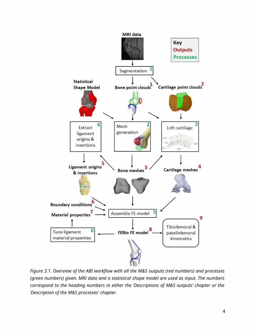
3. OverviewThis document specifies the intended modelling and simulation (M&S) workflow of the Auckland Bioengineering Institute (ABI) to develop a patient specific computational model of the knee (Figure 3.1). The purpose of the model is to simulate passive knee flexion from 0 to 90 degrees to determine the 6 degrees of freedom (DOF) kinematics of the tibiofemoral and patellofemoral joint.

In summary, general purpose sagittal plane MRI data of the knee will be manually segmented using a custom MATLAB script to obtain point clouds of the distal femur, proximal tibia, patella, and proximal fibula, and the articular surfaces of the femoral cartilage, tibial cartilage, and patellar cartilage. A statistical shape model (SSM) will inform the mesh generation of the bone and cartilage from point clouds using custom python scripts. These scripts a put together in a ‘workflow’, which can be run using our Musculoskeletal Atlas Project (MAP) client (referred to hereon as the ‘MAP Client’). Principal component fitting and regression will be used to obtain triangulated meshes of the bones, and the cartilage will be lofted with custom Python code to obtain hexahedral meshes of the cartilage.

The finite element (FE) model will be assembled using custom Python code to be solved using the FEBio solver. The bones will be modelled as rigid bodies and the cartilage modelled as nearly incompressible linear elastic materials. Ligament bundles will be modelled as uniaxial non-linear tension only springs between origin and insertion points embedded in the SSM, and the menisci will be modelled as three linear springs each. A constant quadriceps tendon force will be used to stabilize the patella. The femur will be fixed in 6 degrees of freedom, the tibia fixed in flexion only, the fibula tied to the tibia, and the patella will be unconstrained. Cartilage will be tied to their corresponding bones, and cartilage-cartilage contact will be modelled as frictionless facet-on-facet sliding. The anatomical coordinate systems of the knee model for obtaining the simulated kinematics will be based on those reported by Grood and Suntay (1983) and will be extracted from the SSM using anatomical landmarks (Zhang et al., 2016).

A Python optimisation script will be used to tune the ligament force-displacement properties to literature laxity profiles of the entire knee. Post-optimisation, passive knee flexion kinematics from 0 to 90 degrees will be obtained by simulating knee contact at increments of 10 degrees by prescribing tibia flexion-extension angle relative to the femur.

2

Figure 3.1. Overview of the ABI workflow with all the M&S outputs (red numbers) and processes (green numbers) given. MRI data and a statistical shape model are used as input. The numbers correspond to the heading numbers in either the ‘Descriptions of M&S outputs’ chapter or the ‘Description of the M&S processes’ chapter.

3

4. Modelling and Simulation Outputs The sections below provide descriptions of the target modelling and simulation outputs expected to be obtained from this workflow.

4.1 Bone point clouds (femur, tibia, fibula, and patella)X, Y and Z coordinates of segmented points for the femur, tibia, fibula, and patella bone geometries. Coordinates will be in scanner coordinate system (converted to mm using imaging information) and stored in a text file (.pts) (e.g. Femur_bone_points.pts, Tibia_bone_points.pts, etc).

4.2 Cartilage point clouds (femur, tibia, and patellar cartilage surfaces)X, Y and Z coordinates of segmented points for the femoral, medial tibial, lateral tibial, and patellar cartilage geometries (articulating surface of the cartilage only, as the subchondral surface is segmented in 4.1). Coordinates will be in scanner coordinate system (mm) and stored in a text file (.pts). (e.g. Femur_cartilage_points.pts, Tibia_cartilage_points.pts, etc.)

4.3 Bone meshes (femur, tibia, fibula, patella)Meshes for the femur, tibia, fibula, and patella composed of triangular shell elements (3 nodes per element). Meshes will be stored as an .asc file (containing nodal coordinates and connectivity).

4.4 Cartilage meshes (femur, tibia, fibula, patella)Meshes of the femoral, medial tibial, lateral tibial, and patellar cartilage composed of solid hexahedral elements (8 nodes per element). The cartilage meshes will be exported in .asc files (containing nodal coordinates and connectivity).

Table 4.5.1. Ligament, menisci, tendon, and joint capsule structures that will be included in the FE model

Tibiofemoral joint Patellofemoral joint

Anterior cruciate ligament (ACL) Patellar tendon (PT)

Posterior cruciate ligament (PCL) Lateral patellofemoral ligament (LPFL)

Lateral collateral ligament (LCL) Medial patellofemoral ligament (MPFL)

Medial collateral ligament (MCL) Quadriceps tendon (QT) (Force vectors)

Popliteofibular ligament (PFL)

Oblique popliteal ligament (OPL)

Medial posterior capsule (mPCAP)

Lateral posterior capsule (lPCAP)

Medial and lateral meniscus (mMen & lMen)

4

4.5 Ligament origin & insertion locationNode numbers and coordinates (X,Y,Z) on the bone meshes describing ligament origins and insertion points. The ligaments, menisci, tendon and joint capsule structures to be included are shown in Table 4.5.1. The number of spring elements to be modelled per ligament (bundle) is shown in Table 4.5.2.

Table 4.5.2. Number of spring elements per ligament bundle. Anteromedial ACL (amACL), Posterolateral ACL (plACL), Posteromedial PCL (pmPCL), Anterolateral PCL (alPCL), Superficial MCL (sMCL), Posterior deep MCL (pdMCL), Medial posterior capsule (mPCAP), Lateral posterior capsule (lPCAP), Medial meniscus (mMen), Lateral meniscus (lMen).

Ligament Bundles Number of elements

ACL amACL 3

plACL 3

PCL pmPCL 3

alPCL 3

MCL sMCL 6

pdMCL 3

LCL 5

OPL 3

PFL 3

pCAP mPCAP 14

lPCAP 14

Men mMen 3

lMen 3

MPFL 5

LPFL 5

PT 5

5

4.6 Boundary conditionsThe boundary conditions to be used in the FE analysis for calculating joint kinematics.

Bone (rigid bodies) constraintsFemur: Fixed in 6 DOFTibia: Fixed in 1 DOF (flexion and extension), free in remaining 5 DOF Fibula: Tied to the tibiaPatella: Free in 6 DOF (unconstrained)

Contact constraintsCartilage-Bone: Tied contactCartilage-Cartilage: Frictionless facet-on-facet sliding

Applied forces Patella: Constant passive quadriceps force vectors used to stabilize the patella during simulations by acting on the patella bone mesh. Quadriceps force will be split into three separate force vectors similar to (Mesfar and Shirazi-Adl, 2005):

- Vastus medialis obliquus (VMO) vector: 10N * [- sin(41° ), sin(0° ), cos(41° )]- Rectus femoris/vastus intermedius medialis (RF/VIM): 25N * [sin(0° ), sin(4° ), cos (0° )]- Vastus lateralis (VL) : 5N * [sin(22° ), sin(0° ), cos(22° )]

4.7 Material properties4.7.1 Bone The femur, tibia, fibula, and patella bones will be modelled as rigid bodies.

4.7.2 Cartilage The femoral, medial tibial, lateral tibial, and patellar cartilage will be modelled as an isotropic, linear elastic, nearly incompressible material (Young's Modulus: 15.0 MPa, Poisson's ratio: 0.475) (Guess et al., 2010; Donahue et al., 2002; Zielinska and Donahue, 2006; Kiapour et al., 2014).

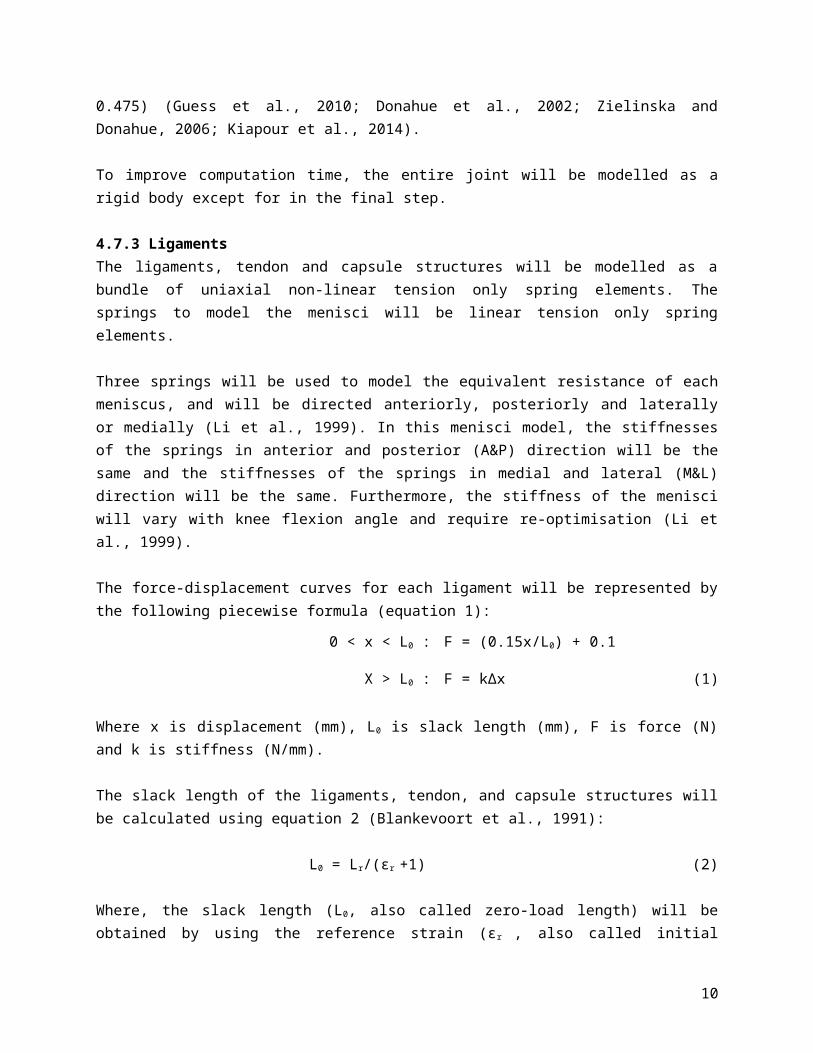
To improve computation time, the entire joint will be modelled as a rigid body except for in the final step. 4.7.3 Ligaments The ligaments, tendon and capsule structures will be modelled as a bundle of uniaxial non-linear tension only spring elements. The springs to model the menisci will be linear tension only spring elements.

Three springs will be used to model the equivalent resistance of each meniscus, and will be directed anteriorly, posteriorly and laterally or medially (Li et al., 1999). In this menisci model, the stiffnesses of the springs in anterior and posterior (A&P) direction will be the same and the stiffnesses of the springs in medial and lateral (M&L) direction will be the same. Furthermore,

6

the stiffness of the menisci will vary with knee flexion angle and require re-optimisation (Li et al., 1999).

The force-displacement curves for each ligament will be represented by the following piecewise formula (equation 1):

0 < x < L0 : F = (0.15x/L0) + 0.1

X > L0 : F = kΔx (1)

Where x is displacement (mm), L0 is slack length (mm), F is force (N) and k is stiffness (N/mm).

The slack length of the ligaments, tendon, and capsule structures will be calculated using equation 2 (Blankevoort et al., 1991):

L0 = Lr/(εr +1) (2)

Where, the slack length (L0, also called zero-load length) will be obtained by using the reference strain (εr , also called initial strain), and the length of the ligament in full extension (L r). Lr will be estimated by calculating the length of the springs at full extension (0 degrees flexion).

The material properties used to obtain the force-displacement curves of the ligaments, menisci, tendon, and capsule structures will be initialised with literature values (Table 4.7.3.1). The ligaments will then be optimised according to anterior-posterior knee laxity profiles (Li et al., 2002) and internal-external rotation profiles (Li et al., 2002).

ACL, PCL, MCL and LCL stiffnesses were obtained by taking the average of ligament stiffness reported in Mommersteeg et al. (1995). In Harris et al. (2016) the final ligament stiffness values of their four calibrated knee models are given. Their stiffness values for the ACL, PCL, MCL and LCL were compared to the stiffness values that will be used as initial values in our model. It was found that for the ACL and PCL their value is lower and for the LCL and MCL their value is higher. For this reason there is chosen to use their average calibrated value as initial value for the OPL, PFL and PCAP.

In literature was found that the calibrated reference strains in knee models differ quite a bit between different knees modeled (Baldwin et al., 2012; Harris et al., 2016; Blankevoort and Huiskes, 1996). Therefore there was chosen to use the average of the calibrated reference strains of four different knees from (Harris et al., 2016) as an initial value for the reference strain for most of the ligaments and capsule structures, to calculate the initial slack length. The average value of the calibrated reference strain was taken and converted (subtracted by 1) to be usable in the slack length formula. For the MPFL, LPFL and PT, no value for the reference strain was found. Therefore there was chosen to calculate the slack length by using 0 reference strain for these structures.

7

Table 4.7.3.1. Initial ligament, menisci, tendon, and capsule structure properties based on literature values.

Number of springs in the model

Stiffness whole structure ± SD (N/mm)

Stiffness k per spring (N/mm)

Reference strain εr ± SD

ACL 6 178 ± 63 (Mommersteeg et al.,

1995)

29.7 amACL: -0.005 ± 0.092(Harris et al., 2016)

plACL: -0.02 0 ± 0.090

(Harris et al., 2016)

PCL 6 213 ± 78 (Mommersteeg et al.,

1995)

35.5 alPCL: -0.048 ± 0.076(Harris et al., 2016)

pmPCL: -0.028 ± 0.080(Harris et al., 2016)

MCL 9 100 ± 13 (Mommersteeg et al.,

1995)

11.1 sMCL: 0.044 ± 0.026 (Harris et al., 2016)

pdMCL: -0.018 ± 0.089 (Harris et al., 2016)

LCL 5 74 ± 28 (Mommersteeg et al., 1995)

14.8 0.015 ± 0.021 (Harris et al., 2016)

MPFL 5 42.5 ± 10.2 (Criscenti et al., 2016)

8.5 0

LPFL 5 16 ± 7 (Merican et al., 2009)

3.2 0

OPL 3 49 ± 19 (Harris et al., 2016)

16.3 -0.085 ± 0.045 (Harris et al., 2016)

PT 5 ~2200 ± 700 (Reeves et al., 2002)

440 0

PFL 3 44 ± 27 (Harris et al., 2016)

14.7 -0.060 ± 0.099 (Harris et al., 2016)

PCAP 28 189 ± 12 (Harris et al., 2016)

6.8 mPCAP: 0.023 ±0.054 (Harris et al., 2016)

lPCAP: 0.043 ± 0.015 (Harris et al., 2016)

Men (linear)

3 medial & 3 lateral

N/A A&P: 8 (full extension), 5 (30 deg. flexion)

(Li et al., 1999)M&L: 7 (full extension),

5 (30 deg. flexion) (Li et al., 1999)

N/A

8

4.8 FEBio FE model The FE model will be assembled with bone and cartilage meshes, loads and boundary conditions, material properties, and ligament spring elements will be created using the ligament origin and insertion points.Ten FEBio (*.feb) files will be created to simulate the quasi static mechanics of the knee from 0 to 90 degrees in the flex/ext axis at 10 degree increments: 0, 10, 20, 30, 40, 50, 60, 70, 80, and 90 degrees. These will be used for calibration purposes.

4.9 Tibiofemoral and patellofemoral kinematics Kinematics (tibia + patella):Graphs of the TF kinematics across 0-90 degrees passive flexion for 6DOF. Graphs of the PF kinematics across 0-90 degrees passive flexion for 6DOF.

Definitions of the movements in the tibiofemoral and patellofemoral joint (fixed femur): Tibia translations (+rotations around same axis): - anterior (+) - posterior (varus - valgus) - medial - lateral (+) (extension - flexion)

- superior (+) - inferior (internal - external)Patella translations (+rotations around same axis): - anterior (+) - posterior (spin)

- medial - lateral (+) (flexion) - superior (+) - inferior (tilt)Directions: Right hand rule

9

5. Modelling and Simulation processes for obtaining target outputsThe sections below provide detailed descriptions of the processes that will be used to obtain target outputs in Section 4.

5.1 Segmentation This section describes how the bone point clouds (Section 4.1) and cartilage point clouds (Section 4.2) will be obtained from the MRI data.

A custom MATLAB script will be used for segmentation. The script allows the user to pick points on each slice of the image stack, which are then used to fit a cubic spline. Once the user has finished with picking points, the cubic splines are sampled to obtain 20 points within each manually segmented point to create a dense point cloud of the segmented object.

Input: NIfTI files. Output: Point clouds of the bones (distal femur, proximal tibia, proximal fibula, patella) and cartilage (femoral cartilage, tibial cartilage, patellar cartilage) exported as .pts files containing x,y,z coordinates in mm.

Procedure:1. Load the image stack using the segment_niftii_GeneralPurpose.m script (for NIfTI

format). 2. The script will prompt the user to select a region of interest for segmentation. The user

will be required to select the top left corner (left-click & hold) and the bottom right corner of this region (release).

3. The selected region will then be displayed to the user. The user will then be able to change which slice they are viewing within this region using the “MR sequence slider”.

4. The script enables the user to segment one of the bones or cartilage structures one slice at a time.* This is done by clicking along the boundaries of the bone/cartilage to create points for a cubic spline. When segmenting cartilage, only the articular surface boundary will be segmented since the subchondral boundary will be segmented with the bone.

5. If a mistake is made, the “Clear frame” button will be pressed to clear the slice, and the slice will be segmented again.

6. The “Save splines” button will re-interpolate the current splines as a point cloud and export the point cloud directly to the “pt_clouds.pts” file.

7. Before continuing to segment another bone/cartilage, the “pt_clouds.pts” file will be renamed to avoid loss of data due to the file being overwritten.

*If multiple contours belonging to the same object are present within the slice, the user must segment one contour first and continue. The additional contours will need to be segmented in a separate MATLAB session after saving and renaming the “pt_clouds.pts” file. The point clouds can be added to the original pts file afterwards by copying and pasting in notepad.

10

11

5.2 Mesh generation This section describes how the bone meshes (Section 4.3) will be obtained from the segmented point clouds (Section 4.1) and a statistical shape model (SSM).

A SSM will be used to generate the bone meshes, inform cartilage boundaries, inform ligament origin and insertions, and define the anatomical coordinate systems (ACS). This will be done using custom python scripts in the MAP client.

Input: Bone point clouds and SSM.Output: Full bone meshes exported as STLs.

Procedure (or steps, as they are referred to in the MAP Client):1. We will rigidly align the SSM of the lower limb (femur, tibia, fibula, and patella) to the

entire segmented point cloud of the knee. 2. We will use the principal components (PC) in conjunction with the patients’ sex, height,

and weight data to perform a partial least squares regression (PLSR) fit of the SSM to the segmented point clouds to obtain an intermediate fitted mesh (Figure 5.2.1).

Figure 5.2.1. Patient specific meshes of the femur, patella, tibia, fibula, femoral cartilage, patellar cartilage, and tibial cartilage overlaid with their corresponding segmented point clouds.

12

3. A local fit will be performed on the intermediate fitted mesh of each bone to each corresponding segmented point cloud to obtain the final fitted meshes.

4. The ACS of each individual bone will be extracted from the fitted SSM, including the proximal-distal axis, medial-lateral axis, and the anterior-posterior axis. The process for extracting the ACSs is detailed in section 5.5.1.

5. The ACS of the femur will be used to rigidly align the entire knee to the origin and axes of the global coordinate system, with the proximal-distal axis aligned with the z-axis, the medial-lateral axis aligned with the x-axis, and the anterior-posterior axis aligned with the y-axis.

6. Meshes will be exported as STL files.

5.3 Loft cartilage In this process the cartilage meshes (Section 4.4) will be obtained by using the bone point clouds (Section 4.1), cartilage point clouds (Section 4.2) and the bone meshes (Section 4.3).

The cartilage subchondral surface nodes were previously embedded as material points in the bone meshes and will be extracted to loft the cartilage mesh using custom python code. This was done by registering the SSM to the OpenKnee model (Erdemir, 2013), and then projecting the cartilage subchondral nodes to the closest nodes on the registered mesh. The patch parametric coordinates (“material points”) of each of these closest nodes was then determined and recorded.

Input: Segmented cartilage point clouds, bone point clouds, and meshes for the femur, tibia, and patella.Output: Meshes of the femoral cartilage, patellar cartilage, and tibial cartilage.

Procedure:1. A custom python code extracts the subchondral cartilage nodes from the pre-aligned

bone mesh using the recorded material points for the femur, tibia, and patella.2. For each subchondral mesh node, the python code finds the closest bone point in the

corresponding bone point cloud using the KDTree algorithm. 3. The python code calculates the surface normal vector of the mesh at the node, and uses

the KDTree algorithm to identify the closest point in the cartilage point cloud that is along the vector projected from the bone point (identified in 2).

4. The cartilage thickness for each mesh node is calculated as the displacement between the bone point and the cartilage point (identified in 2 and 3) along the normal vector. This is repeated for each node in the mesh.

13

Figure 5.3.1. Cartilage lofting process.

5. The subchondral bone mesh nodes are lofted in the direction of the surface normals at each node using the cartilage thickness at each node.

6. Host mesh fitting (HMF) is used to fit a template hexahedral cartilage mesh to the lofted cartilage nodes. This ensures that nodal connectivity is maintained without negative element jacobians being generated following projections.

Figure 5.3.2. Post HMF fitted patient specific mesh.

7. The rigid transforms used to align the bones meshes will be applied to the cartilage meshes.

8. Final hexahedral mesh exported as an *.asc file.

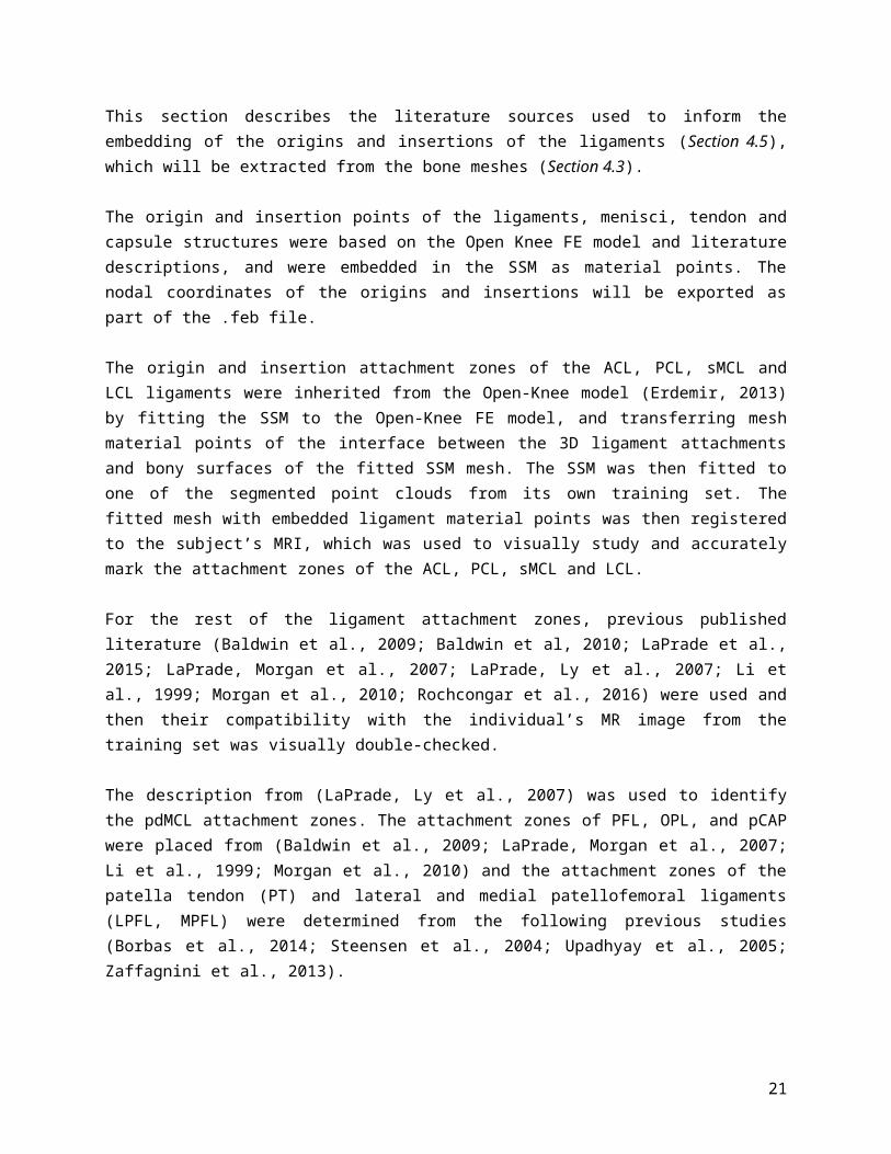
5.4 Extract ligament origins and insertions This section describes the literature sources used to inform the embedding of the origins and insertions of the ligaments (Section 4.5), which will be extracted from the bone meshes (Section 4.3).

The origin and insertion points of the ligaments, menisci, tendon and capsule structures were based on the Open Knee FE model and literature descriptions, and were embedded in the SSM as material points. The nodal coordinates of the origins and insertions will be exported as part of the .feb file.

14

The origin and insertion attachment zones of the ACL, PCL, sMCL and LCL ligaments were inherited from the Open-Knee model (Erdemir, 2013) by fitting the SSM to the Open-Knee FE model, and transferring mesh material points of the interface between the 3D ligament attachments and bony surfaces of the fitted SSM mesh. The SSM was then fitted to one of the segmented point clouds from its own training set. The fitted mesh with embedded ligament material points was then registered to the subject’s MRI, which was used to visually study and accurately mark the attachment zones of the ACL, PCL, sMCL and LCL.

For the rest of the ligament attachment zones, previous published literature (Baldwin et al., 2009; Baldwin et al, 2010; LaPrade et al., 2015; LaPrade, Morgan et al., 2007; LaPrade, Ly et al., 2007; Li et al., 1999; Morgan et al., 2010; Rochcongar et al., 2016) were used and then their compatibility with the individual’s MR image from the training set was visually double-checked.

The description from (LaPrade, Ly et al., 2007) was used to identify the pdMCL attachment zones. The attachment zones of PFL, OPL, and pCAP were placed from (Baldwin et al., 2009; LaPrade, Morgan et al., 2007; Li et al., 1999; Morgan et al., 2010) and the attachment zones of the patella tendon (PT) and lateral and medial patellofemoral ligaments (LPFL, MPFL) were determined from the following previous studies (Borbas et al., 2014; Steensen et al., 2004; Upadhyay et al., 2005; Zaffagnini et al., 2013).

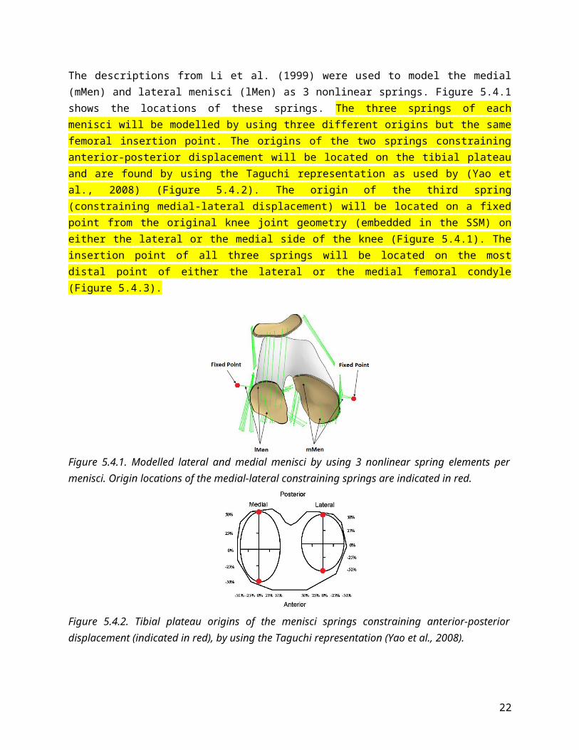
The descriptions from Li et al. (1999) were used to model the medial (mMen) and lateral menisci (lMen) as 3 nonlinear springs. Figure 5.4.1 shows the locations of these springs. The three springs of each menisci will be modelled by using three different origins but the same femoral insertion point. The origins of the two springs constraining anterior-posterior displacement will be located on the tibial plateau and are found by using the Taguchi representation as used by (Yao et al., 2008) (Figure 5.4.2). The origin of the third spring (constraining medial-lateral displacement) will be located on a fixed point from the original knee joint geometry (embedded in the SSM) on either the lateral or the medial side of the knee (Figure 5.4.1). The insertion point of all three springs will be located on the most distal point of either the lateral or the medial femoral condyle (Figure 5.4.3).

Figure 5.4.1. Modelled lateral and medial menisci by using 3 nonlinear spring elements per menisci. Origin locations of the medial-lateral constraining springs are indicated in red.

15

Figure 5.4.2. Tibial plateau origins of the menisci springs constraining anterior-posterior displacement (indicated in red), by using the Taguchi representation (Yao et al., 2008).

Figure 5.4.3. Medial and lateral femoral insertion points of the springs modelling the menisci (indicated in red). Image adapted from (Lenz et al., 2008).

Ligaments will be modelled as uniaxial nonlinear spring elements (Figure 5.4.4). The number of springs used to represent each ligament are detailed in both Table 4.5.2, and Table 4.7.3.1 and their material properties are specified in table 4.7.3.1.

Figure 5.4.4. Final ligament origins and insertions embedded in the statistical shape model.

16

Input: Meshes of the femur, tibia, patella, and fibula.Output: A list of node numbers on the bone mesh representing ligament origins and insertions exported as an *.asc file.

5.5 Assemble FE model In this process the quasi-static FEBio FE model (Section 4.8) will be assembled with the bone meshes (Section 4.3), the cartilage meshes (Section 4.4), the origins and insertions of the ligaments (Section 4.5), the boundary conditions (Section 4.6), and the material properties (Section 4.7).

This process will be carried out automatically by a custom python script.

Input: Aligned meshes of the femur, tibia, patella, fibula, femoral cartilage, tibial cartilage, and patellar cartilage, boundary conditions, and material properties. Output: FEBio model exported as a *.feb file.

Procedure:1. The bone meshes (Section 4.3) and cartilage meshes (Section 4.4) will be imported into

the python environment as arrays. 2. The cartilage mesh point arrays will be combined with their corresponding bone mesh

arrays. 3. Penetration of articulating cartilage layers will be detected by using the KDTree

algorithm to find the nearest point on the opposing cartilage surface and comparing the distance along the normal vector. If there is penetration, translation of the bone-cartilage coordinates along the normal vector will be performed to ensure at least 0.5 mm gap between the closest points.

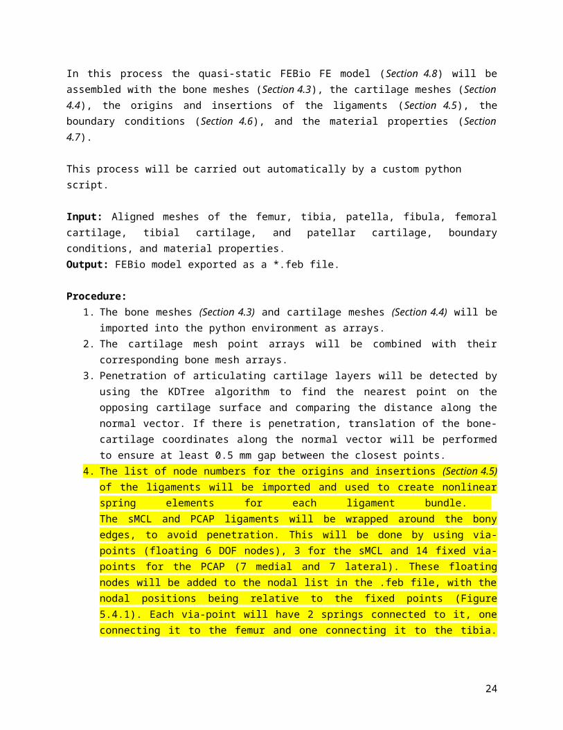
4. The list of node numbers for the origins and insertions (Section 4.5) of the ligaments will be imported and used to create nonlinear spring elements for each ligament bundle. The sMCL and PCAP ligaments will be wrapped around the bony edges, to avoid penetration. This will be done by using via-points (floating 6 DOF nodes), 3 for the sMCL and 14 fixed via-points for the PCAP (7 medial and 7 lateral). These floating nodes will be added to the nodal list in the .feb file, with the nodal positions being relative to the fixed points (Figure 5.4.1). Each via-point will have 2 springs connected to it, one connecting it to the femur and one connecting it to the tibia. The via-points of the sMCL will be connected to the medial fixed point by 3 stiff nonlinear springs.

5. Boundary conditions will be set (Section 4.6).6. The material properties of the bone will be set (Section 4.7.1).7. The material properties of the cartilage will be set (Section 4.7.2).8. Lr of the ligaments will be calculated while the knee is aligned in full extension (0o flexion)

and the material properties (force-displacement curves) of the ligaments and menisci will be initialised (Section 4.7.3).

9. The assembled FE model will be exported as a *.feb file.

17

5.5.1 Global and Anatomical coordinate systemIn this section, the global and anatomical coordinate systems are defined (Figure 5.5.1.1).

Figure 5.5.1.1. Anatomical Coordinate Systems (ACSs) of the patellofemoral (left) and tibiofemoral joint (right) showing anatomical landmarks defined on mesh material points (black points).

The global coordinate system will be defined as the scanner coordinate system. The segmentation point clouds will be obtained in this coordinate system. The FE model will be centered at the origin of this coordinate system.

The anatomical coordinate systems are based on (Grood and Suntay, 1983) using anatomical landmarks (Zhang et al., 2016). The anatomical landmarks are defined on the statistical shape model and embedded as mesh material points (Figure 5.5.1.1).

The ACS for each bone will be used to align the bones to the origin and axes of the global coordinate system during the mesh generation (Section 5.2), where the long axis of the femur will be aligned to the z axis, the medial-lateral axis aligned with the x-axis, and the anterior-posterior axis aligned with the y-axis. The tibia and patella will be aligned relative to the femur and the fibula will be tied to the tibia.

FEBio reports the 6DOF displacements of each rigid body, calculating the relative displacementof its center of mass with respect to its initial position. We will take advantage of this feature of the FEBio software, and set the tibial center of mass to the point between the ACL and PCL tibial attachment zones as described by Grood and Suntay (1983). The center of mass of the patella will be set to be a geometrical mean point of three anatomical landmarks.

18

5.6 Tune ligament properties This section describes how the force-displacement profiles of the ligaments will be optimised given initial ligament material properties (Section 4.7.3).

Input: Assembled FE model of the knee, initial ligament material properties.Output: Tuned ligament material properties, calibrated FE model of the knee.

Procedure:

1. A multi-step objective function will be created in python to take input parameters (stiffness and slack length for each ligament) and give output errors (root-mean-squared differences in bone displacement, flexion-extension angles, varus-valgus angles, and internal-external rotation angles between simulated and expected literature values) for each calibration case (Figure 5.6.1).

2. The objective function will be passed through an optimiser that will attempt to minimise the output errors (i.e. match the displacements and angles) by tuning the input parameters (Figure 5.6.1). The parameters will be considered identical and invariant within ligament bundles and were defined as in Section 4.7.3. Furthermore, the input parameters will be bounded between ± 3 standard deviations of the reported literature values.

Figure 5.6.1. Overview of the multi-step optimisation workflow.

3. The ligament properties will be tuned to passive load-displacement laxity profiles of the tibiofemoral joint at full extension and 90 degrees flexion under anterior-posterior draw of up to 134N and internal-external moment of up to 10 Nm (Li et al., 2002) (Figure 5.6.2).

19

Figure 5.6.2. Passive load displacement laxity profiles of the knee at full extension (0o) and 90o

flexion obtained by (Li et al., 2002) used for ligament tuning.

5.7 Perform simulations and obtaining kinematicsThis section describes how the kinematics of passive knee flexion will be obtained from the calibrated FE model of the knee.

Input: Calibrated FE model of the knee.Output: Kinematic graphs of the tibiofemoral and patellofemoral joints.

Procedure:1. A python script will be used to run FEBio to solve quasi-static FE simulations of passive

knee flexion from 0 to 90 degrees in increments of 10 degrees in FEBio, where passive knee flexion will be applied to the tibia with respect to the femur in the form of a prescribed rotation.

2. Upon completion of each simulation case, the 2 dependent DOF of the tibia (varus-valgus angle and internal-external rotation angle) with respect to the femur will be written to the FEBio log file. The 3 DOF of the patella (medial-lateral tilt, shift, and rotation angles of the patella) with respect to the femur will also be written to the FEBio log file.

3. The log files of each simulation case will be read by the python script and exported to a *.txt file containing the 6 DOF kinematics of the tibiofemoral and patellofemoral joints.

4. The python script will use the 6 DOF kinematics to create six graphs for each degree of freedom of the knee.

20

5.8 Burden The burden will be documented according to the time required of each process (if automatic) or the number of man hours (if manual intervention is required), level of expertise required, and computational cost.

As our processes are mostly automated, the level of expertise will also include in brackets the level of expertise required to automate the process.

Unless otherwise stated, the hardware to be used will be: Intel(R) Core(™) i7-7700HQ CPU @ 2.8GHz, 32.0 GB RAM.

5.8.1 Segmentation Software to be used: Matlab R2017a Academic Licence (+ segmentation scripts)Man hours: Likely to be 1 - 2 days per subject per datasetLevel of expertise: Medium (some anatomical knowledge required to properly segment structures of interest)Computational cost: Low

5.8.2 Bone mesh generation Software to be used: MAP Client (python 2.7 scripts)Time: Likely to be around 25 minutes per subject. Level of expertise: Low (High)Computational cost: Low

5.8.3 Loft cartilageSoftware to be used: Python 2.7Time: Likely to be around 1 minute per subject.Level of expertise: Low (High)Computational cost: Low

5.8.4 Extract ligaments origins and insertionsSoftware to be used: Python 2.7Time: Less than 1 minute per subject.Level of expertise: Low (High)Computational cost: Low

5.8.5 Assembling FE modelSoftware to be used: Python 2.7 Time: Less than 1 minute per subject.Level of expertise: Low (High)Computational cost: Low

21

5.8.6 Tuning ligament material propertiesSoftware to be used: Python 2.7, FEBio version 2.6.4Time: Estimated to be ~24 hrs CPU time per subject. Level of expertise: Low (High)Computational cost: High

22

6. References Baldwin, M. A., Laz, P. J., Stowe, J. Q., & Rullkoetter, P. J. (2009). Efficient probabilistic representation of tibiofemoral soft tissue constraint. Computer methods in biomechanics and biomedical engineering, 12(6), 651-659.

Baldwin, M. A., Langenderfer, J. E., Rullkoetter, P. J., & Laz, P. J. (2010). Development of subject-specific and statistical shape models of the knee using an efficient segmentation and mesh-morphing approach. Computer methods and programs in biomedicine, 97(3), 232-240.

Baldwin, M. A., Clary, C. W., Fitzpatrick, C. K., Deacy, J. S., Maletsky, L. P., & Rullkoetter, P. J. (2012). Dynamic finite element knee simulation for evaluation of knee replacement mechanics. Journal of biomechanics, 45(3), 474-483

Blankevoort, L., Kuiper, J. H., Huiskes, R., & Grootenboer, H. J. (1991). Articular contact in a three-dimensional model of the knee. Journal of biomechanics, 24(11), 1019-1031.

Blankevoort, L., & Huiskes, R. (1996). Validation of a three-dimensional model of the knee. Journal of biomechanics, 29(7), 955-961.

Borbas, P., Koch, P. P., & Fucentese, S. F. (2014). Lateral patellofemoral ligament reconstruction using a free gracilis autograft. Orthopedics, 37(7), e665-e668.

Criscenti, G., De Maria, C., Sebastiani, E., Tei, M. A. T. T. E. O., Placella, G., Speziali, A. N. D. R. E. A., ... & Cerulli, G. (2016). Material and structural tensile properties of the human medial patello-femoral ligament. Journal of the mechanical behavior of biomedical materials, 54, 141-148.

Donahue, T. L. H., Hull, M. L., Rashid, M. M., & Jacobs, C. R. (2002). A finite element model of the human knee joint for the study of tibio-femoral contact. Journal of biomechanical engineering, 124(3), 273-280.

Erdemir, A. (2013). Open knee: a pathway to community driven modeling and simulation in joint biomechanics. Journal of medical devices, 7(4), 040910.

Grood, E. S., & Suntay, W. J. (1983). A joint coordinate system for the clinical description of three-dimensional motions: application to the knee. Journal of biomechanical engineering, 105(2), 136-144.

Guess, T. M., Thiagarajan, G., Kia, M., & Mishra, M. (2010). A subject specific multibody model of the knee with menisci. Medical engineering & physics, 32(5), 505-515.

Harris, M. D., Cyr, A. J., Ali, A. A., Fitzpatrick, C. K., Rullkoetter, P. J., Maletsky, L. P., & Shelburne, K. B. (2016). A combined experimental and computational approach to subject-specific analysis of knee joint laxity. Journal of biomechanical engineering, 138(8), 081004.

23

Kiapour, A., Kiapour, A. M., Kaul, V., Quatman, C. E., Wordeman, S. C., Hewett, T. E., ... & Goel, V. K. (2014). Finite element model of the knee for investigation of injury mechanisms: development and validation. Journal of biomechanical engineering, 136(1), 011002.

LaPrade, R. F., Ly, T. V., Wentorf, F. A., Engebretsen, A. H., Johansen, S., & Engebretsen, L. (2007). The anatomy of the medial part of the knee. JBJS, 89(9), 2000-2010.

LaPrade, R. F., Morgan, P. M., Wentorf, F. A., Johansen, S., & Engebretsen, L. (2007). The anatomy of the posterior aspect of the knee: an anatomic study. JBJS, 89(4), 758-764.

LaPrade, M. D., Kennedy, M. I., Wijdicks, C. A., & LaPrade, R. F. (2015). Anatomy and biomechanics of the medial side of the knee and their surgical implications. Sports medicine and arthroscopy review, 23(2), 63-70.

Lenz, N. M., Mane, A., Maletsky, L. P., & Morton, N. A. (2008). The effects of femoral fixed body coordinate system definition on knee kinematic description. Journal of biomechanical engineering, 130(2), 021014.

Li, G., Gil, J., Kanamori, A., & Woo, S. Y. (1999). A validated three-dimensional computational model of a human knee joint. Journal of biomechanical engineering, 121(6), 657-662.

Li, G., Suggs, J., & Gill, T. (2002). The effect of anterior cruciate ligament injury on knee joint function under a simulated muscle load: a three-dimensional computational simulation. Annals of biomedical engineering, 30(5), 713-720.

Merican, A. M., Sanghavi, S., Iranpour, F., & Amis, A. A. (2009). The structural properties of the lateral retinaculum and capsular complex of the knee. Journal of biomechanics, 42(14), 2323-2329.

Mesfar, W. & Shirazi-Adl A. (2005). Biomechanics of the knee joint in flexion under various quadriceps forces. The Knee, 12(6), 424-34. http://doi.org/10.1016/j.knee.2005.03.004

Mommersteeg, T. J. A., Blankevoort, L., Huiskes, R., Kooloos, J. G. M., Kauer, J. M. G., & Hendriks, J. C. M. (1995). The effect of variable relative insertion orientation of human knee bone-ligament-bone complexes on the tensile stiffness. Journal of biomechanics, 28(6), 745-752.

Morgan, P. M., LaPrade, R. F., Wentorf, F. A., Cook, J. W., & Bianco, A. (2010). The role of the oblique popliteal ligament and other structures in preventing knee hyperextension. The American journal of sports medicine, 38(3), 550-557.

24

Reeves, N. D., Maganaris, C. N., & Narici, M. V. (2003). Effect of strength training on human patella tendon mechanical properties of older individuals. The Journal of physiology, 548(3), 971-981.

Rochcongar, G., Pillet, H., Bergamini, E., Moreau, S., Thoreux, P., Skalli, W., & Rouch, P. (2016). A new method for the evaluation of the end-to-end distance of the knee ligaments and popliteal complex during passive knee flexion. The Knee, 23(3), 420-425.

Steensen, R. N., Dopirak, R. M., & Mcdonald III, W. G. (2004). The Anatomy and Isometry of Themedial Patellofemoral Ligament: Implications for Reconstruction. The American journal of sports medicine, 32(6), 1509-1513.

Upadhyay, N., Vollans, S. R., Seedhom, B. B., & Soames, R. W. (2005). Effect of patellar tendon shortening on tracking of the patella. The American journal of sports medicine, 33(10), 1565-1574.

Yao, J., Salo, A. D., Lee, J., & Lerner, A. L. (2008). Sensitivity of tibio-menisco-femoral joint contact behavior to variations in knee kinematics. Journal of Biomechanics, 41(2), 390-398.

Zaffagnini, S., Colle, F., Lopomo, N., Sharma, B., Bignozzi, S., Dejour, D., & Marcacci, M. (2013). The influence of medial patellofemoral ligament on patellofemoral joint kinematics and patellar stability. Knee Surgery, Sports Traumatology, Arthroscopy, 21(9), 2164-2171.

Zhang, J., Fernandez, J., Hislop-Jambrich, J., & Besier, T. F. (2016). Lower limb estimation from sparse landmarks using an articulated shape model. Journal of biomechanics, 49(16), 3875-3881.

Zielinska, B., & Donahue, T. L. H. (2006). 3D finite element model of meniscectomy: changes in joint contact behavior. Journal of biomechanical engineering, 128(1), 115-123.

25