experimental study and comparative analysis of transformer harmonic behaviour under linear and

Simplified Model for the Non-Linear Behaviour
Representation of Reinforced Concrete Columns
Under Biaxial Bending
H. Rodrigues Civil Engineering Department, University of Aveiro, Portugal
Faculty of Natural Sciences, Engineering and Technology - Oporto Lusophone University
A. Andrade-Campos Department of Mechanical Engineering, University of Aveiro, Portugal
X. Romão, A. Arêde Department of Civil Engineering, Faculty of Engineering, University of Oporto, Portugal
H. Varum, A. Costa Department of Civil Engineering, University of Aveiro, Portugal
SUMMARY:
In the present paper a simplified model is proposed for the force-deformation behaviour of reinforced concrete
members under biaxial loading combined with axial force. The starting point for the model development was an
existing fixed-length plastic hinge element model that accounts for the non-linear hysteretic behaviour at the
element end-sections, characterized by trilinear moment-curvature laws. To take into account the section biaxial behaviour, the existing model was adopted for both orthogonal lateral directions and an interaction function was
introduced to couple the hysteretic response of both directions.
To calibrate the interaction function it were used numerical results, obtained from fibre models, and
experimental results. For the parameters identification, non-linear optimization approaches were adopted,
namely: the gradient based methods followed by the genetic, evolutionary and nature-inspired algorithms.
Finally, the simplified non-linear model proposed is validated through the analytical simulation of biaxial test
results carried out in full-scale reinforced concrete columns.
Keywords: RC columns, non-linear biaxial behaviour, simplified non-linear model, optimization techniques
1. INTRODUCTION
The non-linear models should reproduce the influence of the structural system’s geometry and also of
the distribution of mass and stiffness, in particular the effect of irregularities in terms of stiffness
and/or mass, in plan and in elevation. A vast number of models have been developed to represent the
material’s non-linear behaviour and are typically divided into different categories, namely global models, microscopic models and discrete finite element (member) models (H Rodrigues et al., 2010;
Scott et al., 2008; Taucer et al., 1991).
The importance of study of the tridimensional response of RC buildings is recognized, associated with tridimensional earthquake actions or to building irregularities, which induces a biaxial bending
demand combined with axial load in the columns. Different modelling strategies have been proposed
for the simulation of the biaxial cyclic behaviour of RC elements with axial force. However, it is
recognized that the available biaxial models are not mature enough to be used in practice, nor to be incorporated into codes/standards as has occurred with uniaxial simplified models. Detailed reviews of
the models available can be found in the CEB Report Nº220, “RC Frames under Earthquake Loading –
State of the Art Report” (CEB, 1996), and in Fardis (Fardis, 1991). Besides the theory of fibre models (Petrangeli et al., 1999; Spacone et al., 1992; Taucer et al., 1991), existing analytical models follow
the concepts of classical plasticity (Pecknold, 1974), Mroz’s theory of multi-surface plasticity
(ElMandooh Galal & Ghobarah, 2003; Powell & Chen, 1986; Takizawa et al., 1976), Bouc-Wen (Wen, 1976), hysteresis modelling (Casciati, 1989; Kunnath & Reinhorn, 1990; Romão et al., 2004; C.
H. Wang & Wen, 2000), bounding surface plasticity (Bousias et al., 2002; M.G. Sfakianakis & M.N.
Fardis, 1991; M.G. Sfakianakis & M.N. Fardis, 1991) or lumped damage models (M.E. Marante &
Flórez-López, 2002; Maria Eugenia Marante & Flórez-López, 2003; Mazza & Mazza, 2008).
The present paper proposes an upgraded simplified model for the representation of the biaxial bending
response of columns with axial force, which is based in an existing uniaxial hysteretic Costa-Costa
model (Costa & Costa, 1987). The general formulation of the proposed model is established in the analogy and comparison with the
biaxial formulation of the Bouc-Wen smooth hysteretic model [9]. Although retaining most of the
physical meaning embodied in the Bouc-Wen model, the structural modelling strategy adopted retains the simplicity and versatility of the original piecewise linear (PWL) numerical tool.
2. COSTA AND COSTA UNIAXIAL HYSTERETIC MODEL
For the development and validation of the simplified biaxial model, the Costa-Costa uniaxial
hysteretic model (CEB, 1996; Costa & Costa, 1987) was adopted, which is briefly described in the next paragraph.
This model represents a generalisation of the original Takeda model (CEB, 1996; Takeda et al., 1970)
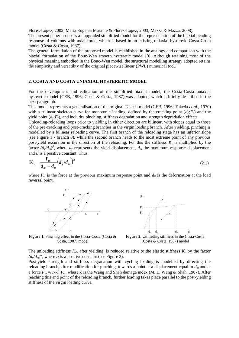
with a trilinear skeleton curve for monotonic loading, defined by the cracking point (dc;Fc) and the yield point (dy;Fy), and includes pinching, stiffness degradation and strength degradation effects.
Unloading-reloading loops prior to yielding in either direction are bilinear, with slopes equal to those
of the pre-cracking and post-cracking branches in the virgin loading branch. After yielding, pinching is modelled by a bilinear reloading curve. The first branch of the reloading stage has an inferior slope
(see Figure 1 - branch 8), while the second branch heads to the most extreme point of any previous
post-yield excursion in the direction of the reloading. For this the stiffness Ks is multiplied by the
factor (dy/dm), where dy represents the yield displacement, dm the maximum response displacement
and is a positive constant. Thus:
my
0
m
s /F
K ddddm
(2.1)
where Fm is the force at the previous maximum response point and d0 is the deformation at the load reversal point.
Figure 1. Pinching effect in the Costa-Costa (Costa &
Costa, 1987) model
Figure 2. Unloading stiffness in the Costa-Costa
(Costa & Costa, 1987) model
The unloading stiffness Kd, after yielding, is reduced relative to the elastic stiffness Ke by the factor
(dy/dm), where is a positive constant (see Figure 2).
Post-yield strength and stiffness degradation with cycling loading is modelled by directing the
reloading branch, after modification for pinching, towards a point at a displacement equal to dm and at
a force F’m=(1-)·Fm, where is the Wang and Shah damage index (M. L. Wang & Shah, 1987). After
reaching this end point of the reloading branch, further loading takes place parallel to the post-yielding
stiffness of the virgin loading curve.
6
F-
m
md -
12
13
7
5
8
K
1
2
9
F
4
d m+
d
3
11
10
mF+
s
dd c y
F c
F y
F
d m d
Kd
eK

3. THE BIAXIAL BOUC-WEN MODEL
The original formulation of the Bouc-Wen model, cast within the endochronic theory framework was
presented by Bouc (Bouc, 1971), for uniaxial behaviour representation (in terms of Force-Displacement, F-u), and it was later generalized by Wen (Wen, 1976). The generalized model
expresses the restoring force as a combination of an elastic force and a plastic force: Z
yFuK )1(F (3.1)
where K is the initial stiffness, the post-yielding stiffness ratio, Fy the yielding force, and Z is a hysteretic parameter.
Later, this uniaxial formulation was extended by Park, Wen and Ang (Park et al., 1986; Wen, 1976) to define a biaxial force-deformation model with coupled differential equations. This model was then
used and modified by Kunnath and Reinhorn (Kunnath & Reinhorn, 1990) to model the behaviour of
RC columns under biaxial loads. Later on, the model was generalised by Casciati (Casciati, 1989) and also by Wang and Wen (C. H. Wang & Wen, 2000), which resulted in two different formulations of
the initial biaxial model. Since the Wang and Wen (C. H. Wang & Wen, 2000) formulation is simpler,
it was selected for to implementing the biaxial model proposed in this work. Nevertheless, the same mathematical reasoning can be applied to the Casciati (Casciati, 1989) form.
The biaxial construction of the Bouc-Wen model in the Wang and Wen (C. H. Wang & Wen, 2000)
form follows the same general idea as for the uniaxial case. The restoring forces for both directions are defined by:
(3.2)
in which the involved parameters have the same meaning as for the uniaxial case, but are now referred
to the two orthogonal directions X and Y, by the subscripts x and y respectively. The hysteretic parameters Zx and Zy are then defined by the following coupled differential equations, where all the
parameters involved have also the same meaning as for the uniaxial case and sign() refers to the
mathematical signum function.
(3.3)
As for the case of the uniaxial model, Equation 3.2 can also be reformulated into an incremental form:
(3.4)
considering that the global restoring forces ixF and
iyF result from:
(3.5)
Considering now the definition of the incremental orthogonal forces ixF and
iyF given by, the first
part of this system can be written, by a simple mathematical transformation, as:
(3.6)
yy
yyyyyy
xy
xxxxxx
ZF1uKF
ZF1uKF
yy
xx
1n
xyxyy
1n
yyyy
y
yx
yy
1n
yxyxx
1n
xxxx
x
u
ZusignZZuZusignZZuuAZ
u
ZusignZZuZusignZZuuAZ
yy
yyyyyy
xy
xxxxxx
ZF1uKF
ZF1uKF
i1ii
i1ii
yyy
xxx
FFF
FFF
iiiiiiii
iiiiiiii
yy
1n
yyyyyyyyyy
xx
1n
xxxxxxxxxx
ZusignZZuuAK1uKF
ZusignZZuuAK1uKF

which matches to the uniaxial incremental restoring forces calculated for each direction without
biaxial interaction. In order to simplify the notation, these incremental forces will be denoted as
ixuniF and
iyuniF , respectively. The remaining part of the system corresponds to the correction
factors ifxC and
ifyC accounting for the interaction between the two loading directions:
(3.7)
Therefore, based on Equations 3.6 and 3.7, a condensed form of Equation 4 can be written as:
fyiC
iyuni
Fi
yF
fxiC
ixuni
Fi
xF
(3.8)
Considering that the incremental forces ixuniF
and iyuniF
can be obtained with any uniaxial hysteretic
model (particularly with well-established PWL models), the presented framework introduces a simple and flexible form to represent biaxial bending in columns. This formulation requires the same
information needed for the corresponding uniaxial PWL model, only introducing an additional
correction term which couples the two loading directions.
Since the uniaxial hysteretic model that may be considered to obtain the incremental forces ixuniF
and
iyuniF could be very different from the original uniaxial Bouc-Wen formulation, the type and level of
biaxial interaction between the two orthogonal directions can be also different. Romão et al. (Romão
et al., 2004) proposed an additional parameter , which was included in Equation 3.8 in order to scale the level of interaction between the two loading directions. The final formulation of the proposed method is then defined as written in Equation 3.9, which states that for each incremental
displacements vector iyix uu ; , the incremental forces
ixuniF and
iyuniF can be separately calculated,
as:
(3.9)
The values of the scaling interaction factor will be defined as for the best-fitting of the numerical
results to the experimental results obtained with biaxial tests, additional information about the presented formulation can be found in the literature (Romão et al., 2004).
4. PARAMETER IDENTIFICATION FOR THE SCALING INTERACTION FACTOR
4.1 Optimization method
Numerical non-linear simplified models may play an important role in the design of new structures
and in the assessment of existing ones. More complex techniques and models have been developed to
simulate, with increasing accuracy, the behaviour of different materials and structures. However, many of these simulation models require the determination and calibration of a large number of parameters
adjusted to the specific material and structural problem.
The identification of parameters for the mathematical models adopted to describe the behaviour of physical systems is a common problem in engineering. The complexity of the models, as well as the
number of parameters associated, normally increases with the complexity of the physical system. The
determination of these parameters should be based on the comparison of the mathematical model
results and experimental results. However, when the required number of experimental tests and
iiiiii
iiiiii
xx
1n
xyxyyfy
yy
1n
yxyxxfx
ZusignZZuK1C
ZusignZZuK1C
iii
iii
fyyuniy
fxxunix
CFF
CFF

parameters increases, it may become impractical to identify the accurate parameters (Andrade-Campos
et al., 2007; Bruhns & Anding, 1999). In these cases, it may be used an inverse formulation for the
identification of parameters. This approach often leads to the resolution of a non-linear optimization
problem. In this work, aiming at calibrating the parameters for the hysteretic biaxial model based on uniaxial
models with an interaction function, a gradient based-method (Levenberg-Marquardt (LM) method)
was adopted, sequentially associated with an evolutionary algorithm method (real search space EA), grouped. With these global cascade algorithms, it is intended to aggregate the advantages of both
algorithms and to minimise their disadvantages (Andrade-Campos et al., 2009).
For the application of these models, the SDL/SiDoLo optimisation lab computer program was used (Andrade-Campos, 2011). The program was designed for specific engineering inverse problems, such
as parameter identification and initial shape optimization problems. It inherits the wealth of experience
gained in such problems by the previous SIDOLO code, and adds the latest developments in direct
search optimization algorithms (Andrade-Campos, 2011; Andrade-Campos et al., 2007).
4.2 Prediction and optimization of the scaling factor equation
The calibration of the interaction function, using the optimization strategies presented in the previous
section, was performed in two phases. In the first phase, it was intended to select the analytical
expression-type most suitable for the interaction scaling factor () function. After the expression type selection, the second phase, consists in the calibration of the parameters of the interaction function as
well as of the interaction scaling factor. The parameters’ calibration corresponds to the best-fit of the results for a group of numerical analyses.
In order to define the interaction scaling factor () which characterizes the level of interaction, as a function dependent of the section properties and loading direction, a set of numerical analyses was
performed. To this aim, twenty seven rectangular RC columns were defined, varying in cross-section
dimensions (30x30, 30x50 and 30x60), reinforcing steel ratio (1%, 1.5% and 2%) and axial load ratio (0.1, 0.2 and 0.3). For the column, a cantilever 1.5m high was considered. The response of each
column was obtained with pushover analysis for different directions Columns were modelled with a
force-based element formulation and considering a fibre discretization at the section level. Two uniaxial (0º and 90º) and five biaxial (at 11.25º, 22.5 º, 45 º, 67.5 º, 78.75 º angles) pushover analyses
were performed using the computer program SeismoStruct (SeismoSoft, 2004).
An interaction scaling factor was determined for each biaxial response of each column, based on the
Costa-Costa uniaxial model coupled with the proposed interaction function previously presented in Equation 3.9. For these analyses, a gradient-based optimization algorithm was used (Andrade-Campos
et al., 2007). In order to reduce the number of variables, for the shape factors (γ, and n) necessary to
calculate ifxC and
ifyC were assumed equal to the values suggested by Kunnath and Reinhorn were
adopted ( 5.0 and 2n ).
Aiming at evaluating the goodness-of-fit of the given interaction scaling factor, for each column and
for each direction calculation are made for, the difference between the simulated response with the simplified (sim) model (with the interaction function parameters) and with the refined numerical
model (reference values, ref). These differences are evaluated for each direction (X or Y) by the
Relative Global Error (RGEdirection), as given in Equation 4.1. The combination of the error for the
two directions (RGEtotal) is calculated as presented in Equation 4.2.
[ ] ∑(
)
(4.1)
√
(4.2)
where and
are, respectively, the simulated and reference values of the potential energy
associated with each pushover response.

After obtained the optimal values of the scaling factor () for each analysis (each column and each
direction), an expression type was selected (see Equation 4.3), which depends on the column properties, namely the cross-section dimensions (h and b), the axial load ratio (ν); and loading
direction (α).
(
)
( ) (4.3)
The four constants (C1, C2, C3, and C4) are to be obtained by optimization for all pushover curves, as
will be shown in the following Section.
With the adopted equation for the scaling factor, the interaction function parameters were optimized for all biaxial pushover curves, using a cascade optimization strategy.
At this stage, the Levenberg-Marquardt (LM) gradient-based method and an evolutionary method (real
search space EA) were grouped in sequential/cascade strategies. Thus, as mentioned before, in order to combine the advantages of both algorithms and minimise their disadvantages, the following sequence
LM+EA+LM was used.
An important aspect in a cascade algorithm is the choice of the criteria to switch from one optimizer to another. In the present case, a heuristic approach was adopted based on numerical experiments. The
criteria, as suggested in (Andrade-Campos et al., 2009), were: i) Switching from LM to EA: if, from
one iteration to another, the relative decrease in the quadratic objective function is less than 1×10-15, or the maximum admissible iteration number (predetermined value) is reached. ii) Switching from EA
to LM: if stagnation of more than 500 generations is observed or the relative decrease in the quadratic
objective function is less than 1×10-15 or the maximum admissible iteration number (predetermined value) is reached. The obtained results are summarized in Table 1 and the convergence evolution of
the cascade optimization strategies in the parameter identification are presented in Figure 3. Table 1. Parameters achieved by the cascade
optimization strategy
Parameter Value
0.37
0.90
n 2.00
C1 1.00
C2 0.23
C3 0.45
C4 -0.52
Figure 3. Convergence evolution of the cascade optimization
strategies in the parameter identification
Figure 4 shows the plot of the Relative Global Error, calculated for each direction (using Equation 4.1), for two situations, in order to compare the reference simulation with the simplified model results,
with and without considering the interaction function, represented in the figure with filled and unfilled
marks respectively). By comparing the Relative Global Errors for the two situations the error reduction in each direction is clear when the interaction function is considered.
Figure 5 includes a selected group of examples of pushover curves for different columns and different
pushover loading angles. In each plot, for both directions, the obtained pushover curves are represented: i) by the refined numerical fibre model (reference curves – blue lines with square marks);
ii) by the simplified model without the biaxial bending interaction function (red lines with trianglular
marks); and iii) by the simplified model but with the interaction function (the optimised solution – green lines with diamond marks). Also, the examples in Figure 5 confirm the error reductions, in both
column directions, obtained by adopting the interaction function combined with the optimized scaling
factor.
0 500 1000 1500 2000
1.0x10⁷
1.2x10⁷
1.4x10⁷
1.6x10⁷
1.8x10⁷
2.0x10⁷
2.2x10⁷
2.4x10⁷
2.6x10⁷
Qua
drat
ic e
rror
Iterations/Generations
LM+EA+LM
0 20 40 60 80 100 120 140 160 180 200
1.0x10⁷
1.2x10⁷
1.4x10⁷
1.6x10⁷
1.8x10⁷
2.0x10⁷
2.2x10⁷
2.4x10⁷
2.6x10⁷
LM

Figure 4. Relative Global Error (X and Y column directions) of the simplified model results, with (filled marks)
and without (unfilled marks) interaction function, compared with the refined numerical model results
Figure 5. Examples of pushover curves for different columns and different pushover loading angles for the refined numerical model, the simplified model without the biaxial bending interaction function and the
simplified model with the interaction function
5. VALIDATION OF THE MODEL WITH RESULTS FROM CYCLIC TESTS
5.1 Introduction
For the validation of the proposed simplified model with interaction functions, the experimental results
of cyclic tests on 8 RC columns were used of the test campaign (H. Rodrigues et al., 2012; H.
Rodrigues, 2012). First, the uniaxial tests were modelled in order to obtain the primary skeleton curves for each independent direction. Then, using the obtained curves, the biaxial tests were simulated and
the results of the numerical model with the interaction function are compared with the test results.
5.2 Analysis of the results
For the validation of the proposed simplified interaction model, a trilinear envelope curve was
considered for the primary curve of each column direction, by best-fit adjustment to the uniaxial experimental results.
For all uniaxially tested columns, the experimental results were well reproduced with the adjusted
0 50 100 150 200 250
0
50
100
150
200
250
300
350
400
450
500
With interaction function optimized - 11.25º
With interaction function optimized - 22.50º
With interaction function optimized - 45.00º
With interaction function optimized - 67.50º
With interaction function optimized - 78.75º
Without interaction function - 11.25º
Without interaction function - 22.50º
Without interaction function - 45.00º
Without interaction function - 67.50º
Without interaction function - 78.75º
Rel
ativ
e G
loba
l Err
or in
dire
ctio
n Y
(%
)
Relative Global Error in direction X (%)
0.00 0.01 0.02 0.03 0.04 0.050
50
100
150
200
250
300
350
400
450
500
550
M26
30x60cm2
= 0.2
As = 2.0% Ac
Pushover - 11.25o
Bas
e Sh
ear
(kN
)
Horizontal Displacement (m)
Fibre model (X direction)
Fibre model (Y direction)
Original (X)
Original (Y)
Optimized solution (X)
Optimized solution (Y)
0.00 0.01 0.02 0.03 0.04 0.050
50
100
150
200
250
300
350
Bas
e Sh
ear
(kN
)
Horizontal Displacement (m)
Fibre model (X direction)
Fibre model (Y direction)
Original (X)
Original (Y)
Optimized solution (X)
Optimized solution (Y)
M16
30x50cm2
= 0.1
As = 1% Ac
Pushover - 22.5o
0.00 0.01 0.02 0.03 0.04 0.050
50
100
150
200
250
300
350
400
M22
30x60cm2
= 0.1
As = 1.5% Ac
Pushover - 45o
Bas
e Sh
ear
(kN
)
Horizontal Displacement (m)
Fibre model (X direction)
Fibre model (Y direction)
Original (X)
Original (Y)
Optimized solution (X)
Optimized solution (Y)
0.00 0.01 0.02 0.03 0.040
50
100
150
200
250
300
350
M14
30x50cm2
= 0.2
As = 1.5% Ac
Pushover - 45o
Bas
e Sh
ear
(kN
)
Horizontal Displacement (m)
Fibre model (X direction)
Fibre model (Y direction)
Original (X)
Original (Y)
Optimized solution (X)
Optimized solution (Y)

uniaxial trilinear curves and with the hysteretic rules of the original model, as represented in Figure 6.
In the figures the following are plotted for each column: the numerical calculations with the
interaction model (blue); the experimental results (red); and the trilinear primary curve (green).
As observed in these figures, the strength degradation is difficult to represent, particularly for the last
cycles of the experimental response. However, significant differences are only observed for demands
corresponding to drifts greater than 2.5%. The energy dissipation evolution is also well represented. Again, only for the last cycles (associated with the differences in terms of strength degradation), an
overestimation of the dissipated energy is obtained with the numerical model.
In order to validate the rules and parameters of the interaction model for the simulation of the biaxial
response of the tested RC columns, the trilinear curve adjusted to the uniaxial test results was
considered for the primary curve in each direction.
The prediction of the experimental biaxial response obtained with the simplified interaction model for
the tested RC columns is represented in Figures 7, 8 and 9. The same line legend is adopted as for the
uniaxial cases.
As can be observed, the maximum strength was properly obtained with the simplified biaxial model.
For the columns strong directions, a underestimation of the maximum strength of 15% was observed, while overestimation of 25% is reached in the weak direction. The unloading stiffness and the
pinching effect were reasonably reproduced in most cases.
The strength degradation was also reasonably approximately in the examples under analysis. Only in
the latter stages of the columns’ response, close to the columns’ failure, considerable differences were detected in terms of strength degradation.
The evolution of the accumulated energy dissipation is reasonable well simulated until noticeable strength degradation is observed. In the stronger column direction an overestimation of around 20%
was reached and in the weak direction the underestimation is around 25%.
In general, a good agreement between the predicted numerical results and the experimental hysteretic response was observed, indicating that the proposed strategy may be suitable to simulate the response
of columns to biaxial loading based on uniaxial behaviour curves associated with properly calibrated
coupling interaction functions.
Figure 6 – Base-shear versus drift of column N13 – Uniaxial test
Figure 7. Base-shear versus drift of column N14 – Biaxial test, rhombus displacement pattern

Figure 8. Base-shear versus drift of column N15 – Biaxial test, quadrangular displacement pattern
Figure 9. Base-shear versus drift of column N16 – Biaxial test, circular displacement pattern
6. CONCLUSIONS AND FINAL COMMENTS
There are still a number of unsolved problems associated with modelling of RC elements under biaxial loading. Simplified biaxial models may be adopted if they can adequately reproduce the main
characteristics of the element’s response (such as the strength and stiffness degradation, ductility, and
energy dissipation capacity) relative to the columns uniaxial response.
In the present paper, a simplified interaction model for the response of RC columns to biaxial loading
is described, based on existing uniaxial models. The proposed model corresponds to an upgrade of the existing Costa-Costa uniaxial hysteretic model, and adopts an interaction function based on the Bouc-
Wen biaxial hysteretic model, coupling the two loading directions. The model parameters were
calibrated using optimization techniques, based on the results of a parametric study on the
tridimensional response of RC columns models with a refined model. The validity of the proposed model was demonstrated through the analytical simulation of biaxial tests on RC columns. The
obtained numerical results were adequate and proved the efficiency of the model, which is a simple
tool capable of reproducing the response of RC elements considering the biaxial interaction.
The proposed simplified model can be a useful tool in the design and assessment of RC structures
where the response is dependent on biaxial bending of the elements. This non-linear model accounts
for mechanical features such as hysteretic behaviour rules, strength and stiffness degradation, and the pinching effect. However, additional research is still necessary to objectively define the interaction
function parameters, which establish the coupling of the response in the two loading directions.
Moreover, the model application to experimental results obtained by other authors should be made. The implementation of the proposed model in a structural analysis program to obtain the response of
RC multi-storey buildings (which strongly depends on the biaxial response of the columns) is another
important task that should be archived.
-4 -2 0 2 4-100
-75
-50
-25
0
25
50
75
100
0
20
40
60
80
100
120
-4 -2 0 2 4-100
-75
-50
-25
0
25
50
75
100
0
20
40
60
80
Drift Y (%)
Drift X (%)
Step
Acc
umul
ativ
e hy
ster
esis
diss
ipat
ed e
nerg
y (k
N.m
)
Step
Acc
umul
ativ
e hy
ster
esis
diss
ipat
ed e
nerg
y (k
N.m
)
Shea
r Y
(kN
)Sh
ear
X (
kN)
PB12-N16
X
Y
X
PB12-N16
X
Y
X

REFERENCES Andrade-Campos, A. (2011). Development of an Optimization Framework for Parameter Identification and Shape
Optimization Problems in Engineering. International Journal of Manufacturing, Materials, and Mechanical
Engineering (IJMMME), 1(1), 57-79. doi: doi:10.4018/ijmmme.2011010105 Andrade-Campos, A., Pilvin, P., Simões, J., & Teixeira-Dias, F. (2009). Software Development for Inverse Determination of
Constitutive Model Parameters Software Engineering: New Research: Nova Science Publishers, Inc. Andrade-Campos, A., Thuillier, S., Pilvin, P., & Teixeira-Dias, F. (2007). On the determination of material parameters for
internal variable thermoelastic–viscoplastic constitutive models. International Journal of Plasticity, 23(8), 1349-1379. doi: 10.1016/j.ijplas.2006.09.002
Bouc, R. (1971). Modèle mathématique d’hystérésis. , Acustica, 24, 16-25. Bousias, S. N., Panagiotakos, T. B., & Fardis, M. N. (2002). Modelling of RC members under cyclic biaxial flexure and axial
force. Journal of Earthquake Engineering, 6, No 2, 213-238. Bruhns, O. T., & Anding, D. K. (1999). On the simultaneous estimation of model parameters used in constitutive laws for
inelastic material behaviour. International Journal of Plasticity, 15(12), 1311-1340. doi: 10.1016/s0749-6419(99)00046-7 Casciati, F. (1989). Stochastic dynamics of hysteretic media. Structural Safety, V. 6(2-4), 259-269. CEB. (1996). RC frames under earthquake loading. Lausanne. Costa, A. C., & Costa, A. G. (1987). Hysteretic model of force-displacement relationships for seismic analysis of structures.
Lisbon, : National Laboratory for Civil Engineering. ElMandooh Galal, K., & Ghobarah, A. (2003). Flexural and shear hysteretic behaviour of reinforced concrete columns with
variable axial load. Engineering Structures, 25(11), 1353-1367. doi: Doi: 10.1016/s0141-0296(03)00111-1 Fardis, M. N. (1991). Member-type models for the nonlinear seismic response of reinforced concrete structures. In D. a. P.
M. Jones (Ed.), Experimental and Numerical Methods in Earthquake Engineering: Kluwer Academic Publishers, Dordrecht, The Netherlands.
H. Rodrigues, A. Arêde, H. Varum, & A.G. Costa. (2012). Experimental evaluation of rectangular reinforced Concrete column behaviour under biaxial cyclic Loading. Earthquake Engineering and Structural Dynamics (in press).
Kunnath, S. K., & Reinhorn, A. M. (1990). Model for inelastic biaxial bending interaction of RC beam-columns. ACI Structural Journal, 87 (3), 284-291.
Marante, M. E., & Flórez-López, J. (2002). Model of damage for RC elements subjected to biaxial bending. Engineering
Structures, 24(9), 1141-1152. doi: doi:10.1016/S0141-0296(02)00044-5 Marante, M. E., & Flórez-López, J. (2003). Three-dimensional analysis of reinforced concrete frames based on lumped
damage mechanics. International Journal of Solids and Structures, 40(19), 5109-5123. doi: Doi: 10.1016/s0020-7683(03)00258-0
Mazza, F., & Mazza, M. (2008). A numerical model for the nonlinear seismic analysis of three-dimensional RC frames. Paper presented at the The 14th World Conference on Earthquake Engineering, Beijing, China.
Park, Y. J., Wen, Y. K., & Ang, A. H.-S. (1986). Random vibration of hysteretic systems under bi-directional ground motions. Earthquake Engineering and Structural Dynamics, 14, 543-557.
Pecknold, D. (1974). Inelastic structural response to 2D ground motion. ASCE J. Eng. Mech. Div., 100(5), 949-963. Petrangeli, M., Pinto, P. E., & Ciampi, V. (1999). Fiber element for cyclic bending and shear of RC structures. I: Theory.
Journal of Engineering Mechanics, 125(9), 994-1001. doi: 10.1061/(asce)0733-9399(1999)125:9(994) Powell, G. H., & Chen, P. F. (1986). 3D beam-column element with generalized plastic hinges. ASCE J. Eng. Mech. Div., V.
112(7), 627-641. Rodrigues, H. (2012). Biaxial seismic be ehaviour of reinforced concrete columnns. PhD Thesis, University of Aveiro, Aveiro. Rodrigues, H., Varum, H., & Costa, A. (2010). Simplified macro-model for infill masonry panels. Journal of Earthquake
Engineering, 14(3), 390-416. doi: 10.1080/13632460903086044
Romão, X., Costa, A., & Delgado, R. (2004). New model for the inelastic biaxial bending of reinforced concrete columns. Paper presented at the 13th World Conference on Earthquake Engineering, Vancouver, B.C., Canada.
Scott, M. H., Fenves, G. L., McKenna, F., & Filippou, F. C. (2008). Software patterns for nonlinear beam-column models. Journal of Structural Engineering, 134(4), 562-571.
SeismoSoft. (2004). SeismoStruc- A computer program for static and dynamic nonlinear analysis of framed structures [online]: Available from URL: http://www.seismosoft.com.
Sfakianakis, M. G., & Fardis, M. N. (1991). Bounding surface model for cyclic biaxial bending of RC sections. Journal of Engineering Mechanics, 117(12), 2748-2769. doi: 10.1061/(ASCE)0733-9399(1991)117:12(2748)
Sfakianakis, M. G., & Fardis, M. N. (1991). RC Column model for inelastic seismic response analysis in 3D. Journal of Engineering Mechanics, 117(12 ), 2770-2787. doi: 10.1061/(ASCE)0733-9399(1991)117:12(2770)
Spacone, E., Ciampi, V., & Filippou, F. (1992) A beam element for seismic damage analysis. Vol. UCB/EERC-92/07. University of California, Berkeley: Earthquake Engineering Research Center.
Takeda, T., Sozen, M. A., & Nielsen, N. N. (1970). Reinforced Concrete Response to Simulated Earthquakes. ASCE, Journal of the Structural Division, 96(ST12).
Takizawa, H., Aoyama, M., & . (1976). Biaxial effects in modelling earthquake response of RC structures. Earthq. Engrg and Struct. Dynamics, V. 4, 523-552.
Taucer, F., Spacone, E., & Filippou, F. (1991). A fiber beam-column element for seismic response analysis of reinforce
concrete structures: University of California, Berkeley. Wang, C. H., & Wen, Y. K. (2000). Evaluation of pre-Northridge low-rise steel buildings. I: Modelling J. Struct. Eng.,
ASCE, V. 126(10), 1160-1168. Wang, M. L., & Shah, S. P. (1987). Reinforced concrete hysteresis model based on the damage concept. Earthquake
Engineering & Structural Dynamics, 15(8), 993-1003. doi: 10.1002/eqe.4290150806 Wen, Y. K. (1976). Method for random vibration of hysteretic systems. ASCE J. Eng. Mech. Div., 102(EM2), 249-263.