SIMPLIFIED BOW MODEL - vtechworks.lib.vt.edu · with conventional FE model results, closed-form...
251
SIMPLIFIED BOW MODEL FOR A STRIKING SHIP IN COLLISION by Suryanarayana Vakkalanka Thesis submitted to the faculty of the Virginia Polytechnic Institute and State University In partial fulfillment of the requirements for the degree of MASTER OF SCIENCE in Ocean Engineering APPROVED: A.J. Brown, Chairman R.K Kapania O. Hughes March 2000 Virginia Tech, Blacksburg, VA, USA Keywords: ship, collision, bow, damage, accident Copyright © 2000, Suryanarayana Vakkalanka
Transcript of SIMPLIFIED BOW MODEL - vtechworks.lib.vt.edu · with conventional FE model results, closed-form...
SIMPLIFIED BOW MODEL FOR A STRIKING SHIP IN COLLISION
by Suryanarayana Vakkalanka
Thesis submitted to the faculty of the Virginia Polytechnic Institute and State University
In partial fulfillment of the requirements for the degree of
MASTER OF SCIENCE in
Ocean Engineering
APPROVED:
A.J. Brown, Chairman
R.K Kapania O. Hughes
March 2000 Virginia Tech, Blacksburg, VA, USA
Keywords: ship, collision, bow, damage, accident Copyright © 2000, Suryanarayana Vakkalanka
ABSTRACT
SIMPLIFIED BOW MODEL
FOR A STRIKING SHIP IN COLLISION
by Suryanarayana Vakkalanka
The serious consequences of ship collisions necessitate the development of
regulations and requirements for the subdivision and structural design of ships to reduce
damage and environmental pollution, and improve safety.
Differences in striking ship bow stiffness, draft, bow height and shape have an
important influence on the allocation of absorbed energy between striking and struck
ships. The energy absorbed by the striking ship may be significant. The assumption of a
“rigid” striking bow may no longer hold good and typical simplifying assumptions may
not be sufficient.
The bow collision process is simulated by developing a striking ship bow model
that uses Pedersen's super-element approach and the explicit non-linear FE code LS-
DYNA. This model is applied to a series of collision scenarios. Results are compared
with conventional FE model results, closed-form calculations, DAMAGE, DTU,
ALPS/SCOL and SIMCOL. The results demonstrate that the universal assumption of a
rigid striking ship bow is not valid. Bow deformation should be included in future
versions of SIMCOL.
A simplified bow model is proposed which approximates the results predicted by
the three collision models (closed-form, conventional and intersection elements) to a
reasonable degree of accuracy. This simplified bow model can be used in further
calculations and damage predictions. A single stiffness can be defined for all striking
ships in collision, irrespective of size.
ACKNOWLEDGEMENTS
The completion of this thesis would have been impossible without the support of
many people. First of all, I would like to express my sincere appreciation to my advisor,
Professor Alan Brown, for his continuous support and guidance throughout the duration
of this work. He has been a constant source of inspiration and it has been a pleasure
working under his supervision.
This thesis is dedicated to my parents, Sri V.N Pratap & Smt. V. Ramavathi and
my sister, Sita who have been a constant source of encouragement. Their love and
support have helped me through difficult times and keep up challenges.
Also, I would like to acknowledge the support of several research students
working on the ship collision project, particularly Donghui Chen, Bo Jin, Marie Lutzen
and Jianjun Xia for helpful discussions.
I am grateful to the Department of Aerospace & Ocean Engineering at Virginia
Tech. for providing me with research assistantship throughout the course of my study. I
would like to thank ETA (Engineering Technology Associates), MI and LSTC
(Livermore Software Technology Corporation), CA for providing technical support when
needed and for providing introductory training in LS-DYNA. I am also thankful to the
Society of Naval Architects and Marine Engineers (SNAME) and Ship Structure
Committee (SSC) for funding this project.
I am thankful to Dr. Rakesh Kapania and Dr. Owen Hughes for serving on the
committee and for their valuable suggestions. Finally, I would like to thank “our gang”,
especially Susmitha Akula, who made my stay in Blacksburg and in the U.S.A a very
pleasant and memorable one.
TABLE OF CONTENTS
ABSTRACT
ACKNOWLEDGEMENTS
LIST OF TABLES i
LIST OF FIGURES ii
CHAPTER 1 INTRODUCTION 1
1.1 MOTIVATION [1, 2, 3, 4]................................................................................................................................ 1
1.1.1 Revision of IMO Regulations 1
1.1.2 SNAME/SSC Collision and Grounding Research Project 2
1.1.3 Collision Model for Probabilistic Analysis 3
1.2 HYPOTHESIS..................................................................................................................................................... 5
1.3 PLAN................................................................................................................................................................. 6
1.4 THESIS ORGANIZATION.................................................................................................................................. 7
CHAPTER 2 COLLISION SCENARIOS AND DATA 8
2.1 COLLISION SCENARIO VARIABLES............................................................................................................... 8
2.2 RIGID BOW GEOMETRY............................................................................................................................... 14
2.3 SIMCOL BOW MODEL................................................................................................................................ 17
CHAPTER 3 BOW DAMAGE MODELS 19
3.1 INTRODUCTION ....................................................................................................................................... 19
3.2 MINORSKY [40] ............................................................................................................................................. 19
3.3 RIGID BOW MODELS.................................................................................................................................... 22
3.3.1 Hutchison [25] 22
3.3.2 Ito [27] 25
3.3.3 Wierzbicki [68] 27
3.3.4 MIT “DAMAGE” – Simonsen [62] 28
3.3.5 SIMCOL [17] 31
3.4 DEFORMABLE BOW MODELS...................................................................................................................... 32
3.4.1 Woisin [69] 32
3.4.2 Kim [30] 34
3.4.3 Gerard [52] 36
3.4.4 Amdahl [5, 6] 37
3.4.5 Yang and Caldwell [70] 38
3.4.6 Kierkegaard [29] 43
3.4.7 Valsgard and Pettersen [66] 46
3.4.8 Pedersen [52] 49
3.5 COMPARISON OF THE MODELS.................................................................................................................... 56
CHAPTER 4 EVIDENCE SUPPORTING THE HYPOTHESIS 57
4.1 INTRODUCTION ....................................................................................................................................... 57
4.2 PICTORIAL EVIDENCE .......................................................................................................................... 57
4.3 RECKLING ANALYSIS OF ABSORBED ENERGY [58]................................................................ 59
4.4 EXPERIMENTAL RESULTS [31, 66] .................................................................................................. 63
4.5 MINORSKY CALCULATIONS.............................................................................................................. 64
CHAPTER 5 AN OVERVIEW OF FEMB,LS-DYNA3D AND POSTGL 67
5.1 INTRODUCTION.............................................................................................................................................. 67
5.2 FEATURES OF THE PRE-PROCESSOR, FEMB 26 NT ............................................................................... 67
5.2.1 Mesh Generation 68
5.2.2 Material Properties 68
5.2.3 Contact Interface 69
5.2.4 Specifications/database limitations 70
5.2.5 Line data 70
5.2.6 Recommended Practice (.fmb, .his, .lin, .bin, etc.) 70
5.2.7 Local coordinate system 71
5.2.8 Getting started with FEMB 72
5.2.9 Getting started with CAD data 72
5.2.10 Main menu 73
5.3 LS-DYNA VERSION 950.......................................................................................................................... 82
5.3.1 Sense switch controls 83
5.3.2 LS-DYNA contact algorithm 84
5.4 POST PROCESSOR, ETA POSTGL.................................................................................................................. 86
5.4.1 PostGL/Graph 87
CHAPTER 6 BOW AND HULL MODELS DEVELOPED IN LSDYNA 89
6.1 INTRODUCTION.............................................................................................................................................. 89
6.2 TEST CASE MATRIX....................................................................................................................................... 89
6.3 GENERAL MODEL DESCRIPTION ..................................................................................................... 91
6.3.1 Bow and the Side Structure Drawings 91
6.3.2 Bow Geometry 91
6.3.3 Side Structure Geometry 96
6.3.4 Material Properties 96
6.3.5 Element Properties 98
6.3.6 Interface 98
6.3.7 Boundary Conditions 99
6.3.8 Initial Conditions 99
6.3.9 Element Size 99
6.3.10 Hourglassing 100
6.3.11 Time-steps 100
6.4 INTERSECTION-ELEMENT BOW MODELS ST RIKING A RIGID WALL (CASES I-5, I-6, I-7, I-8) ........... 100
6.4.1 Case I-5 (500 DWT Coaster Intersection Bow Striking Rigid Wall) 100
6.4.2 Case I-6 (23000 DWT Containership Intersection Bow Striking Rigid Wall) 110
6.4.3 Case I-7 (40000 DWT Containership Intersection Bow Striking Rigid Wall) 114
6.4.4 Case I-8 (150000 DWT Bulk Carrier Intersection Bow Striking Rigid Wall) 118
6.5 CONVENTIONAL SHIP SIDE MODELS (CASES I-9, I-10, I-11 AND I-12).............................................. 122
6.5.1 Cases I-9 and I-10 (23KDWT Intersection Containership - SH100 Conventional Side) 122
6.5.2 Cases I-11 and I-12 (150K DWT Intersection BulkCarrier - DH150 Conventional Side) 128
6.6 SIMPLIFIED SHIP SIDE MODELS (CASES I-13 THROUGH I-16).............................................................. 131
6.7 CONVENTIONAL BOW MODELS................................................................................................................ 133
6.7.1 Cases C-1, C-3, C-4 (23KDWT Conventional Bow - Wall & SH100 Conventional Side) 133
6.7.2 Cases C-2, C-5, C-6 (150KDWT Conventional Bow -Wall & Conventional DH150 Side) 135
CHAPTER 7 COMPARISON OF RESULTS AND VALIDATION 142
7.1 COLLISION WITH A RIGID WALL (CASES I-5 TO I-8, C-1 AND C-2) .................................................... 142
CHAPTER 8 ANALYSIS, CONCLUSIONS AND FUTURE RESEARCH 165
8.1 ANALYSIS OF RESULTS...................................................................................................................... 165
8.2 ENERGY BALANCE AND ENERGY ABSORPTION IN THE STRIKING SHIP .............................................. 174
8.3 CONCLUSIONS ........................................................................................................................................ 179
8.4 SUGGESTED IMPROVEMENTS TO SIMCOL................................................................................ 181
8.5 FUTURE RESEARCH ............................................................................................................................. 182
REFERENCES 183
APPENDIX A 191
APPENDIX B 214
APPENDIX C 221
APPENDIX D 235
VITA 239
i
LIST OF TABLES
TABLE 2.1 - SHIP COLLISION SCENARIO DATA FROM SANDIA REPORT [63].....................................................13
TABLE 2.2 - COLLISION MODEL SCENARIO TEST MATRICES ..............................................................................16
TABLE 2.3 - REPRESENTATIVE BOW 1/2 ANGLES FO R SHIPS OF DIFFERENT TYPES AND SIZES ...................17
TABLE 3.1 - COMPARISON OF PM CALC ULATED FOR MODEL A AND MODEL B [30] .......................................36
TABLE 3.2 - F, D AND T FOR FIVE FULLY LOADED SHIPS [52] ............................................................................53
TABLE 3.3 - F, D AND T FOR A BULK CARRIER AT VARIOUS SPEEDS [52]..........................................................53
TABLE 3.4 - MAXIMUM BOW CRUSHING FORCE, INDENTATION AND COLLISION DURATION FOR A
CONTAINERSHIP AT VARIOUS SPEEDS [52]......................................................................................................54
TABLE 3.5 - COMPARISON OF IMPORTANT FEATURES OF VARIO US BOW MODELS ........................................56
TABLE 4.1 - ENERGY ABSORPTION IN STRIKING BOWS .......................................................................................62
TABLE 4.2 - ENERGY ABSORPTION IN THE STRIKING SHIP [66] .........................................................................63
TABLE 4.3 - PERCENTAGE OF ENERGY ABSORBED BY STRIKING SHIP .............................................................65
TABLE 5.1 - LS-DYNA 3D MATERIAL TYPESAVAILABLE IN FEMB [23] ..............................................................69
TABLE 6.1 - CASE SCENARIO TEST MATRIX ...........................................................................................................90
TABLE 6.2 - MAJOR STRUCTURAL DATA OF THE STRUCK TANKERS ................................................................96
TABLE 6.3 - MATERIAL INPUT PARAMATERS (LS-DYNA TYPE 3) .......................................................................98
TABLE 8.1 - 23K DWT BOW STRIKING SH100 - ENERGY BALANCE ..................................................................174
TABLE 8.2 - 150K DWT BOW STRIKING DH150 - ENERGY BALANCE ...............................................................174
ii
LIST OF FIGURES
FIGURE 1.1 - METHODOLOGY TO PREDICT PROBABILISTIC DAMAGE IN COLLISION [1, 2]............................ 3
FIGURE 1.2 - MINORSKY MODEL [40, 57].................................................................................................................. 4
FIGURE 2.1 - GENERAL COLLISION SCENARIO [1, 2] .............................................................................................. 9
FIGURE 2.2 - EXTERNAL COLLISION GEOMETRY [53].............................................................................. ..... 9 FIGURE 2.3 - POSSIBLE VARIATIONS OF STRIKING BOW GEOMETRY....................................................... ..... 9
FIGURE 2.4 - MIT INPUT SCENARIO - PDFS FOR SHIP VELOCITY, TRIM, COLLISION ANGLE.........................10
FIGURE 2.5 - RELATIONSHIP BETWEEN SCENARIO VARIABLES...................................................................11 FIGURE 2.6 - CRUSHING MECHANISM OF BASIC STRUCTURAL ELEMENTS .......................................................15
FIGURE 2.7 - IDEALIZATION OF A BULBOUS BOW IN DAMAGE [62]...................................................... ....15
FIGURE 2.8 - PENETRATION VS SPEED FOR MATRIX 1 [17]..................................................................... .....16 FIGURE 2.9 - SCENARIO–BOW HALF-ENTRANCE ANGLE....................................................................... ..........17
FIGURE 3.1 - RESISTANCE FACTOR CALCULATIONS [40].....................................................................................21
FIGURE 3.2 - EMPIRICAL CORRELATION BETWEEN RESISTANCE AND ENERGY ABSORBED [40].................22
FIGURE 3.3 - RIGID WEDGE LIKE BOW MODEL USED BY HUTCHISON [25].......................................................23 FIGURE 3.4 - CONSTANT PRESSURE FORCES ACTING ON ADVANC ING BOW [25]............................................24 FIGURE 3.5 - DIFFERENT CONTACTS ANALYZED, BASED ON TYPE [27] ............................................................25 FIGURE 3.6 - RIGID BOW MODEL USED BY ITO [27]...............................................................................................26 FIGURE 3.7 - THE TWO TYPES OF EXPERIMENTS PERFORMED BY ITO [27]......................................................26 FIGURE 3.8 - WEDGE LIKE BOW MODEL USED BY WIERZBICKI [68] .................................................................28 FIGURE 3.9 - IDEALIZATION OF A BULBOUS BOW IN DAMAGE [62]....................................................................29 FIGURE 3.10 - EXCEL SURFACE PLOT OF BOW MODEL [62] ................................................................................30 FIGURE 3.11 - DAMAGE IMPACT SCENARIO [62] ...................................................................................................30 FIGURE 3.12 - SIMCOL [17]........................................................................................................................................31 FIGURE 3.13 - SIMCOL VERSION 2.1 [17].................................................................................................................32
FIGURE 3.14 - SCHEMATIC DIAGRAM OF TEST TECHNIQUES IN HAMBURG [69].............................................33 FIGURE 3.15 - PHOTOGRAPHS OF ACTUAL COLLISION [30]................................................................................34 FIGURE 3.16 - METHOD OF CROSS-SECTIONS TO DETERMINE THE NUMBER OF INTERSECTIONS [52].....38
FIGURE 3.17 - FOLDING MECHANISMS OF BASIC INTERSECTION TYPE ELEMENTS [70]................................40 FIGURE 3.18 - CRUSHING MECHANISM FO R A CRUCIFORMED STRUCTURAL ELEMENT [52] .......................41 FIGURE 3.19 - CRUSHING MECHANSISMS OF T-SECTIONS AND CRUCIFO RMS [70].........................................41
iii
FIGURE 3.20 - COMPARISON OF GERARD'S, AMDAHL'S AND YANG AND CALDW ELL'S RESULTS [52].........42 FIGURE 3.21 - INTERSECTION ELEMENT MODEL BY KIERKEGAARD [29].........................................................45 FIGURE 3.22 - 150,000 DWT BULK CARRIER INTERSECTION MODEL [29] ........................................................46 FIGURE 3.23 - IDEALIZATION OF STRIKING BOW BY A SET OF NON-LINEAR SPRINGS [66]...........................47
FIGURE 3.24 - RELATIVE POSITION OF STRIKING BOW AND STRUCK SHIP [66]..............................................49 FIGURE 3.25 - APPROXIMATION OF BOW STIFFNESS WITH NON-LINEAR SPRINGS [66].................................49 FIGURE 3.26 - FORCE-INDENTATION CURVES FOR 150,000 DWT BULK SHIP [52]..........................................51
FIGURE 3.27 - F VS DWT FOR DIFFERENT SPEEDS [52] .........................................................................................54 FIGURE 3.28 - CRUSHING DISTANCE VS DWT FOR DIFFERENT SPEEDS [52].....................................................55 FIGURE 3.29 - COLLISION DURATION VS DWT FOR DIFFERENT SPEEDS [52]...................................................55
FIGURE 4.1 - SCALE MODEL OF A BULBOUS BOW BEFORE COLLISION [43] .....................................................57
FIGURE 4.2 - SCALE MODEL OF A BULBOUS BOW AFTER COLLISION [43]........................................................58
FIGURE 4.3 - BULBOUS BOW OF A REAL SHIP AFTER COLLISIO N .......................................................................58 FIGURE 4.4 - SCHEMATIC PLOTS OF TH E MAXIMUM COLLISION FORCES [58]................................................60 FIGURE 4.5 - PROGRESS OF COLLISION OF TWO EQUAL TANKERS [58]............................................................61 FIGURE 4.6 - ENERGY ABSORPTION RATIOS BETWEEN SIDE AND BOW [57]....................................................61 FIGURE 4.7 - PLOTS OF ENERGY ABSORBED [57]...................................................................................................62
FIGURE 5.1 - MAIN MENU OF FEMB ..........................................................................................................................74
FIGURE 5.2 - GEOMETRY BUILDER MENU OF FEMB ..............................................................................................75
FIGURE 5.3 - SURFACE MENU OF FEMB....................................................................................................................76 FIGURE 5.4 - ELEMENT MENU OF FEMB...................................................................................................................77 FIGURE 5.5 - NODE MENU OF FEMB ..........................................................................................................................78 FIGURE 5.6 - CHECK MENU OF FEMB .......................................................................................................................79
FIGURE 5.7 - PART MENU OF FEMB...........................................................................................................................79
FIGURE 5.8 - MATERIAL MENU OF FEMB.................................................................................................................80
FIGURE 5.9 - ELEMENT PROPERTY MENU OF FEMB ..............................................................................................81 FIGURE 5.10 - INTERFACE MENU OF FEMB..............................................................................................................81 FIGURE 5.11 - BOUNDARY CONDITIONS MENU OF FEMB......................................................................................82 FIGURE 5.12 - MAIN MENU OF LSDYNA 3D..............................................................................................................83
FIGURE 5.13 - SCREENSHOT OF AN LS -DYNA 3D ....................................................................................................84
FIGURE 5.14 - LS-DYNA CONTACT ALGORITHM ....................................................................................................84
FIGURE 5.15 - CONTACT DEFINITION IN LS-DYNA 3D ...........................................................................................86 FIGURE 5.16 - SCREENSHOT OF POSTGL .................................................................................................................87 FIGURE 5.17 - SCREENSHOT OF ETA POST GL / GRAPH ........................................................................................88
iv
FIGURE 6.1 - FLOWCHART FOR FE MODELLING AND SIMULATION IN LS -DYNA 3D........................................92
FIGURE 6.2 - SCALE DRAWING OF 500 DWT COASTER [52] .................................................................................93
FIGURE 6.3 - SCALE DRAWING OF 23000 DWT CONTAINERSHIP [52]................................................................93 FIGURE 6.4 - SCALE DRAWING OF 40000 DWT CONTAINERSHIP [52]................................................................94 FIGURE 6.5 - SCALE DRAWING OF 150000 DWT BULK CARRIER [52]................................................................94 FIGURE 6.6A - 100K DWT SH TANKER FROM KUROIWA (1996) [14]...................................................................95 FIGURE 6.6B - IMO 150K DWT DOUBLE HULL REFERENCE TANKER [15]..........................................................95 FIGURE 6.7 - MATERIAL PROPERTIES FOR TYPE 3 LS-DYNA MATERIAL .........................................................97 FIGURE 6.8 - AUTOCAD DRAWING OF 500 DWT COASTER BOW .......................................................................101 FIGURE 6.9 - FEMB DISCRETIZED BOW INTERSECTION MODEL (500 DWT COASTER, I-5)..........................102 FIGURE 6.10 - TRUSS ELEMENTS AS INTERSECTION ELEMENTS IN THE BOW (500 DWT COASTER, I-5) ..103 FIGURE 6.11 - CONTACT DEFINITION SHOWING MASTER SEGMENTS ON THE RIGID WALL AND SLAVE
NODES IN THE BOW (500 DWT COASTER, I-5) ..............................................................................................107 FIGURE 6.12 - BOUNDARY CONDITIONS ON THE BOW MODEL ALLO W MOTION ONLY IN THE DIRECTION
OF COLLISION (500 DWT COASTER , I-5) ......................................................................................................108
FIGURE 6.13 - ALL NODES IN THE BOW MODEL ARE ASSIGNED AN INITIAL VELOCITY IN THE DIRECTION
PERPENDICULAR TO THE RIGID WALL (500 DWT COASTER, I-5) .............................................................109 FIGURE 6.14 - 23K DWT CONTAINERSHIP INTERSECTION BOW MODEL (I-6) STRIKING RIGID WALL .....113 FIGURE 6.15 - 40K DWT CONTAINERSHIP INTERSECTION BOW MODEL (I-7) STRIKING RIGID WALL......117
FIGURE 6.16 - INTERSECTION MODEL FO R THE 150K DWT BULK CARRIER (I-8) SHOWING TRUSS
ELEMENTS IN THE BOW ....................................................................................................................................121 FIGURE 6.17 - CONVENTIONAL SH100 SINGLE HULL TANKER SHOWING REGION OF STRIKE, WEBS AND
BULKHEADS ........................................................................................................................................................124 FIGURE 6.18 - DETAILED VIEW OF THE CONVENTIONAL 100K SH TANKER SHOWING REGION OF STRIKE,
WEBS AND BULKHEADS ....................................................................................................................................125
FIGURE 6.19 - PERSPECTIVE OF 23K DWT INTERSECTION MODEL STRIKING THE CONVENTIONAL SH
TANKER (I-9 AND I-10) ....................................................................................................................................126 FIGURE 6.20 - COLLISION SCENARIO BETWEEN 23K DWT INTERSECTION CONTAINERSHIP AND SH100
TANKER (I-9 AND I-10) ....................................................................................................................................127 FIGURE 6.21 - 150,000 DWT DOUBLE HULL TANKER ..........................................................................................130 FIGURE 6.22 - SIMPLIFIED 100K SH TANKER MODEL (I-13 AND I-14) ............................................................132
FIGURE 6.23 - 23K CONVENTIONAL CONTAINERSHIP BOW MODEL (C-1) ......................................................138 FIGURE 6.24 - 150K DWT BULK CARRIER BOW CONVENTIONAL MODEL (C-2).............................................139 FIGURE 6.25 - CONVENTIONAL 150K DWT STRIKING CONVENTIONAL DH150 TANKER (C-5) ..................140
FIGURE 6.26 - CONVENTIONAL 23K DWT BOW STRIKING CONVENTIONAL SH100 TANKER (C-3) ............141
FIGURE 7.1 - COLLISION FORCE VS TIME FOR CASE I-5 (A) .............................................................................142
v
FIGURE 7.2 - VELOCITY TIME HISTORY FOR CASE I-5 (A) ................................................................................143
FIGURE 7.3 - ENERGY TIME HISTORY FOR CASE I-5 (A) ...................................................................................143 FIGURE 7.4 - FORCE VS PENETRATION PLOT FOR CASE I-5 (A) .......................................................................144 FIGURE 7.5 - FORCE VS TIME FOR CASE I-5 (B) ..................................................................................................144 FIGURE 7.6 - VELOCITY VS TIME FOR CASE I-5 (B) ............................................................................................145 FIGURE 7.7 - ENERGY VS TIME FOR CASE I-5 (B) ................................................................................................145 FIGURE 7.8 - FORCE VS PENETRATION FOR CASE I-5 (B) ..................................................................................146 FIGURE 7.9 - COLLISION FORCE VS TIME FOR CASE I-6 (A) .............................................................................146 FIGURE 7.10 - FORCE VS PENETRATION FOR CASE I-6 (A) ...............................................................................147 FIGURE 7.11 - COLLISION FORCE VS TIME FOR CASE I-6 (B) ...........................................................................147 FIGURE 7.12 - FORCE VS PENETRATION FOR CASE I-6 (B) ................................................................................148 FIGURE 7.13 - COLLISION FORCE VS TIME FOR CASE I-7 (A) ...........................................................................148 FIGURE 7.14 - FORCE VS PENETRATION FOR CASE I-7 (A) ...............................................................................149 FIGURE 7.15 - COLLISION FORCE VS TIME FOR CASE I-7 (B) ...........................................................................149 FIGURE 7.16 - FORCE VS PENETRATION FOR CASE I-7 (B) ................................................................................150 FIGURE 7.17 - COLLISION FORCE VS TIME FOR CASE I-8 (A) ...........................................................................150 FIGURE 7.18 - FORCE VS PENETRATION FOR CASE I-8 (A) ...............................................................................151 FIGURE 7.19 - COLLISION FORCE VS TIME FOR CASE I-8 (B) ...........................................................................151 FIGURE 7.20 - FORCE VS PENETRATION FOR CASE I-8 (B) ................................................................................152 FIGURE 7.21 - COLLISION FORCE VS TIME FOR CASE C-1 (A) .........................................................................152 FIGURE 7.22 - FORCE VS PENETRATION FOR CASE C-1 (A) ..............................................................................153 FIGURE 7.23 - COLLISION FORCE VS TIME FOR CASE C-1 (B) .........................................................................153 FIGURE 7.24 - FORCE VS PENETRATION FOR CASE C-1 (B) ..............................................................................154 FIGURE 7.25 - COLLISION FORCE VS TIME FOR CASE C-2 (A) .........................................................................154 FIGURE 7.26 - FORCE VS PENETRATION FOR CASE C-2 (A) ..............................................................................155 FIGURE 7.27 - COLLISION FORCE VS TIME FOR CASE C-2 (B) .........................................................................155
FIGURE 7.28 - FORCE VS PENETRATION FOR CASE C-2 (B) ..............................................................................156 FIGURE 7.29 - FORCE VS PENETRATION FOR CASE I-9 ......................................................................................156 FIGURE 7.30 - FORCE VS PENETRATION FOR CASE I-10 ....................................................................................156 FIGURE 7.31 - FORCE VS PENETRATION FOR CASE I-11 ....................................................................................157 FIGURE 7.32 - FORCE VS PENETRATION FOR CASE I-12 ....................................................................................157 FIGURE 7.33 - FORCE VS PENETRATION FOR CASE C-5 ....................................................................................157 FIGURE 7.34 - FORCE VS PENETRATION FOR CASE C-6 ....................................................................................158
FIGURE 7.35 - FORCE VS DWT FOR VARIOUS MODELS .......................................................................................158 FIGURE 7.36 - PENETRATION VS DWT FO R VARIOUS MODELS .........................................................................159 FIGURE 7.37 - COLLISION DURATION AS A FUNCTION OF DWT ........................................................................159 FIGURE 7.38 - COMPARISON OF F VS DW T FOR DIFFERENT MODELS .............................................................160
vi
FIGURE 7.39 - COMPARISON OF MAXIMUM PENETRATION VS DWT FOR VARIOUS MODELS .....................160 FIGURE 7.40 - COMPARISON OF COLLISION DURATION VS DWT ....................................................................161 FIGURE 7.41 - COLLISION FORCE VS STRIKING SPEED FOR VARIOUS SHIPS ................................................161 FIGURE 7.42 - MAXIMUM PENETRATION VS STRIKING SPEED FOR VARIOUS SHIPS ....................................162 FIGURE 7.43 - COLLISION DURATION VS STRIKING SPEED FOR VARIOUS SHIPS ..........................................162 FIGURE 7.44 - COLLISION FORCE VS SPEED (23K DWT VS 150K DWT) .........................................................163 FIGURE 7.45 - COMPARISON OF PENETRATION VS SPEED FOR 23K DWT AND 150K DWT ..........................163 FIGURE 7.46 - COMPARISON OF COLLISION DURATION VS SPEED FOR 23K DWT AND 150K DWT ............164
FIGURE 8.1A - COMPARISON OF F VS PENE FOR CONVENTIONAL AND INTERSECTION MODELS ...............165
FIGURE 8.1B - COMPARISON OF F VS PENE FOR CONVENTIONAL AND INTERSECTION MODELS................166
FIGURE 8.2A - F-D CURVE FOR 500 DWT COASTER INTERSEC TION MODEL ..................................................166 FIGURE 8.2B - F-D CURVE FOR 23K DWT CONTAINERSHIP INTERSECTION MODEL ......................................167 FIGURE 8.2C - F-D CURVE FOR 40K DWT CONTAINERSHIP INTERSECTION MODEL ......................................167 FIGURE 8.2D - F-D CURVE FOR 150K DWT BULK CARRIER INTERSECTION MODEL ......................................168
FIGURE 8.2 E - F-D CURVE FOR 23K DWT CONTAINERSHIP CONVENTIONAL MODEL ....................................168
FIGURE 8.2F - F-D CURVE FOR 150K DWT BULK CARRIER CONVENTIONAL MO DEL ....................................169
FIGURE 8.3A - IDEALIZED VS ACTUAL FORCE-PENETRATION CURVE (500 DWT) ........................................169 FIGURE 8.3B - IDEALIZED VS ACTUAL FORCE-PENETRATION CURVE (23K DWT) .........................................170 FIGURE 8.3C - IDEALIZED VS ACTUAL FORCE-PENETRATION CURVE (40K DWT).........................................170 FIGURE 8.3D - IDEALIZED VS ACTUAL FORCE-PENETRATION CURVE (150K DWT).......................................170 FIGURE 8.4A - INITIAL STIFFNESS OF 500 DWT COASTER .................................................................................171
FIGURE 8.4B - INITIAL STIFFNESS OF 23K DWT CONTAINERSHIP ....................................................................171
FIGURE 8.4C - INITIAL STIFFNESS OF 40K DWT CONTAINERSHIP ....................................................................172 FIGURE 8.4D - INITIAL STIFFNESS OF 150K DWT BULK CARRIER ....................................................................172 FIGURE 8.5 - UNCOUPLED BULB AND BOW STIFFNESS ......................................................................................173 FIGURE 8.6 - COMPARISON OF SIMCOL INITIAL STIFFNESS TO INTERSECTION ELEMEN T STIFFNESS .....173 FIGURE 8.7A - DEFORMABLE 23K DWT BOW/100K SH TANKER (3.6M/S), I-9 ..............................................175 FIGURE 8.7B - ENERGY ABSORPTION FOR 23K DWT DEFORMABLE BOW STRIKING RIGID WALL, I-6 ......175 FIGURE 8.7C - ENERGY ABSORPTION FOR DEFORMABLE SH100 STRUCK BY RIGID 23K DWT BOW, R-1 .176 FIGURE 8.8A - DEFORMABLE 150K DWT BOW STRIKING 150K DWT DH TANKER (5M/S), I-11 ...................176 FIGURE 8.8B - ENERGY ABSORPTION IN 150K DWT STRIKING SHIP (DEFORMABLE BOW STRIKING RIGID
WALL ), I-8 .........................................................................................................................................................177 FIGURE 8.8C - ENERGY ABSORPTION IN DH STRUCK SHIP (RIGID BOW STRIKING DH TANKER ), R-3 .......177 FIGURE 8.8D - RIGID 150K DWT BOW STRIKING DH150 TANKER (3.6M/S), R-3 ............................................178
FIGURE 8.9 - STIFFNESS OF STRIKING SHIPS ........................................................................................................181
1
Chapter 1 Introduction 1.1 Motivation [1, 2, 3, 4]
The serious consequences of ship collisions necessitate the development of
regulations and requirements for the subdivision and structural design of ships so that
damage and environmental pollution is reduced, and safety is improved.
The International Maritime Organization (IMO) is responsible for regulating the
design of oil tankers and other ships to provide for ship safety and environmental
protection. Their ongoing transition to probabilistic performance-based standards
requires the ability to predict the environmental performance and safety of specific ship
designs. This is a difficult problem requiring the application of fundamental engineering
principles and risk analysis [2,3,4].
This thesis addresses one aspect of this problem, the probabilistic definition of a
collision scenario with emphasis on the striking ship bow, as required to predict ship
damage in collision for a specific ship structural-design.
1.1.1 Revision of IMO Regulations
IMO’s first attempt at probabilistic performance-based standards for oil tankers
was in response to the U.S Oil Pollution Act of 1990 (OPA 90). In OPA 90, the U.S
requires that all oil tankers entering the U.S waters must have double hulls. IMO
responded to this unilateral action by requiring double hulls or their equivalent.
Equivalency is determined based on probabilistic oil outflow calculations specified in the
"Interim Guidelines for the Approval of Alternative Methods of Design and Construction
of Oil Tankers Under Regulation 13F(5) of Annex I of MARPOL 73/78” [4], hereunder
referred to as the Interim Guidelines.
The Interim Guidelines are an excellent beginning, but they have a number of
significant shortcomings:

2
• = They use a single set of damage extent pdfs from limited single hull data applied
to all ships, independent of structural design.
• = IMO damage pdfs consider only damage significant enough to breach the outer
hull. This penalizes structures able to resist rupture.
• = Damage extents are treated as independent random variables when they are
actually dependent variables, and ideally should be described using a joint pdf.
• = Damage pdf’s are normalized with respect to ship length, breadth and depth when
damage may depend to a large extent on local structural features and scantlings
vice global ship dimensions.
1.1.2 SNAME/SSC Collision and Grounding Research Project
Research sponsored by the Society of Naval Architects and Marine Engineers
(SNAME) and the Ship Structure Committee (SSC) addresses the shortcomings in the
IMO Interim Guidelines. This research uses physics-based models to predict probabilistic
damage in collision and grounding for a specific design, vice basing damage prediction
on a single set of limited data.
SNAME Ad Hoc Panel #6 was established specifically to consider structural
design and response in collision and grounding. Ad Hoc Panel #6 objectives include the
consideration of structural design or crashworthiness in predicting probabilistic damage
response. This panel was formed under the SNAME T&R Steering Committee on May
14, 1998 with support from SNAME and the SSC. It has four working groups studying:
1) tools for predicting damage in grounding and collision; 2) data; 3) collision and
grounding scenarios; and 4) innovative design concepts. Funded research is centered at
Virginia Tech and Webb Institute of Naval Architecture. Virginia Tech is specifically
tasked with:
• = Developing collision and grounding scenarios
• = Assessing and developing a simplified collision model sufficient for probabilistic
analysis
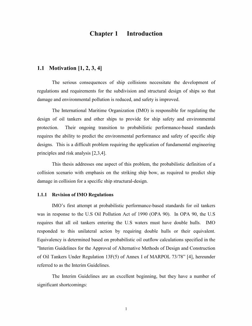
Figure 1.1 illustrates the process being used at Virginia Tech to predict
probabilistic damage as a function of ship structural design.
3
Struck ship design variables: Type (SH,DH,IOTD,DS,DB,DS) LBP, B, D Speed & displacement Subdivision Structural design
Probability given collision Point puncture, raking puncture, penetrating collision Pdf's: Striking ship speed Striking ship displacement Striking ship draft & bow height Striking ship bow shape and stiffness Collision striking location & angle
Monte Carlo Simulation
Extent of Damage
CalculationSpecificcollisionscenario's
Regression analysis
joint pdf for longitudinal, vertical and transverse extent of damage:
Pdf parametrics for extent of damage as a function of struck ship design
Figure 1.1 - Methodology to Predict Probabilistic Damage in Collision [1, 2]
The process begins with a set of probability density functions (pdfs) defining
possible collision scenarios. Based on these pdfs, a specific scenario is selected using a
Monte Carlo simulation, and combined with a specific ship structural design to predict
collision damage. This process is repeated for thousands of scenarios and a range of
structural designs until sufficient data is generated to build a set of parametric equations
relating probabilistic damage extent to structural design. These parametric equations can
then be used in oil outflow or damage stability calculations.
Critical to this process is a simple, but sufficient probabilistic definition of the
collision scenario, including the striking ship bow.
1.1.3 Collision Model for Probabilistic Analysis
The collision problem consists of two sub-problems:
• = External problem - includes the principal characteristics of the striking and struck
ships and their motion before, during and after collision;
• = Internal problem - includes the internal mechanics and structural response of the
struck ship and the striking ship bow during collision.
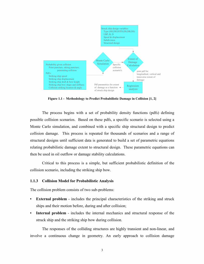
The responses of the colliding structures are highly transient and non-linear, and
involve a continuous change in geometry. An early approach to collision damage
4
evaluation was made by Minorsky [40, 57], who developed a simple linear relationship
between damaged structural volume and absorbed energy in collision, as illustrated in
Figure 1.2.
Minorsky Relationship(as modified by Reardon / Sprung)
0
2
4
6
8
10
12
14
0 100 200 300 400 500 600 700 800 900 1000
KE (MJ)
RT(m3)
Intercept - Shell Resistance
Slope - Hull Penetration
Figure 1.2 - Minorsky Model [40, 57]
SNAME Ad Hoc Panel #6 identified three types of side damage to consider, with
emphasis on penetrating collision:
• = Low energy puncture at point
• = Low energy raking puncture
• = Penetrating Collision – right angle and oblique sufficient to penetrate outer hull
with significant damage extending in at least 2 directions (penetration, horizontal,
vertical).
At Virginia Tech, initial work is focused on the penetrating collision using
SIMCOL (Simplified Collision Model) [17], a modified Minorsky collision model for
internal damage with three degree-of-freedom external ship dynamics. SIMCOL requires
a compatible striking ship definition, and collision scenarios that are simple, but
sufficient for accurate results.
5
Most of the existing theories for ship collisions assume that the bow of the
striking ship is infinitely stiff and that all energy-absorbing deformation occurs in the side
structure of the struck ship. The baseline collision model, SIMCOL Version 0.1, assumes:
• = Absorbed energy during crushing and tearing of internal structured can be
estimated using a “Modified Minorsky” method [40, 57].
• = 3 degrees of freedom (sway, yaw, surge) are required for both ships.
• = The striking ship bow is a rigid, vertically infinite wedge.
• = A membrane model can be used to estimate shell resistance (Van Mater, Jones, et.
al. - plastic membrane tension and rupture).
• = A fully coupled time-step solution is required.
The strengths of SIMCOL are:
• = Speed
• = Simple input
• = The ability to consider oblique collision angles and damage length.
Its limitations are:
• = Some structural details are not considered.
• = There is only limited data to define appropriate probabilistic scenarios.
• = The sufficiency of the striking ship bow model is suspect.
General improvements in SIMCOL are addressed in Chen [17]. This thesis examines the
sufficiency of the SIMCOL bow model. Questions examined in this thesis are:
• = Is it sufficient to assume that the striking ship bow is rigid?
• = Is the energy absorbed by the striking ship bow significant and does it vary in
different collision scenarios?
• = Is it sufficient to assume that the striking bow is an infinite wedge?
1.2 Hypothesis
The universal assumption of a rigid striking ship bow in ship collision analysis is
not valid. Differences in striking ship bow stiffness, draft, bow height and shape have an
6
important influence on the allocation of absorbed energy between striking and struck
ships and the extent of damage in the struck ship. The energy absorbed by the striking
ship can be significant and varies in different collision scenarios.
1.3 Plan
The scope of work in this thesis includes the development and validation of a
striking ship model that uses Pedersen's super-element approach [45,52] and the explicit
non-linear FE code LS-DYNA 3D [22, 23, 24] to simulate the bow collision event.
Important striking ship bow attributes, including a simplified striking ship sub-model for
use in future collision models are defined. Application of this bow model demonstrates
that the universal assumption of a rigid striking ship bow is not valid. Necessary tasks
include:
• = Identify necessary collision scenario variables [9, 63].
• = Propose a framework for defining the relationship of collision scenario variables,
and collect preliminary scenario data.
• = Describe and compare various bow models in the current literature.
• = Support the striking bow hypothesis using results from prior analysis.
• = Reproduce and compare closed-form load vs. indentation results by Amdahl [5, 6,
52], Yang and Caldwell [70, 52] and Pedersen [52] for four bow designs: (500
DWT coaster, 23K DWT container ship, 40K DWT container ship and 150K
DWT bulk carrier) striking a rigid wall at various speeds.
• = Create four coarse mesh "intersection" bow models (500 DWT coaster, 23K DWT
container ship, 40K DWT container ship and 150K DWT bulk carrier) in LS-
DYNA 3D using intersection and rigid elements. Review potential element
models and compare to available elements in LS-DYNA 3D. Run simulations of
bows striking a rigid wall at various speeds.
• = Create fine mesh, "conventional" bow models (23K DWT container ship and
150K DWT bulk carrier). Run simulations of bows striking a rigid wall at various
speeds.
7
• = Compare closed-form, "conventional" and "intersection" results for bows striking
a rigid wall at various speeds.
• = Create fine mesh "conventional" tanker side models (100K DWT SH tanker and
150K DWT DH tanker) in LS-DYNA. Run simulations of bow models striking
these stationary tankers and tankers with sway at various speeds.
• = Create coarse mesh "super-element" tanker side models (100K DWT SH tanker
and 150K DWT DH tanker) in LS-DYNA using super-elements. Run simulations
of bow models striking these stationary tankers and tankers with sway at various
speeds.
• = Compare "conventional" and "intersection" results for striking a tanker at various
speeds, with and without sway and propose a simplified bow model that
duplicates results to a reasonable accuracy level.
• = Propose a simplified and sufficient bow model.
1.4 Thesis Organization
After a survey of the literature and data available on ship collisions, data available
from various sources is compiled, organized and presented in Chapter 2. Chapter 2 also
proposes a sufficient set of collision scenario variables and a relationship framework.
Chapter 3 describes the theories behind various striking ship models developed by
different researchers. Chapter 4 shows that the energy absorbed by the striking ship bow
is significant and variable in a number of documented collision cases, and therefore needs
more examination.
Some of the salient features of LS-DYNA 3D and modeling techniques using
Finite Element Model Builder (FEMB) are discussed in Chapter 5. Chapter 6 describes
the finite element models developed using FEMB in more detail. The results from the
various simulations and calculations are analyzed and presented in Chapter 7. Chapter 8
discusses conclusions and suggested improvements for future work.
8
Chapter 2 Collision Scenarios and Data 2.1 Collision Scenario Variables
An important objective of this research is to specify a simplified, but sufficient
collision scenario definition for application in probabilistic collision analysis using
SIMCOL [17]. Although the primary emphasis of this thesis is to describe the striking
ship bow, this chapter discusses other scenario variables, proposes a framework for
defining their relationship, and provides preliminary scenario data. Variables considered
to describe the collision event include:
• = Struck ship random variables - all other characteristics of the struck ship are
design parameters and are not random variables
• = Speed
• = Trim
• = Displacement
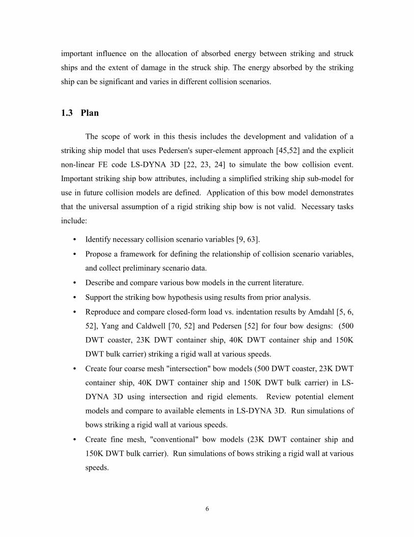
• = Event random variables – these variables are shown in Figure 2.1
• = Collision angle (φ)
• = Strike location (l)
• = Striking ship random variables
• = Speed
• = Displacement
• = Bow stiffness
• = Bow geometry – wedge or more detailed geometry
• = Half-angle
• = Bow extents: depth and draft at the bow
• = Other principal characteristics
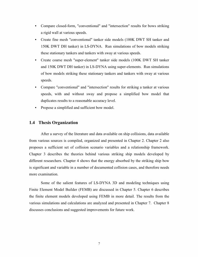
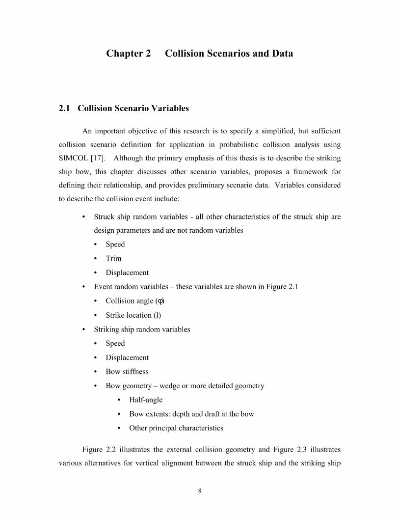
Figure 2.2 illustrates the external collision geometry and Figure 2.3 illustrates
various alternatives for vertical alignment between the struck ship and the striking ship
9
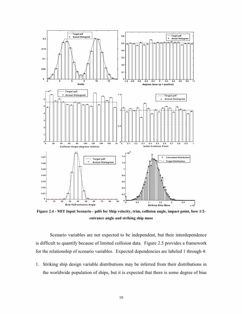
bow. Figure 2.4 shows probability density functions (pdfs) used in the earlier MIT study
[3].
x
y
è 1
ÑStriking Ship
Struck Ship
è2
l
Note: The positive direction of angle is alwayscounterclockwise.
G1
G2
Figure 2.1 - General Collision Scenario [1, 2]
Figure 2.2 - External Collision Geometry [53]
Figure 2.3 - Possible Variations of Striking Bow Geometry
10
Target pdfActual Histogram
2 4 6 8 10 120
0.05
0.1
0.15
0.2
knots
Target pdfActual Histogram
-0.8 -0.6 -0.4 -0.2 0 0.2 0.4 0.6 0.80
0.1
0.2
0.3
0.4
0.5
0.6
degrees (bow up = positive)-1.0 1.0
0 20 40 60 80 100 120 140 160 180
1
2
3
4
5
6
x 10-3
Collision Angle (degrees relative)
Target pdfActual Histogram
0 0.1 0.2 0 .3 0 .4 0 .5 0.6 0.7 0 .8 0 .9 10
0.5
1
1 .5
Initia l C ollision P oint
Target pdfActual H istogram
0 10 20 30 40 50 60 70 80 900
0.01
0.02
0.03
0.04
0.05
0.06
0.07
Bow Half-entrance Angle
Target pdfActual Histogram
0 0.5 1 1.5 2 2.5 3x 10⁵
0
0.2
0.4
0.6
0.8
1
1.2
1.4x 10⁻⁵
Striking Ship Mass
Calculated Distribution
Target Distribution
Figure 2.4 - MIT Input Scenario - pdfs for Ship velocity, trim, collision angle, impact point, bow 1/2-
entrance angle and striking ship mass
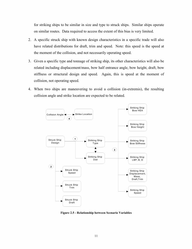
Scenario variables are not expected to be independent, but their interdependence
is difficult to quantify because of limited collision data. Figure 2.5 provides a framework
for the relationship of scenario variables. Expected dependencies are labeled 1 through 4:
1. Striking ship design variable distributions may be inferred from their distributions in
the worldwide population of ships, but it is expected that there is some degree of bias
11
for striking ships to be similar in size and type to struck ships. Similar ships operate
on similar routes. Data required to access the extent of this bias is very limited.
2. A specific struck ship with known design characteristics in a specific trade will also
have related distributions for draft, trim and speed. Note: this speed is the speed at
the moment of the collision, and not necessarily operating speed.
3. Given a specific type and tonnage of striking ship, its other characteristics will also be
related including displacement/mass, bow half entrance angle, bow height, draft, bow
stiffness or structural design and speed. Again, this is speed at the moment of
collision, not operating speed.
4. When two ships are maneuvering to avoid a collision (in-extremis), the resulting
collision angle and strike location are expected to be related.
Striking Ship Type
Striking Ship Dwt
Striking Ship Bow HEA
Striking Ship Bow Height
Striking Ship Bow Stiffness
Striking Ship LBP, B, D
Striking Ship Speed
Striking Ship Displacement,
Mass, Draft,Trim
Collision Angle Strike Location
Struck Ship Design
Struck Ship Speed
Struck Ship Trim
Struck Ship Draft
1
2
3
4
Figure 2.5 - Relationship between Scenario Variables
12
Even
t
Ship
nam
e and
type
Dead
weig
ht to
ns
Disp
lacem
ent t
ons
L.O.
A (ft
)
Brea
dth
(ft)
Dept
h (ft
)
Mean
Dra
ft (ft
)
Impa
ct A
ngle
(deg
rees
)
Dam
age L
engt
h (ft
)
Dam
age H
eight
(ft)
Spee
d (k
nots
)
Pene
tratio
n (ft
)
Passenger Liner Stockholm 4,700 16,500 525.2 69.1 38.50 24.6 30 29.0 18.0 Atlantic Ocean, Off
Nantucket Island, July 25, 1956 Passenger Liner
Andrea Doria 8,145 21,200 697.0 89.9 50.08 18.8
90
50 29.0 22.0 30
Tanker Arizona Standard 17,350 22,578 504.0 68.2 39.20 31.0 17 39.2 11.4 San Fransisco Bay
Entrance, January 18, 1971 Tanker Oregon
Standard 17,265 22,575 504.0 68.2 39.20 31.0
45
72 39.2 4.00 12
Passenger Royston Grange 10,385 14,660 489.0 65.7 35.3 22.5 110 30.0 13.0 Punta Indio
Channel, River Plate
May 11, 1972 Tanker Tien Chee 18,750 25,975 579.6 70.0 39.8 29.6
40
100 30.0 11.0 10
Tanker Oswedo Guardian 95,608 109,870 899.6 128 62 43.7 25.0 43.0 16.0
Off S. African Coast Between Alphard
Banks and Yzervarkpunt
August 21, 1972 Tanker Texanita 100,613 62,075 872.2 128 61.3 25.0
50
80.0 43.0 15.0 25
Containership C.V Sea Witch 16,343 26,670 610.0 78.2 54.5 27.3 21.0 36.0 15.5
New York Harbour June 2, 1973 Tanker Esso
Brussels 43,121 52,500 699.5 97.3 49.3 38.0
60
40.0 36.0 0.0 25
Tanker Stolt Viking 21,150 28,500 565.0 72.2 42.2 33.2 NIL NIL 12.0 Gulf of Mexico
January 7, 1978 Crewboat Candy Bar N/A 72 95.0 21.0 8.9 3.8
45 Cut in
half 8.9 14.0 21
General Cargo Santa Cruz II 20,373 25,855 520.0 74.0 44.0 32.5 Indent Indent 13.5
Chesapeake Bay, Mouth of the
Potomac River, Maryland
October 20, 1978 USCG Cutter
Cuyahoga N/A 460 125.0 24.0 18.0 10.0
5
15.0 10.0 11.3 10
Tanker Exxon Chester 29,210 36,630 627.9 82.7 42.5 33.6 31.0 40.0 10.0 Atlantic Ocean,
Sea of Cape Cod, June 18, 1979 Bulk Carrier Regal
Sword 27,464 34,714 576.9 75.0 48.6 36.0
60
150.0 25.0 12.0 20
Tanker Capricorn 24,796 29,950 604.9 75.2 41.8 31.5 Hawse pipe
Hawspipe 12.0
Tampa Bay, January 28, 1980 USCG Buoy tender
Blackthorn N/A 1,025 180.0 37.0 17.3 12.8
18 80.0 10.0 7.5 4
Chemical Tanker Coastal Transport 14,428 20,160 490.0 64.0 38.0 30.0 Bow to
frm 110 22.0 17.3 Lower Missisippi
River, Near Venice,
Louisiana November 24, 1980
Offshore Supply Sallee P N/A 395 115.0 26.0 8.0 7.0
90
34.0 8.0 14.0 20
Tanker Pisces 24,438 31,070 604.9 75.3 41.8 33.3 45.0 50.0 11.5 Missisippi River
December 27, 1980 Bulk Carrier Trade Master 33,448 41,768 628.3 86.9 50.2 37.0
90
55.0 50.0 11.1 18
Barge Carrier Lash Atlantico 29,820 44,606 819.8 100.2 60.0 32.1 70.0 30.0 18.0
Atlantic Ocean May 6, 1981 General Cargo
Hellenic Carrier 15,153 18,725 470.0 67.1 38.5 20.8
120
70.0 32.0 14.0 30
Barge Carrier Delta Norte 41,223 57,800 893.1 100.2 60.0 34.0 42.0 40.0 19.0
Gulf of Mexico, February 19, 1982 General Cargo
African Pioneer 12,391 18,600 495.0 71.4 39.7 18.3
45
80.0 33.0 15.0 30
13
Passenger / General Cargo
Yankee N/A 450 136.5 29.0 9.5 7.5 10.0 15.0 11.5
Rhode Island Sound July 2, 1983 General Cargo
Harbel Tapper N/A 17,525 435.0 72.0 35.0 26.5
70 Indent
only Indent only 5.0 0
Auto Carrier Figaro 27,764 35,894 649.6 105.9 102.4 29.8 72.0 70.0 10.0 Galveston Bay Entrance
November 10, 1988 Tanker Camargue 133,360 158,210 918.9 135.0 72.0 36.4
30
75.0 45.0 10.0 12
Bulk Carrier Atticos 29,165 17,176 593.1 75.9 47.6 15.1 Bulb 16.0 10.5 Lower Missisippi, March 24, 1993 Offshore Supply
Galveston N/A 630 180.0 40.0 14.3 8.2
120
15.0 14.3 13.5 12
Containership Hanjin Hongkong 20,000 27,780 796.6 105.6 62.3 17.1 55.0 62.3 10.0
Port Pusan May 2, 1994 Containership
President Washington
49,310 56,534 860.2 105.8 66.0 38.1
90
105.6 40.0 6.0 55
General Cargo Pacific Ares N/A 21,620 505.5 72.8 39.7 28.8 40.0 35.0 5.5 Bay of Tokyo,
Japan November 9, 1974 Tanker Yuyo Maru
No. 10 52,836 73,790 740.3 117.4 68.1 39.1 90
78.7 35.0 10.0 15
Tanker Texaco Iowa 41,282 53,850 699.5 97.0 49.0 38.6 30.0 1.0 8.0 Missisippi River, Pilottown, Louisiana
October 3, 1978 Tanker Burmah Spar 74,350 81,135 785.0 121.0 54.0 40.0
15 Indent only
Indent only 6.0 0
Bulk Carrier Maritime Justice 34,196 41,089 608.0 85.0 51.0 31.3 30.0 20.0 7.2
Lower Missisippi River, Near New
Orleans, Louisiana November 9, 1978
Bulk Carrier Irene S. Lemos 43,285 44,910 657.0 95.0 53.0 34.5
0 33.0 20.0 8.0 25
Tanker Mobil Vigilant 53,490 56,950 735.0 104.0 51.0 36.3 45.0 20.0 4.0 Neches River, Near
Beaumont, Texas February 25, 1979 Tanker Marine
Duval 24,734 34,224 612.0 80.0 42.0 33.4 42
160.0 20.0 6.6 18
Bulk Carrier Frotaleste 24,622 30,753 582.2 75.7 45.9 33.1 150.0 40.0 7.4
Lower Missisippi River, Near Bonnet
Carre Point, Louisiana
January 27, 1980 General Cargo
Cunene 16,311 18,050 522.7 69.5 44.1 25.0
135
22.0 40.0 0.0 12
Sternwheel passenger Natchez N/A 1,550 237.5 40.0 7.8 6.0 20.0 8.0 6.0
Under Greater New Orleans Bridge at
New Orleans, Louisiana,
March 29, 1980 Tanker Exxon
Baltimore 50,311 62,852 743.0 102.0 50.0 38.5
55
34.0 2.5 15.8 2.0
Bulk Carrier Sea Daniel N/A 28,300 551.2 75.0 46.4 32.0 35.0 30.0 6.0
Missisippi River, Gulf Outlet Near
Shell Beach, Louisiana
July 22, 1980 Containership Test
Bank N/A 18,060 467.5 68.9 35.5 28.0
45
45.0 30.0 4.0 10
Ferry Klahowya N/A 1,334 310.0 73.0 17.0 N/A 30.0 17.0 10.0 Seattle Harbor, Washington D.C
Jan 13, 1981 General Cargo / Vehicle freighter
Sankograin 20,138 13,570 514.0 75.0 44.3 19.2
40 Indent
only Indent only 2.0 0
General Cargo Hoegh Orchid 18,207 26,450 599.8 67.7 41.3 30.8 6.5 6.0 4.0 Upper New York
Bay May 6, 1981 Ferry American
Legion N/A 5,025 294.0 69.0 20.6 14.3 90
9.0 50.0 2.0 15
Tanker Maersk Neptune 68,800 85,100 811.0 105.5 57.1 43.2 Bow
indent Bow
indent 1.5 Upper New York
Bay – Feb 18, 1988 Bulk Carrier Mont Fort 26,748 34,868 600.6 73.7 46.6 34.5
45
16.0 34.0 0.0 10
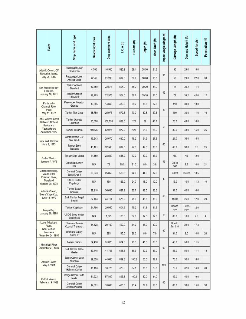
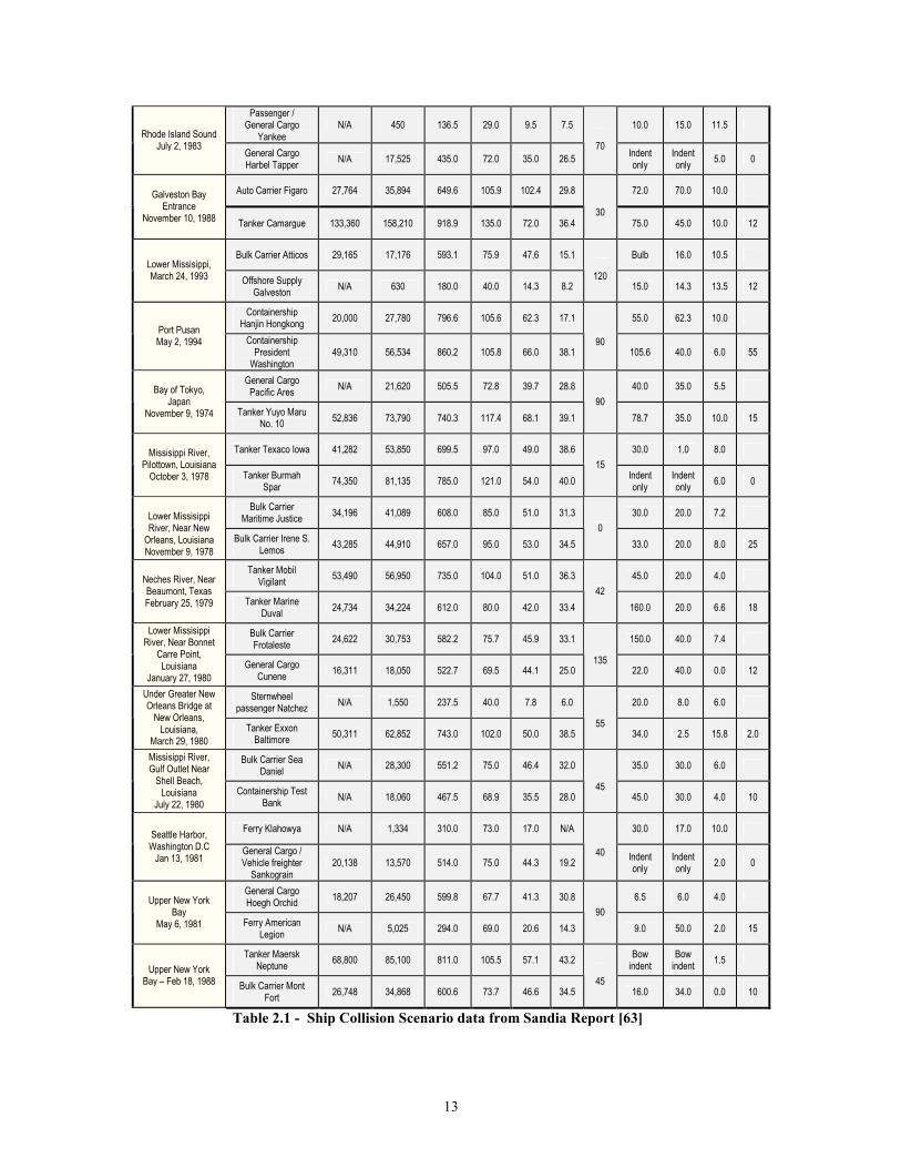
Table 2.1 - Ship Collision Scenario data from Sandia Report [63]
14
The relationships shown in Figure 2.5 require data to quantify, and this data is
very limited and/or difficult to obtain.
Table 2.1 presents data available on various collisions that took place between
1979 and 1993 [63]. The information presented is derived from various sources,
including the Sandia report [63]. This data may be used together with worldwide ship
data to quantify the relationships shown in Figure 2.5. This will be accomplished in
future work.
2.2 Rigid Bow Geometry
This section compares the geometry of the striking ships used in DAMAGE, the
DTU model, ALPS/SCOL and SIMCOL.
Both DAMAGE and the DTU model calculate the absorbed energy for direct
contact deformation of struck ship super-elements by the striking ship bow. This is not a
finite element method. Deformation away from the actual striking ship penetration is not
considered. Both methods are based on the same deformation and energy evaluation
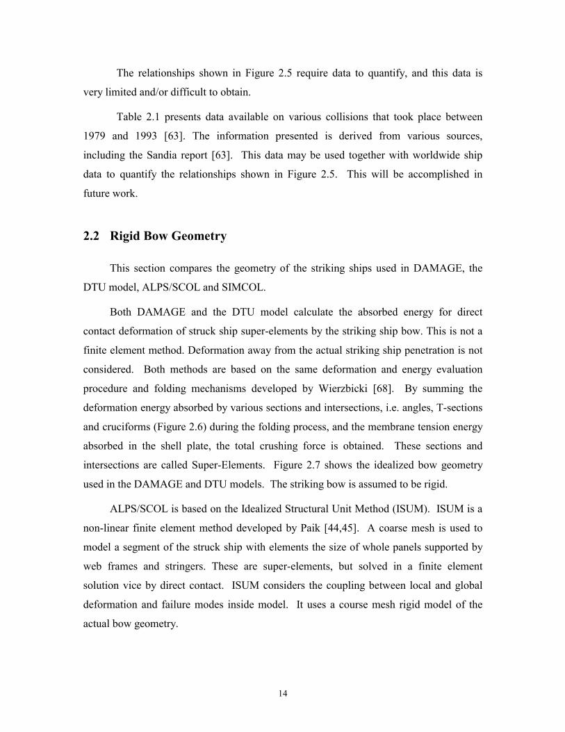
procedure and folding mechanisms developed by Wierzbicki [68]. By summing the
deformation energy absorbed by various sections and intersections, i.e. angles, T-sections
and cruciforms (Figure 2.6) during the folding process, and the membrane tension energy
absorbed in the shell plate, the total crushing force is obtained. These sections and
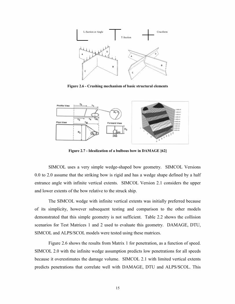
intersections are called Super-Elements. Figure 2.7 shows the idealized bow geometry
used in the DAMAGE and DTU models. The striking bow is assumed to be rigid.
ALPS/SCOL is based on the Idealized Structural Unit Method (ISUM). ISUM is a
non-linear finite element method developed by Paik [44,45]. A coarse mesh is used to
model a segment of the struck ship with elements the size of whole panels supported by
web frames and stringers. These are super-elements, but solved in a finite element
solution vice by direct contact. ISUM considers the coupling between local and global
deformation and failure modes inside model. It uses a course mesh rigid model of the
actual bow geometry.
15
L-Section or Angle
T-Section
Cruciform
Figure 2.6 - Crushing mechanism of basic structural elements
Figure 2.7 - Idealization of a bulbous bow in DAMAGE [62]
SIMCOL uses a very simple wedge-shaped bow geometry. SIMCOL Versions
0.0 to 2.0 assume that the striking bow is rigid and has a wedge shape defined by a half
entrance angle with infinite vertical extents. SIMCOL Version 2.1 considers the upper
and lower extents of the bow relative to the struck ship.
The SIMCOL wedge with infinite vertical extents was initially preferred because
of its simplicity, however subsequent testing and comparison to the other models
demonstrated that this simple geometry is not sufficient. Table 2.2 shows the collision
scenarios for Test Matrices 1 and 2 used to evaluate this geometry. DAMAGE, DTU,
SIMCOL and ALPS/SCOL models were tested using these matrices.
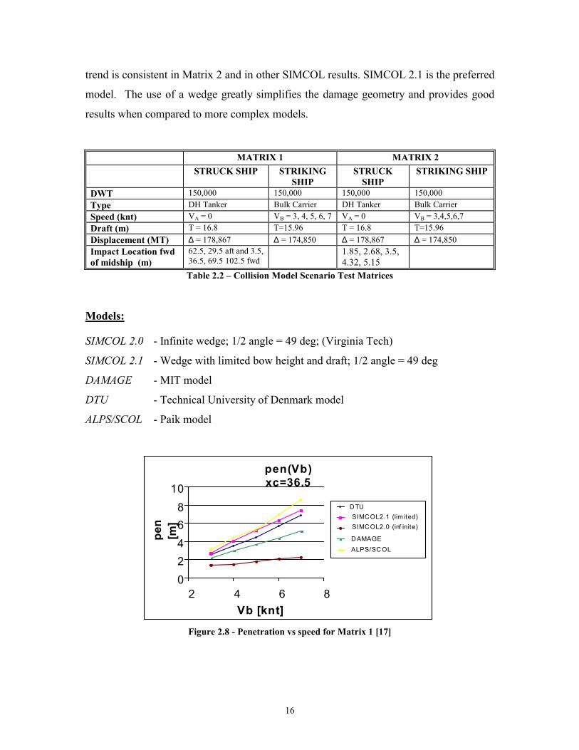
Figure 2.6 shows the results from Matrix 1 for penetration, as a function of speed.
SIMCOL 2.0 with the infinite wedge assumption predicts low penetrations for all speeds
because it overestimates the damage volume. SIMCOL 2.1 with limited vertical extents
predicts penetrations that correlate well with DAMAGE, DTU and ALPS/SCOL. This
16
trend is consistent in Matrix 2 and in other SIMCOL results. SIMCOL 2.1 is the preferred
model. The use of a wedge greatly simplifies the damage geometry and provides good
results when compared to more complex models.
MATRIX 1 MATRIX 2 STRUCK SHIP STRIKING
SHIP STRUCK
SHIP STRIKING SHIP
DWT 150,000 150,000 150,000 150,000 Type DH Tanker Bulk Carrier DH Tanker Bulk Carrier Speed (knt) VA = 0 VB = 3, 4, 5, 6, 7 VA = 0 VB = 3,4,5,6,7 Draft (m) T = 16.8 T=15.96 T = 16.8 T=15.96 Displacement (MT) ∆ = 178,867 ∆ = 174,850 ∆ = 178,867 ∆ = 174,850 Impact Location fwd of midship (m)
62.5, 29.5 aft and 3.5, 36.5, 69.5 102.5 fwd
1.85, 2.68, 3.5, 4.32, 5.15
Table 2.2 – Collision Model Scenario Test Matrices
Models:
SIMCOL 2.0 - Infinite wedge; 1/2 angle = 49 deg; (Virginia Tech)
SIMCOL 2.1 - Wedge with limited bow height and draft; 1/2 angle = 49 deg
DAMAGE - MIT model
DTU - Technical University of Denmark model
ALPS/SCOL - Paik model
pen(Vb) xc=36.5
0 2 4 6 8
10
2 4 6 8 Vb [knt]
pen
[m]
D TU SIMCOL2.1 (lim ited) SIMCOL2.0 (inf inite) D AMAGE ALPS/SC OL
Figure 2.8 - Penetration vs speed for Matrix 1 [17]
17
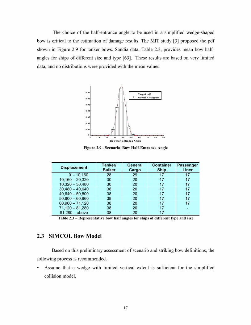
The choice of the half-entrance angle to be used in a simplified wedge-shaped
bow is critical to the estimation of damage results. The MIT study [3] proposed the pdf
shown in Figure 2.9 for tanker bows. Sandia data, Table 2.3, provides mean bow half-
angles for ships of different size and type [63]. These results are based on very limited
data, and no distributions were provided with the mean values.
0 10 20 30 40 50 60 70 80 900
0.01
0.02
0.03
0.04
0.05
0.06
0.07
Bow Half-entrance Angle
Target pdfActual H istogram
Figure 2.9 - Scenario–Bow Half-Entrance Angle
Displacement Tanker/ Bulker
General Cargo
Container Ship
Passenger Liner
0 - 10,160 28 29 17 17 10,160 – 20,320 30 20 17 17 10,320 – 30,480 30 20 17 17 30,480 – 40,640 38 20 17 17 40,640 – 50,800 38 20 17 17 50,800 – 60,960 38 20 17 17 60,960 – 71,120 38 20 17 17 71,120 – 81,280 38 20 17 - 81,280 – above 38 20 17 -
Table 2.3 – Representative bow half angles for ships of different type and size
2.3 SIMCOL Bow Model
Based on this preliminary assessment of scenario and striking bow definitions, the
following process is recommended.
• = Assume that a wedge with limited vertical extent is sufficient for the simplified
collision model.
18
• = Continue to collect and analyze statistical collision data for collision angle and strike
location. Propose pdf(s) for these variables. Use the MIT pdfs in Figure 2.4 as the
baseline definition.
• = Define striking ship characteristics using the relationships proposed in Figure 2.5.
Use worldwide ship data to define the baseline distributions, and modify these when
actual collision data or ship encounter data is available and sufficient.
• = Analyze the structural design and stiffness of the striking ship bow and propose a
simplified relationship between bow penetration and force for application in
SIMCOL.
The remainder of this thesis will focus on bow models, with emphasis on bow stiffness.
19
Chapter 3 Bow Damage Models 3.1 INTRODUCTION
This chapter describes bow models developed by various researchers. A brief
overview of each model is presented. There are two main types of bow models: rigid and
deformable. Although Minorsky [40] considers bow deformation, extensions of his
theory typically use a rigid bow. Because of this, Minorsky’s model is presented
separately in Section 3.2. Rigid bow models are described in Section 3.3 and Section 3.4
describes deformable bow models. A summary table is provided in Section 3.5.
3.2 Minorsky [40]
Minorsky’s work is among the earliest in the field of ship collisions. Minorsky
examined fifty major collision cases that occurred before 1959. He developed an
empirical “Resistance Factor” for predicting energy absorption based on the volume of
damaged steel components in the striking and struck ships, and correlated it with the
absorbed kinetic energy causing major damage.
Since an attempt to produce an analytical solution would of necessity rest on
many doubtful assumptions, Minorsky preferred to follow a semi-empirical approach
based on the data from 50 actual collisions, which were supplied by the U.S Coast Guard.
The data included speeds, angles of encounter, displacements, drafts and extents and
location of damage. Of these collisions, those with very oblique collision angles were
eliminated.
The twenty-six cases remaining were analyzed for absorbed kinetic energy and
extent of damage. As only right-angle penetration is calculated, only velocity
components normal to the struck ship’s centerline are considered. The effect of the added
mass of water dm and the ratio (R = MB/MA) of the mass of the striking ship (MB) to that
20
of the struck ship (MA) is considered. A coefficient of energy absorption, K is defined as
a function of MA, MB and dm.
K M dmM M dm
A
B A
= ++ +
(3.1)
Where:
K is the percentage of the initial kinetic energy in the direction normal to the struck ship’s
centerline that is absorbed in the collision.
When R → 0, i.e, when the striking ship is very small compared to the struck
ship, K → 1and most of the initial kinetic energy normal to the struck ship’s centerline is
absorbed in the collision. When R → ∞, the case where a very large vessel strikes a small
shallow draft vessel, K → 0, and the small vessel is pushed away without absorbing
significant kinetic energy.
Based on the assumption of a wholly inelastic impact, the absorbed kinetic energy
is expressed as a function of the displacements of the colliding vessels, velocity of the
striking ship (VB) and angle of impact (θ) [40]:
2)(243.1
θSinV BBB
BA
∆+∆
∆∆ (3.2)
Where:
∆A is the displacement of the struck ship;
∆B is the displacement of the striking ship
Those members having little depth in the direction of penetration, such as the
shell of the struck ship, do not contribute to the resistance factor. Members having depth
in the direction of penetration, such as decks, transverses, flats and inner and outer
bottoms of both vessels and the shell of the striking ship, are considered. A resistance
factor, RT is calculated based on damage to the following structural members:
• = Decks, flats and double bottoms in both struck and striking vessels
• = Transverse bulkheads in struck vessel
• = Longitudinal bulkheads in striking vessel
21
• = The component in the direction of collision of the shell of the striking vessel
(assumed at 0.7 of shell area)
The resistance factor is given by the equation:
nnnNNNT tLPtLPR += (3.3)
Where:
PN is the depth of damage in the Nth member of the striking vessel;
LN is the length of damage in the Nth member of the striking vessel;
tN is the thickness of the Nth member of the striking vessel;
Pn is the depth of damage in the nth member of the struck vessel;
Ln is the length of damage in the nth member of the struck vessel;
tn is the thickness of the nth member of the struck vessel
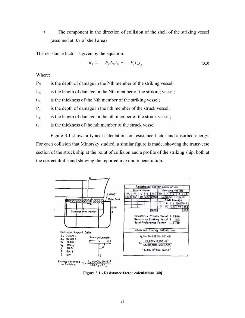
Figure 3.1 shows a typical calculation for resistance factor and absorbed energy.
For each collision that Minorsky studied, a similar figure is made, showing the transverse
section of the struck ship at the point of collision and a profile of the striking ship, both at
the correct drafts and showing the reported maximum penetration.
Figure 3.1 - Resistance factor calculations [40]
22
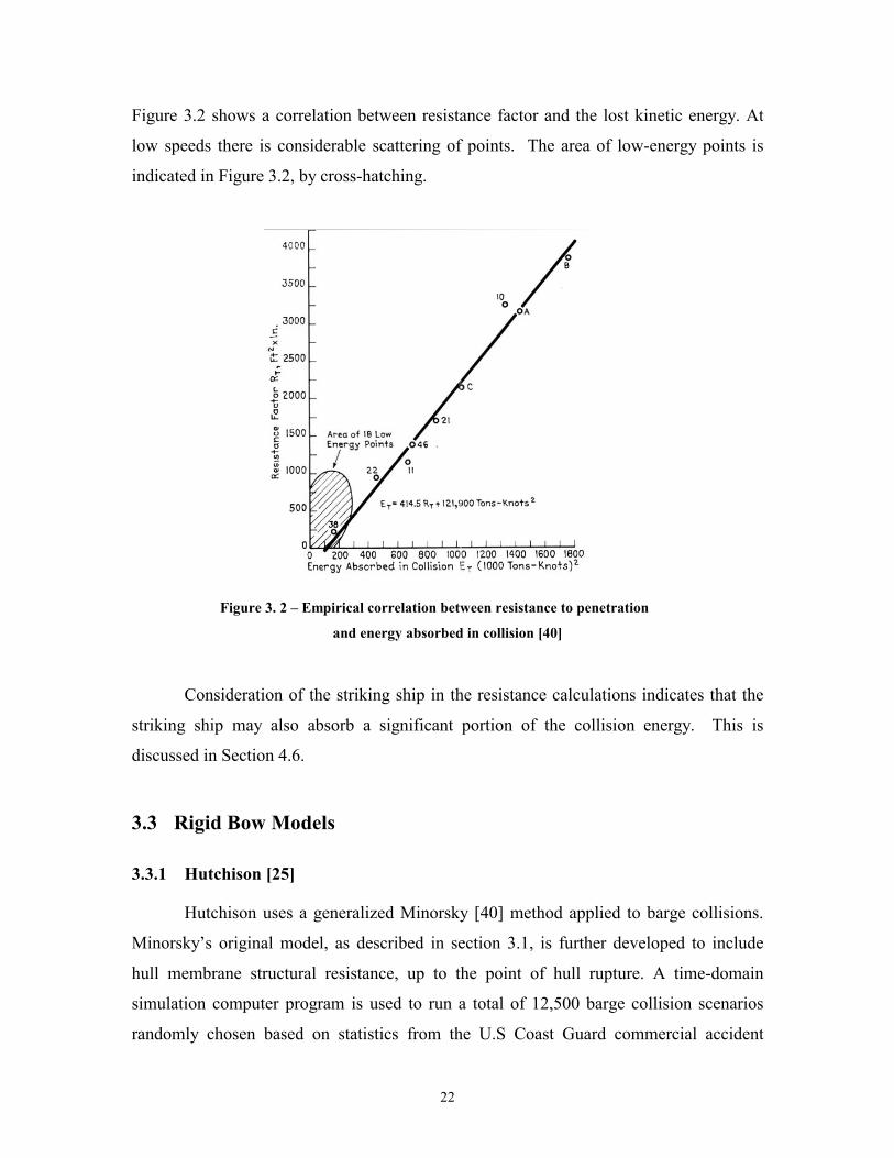
Figure 3.2 shows a correlation between resistance factor and the lost kinetic energy. At
low speeds there is considerable scattering of points. The area of low-energy points is
indicated in Figure 3.2, by cross-hatching.
Figure 3. 2 – Empirical correlation between resistance to penetration
and energy absorbed in collision [40]
Consideration of the striking ship in the resistance calculations indicates that the
striking ship may also absorb a significant portion of the collision energy. This is
discussed in Section 4.6.
3.3 Rigid Bow Models
3.3.1 Hutchison [25]
Hutchison uses a generalized Minorsky [40] method applied to barge collisions.
Minorsky’s original model, as described in section 3.1, is further developed to include
hull membrane structural resistance, up to the point of hull rupture. A time-domain
simulation computer program is used to run a total of 12,500 barge collision scenarios
randomly chosen based on statistics from the U.S Coast Guard commercial accident
23
database. Distributions are estimated for: 1) collision energy absorbed; 2) penetration; 3)
peak acceleration, and whether or not the hull membrane is ruptured.
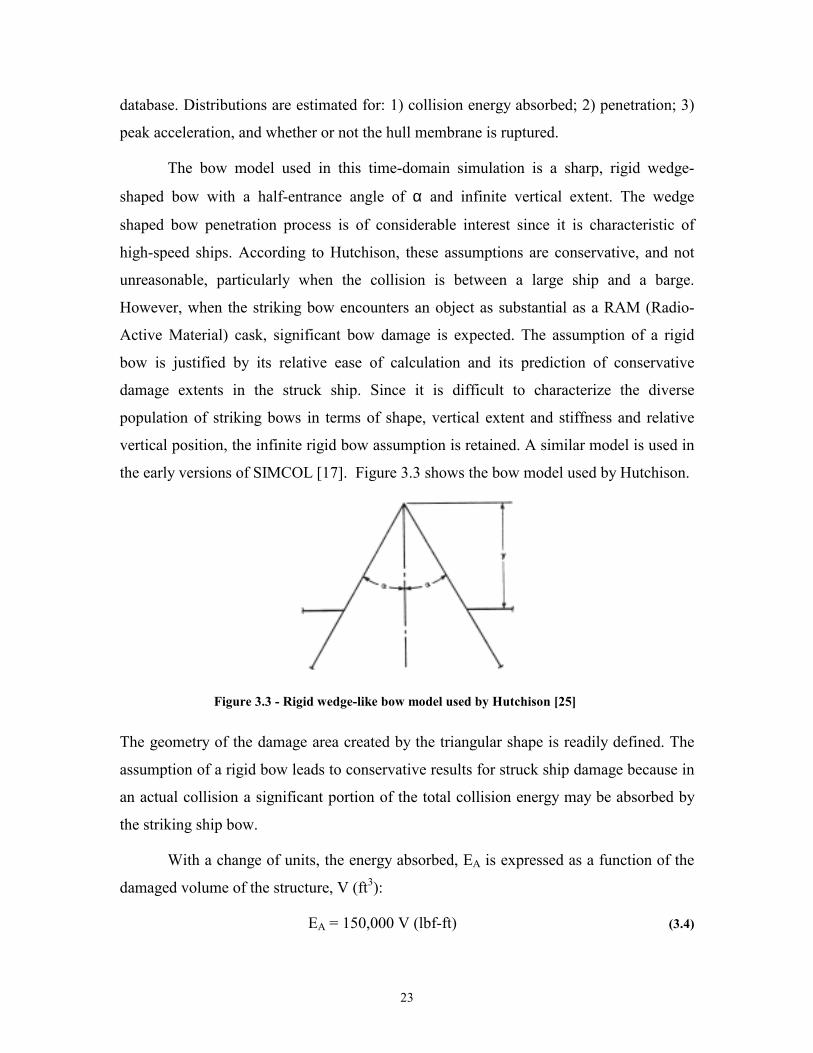
The bow model used in this time-domain simulation is a sharp, rigid wedge-
shaped bow with a half-entrance angle of α and infinite vertical extent. The wedge
shaped bow penetration process is of considerable interest since it is characteristic of
high-speed ships. According to Hutchison, these assumptions are conservative, and not
unreasonable, particularly when the collision is between a large ship and a barge.
However, when the striking bow encounters an object as substantial as a RAM (Radio-
Active Material) cask, significant bow damage is expected. The assumption of a rigid
bow is justified by its relative ease of calculation and its prediction of conservative
damage extents in the struck ship. Since it is difficult to characterize the diverse
population of striking bows in terms of shape, vertical extent and stiffness and relative
vertical position, the infinite rigid bow assumption is retained. A similar model is used in
the early versions of SIMCOL [17]. Figure 3.3 shows the bow model used by Hutchison.
Figure 3.3 - Rigid wedge-like bow model used by Hutchison [25]
The geometry of the damage area created by the triangular shape is readily defined. The
assumption of a rigid bow leads to conservative results for struck ship damage because in
an actual collision a significant portion of the total collision energy may be absorbed by
the striking ship bow.
With a change of units, the energy absorbed, EA is expressed as a function of the
damaged volume of the structure, V (ft3):
EA = 150,000 V (lbf-ft) (3.4)
24
The penetrated structure is assumed to have a composite thickness of t. The
energy absorbed in deforming the structure is dE = dW = Fdu = 150,000 V = 150,000 t
dw du. So the damaged material volume up to any penetration distance, y, is:
E y ty( ) , tan( )=150 000 2 α (3.5)
and the force acting in the negative y-direction to oppose the penetration is:
F y ty( ) [ , tan( )]= 2 150 000 α (3.6)
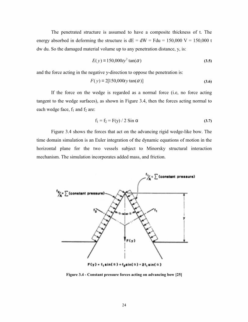
If the force on the wedge is regarded as a normal force (i.e, no force acting
tangent to the wedge surfaces), as shown in Figure 3.4, then the forces acting normal to
each wedge face, f1 and f2 are:
f1 = f2 = F(y) / 2 Sin α (3.7)
Figure 3.4 shows the forces that act on the advancing rigid wedge-like bow. The
time domain simulation is an Euler integration of the dynamic equations of motion in the
horizontal plane for the two vessels subject to Minorsky structural interaction
mechanism. The simulation incorporates added mass, and friction.
Figure 3.4 - Constant pressure forces acting on advancing bow [25]
25
3.3.2 Ito [27]
Ito investigates the effects of various design parameters on the strength of double-
hulled structures in collision. The collisions are classified into five types, two of which
are examined, one where a stem collides against the ship’s side and the other where a
bulbous bow collides against it. Static destruction tests are carried out using a series of
double hull models, which cover a wide strength-distribution range. Two different bow
models, one using the stem of the bow and the other using the bulb are created and tested.
Model tests are performed and used to validate calculated results. The stem and the bulb
used in the calculations are assumed rigid.
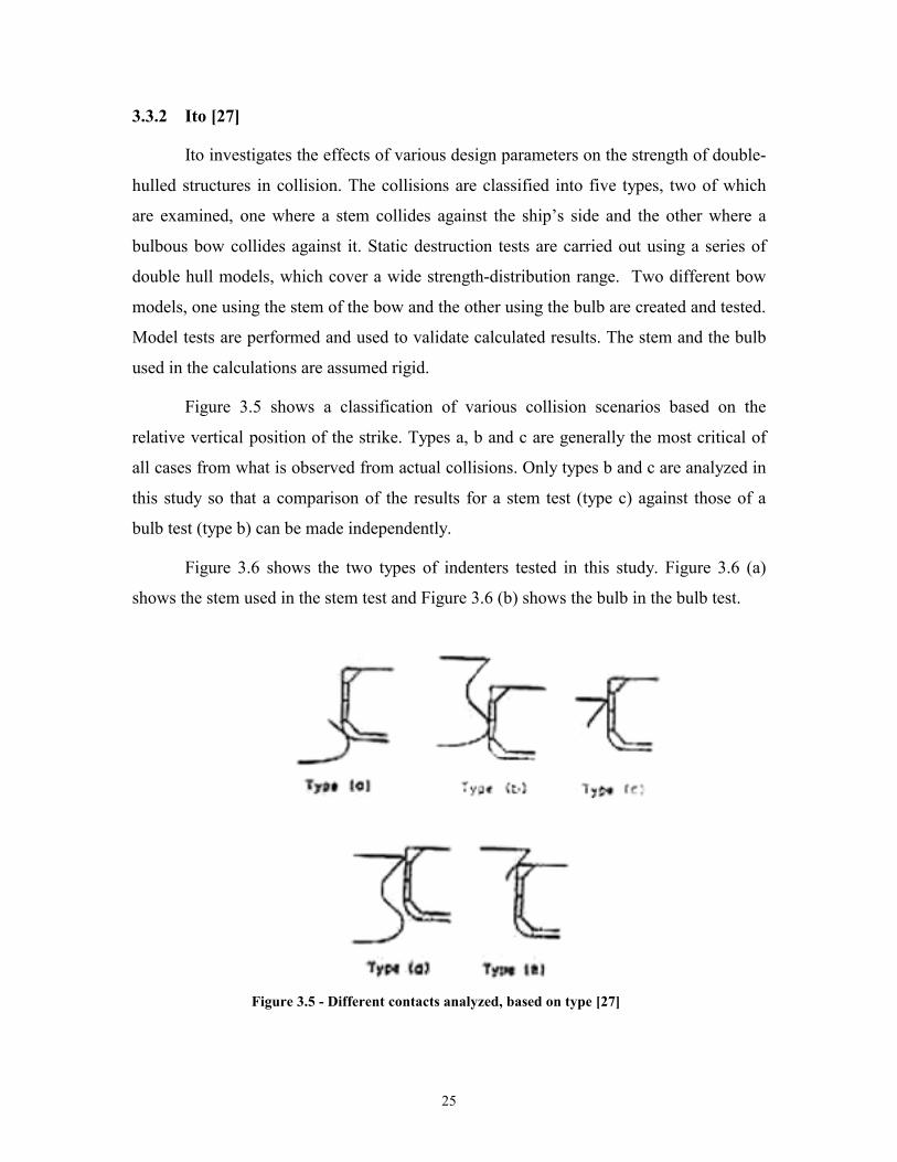
Figure 3.5 shows a classification of various collision scenarios based on the
relative vertical position of the strike. Types a, b and c are generally the most critical of
all cases from what is observed from actual collisions. Only types b and c are analyzed in
this study so that a comparison of the results for a stem test (type c) against those of a
bulb test (type b) can be made independently.
Figure 3.6 shows the two types of indenters tested in this study. Figure 3.6 (a)
shows the stem used in the stem test and Figure 3.6 (b) shows the bulb in the bulb test.
Figure 3.5 - Different contacts analyzed, based on type [27]

26
Figure 3.6 - Rigid bow model used by Ito [27]
Figure 3.7 shows the double hull ship used in the experiments. As can be seen
from the figure, the ship model is very coarse, without much detail. The collision point is
midway between two transverse bulkheads along the centerline of the two side stringers.
The bow models are gradually pushed into the double-hulled structure using a hydraulic
jack. Measurements of load, penetration, deformation and strain are made.
Figure 3.7 - The two types of experiments performed by Ito [27]
The assumptions made in the analysis are as follows:
• = The striking bow is rigid
• = Collisions are right-angled
• = The double-hulled structure is damaged only in the vicinity of the point of contact. It
does not collapse in its entirety.
• = When the bow strikes the side shell of the double-hulled structure, the side shell
behaves as a plastic membrane. Transverse webs and stringers are buckling members.
• = The damage penetration does not extend beyond the inner hull
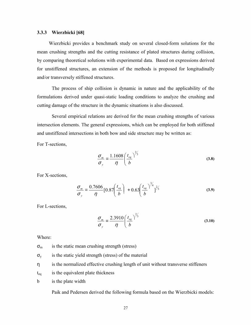
27
3.3.3 Wierzbicki [68]
Wierzbicki provides a benchmark study on several closed-form solutions for the
mean crushing strengths and the cutting resistance of plated structures during collision,
by comparing theoretical solutions with experimental data. Based on expressions derived
for unstiffened structures, an extension of the methods is proposed for longitudinally
and/or transversely stiffened structures.
The process of ship collision is dynamic in nature and the applicability of the
formulations derived under quasi-static loading conditions to analyze the crushing and
cutting damage of the structure in the dynamic situations is also discussed.
Several empirical relations are derived for the mean crushing strengths of various
intersection elements. The general expressions, which can be employed for both stiffened
and unstiffened intersections in both bow and side structure may be written as:
For T-sections,
32
1608.1 ����
�=
bteq
y
m
ησσ (3.8)
For X-sections,
324
3
]63.087.0[7606.0 ����
�+��
����
�=
bt
bt eqeq
y
m
ησσ (3.9)
For L-sections,
32
3910.2 ����
�=
bteq
y
m
ησσ (3.10)
Where:
σm is the static mean crushing strength (stress)
σy is the static yield strength (stress) of the material
η= is the normalized effective crushing length of unit without transverse stiffeners
teq is the equivalent plate thickness
b is the plate width
Paik and Pedersen derived the following formula based on the Wierzbicki models:
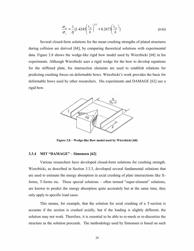
28
]2673.04245.1[15.0
����
�+��
����
�=
bt
bt eqeq
y
m
ησσ (3.11)
Several closed-form solutions for the mean crushing strengths of plated structures
during collision are derived [68], by comparing theoretical solutions with experimental
data. Figure 3.8 shows the wedge-like rigid bow model used by Wierzbicki [68] in his
experiments. Although Wierzbicki uses a rigid wedge for the bow to develop equations
for the stiffened plate, his intersection elements are used to establish relations for
predicting crushing forces on deformable bows. Wierzbicki’s work provides the basis for
deformable bows used by other researchers. His experiments and DAMAGE [62] use a
rigid bow.
Figure 3.8 – Wedge-like Bow model used by Wierzbicki [68]
3.3.4 MIT “DAMAGE” – Simonsen [62]
Various researchers have developed closed-form solutions for crushing strength.
Wierzbicki, as described in Section 3.3.3, developed several fundamental solutions that
are used to estimate the energy absorption in axial crushing of plate intersections like X-
forms, T-forms etc. These special solutions – often termed “super-element” solutions,
are known to predict the energy absorption quite accurately but at the same time, they
only apply to specific load cases.
This means, for example, that the solution for axial crushing of a T-section is
accurate if the section is crushed axially, but if the loading is slightly different, the
solution may not work. Therefore, it is essential to be able to re-mesh or re-discretize the
structure as the solution proceeds. The methodology used by Simonsen is based on such
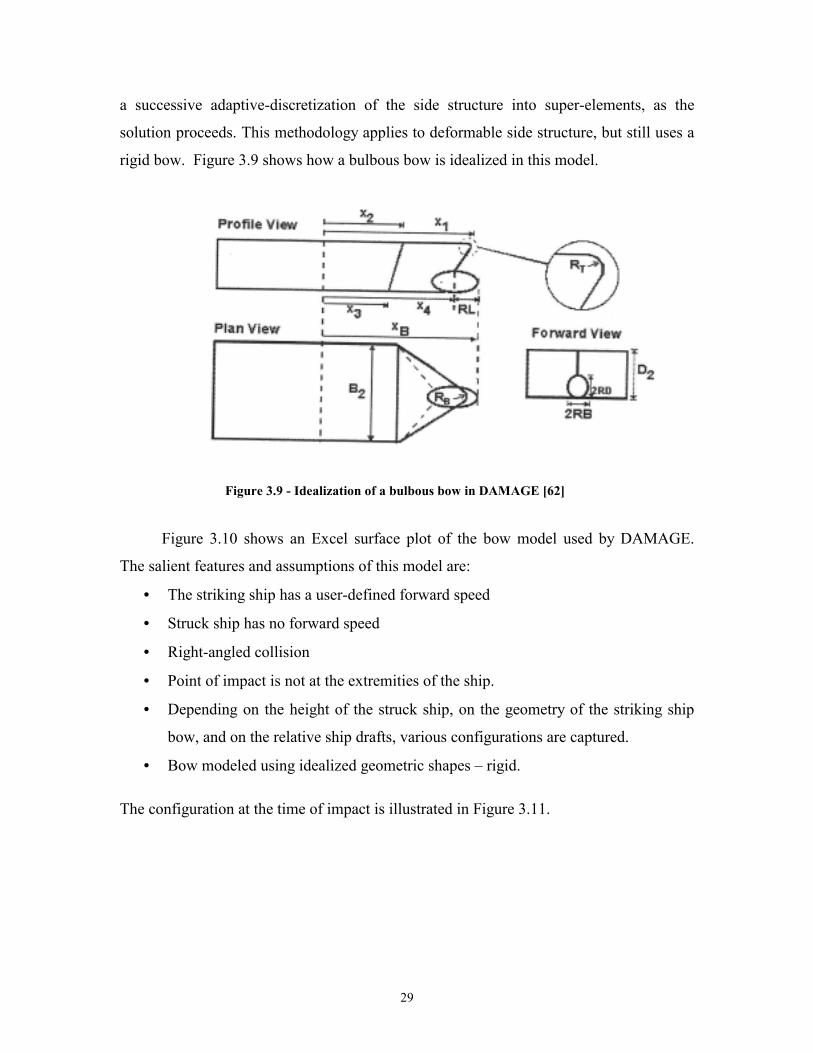
29
a successive adaptive-discretization of the side structure into super-elements, as the
solution proceeds. This methodology applies to deformable side structure, but still uses a
rigid bow. Figure 3.9 shows how a bulbous bow is idealized in this model.
Figure 3.9 - Idealization of a bulbous bow in DAMAGE [62]
Figure 3.10 shows an Excel surface plot of the bow model used by DAMAGE.
The salient features and assumptions of this model are:
• = The striking ship has a user-defined forward speed
• = Struck ship has no forward speed
• = Right-angled collision
• = Point of impact is not at the extremities of the ship.
• = Depending on the height of the struck ship, on the geometry of the striking ship
bow, and on the relative ship drafts, various configurations are captured.
• = Bow modeled using idealized geometric shapes – rigid.
The configuration at the time of impact is illustrated in Figure 3.11.
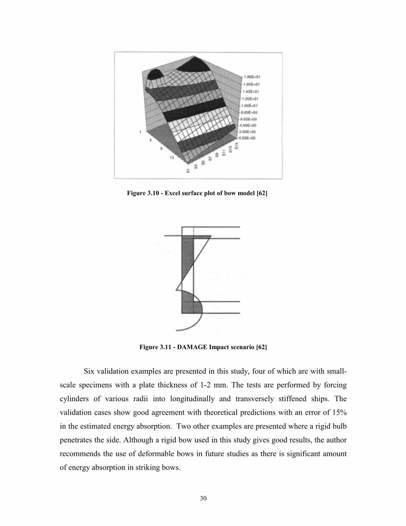
30
Figure 3.10 - Excel surface plot of bow model [62]
Figure 3.11 - DAMAGE Impact scenario [62]
Six validation examples are presented in this study, four of which are with small-
scale specimens with a plate thickness of 1-2 mm. The tests are performed by forcing
cylinders of various radii into longitudinally and transversely stiffened ships. The
validation cases show good agreement with theoretical predictions with an error of 15%
in the estimated energy absorption. Two other examples are presented where a rigid bulb
penetrates the side. Although a rigid bow used in this study gives good results, the author
recommends the use of deformable bows in future studies as there is significant amount
of energy absorption in striking bows.
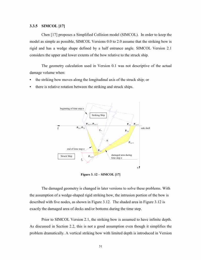
31
3.3.5 SIMCOL [17]
Chen [17] proposes a Simplified Collision model (SIMCOL). In order to keep the
model as simple as possible, SIMCOL Versions 0.0 to 2.0 assume that the striking bow is
rigid and has a wedge shape defined by a half entrance angle. SIMCOL Version 2.1
considers the upper and lower extents of the bow relative to the struck ship.
The geometry calculation used in Version 0.1 was not descriptive of the actual
damage volume when:
• = the striking bow moves along the longitudinal axis of the struck ship; or
• = there is relative rotation between the striking and struck ships.
beginning of time step n
end of time step n
damaged area duringtime step n
η
Striking Ship
Struck Ship
ξ side shellP4,n, P5,n
P4,n+1, P5,n+1 P1,n P1,n+1
P2,n
P2,n+1
P3,n+1
P3,n
φ′n
α
ζn
Figure 3. 12 – SIMCOL [17]
The damaged geometry is changed in later versions to solve these problems. With
the assumption of a wedge-shaped rigid striking bow, the intrusion portion of the bow is
described with five nodes, as shown in Figure 3.12. The shaded area in Figure 3.12 is
exactly the damaged area of decks and/or bottoms during the time step.
Prior to SIMCOL Version 2.1, the striking bow is assumed to have infinite depth.
As discussed in Section 2.2, this is not a good assumption even though it simplifies the
problem dramatically. A vertical striking bow with limited depth is introduced in Version
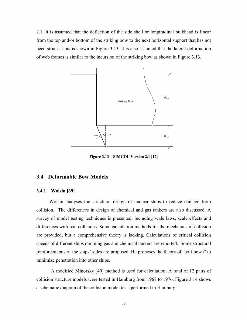
32
2.1. It is assumed that the deflection of the side shell or longitudinal bulkhead is linear
from the top and/or bottom of the striking bow to the next horizontal support that has not
been struck. This is shown in Figure 3.13. It is also assumed that the lateral deformation
of web frames is similar to the incursion of the striking bow as shown in Figure 3.13.
Striking Bow
è btm Bbtm
Bdep
Figure 3.13 – SIMCOL Version 2.1 [17]
3.4 Deformable Bow Models
3.4.1 Woisin [69]
Woisin analyses the structural design of nuclear ships to reduce damage from
collision. The differences in design of chemical and gas tankers are also discussed. A
survey of model testing techniques is presented, including scale laws, scale effects and
differences with real collisions. Some calculation methods for the mechanics of collision
are provided, but a comprehensive theory is lacking. Calculations of critical collision
speeds of different ships ramming gas and chemical tankers are reported. Some structural
reinforcements of the ships’ sides are proposed. He proposes the theory of “soft bows” to
minimize penetration into other ships.
A modified Minorsky [40] method is used for calculation. A total of 12 pairs of
collision structure models were tested in Hamburg from 1967 to 1976. Figure 3.14 shows
a schematic diagram of the collision model tests performed in Hamburg.
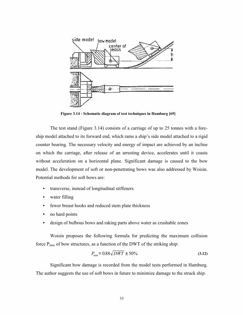
33
Figure 3.14 - Schematic diagram of test techniques in Hamburg [69]
The test stand (Figure 3.14) consists of a carriage of up to 25 tonnes with a fore-
ship model attached to its forward end, which rams a ship’s side model attached to a rigid
counter bearing. The necessary velocity and energy of impact are achieved by an incline
on which the carriage, after release of an arresting device, accelerates until it coasts
without acceleration on a horizontal plane. Significant damage is caused to the bow
model. The development of soft or non-penetrating bows was also addressed by Woisin.
Potential methods for soft bows are:
• = transverse, instead of longitudinal stiffeners
• = water filling
• = fewer breast hooks and reduced stem plate thickness
• = no hard points
• = design of bulbous bows and raking parts above water as crushable zones
Woisin proposes the following formula for predicting the maximum collision
force Pmax of bow structures, as a function of the DWT of the striking ship:
P DWTmax .= ±0 88 50% (3.12)
Significant bow damage is recorded from the model tests performed in Hamburg.
The author suggests the use of soft bows in future to minimize damage to the struck ship.
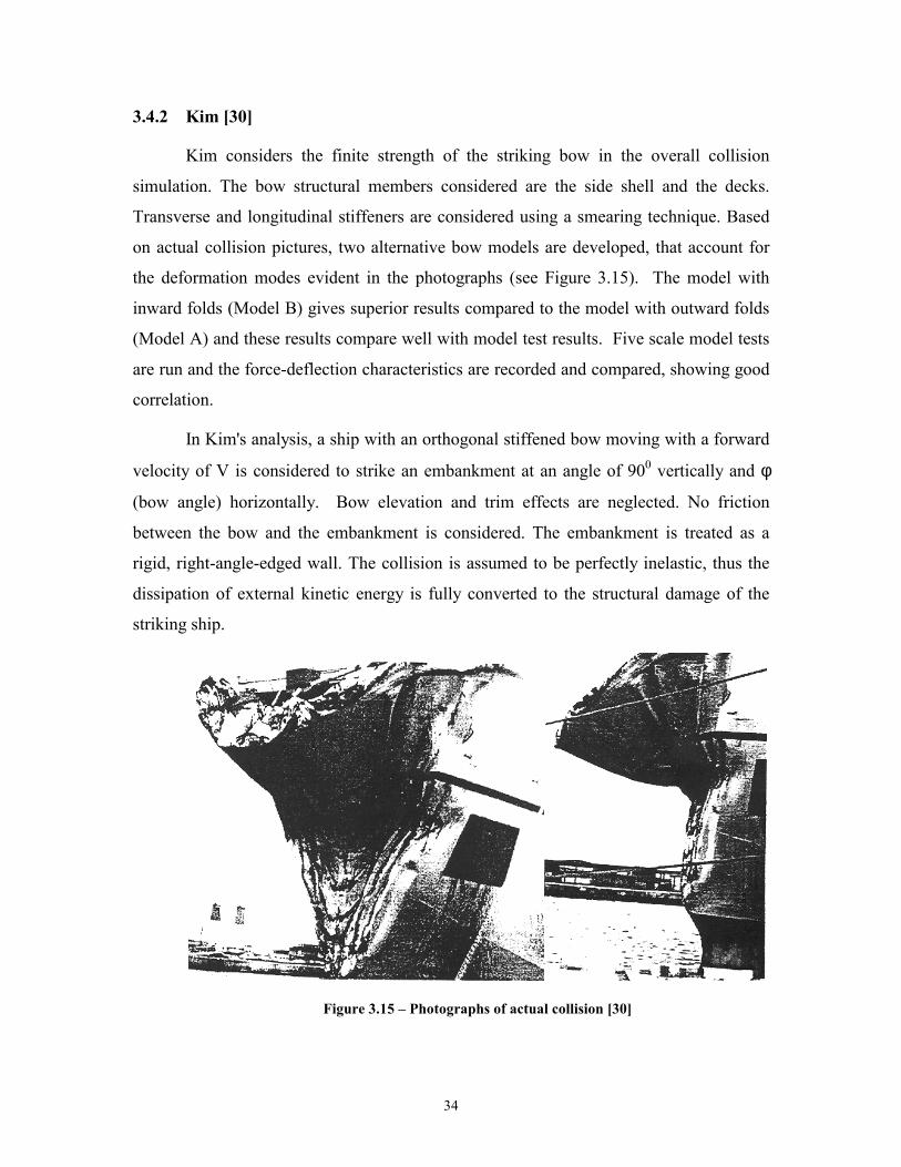
34
3.4.2 Kim [30]
Kim considers the finite strength of the striking bow in the overall collision
simulation. The bow structural members considered are the side shell and the decks.
Transverse and longitudinal stiffeners are considered using a smearing technique. Based
on actual collision pictures, two alternative bow models are developed, that account for
the deformation modes evident in the photographs (see Figure 3.15). The model with
inward folds (Model B) gives superior results compared to the model with outward folds
(Model A) and these results compare well with model test results. Five scale model tests
are run and the force-deflection characteristics are recorded and compared, showing good
correlation.
In Kim's analysis, a ship with an orthogonal stiffened bow moving with a forward
velocity of V is considered to strike an embankment at an angle of 900 vertically and φ
(bow angle) horizontally. Bow elevation and trim effects are neglected. No friction
between the bow and the embankment is considered. The embankment is treated as a
rigid, right-angle-edged wall. The collision is assumed to be perfectly inelastic, thus the
dissipation of external kinetic energy is fully converted to the structural damage of the
striking ship.
Figure 3.15 – Photographs of actual collision [30]
35
Since the bow has complex three-dimensional geometry, it is necessary to
simplify the bow geometry. First, the contact point between the ship and the rigid
obstacle is specified. It is observed from actual accidents and tests that the contact point
divides the bow length in two parts with same length and the vertical extension of the line
from the end of the bow length to the deck plate gives the boundary of the deforming part
of the bow. The bow model in this study is defined using three independent variables,
bow length (l), bow angle (φ) and deck angle (θ). All edge lines in the bow are then
defined in terms of these 3 parameters.
Photographs of the actual collision shown in Figure3.15 show quite a complex
deformation mode. However, by careful inspection, it is observed that there are four
major internal energy dissipation areas, which are side shell folding, deck tilting, frontal
bow stretching and side shell stretching. It is also noticed that one fold of the side shell of
the bow matches one bend on the deck and the large stretching area from the contact
point and small stretching area on the sides.
The mean crushing forces for models A and B respectively are [30]:
Model A:
ϕϕϕπϕϕϕϕϕφ
TanCosMHlSinMCoslSinNCosHSinN
lHNPm 00
20
20
2
0 44)(8sin
18 ++++= (3.13)
Model B:
)28.6134.0( 20 tltPm +=σ (3.14)
Where:
Pm is the mean crushing force;
N0 is the fully plastic membrane force per unit length;
ϕ= is the bow angle (assumed to be 60 degree);
θ= is the approximate side angle between forefront and collision bulkhead (assumed
to be 30 degree);
l is the distance from the bow tip to the point of application of the load;
t is the bow shell plate thickness (0.21mm and 1.2mm are the two values used in
this study);
H is the folding length;
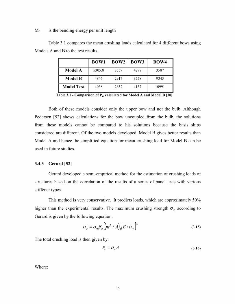
36
M0 is the bending energy per unit length
Table 3.1 compares the mean crushing loads calculated for 4 different bows using
Models A and B to the test results.
BOW1 BOW2 BOW3 BOW4
Model A 5305.8 3557 4278 3587
Model B 4846 2917 3558 9343
Model Test 4038 2652 4137 10991
Table 3.1 - Comparison of Pm calculated for Model A and Model B [30]
Both of these models consider only the upper bow and not the bulb. Although
Pedersen [52] shows calculations for the bow uncoupled from the bulb, the solutions
from these models cannot be compared to his solutions because the basis ships
considered are different. Of the two models developed, Model B gives better results than
Model A and hence the simplified equation for mean crushing load for Model B can be
used in future studies.
3.4.3 Gerard [52]
Gerard developed a semi-empirical method for the estimation of crushing loads of
structures based on the correlation of the results of a series of panel tests with various
stiffener types.
This method is very conservative. It predicts loads, which are approximately 50%
higher than the experimental results. The maximum crushing strength σc, according to
Gerard is given by the following equation:
( )[ ]mygc EAnt σβσσ //20= (3.15)
The total crushing load is then given by:
AP cc σ= (3.16)
Where:
37
σy is the yield stress; σ0 is the compressive flow stress (inclusive strain rate effects); E is the Young’s Modulus for steel; βg=0.56, m=0.85 coefficients depending on edge restraint. The values applied are for
undistorted edges n sum of cuts and flanges for the cross-section under consideration
(See Figure 3.16) t average thickness for the cross-section under consideration; A cross-sectional area
The strain rate is taken as:
ε•= v sx / (3.17)
Where:
νx is the velocity in longitudinal direction during impact; s frame spacing
The magnitude of the dynamic flow stress is calculated from the following relationship:
( ) 037.000 29.1 εσεσ ��
s= (3.18)
where σ0s is the static ultimate strength of the steel material.
The load formula given above predicts the maximum crushing load of plated
structures within ± 10% of the experimental results. One of the major drawbacks of the
model is that it has been derived from the crushing of fairly simple and regular plate
constructions where the range of plating to stiffener thickness ratios and stiffener spacing
are limited. Normal bow structures consist of a number of plate panels of different
dimensions and stiffener sizes.
3.4.4 Amdahl [5, 6]
Amdahl developed a model using intersection elements, correlated against model
test results. Amdahl's method is a modified Wierzbicki [68] method, based on the energy
dissipated during plastic deformation of basic structural elements such as angles, T-
sections and cruciforms (see Figure 3.16). The total crushing load of a specific structure
is obtained by adding up all the basic elements' crushing loads. Amdahl's method predicts
values that are non-conservative, unlike Gerard's method.

38
Amdahl’s procedure leads to the following equation for the average crushing
strength:
67.025.02
67.020 ])
)31.0((31.027.187.0[]/[42.2
tnnA
nnnAtn
TcAT
TcATc +
++= σσ (3.19)
The total crushing load is found by multiplying σc by the associated cross-sectional area
of the deformed steel material:
Pc = σc A (3.20)
Where:
σc is the average crushing strength of the bow;
σ0 is the ultimate strength of steel (incl. strain rate effects);
t is the average thickness of the cross-section under consideration;
A is the cross-sectional area of the deformed steel material;
nc is the number of cruciforms in the cross-section (See Figure 3.16);
nT is the number of T-sections in the cross-section (See Figure 3.16);
nAT is the number of angle- and T-sections in the cross-section (See Figure 3.16)
Figure 3.16 – Method of cross-sections to determine the number of intersections [52]
3.4.5 Yang and Caldwell [70]

39
In Yang and Caldwell, the bow section is modeled as an assembly of basic
elements as shown in Figure 3.16. The mean crushing strength is obtained by summing
the energy dissipated in all individual structural elements.
Figure 3.17 and Figure 3.18 show the different folding mechanisms of the basic
elements and their plane descriptions. The following equations specify the energy
absorbed in the various mechanisms:
• = Mechanism a) cME 01 π= rHMIE
202
24= t
rHMIE 033
16=
1478.12 =I 5779.03 =I (3.21)
Where:
E1 is the energy absorbed due to bending about horizontal hinge lines;
M0 is the corresponding bending moment;
c is the side length of the cross-section of the angle element;
E2 is the energy absorbed by rolling about the moving hinge lines;
E3 is the energy absorbed due to inverting of curvature at the junction;
H is the half-folding length;
r is the radius of the toroidal shell element;
I2 and I3 depend on the joint angle of the basic element;
t is the plate thickness
• = Mechanism b) tHE 24 σ= HME 05 4= (3.22)
Where:
E4 is the energy absorbed during extensional distortion of one plate flange;
E5 is the plastic work in the stationary line at the joint
• = Mechanism c) tHE
206 2σ= HME 07 π= (3.23)
Where:
E6 is the energy absorbed during extensional distortion in the flange after
neglecting shear;
E7 is the plastic work in the stationary line at the joint after neglecting shear
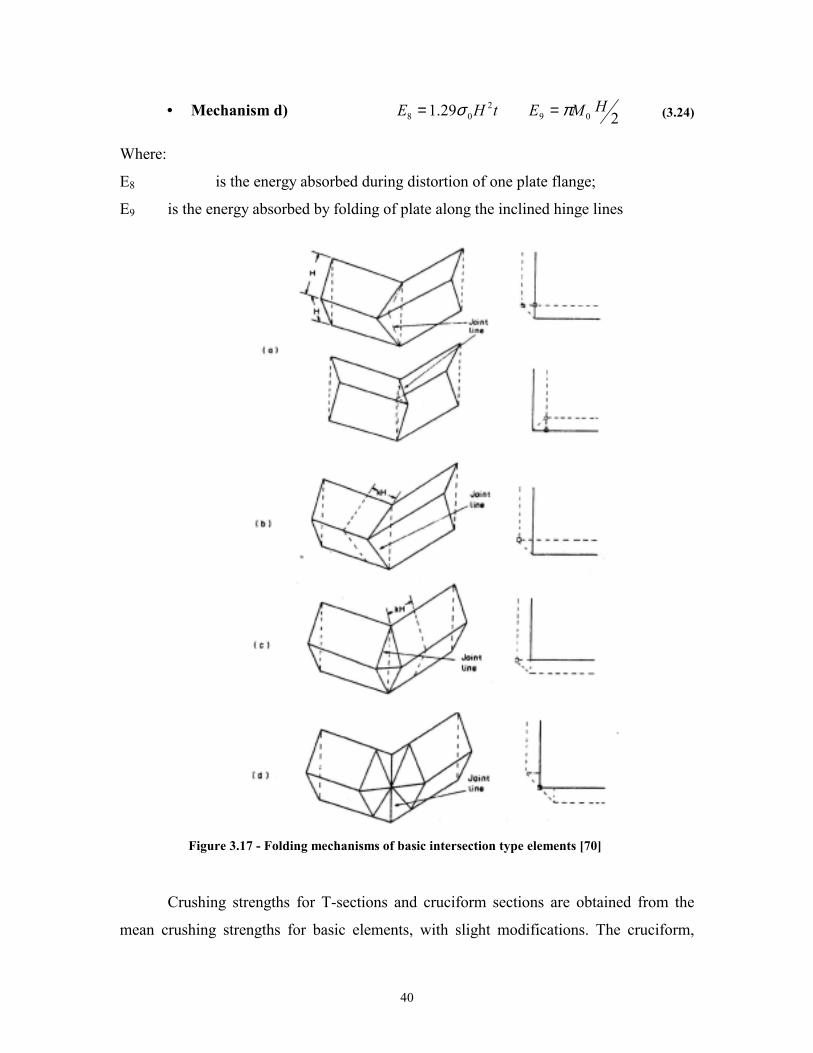
40
• = Mechanism d) tHE 208 29.1 σ= 209
HME π= (3.24)
Where:
E8 is the energy absorbed during distortion of one plate flange;
E9 is the energy absorbed by folding of plate along the inclined hinge lines
Figure 3.17 - Folding mechanisms of basic intersection type elements [70]
Crushing strengths for T-sections and cruciform sections are obtained from the
mean crushing strengths for basic elements, with slight modifications. The cruciform,
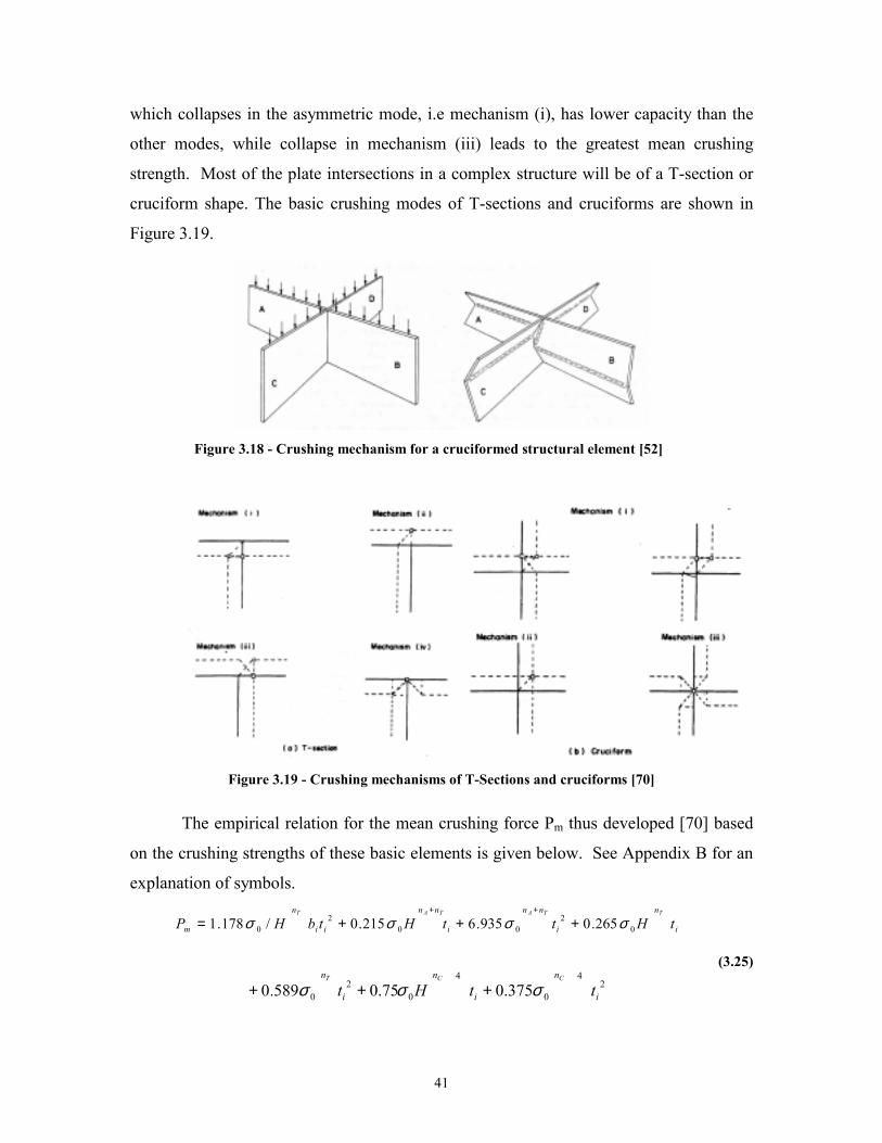
41
which collapses in the asymmetric mode, i.e mechanism (i), has lower capacity than the
other modes, while collapse in mechanism (iii) leads to the greatest mean crushing
strength. Most of the plate intersections in a complex structure will be of a T-section or
cruciform shape. The basic crushing modes of T-sections and cruciforms are shown in
Figure 3.19.
Figure 3.18 - Crushing mechanism for a cruciformed structural element [52]
Figure 3.19 - Crushing mechanisms of T-Sections and cruciforms [70]
The empirical relation for the mean crushing force Pm thus developed [70] based
on the crushing strengths of these basic elements is given below. See Appendix B for an
explanation of symbols. ++
+++=TA TTAT nn n
ii
nn
ii
n
im tHttHtbHP 02
002
0 265.0935.6215.0/178.1 σσσσ
+++CCT n
i
n
i
n
i ttHt4
20
4
02
0 375.075.0589.0 σσσ
(3.25)
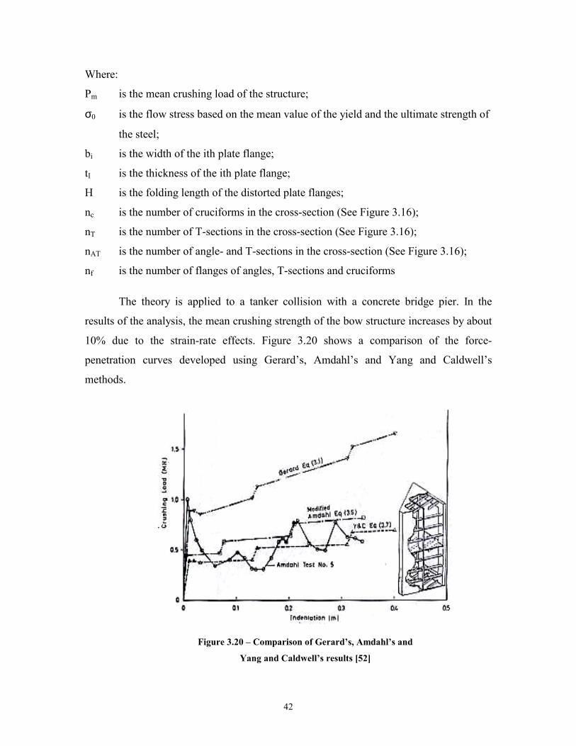
42
Where:
Pm is the mean crushing load of the structure;
σ0 is the flow stress based on the mean value of the yield and the ultimate strength of
the steel;
bi is the width of the ith plate flange;
tI is the thickness of the ith plate flange;
H is the folding length of the distorted plate flanges;
nc is the number of cruciforms in the cross-section (See Figure 3.16);
nT is the number of T-sections in the cross-section (See Figure 3.16);
nAT is the number of angle- and T-sections in the cross-section (See Figure 3.16);
nf is the number of flanges of angles, T-sections and cruciforms
The theory is applied to a tanker collision with a concrete bridge pier. In the
results of the analysis, the mean crushing strength of the bow structure increases by about
10% due to the strain-rate effects. Figure 3.20 shows a comparison of the force-
penetration curves developed using Gerard’s, Amdahl’s and Yang and Caldwell’s
methods.
Figure 3.20 – Comparison of Gerard’s, Amdahl’s and
Yang and Caldwell’s results [52]
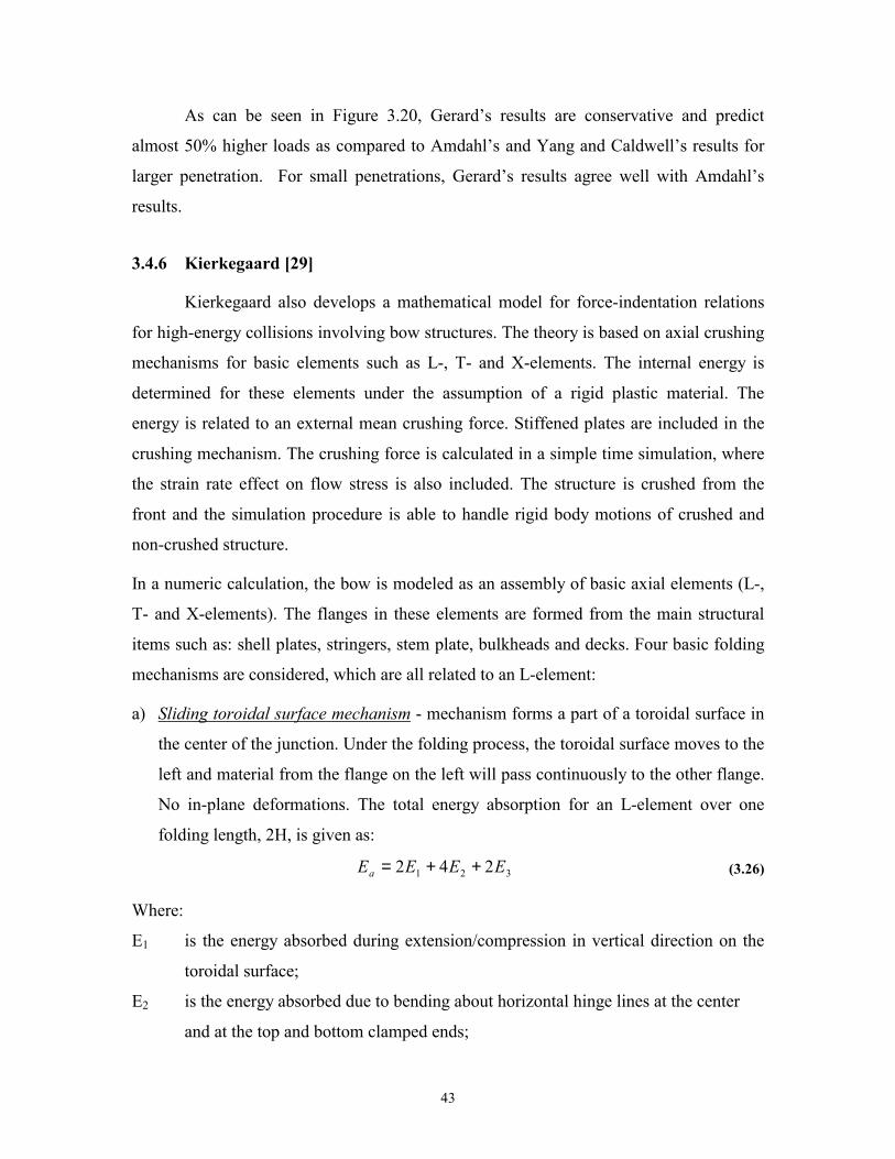
43
As can be seen in Figure 3.20, Gerard’s results are conservative and predict
almost 50% higher loads as compared to Amdahl’s and Yang and Caldwell’s results for
larger penetration. For small penetrations, Gerard’s results agree well with Amdahl’s
results.
3.4.6 Kierkegaard [29]
Kierkegaard also develops a mathematical model for force-indentation relations
for high-energy collisions involving bow structures. The theory is based on axial crushing
mechanisms for basic elements such as L-, T- and X-elements. The internal energy is
determined for these elements under the assumption of a rigid plastic material. The
energy is related to an external mean crushing force. Stiffened plates are included in the
crushing mechanism. The crushing force is calculated in a simple time simulation, where
the strain rate effect on flow stress is also included. The structure is crushed from the
front and the simulation procedure is able to handle rigid body motions of crushed and
non-crushed structure.
In a numeric calculation, the bow is modeled as an assembly of basic axial elements (L-,
T- and X-elements). The flanges in these elements are formed from the main structural
items such as: shell plates, stringers, stem plate, bulkheads and decks. Four basic folding
mechanisms are considered, which are all related to an L-element:
a) Sliding toroidal surface mechanism - mechanism forms a part of a toroidal surface in
the center of the junction. Under the folding process, the toroidal surface moves to the
left and material from the flange on the left will pass continuously to the other flange.
No in-plane deformations. The total energy absorption for an L-element over one
folding length, 2H, is given as:
321 242 EEEEa ++= (3.26)
Where:
E1 is the energy absorbed during extension/compression in vertical direction on the
toroidal surface;
E2 is the energy absorbed due to bending about horizontal hinge lines at the center
and at the top and bottom clamped ends;

44
E2 is the energy absorbed due to bending about vertical moving hinge lines
b) One flange extension mechanism - The intersection line breaks to the side without any
material transfer across the intersection. The energy in this case is:
5424 EEEEb ++= (3.27)
Where E4 is the energy from extension and E5 is the energy from bending.
c) Straight edge mechanism - Under the folding process, the intersection line between
the flanges will remain straight and vertical. Then the triangular sections with a side
coinciding with the intersection line will be compressed in-plane in the x-direction
and the other triangular plate sections will be transformed by shear and extension in
the horizontal direction. The energy absorbed in this case is:
762 224 EEEEc ++= (3.28)
Where E6 and E7 are the energies dissipated in bending along the vertical hinge lines.
d) In-plane deformation mechanism - Energy is absorbed through shape distortion of
each of the four rectangular sections. These plane deformations are dominated by
extension/compression in the y-direction. Also, a minor part is absorbed in bending
about the joint-line. The energy absorbed here is:
E E E Ed= + +4 2 22 8 9 (3.29)
Where E8 and E9 are the energies dissipated in one flange during extension and bending
in the joint line.
The mean crushing force can then be found as:
P Em
i
e
=∂
(3.30)
Where EI is the energy absorption over one folding length 2H and
∂ =e H23
2 (3.31)
The mean crushing force for the four mechanisms is shown in the Figure 3.21.
Crushing mechanisms for T- and X-elements can be generated from the four basic
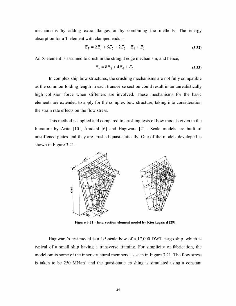
45
mechanisms by adding extra flanges or by combining the methods. The energy
absorption for a T-element with clamped ends is:
(3.32)
An X-element is assumed to crush in the straight edge mechanism, and hence,
(3.33)
In complex ship bow structures, the crushing mechanisms are not fully compatible
as the common folding length in each transverse section could result in an unrealistically
high collision force when stiffeners are involved. These mechanisms for the basic
elements are extended to apply for the complex bow structure, taking into consideration
the strain rate effects on the flow stress.
This method is applied and compared to crushing tests of bow models given in the
literature by Arita [10], Amdahl [6] and Hagiwara [21]. Scale models are built of
unstiffened plates and they are crushed quasi-statically. One of the models developed is
shown in Figure 3.21.
Figure 3.21 - Intersection element model by Kierkegaard [29]
Hagiwara’s test model is a 1/5-scale bow of a 17,000 DWT cargo ship, which is
typical of a small ship having a transverse framing. For simplicity of fabrication, the
model omits some of the inner structural members, as seen in Figure 3.21. The flow stress
is taken to be 250 MN/m2 and the quasi-static crushing is simulated using a constant
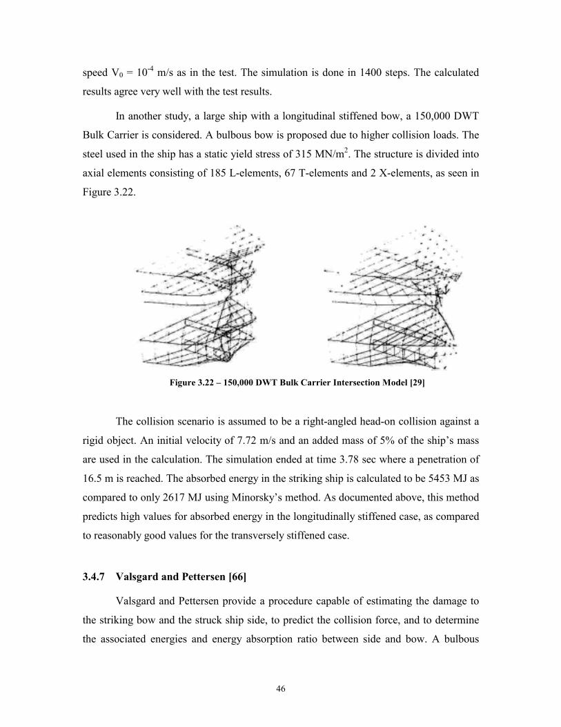
46
speed V0 = 10-4 m/s as in the test. The simulation is done in 1400 steps. The calculated
results agree very well with the test results.
In another study, a large ship with a longitudinal stiffened bow, a 150,000 DWT
Bulk Carrier is considered. A bulbous bow is proposed due to higher collision loads. The
steel used in the ship has a static yield stress of 315 MN/m2. The structure is divided into
axial elements consisting of 185 L-elements, 67 T-elements and 2 X-elements, as seen in
Figure 3.22.
Figure 3.22 – 150,000 DWT Bulk Carrier Intersection Model [29]
The collision scenario is assumed to be a right-angled head-on collision against a
rigid object. An initial velocity of 7.72 m/s and an added mass of 5% of the ship’s mass
are used in the calculation. The simulation ended at time 3.78 sec where a penetration of
16.5 m is reached. The absorbed energy in the striking ship is calculated to be 5453 MJ as
compared to only 2617 MJ using Minorsky’s method. As documented above, this method
predicts high values for absorbed energy in the longitudinally stiffened case, as compared
to reasonably good values for the transversely stiffened case.
3.4.7 Valsgard and Pettersen [66]
Valsgard and Pettersen provide a procedure capable of estimating the damage to
the striking bow and the struck ship side, to predict the collision force, and to determine
the associated energies and energy absorption ratio between side and bow. A bulbous
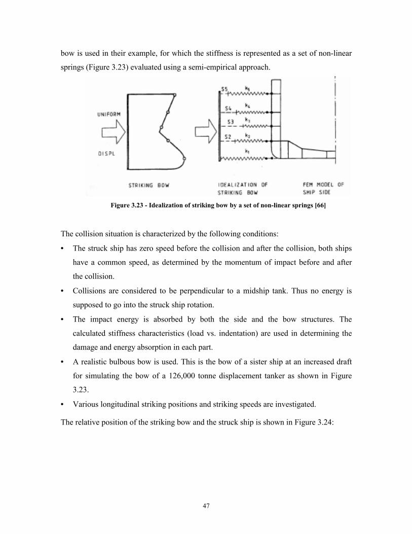
47
bow is used in their example, for which the stiffness is represented as a set of non-linear
springs (Figure 3.23) evaluated using a semi-empirical approach.
Figure 3.23 - Idealization of striking bow by a set of non-linear springs [66]
The collision situation is characterized by the following conditions:
• = The struck ship has zero speed before the collision and after the collision, both ships
have a common speed, as determined by the momentum of impact before and after
the collision.
• = Collisions are considered to be perpendicular to a midship tank. Thus no energy is
supposed to go into the struck ship rotation.
• = The impact energy is absorbed by both the side and the bow structures. The
calculated stiffness characteristics (load vs. indentation) are used in determining the
damage and energy absorption in each part.
• = A realistic bulbous bow is used. This is the bow of a sister ship at an increased draft
for simulating the bow of a 126,000 tonne displacement tanker as shown in Figure
3.23.
• = Various longitudinal striking positions and striking speeds are investigated.
The relative position of the striking bow and the struck ship is shown in Figure 3.24:
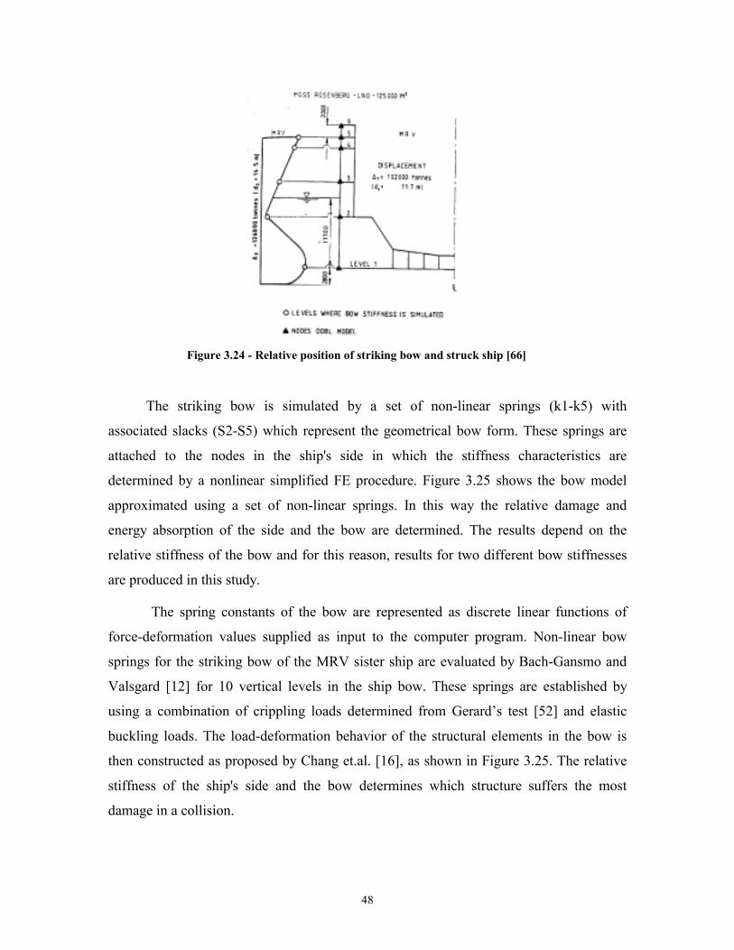
48
Figure 3.24 - Relative position of striking bow and struck ship [66]
The striking bow is simulated by a set of non-linear springs (k1-k5) with
associated slacks (S2-S5) which represent the geometrical bow form. These springs are
attached to the nodes in the ship's side in which the stiffness characteristics are
determined by a nonlinear simplified FE procedure. Figure 3.25 shows the bow model
approximated using a set of non-linear springs. In this way the relative damage and
energy absorption of the side and the bow are determined. The results depend on the
relative stiffness of the bow and for this reason, results for two different bow stiffnesses
are produced in this study.
The spring constants of the bow are represented as discrete linear functions of
force-deformation values supplied as input to the computer program. Non-linear bow
springs for the striking bow of the MRV sister ship are evaluated by Bach-Gansmo and
Valsgard [12] for 10 vertical levels in the ship bow. These springs are established by
using a combination of crippling loads determined from Gerard’s test [52] and elastic
buckling loads. The load-deformation behavior of the structural elements in the bow is
then constructed as proposed by Chang et.al. [16], as shown in Figure 3.25. The relative
stiffness of the ship's side and the bow determines which structure suffers the most
damage in a collision.
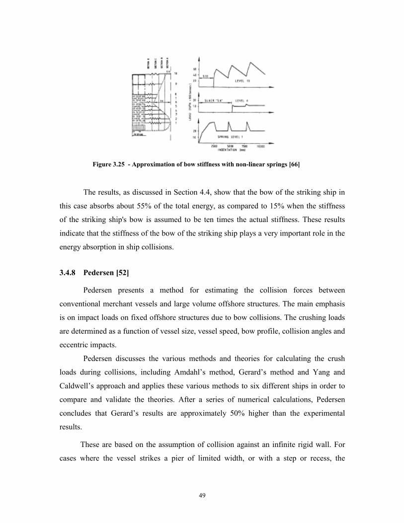
49
Figure 3.25 - Approximation of bow stiffness with non-linear springs [66]
The results, as discussed in Section 4.4, show that the bow of the striking ship in
this case absorbs about 55% of the total energy, as compared to 15% when the stiffness
of the striking ship's bow is assumed to be ten times the actual stiffness. These results
indicate that the stiffness of the bow of the striking ship plays a very important role in the
energy absorption in ship collisions.
3.4.8 Pedersen [52]
Pedersen presents a method for estimating the collision forces between
conventional merchant vessels and large volume offshore structures. The main emphasis
is on impact loads on fixed offshore structures due to bow collisions. The crushing loads
are determined as a function of vessel size, vessel speed, bow profile, collision angles and
eccentric impacts.
Pedersen discusses the various methods and theories for calculating the crush
loads during collisions, including Amdahl’s method, Gerard’s method and Yang and
Caldwell’s approach and applies these various methods to six different ships in order to
compare and validate the theories. After a series of numerical calculations, Pedersen
concludes that Gerard’s results are approximately 50% higher than the experimental
results.
These are based on the assumption of collision against an infinite rigid wall. For
cases where the vessel strikes a pier of limited width, or with a step or recess, the
50
collision force needs to be adjusted by multiplying the ratio of the deformed steel area in
actual contact with the pier to the total steel area of the bow section under consideration.
In addition, shear forces are to be included as shown in the equation below:
+=dn
FRdcrcccl StAAPP τ/ (3.34)
Where:
Pcl is the collision load on the pier based on contact area assessment;
Pc is the collision load on plane infinite wall;
Ac is the cross-sectional area of the steel material in direct contact with the pier
during deformation of bow;
A is the total cross-sectional area of the steel material at the section of the bow
under consideration;
nd is the number of decks and sides extending outside the pier width;
τcr is the shear buckling stress of decks and sides extending outside the pier
Six different ships are considered: 1) 150,000 DWT Bulk Carrier, 2) 40,000 DWT
containership, 3) 3000 DWT general cargo vessel, 4) 2000 DWT tanker, 5) 1000 DWT
pallet carrier 6) 500 DWT coaster. All these ships have bulbs. The main particulars and
the bow scantlings of these ships are given in Appendix C.
Figure 3.26 shows the calculated crushing load-indentation curves using
Amdahl’s modified method and Yang and Caldwell’s method for the 150,000 DWT bulk
vessel in a fully loaded condition, striking head-on with a rigid wall at an initial impact
speed of 18 knots. Similar results for the 40,000 DWT container vessel for a head-on
collision with a rigid wall at an initial speed of 12.9 m/s are obtained.
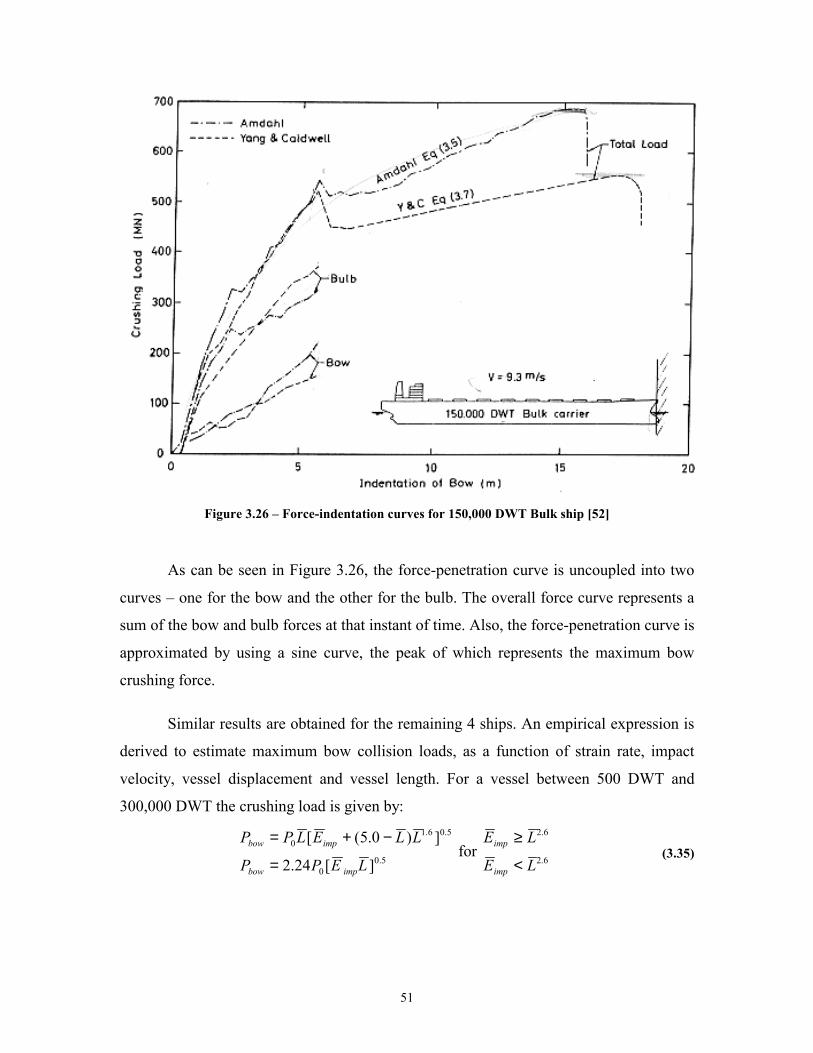
51
Figure 3.26 – Force-indentation curves for 150,000 DWT Bulk ship [52]
As can be seen in Figure 3.26, the force-penetration curve is uncoupled into two
curves – one for the bow and the other for the bulb. The overall force curve represents a
sum of the bow and bulb forces at that instant of time. Also, the force-penetration curve is
approximated by using a sine curve, the peak of which represents the maximum bow
crushing force.
Similar results are obtained for the remaining 4 ships. An empirical expression is
derived to estimate maximum bow collision loads, as a function of strain rate, impact
velocity, vessel displacement and vessel length. For a vessel between 500 DWT and
300,000 DWT the crushing load is given by:
5.00
5.06.10
][24.2
])0.5([
LEPP
LLELPP
impbow
impbow
=
−+= for
6.2
6.2
LE
LE
imp
imp
<
≥ (3.35)
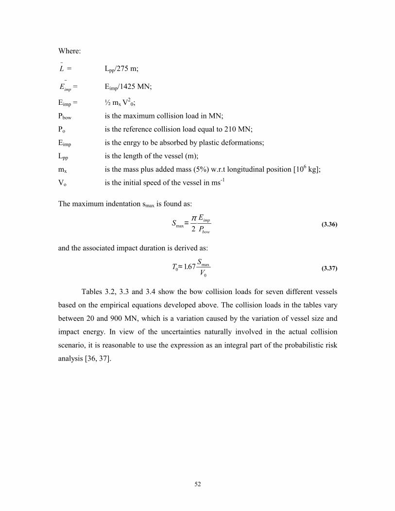
52
Where:
L−
= Lpp/275 m;
Eimp
−= Eimp/1425 MN;
Eimp = ½ mx V20;
Pbow is the maximum collision load in MN;
Po is the reference collision load equal to 210 MN;
Eimp is the enrgy to be absorbed by plastic deformations;
Lpp is the length of the vessel (m);
mx is the mass plus added mass (5%) w.r.t longitudinal position [106 kg];
Vo is the initial speed of the vessel in ms-1
The maximum indentation smax is found as:
SEP
imp
bowmax=
π2
(3.36)
and the associated impact duration is derived as:
T SV0
0
167≈ . max (3.37)
Tables 3.2, 3.3 and 3.4 show the bow collision loads for seven different vessels
based on the empirical equations developed above. The collision loads in the tables vary
between 20 and 900 MN, which is a variation caused by the variation of vessel size and
impact energy. In view of the uncertainties naturally involved in the actual collision
scenario, it is reasonable to use the expression as an integral part of the probabilistic risk
analysis [36, 37].
53
Table 3.2 – F, d and t for five fully loaded ships [52]
Table 3.3 –F, d and t for a bulk carrier at various speeds [52]
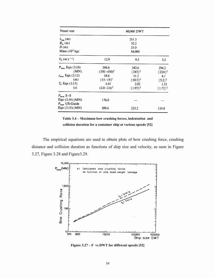
54
Table 3.4 – Maximum bow crushing forces, indentation and
collision duration for a container ship at various speeds [52]
The empirical equations are used to obtain plots of bow crushing force, crushing
distance and collision duration as functions of ship size and velocity, as seen in Figure
3.27, Figure 3.28 and Figure3.29.
Figure 3.27 – F vs DWT for different speeds [52]
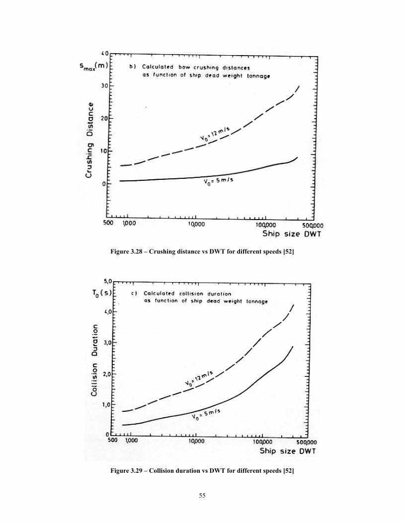
55
Figure 3.28 – Crushing distance vs DWT for different speeds [52]
Figure 3.29 – Collision duration vs DWT for different speeds [52]

56
3.5 Comparison of the models
Table 3.1 below summarizes the various bow models described in the
sections above and reviews the salient points to be remembered from each of these
models.
Model R
igid
Def
orm
able
Clo
sed-
Form
Equ
atio
n
FE-B
ased
Empi
rica
l
Inte
rsec
tion
Elem
ents
Bow
Infin
ite W
edge
Num
eric
al E
xam
ples
Rel
ativ
e D
raft
Uun
coup
led
Bulb
, Bow
Minorsky [40]
Hutchison [25]
Ito [27]
Wierzbicki [68]
Simonsen [62]
SIMCOL 0.1 – 2.0 [17]
SIMCOL 2.1 [17]
Woisin [69]
Kim [20]
Gerard [52]
Amdahl [52]
Kierkegaard [29]
Yang and Caldwell [70]
Pedersen [52]
Valsgard, Pettersen [66]
Table 3.5 – Comparison of important features of various bow models
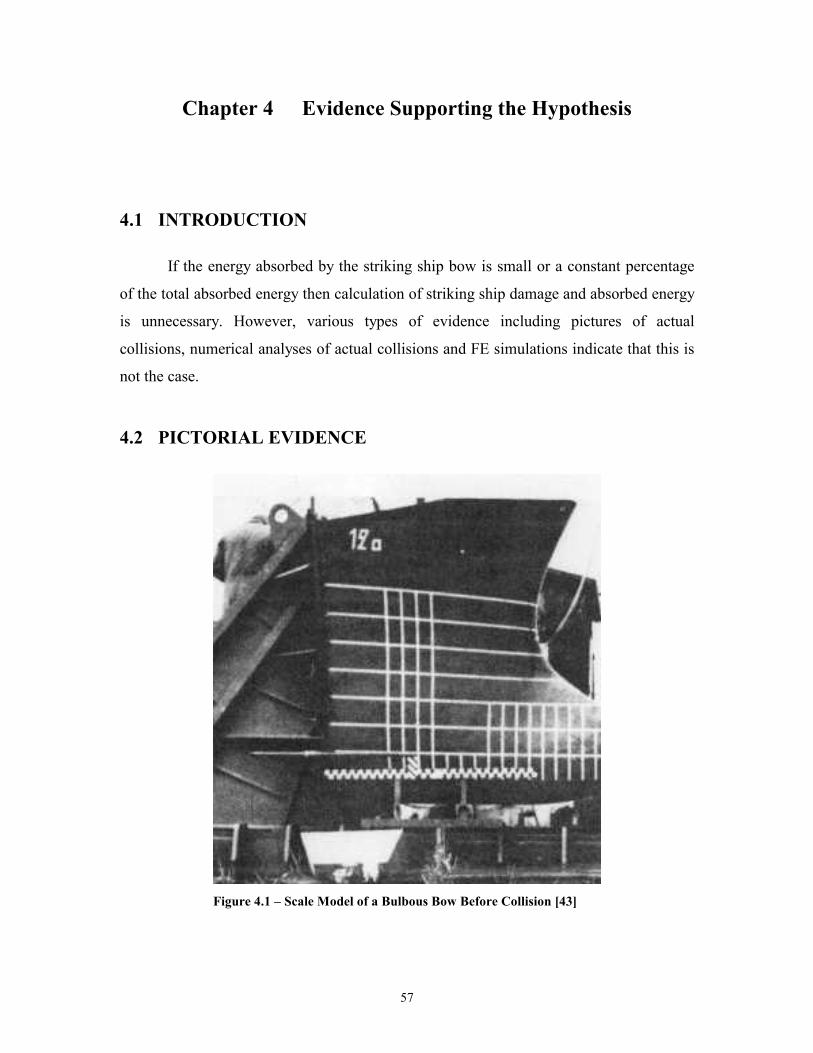
57
Chapter 4 Evidence Supporting the Hypothesis 4.1 INTRODUCTION
If the energy absorbed by the striking ship bow is small or a constant percentage
of the total absorbed energy then calculation of striking ship damage and absorbed energy
is unnecessary. However, various types of evidence including pictures of actual
collisions, numerical analyses of actual collisions and FE simulations indicate that this is
not the case.
4.2 PICTORIAL EVIDENCE
Figure 4.1 – Scale Model of a Bulbous Bow Before Collision [43]
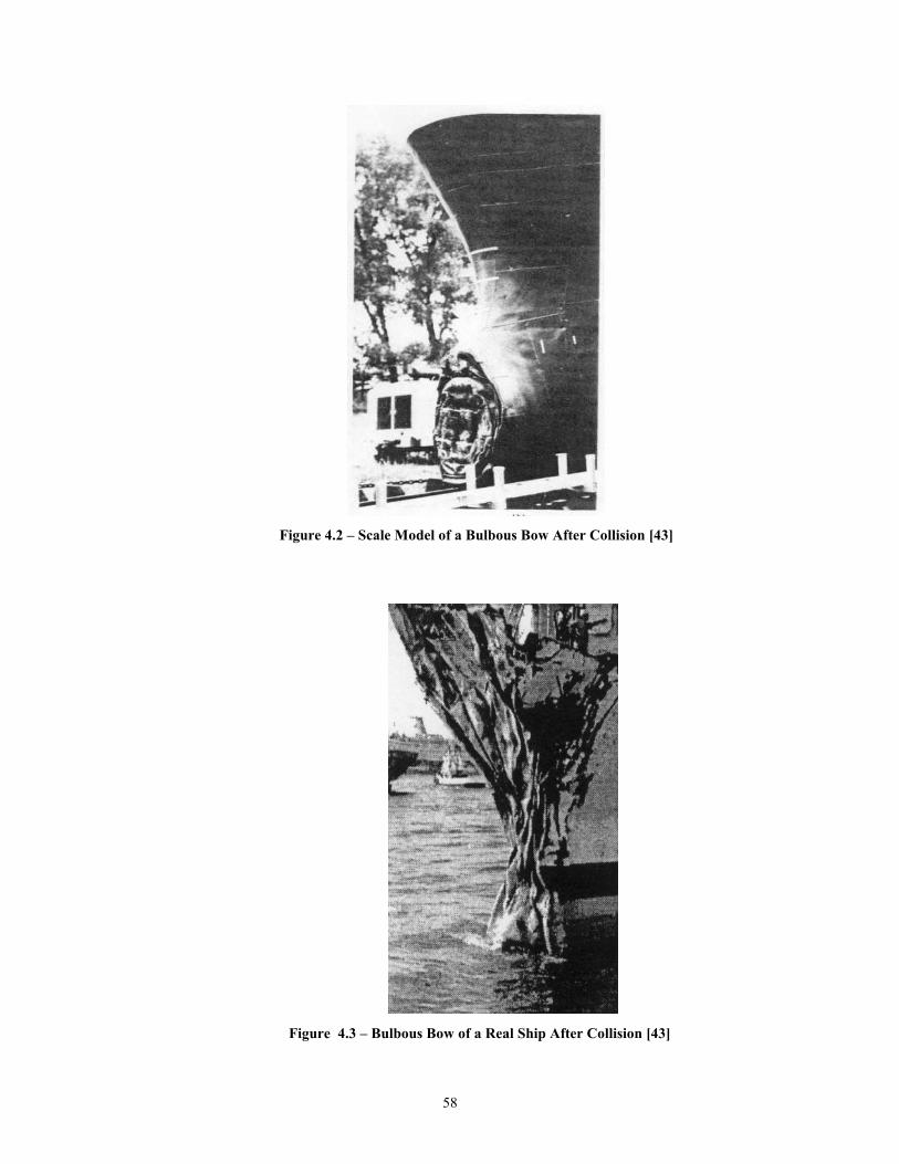
58
Figure 4.2 – Scale Model of a Bulbous Bow After Collision [43]
Figure 4.3 – Bulbous Bow of a Real Ship After Collision [43]
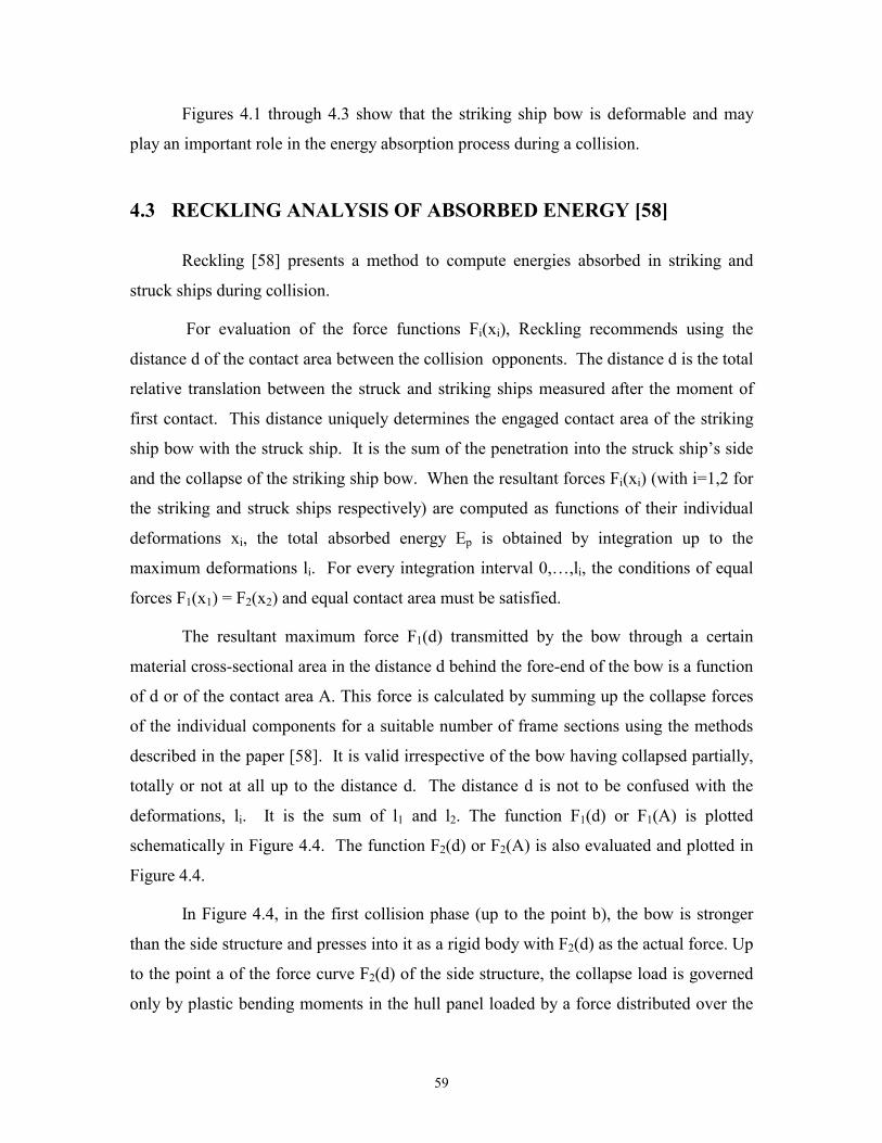
59
Figures 4.1 through 4.3 show that the striking ship bow is deformable and may
play an important role in the energy absorption process during a collision.
4.3 RECKLING ANALYSIS OF ABSORBED ENERGY [58]
Reckling [58] presents a method to compute energies absorbed in striking and
struck ships during collision.
For evaluation of the force functions Fi(xi), Reckling recommends using the
distance d of the contact area between the collision opponents. The distance d is the total
relative translation between the struck and striking ships measured after the moment of
first contact. This distance uniquely determines the engaged contact area of the striking
ship bow with the struck ship. It is the sum of the penetration into the struck ship’s side
and the collapse of the striking ship bow. When the resultant forces Fi(xi) (with i=1,2 for
the striking and struck ships respectively) are computed as functions of their individual
deformations xi, the total absorbed energy Ep is obtained by integration up to the
maximum deformations li. For every integration interval 0,…,li, the conditions of equal
forces F1(x1) = F2(x2) and equal contact area must be satisfied.
The resultant maximum force F1(d) transmitted by the bow through a certain
material cross-sectional area in the distance d behind the fore-end of the bow is a function
of d or of the contact area A. This force is calculated by summing up the collapse forces
of the individual components for a suitable number of frame sections using the methods
described in the paper [58]. It is valid irrespective of the bow having collapsed partially,
totally or not at all up to the distance d. The distance d is not to be confused with the
deformations, li. It is the sum of l1 and l2. The function F1(d) or F1(A) is plotted
schematically in Figure 4.4. The function F2(d) or F2(A) is also evaluated and plotted in
Figure 4.4.
In Figure 4.4, in the first collision phase (up to the point b), the bow is stronger
than the side structure and presses into it as a rigid body with F2(d) as the actual force. Up
to the point a of the force curve F2(d) of the side structure, the collapse load is governed
only by plastic bending moments in the hull panel loaded by a force distributed over the
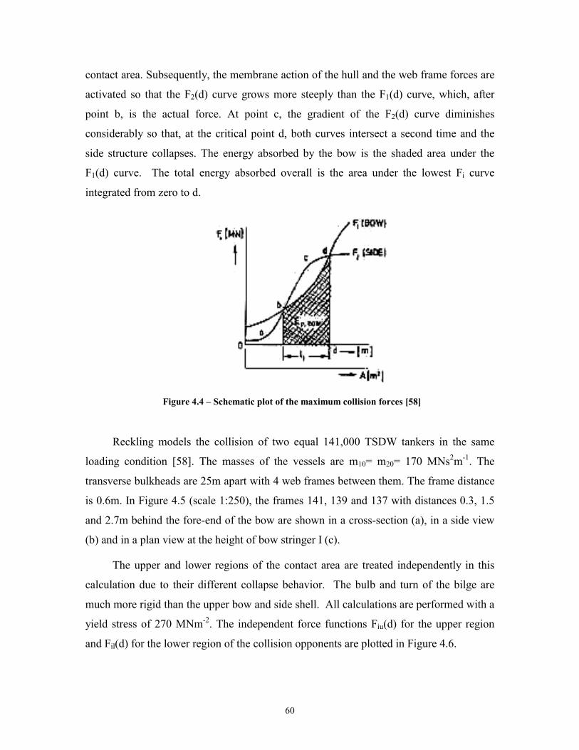
60
contact area. Subsequently, the membrane action of the hull and the web frame forces are
activated so that the F2(d) curve grows more steeply than the F1(d) curve, which, after
point b, is the actual force. At point c, the gradient of the F2(d) curve diminishes
considerably so that, at the critical point d, both curves intersect a second time and the
side structure collapses. The energy absorbed by the bow is the shaded area under the
F1(d) curve. The total energy absorbed overall is the area under the lowest Fi curve
integrated from zero to d.
Figure 4.4 – Schematic plot of the maximum collision forces [58]
Reckling models the collision of two equal 141,000 TSDW tankers in the same
loading condition [58]. The masses of the vessels are m10= m20= 170 MNs2m-1. The
transverse bulkheads are 25m apart with 4 web frames between them. The frame distance
is 0.6m. In Figure 4.5 (scale 1:250), the frames 141, 139 and 137 with distances 0.3, 1.5
and 2.7m behind the fore-end of the bow are shown in a cross-section (a), in a side view
(b) and in a plan view at the height of bow stringer I (c).
The upper and lower regions of the contact area are treated independently in this
calculation due to their different collapse behavior. The bulb and turn of the bilge are
much more rigid than the upper bow and side shell. All calculations are performed with a
yield stress of 270 MNm-2. The independent force functions Fiu(d) for the upper region
and Fil(d) for the lower region of the collision opponents are plotted in Figure 4.6.
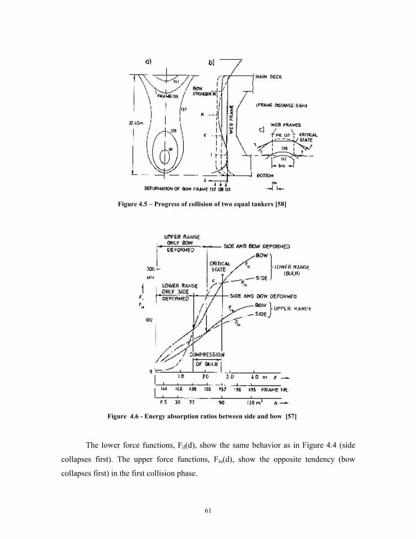
61
Figure 4.5 – Progress of collision of two equal tankers [58]
Figure 4.6 - Energy absorption ratios between side and bow [57]
The lower force functions, Fil(d), show the same behavior as in Figure 4.4 (side
collapses first). The upper force functions, Fiu(d), show the opposite tendency (bow
collapses first) in the first collision phase.
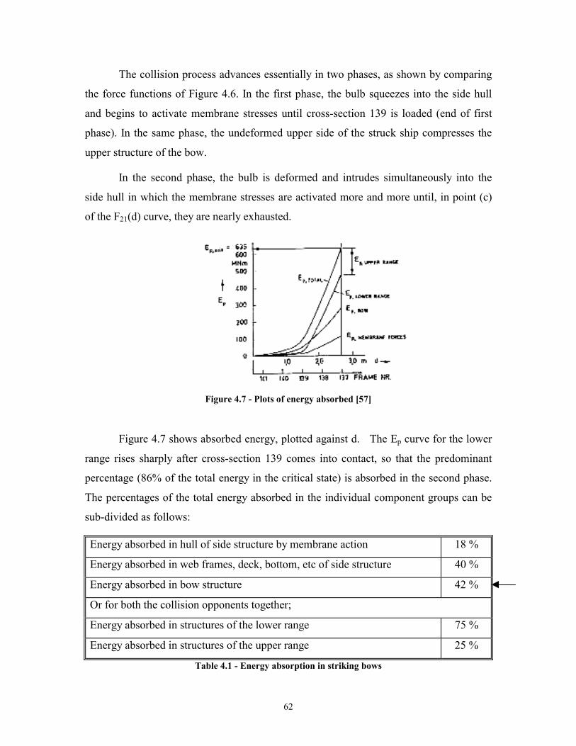
62
The collision process advances essentially in two phases, as shown by comparing
the force functions of Figure 4.6. In the first phase, the bulb squeezes into the side hull
and begins to activate membrane stresses until cross-section 139 is loaded (end of first
phase). In the same phase, the undeformed upper side of the struck ship compresses the
upper structure of the bow.
In the second phase, the bulb is deformed and intrudes simultaneously into the
side hull in which the membrane stresses are activated more and more until, in point (c)
of the F21(d) curve, they are nearly exhausted.
Figure 4.7 - Plots of energy absorbed [57]
Figure 4.7 shows absorbed energy, plotted against d. The Ep curve for the lower
range rises sharply after cross-section 139 comes into contact, so that the predominant
percentage (86% of the total energy in the critical state) is absorbed in the second phase.
The percentages of the total energy absorbed in the individual component groups can be
sub-divided as follows:
Energy absorbed in hull of side structure by membrane action 18 %
Energy absorbed in web frames, deck, bottom, etc of side structure 40 %
Energy absorbed in bow structure 42 %
Or for both the collision opponents together;
Energy absorbed in structures of the lower range 75 %
Energy absorbed in structures of the upper range 25 %
Table 4.1 - Energy absorption in striking bows
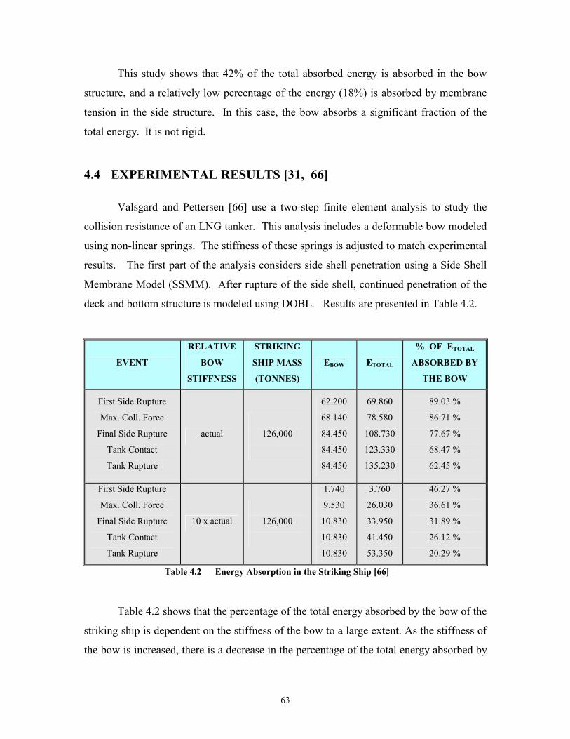
63
This study shows that 42% of the total absorbed energy is absorbed in the bow
structure, and a relatively low percentage of the energy (18%) is absorbed by membrane
tension in the side structure. In this case, the bow absorbs a significant fraction of the
total energy. It is not rigid.
4.4 EXPERIMENTAL RESULTS [31, 66]
Valsgard and Pettersen [66] use a two-step finite element analysis to study the
collision resistance of an LNG tanker. This analysis includes a deformable bow modeled
using non-linear springs. The stiffness of these springs is adjusted to match experimental
results. The first part of the analysis considers side shell penetration using a Side Shell
Membrane Model (SSMM). After rupture of the side shell, continued penetration of the
deck and bottom structure is modeled using DOBL. Results are presented in Table 4.2.
EVENT
RELATIVE
BOW
STIFFNESS
STRIKING
SHIP MASS
(TONNES)
EBOW ETOTAL
% OF ETOTAL
ABSORBED BY
THE BOW
First Side Rupture
Max. Coll. Force
Final Side Rupture
Tank Contact
Tank Rupture
actual
126,000
62.200
68.140
84.450
84.450
84.450
69.860
78.580
108.730
123.330
135.230
89.03 %
86.71 %
77.67 %
68.47 %
62.45 %
First Side Rupture
Max. Coll. Force
Final Side Rupture
Tank Contact
Tank Rupture
10 x actual
126,000
1.740
9.530
10.830
10.830
10.830
3.760
26.030
33.950
41.450
53.350
46.27 %
36.61 %
31.89 %
26.12 %
20.29 %
Table 4.2 Energy Absorption in the Striking Ship [66]
Table 4.2 shows that the percentage of the total energy absorbed by the bow of the
striking ship is dependent on the stiffness of the bow to a large extent. As the stiffness of
the bow is increased, there is a decrease in the percentage of the total energy absorbed by
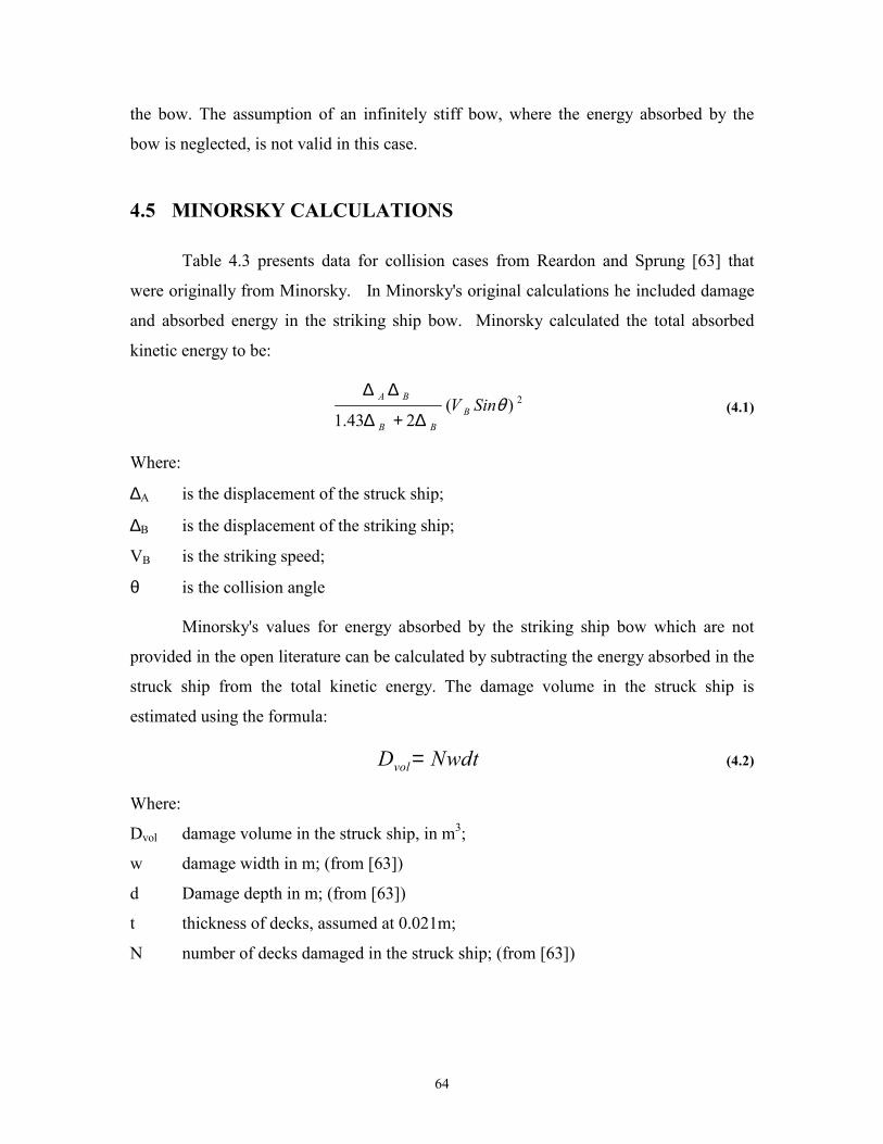
64
the bow. The assumption of an infinitely stiff bow, where the energy absorbed by the
bow is neglected, is not valid in this case.
4.5 MINORSKY CALCULATIONS
Table 4.3 presents data for collision cases from Reardon and Sprung [63] that
were originally from Minorsky. In Minorsky's original calculations he included damage
and absorbed energy in the striking ship bow. Minorsky calculated the total absorbed
kinetic energy to be:
2)(243.1
θSinV BBB
BA
∆+∆
∆∆ (4.1)
Where:
∆A is the displacement of the struck ship;
∆B is the displacement of the striking ship;
VB is the striking speed;
θ is the collision angle
Minorsky's values for energy absorbed by the striking ship bow which are not
provided in the open literature can be calculated by subtracting the energy absorbed in the
struck ship from the total kinetic energy. The damage volume in the struck ship is
estimated using the formula:
D Nwdtvol= (4.2)
Where:
Dvol damage volume in the struck ship, in m3;
w damage width in m; (from [63])
d Damage depth in m; (from [63])
t thickness of decks, assumed at 0.021m;
N number of decks damaged in the struck ship; (from [63])
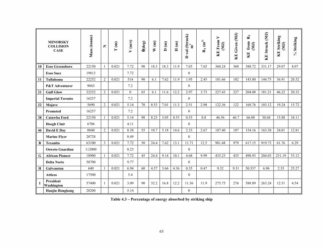
65
MINORSKY COLLISION
CASE
Mas
s (to
nne)
N
T (m
)
V (m
/s)
θθ θθ(de
g)
W (m
)
D (m
)
H (m
)
D v
ol (S
truc
k)
m3
RT (m
3)
KE
From
V
(MJ)
KE
Giv
en (M
J)
KE
from
RT
(MJ)
KE
Stru
ck (M
J)
KE
Stri
king
(M
J)
% S
trik
ing
10 Esso Greensboro 22150 1 0.021 7.72 90 18.3 18.3 11.9 7.03 7.65 360.24 360 388.72 331.17 29.07 8.07
Esso Suez 19813 7.72 0
11 Tullahoma 22252 2 0.021 514 90 6.1 7.62 11.9 1.95 2.45 181.66 182 143.80 144.75 36.91 20.32
P&T Adventurer 9043 7.2 0
21 Gulf Glow 22252 2 0.021 0 65 6.1 11.6 12.2 2.97 3.73 227.43 227 204.08 181.21 46.22 20.32
Imperial Toronto 16257 7.2 0
22 Mojave 5690 2 0.021 5.14 70 8.53 7.01 11.3 2.51 2.98 122.36 122 168.76 103.12 19.24 15.72
Prometed 16257 7.2 0
38 Catawba Ford 22150 1 0.021 5.14 90 8.23 3.05 8.53 0.53 0.8 46.56 46.7 66.08 30.68 15.88 34.11
Hoegh Clair 6706 4.11 0
46 David E Day 8840 2 0.021 8.38 55 10.7 5.18 14.6 2.33 2.67 187.40 187 154.16 163.38 24.01 12.81
Marine Flyer 20728 8.49 0
B Texanita 63100 3 0.021 7.72 50 24.4 7.62 13.1 11.71 12.5 981.48 979 617.15 919.73 61.76 6.29
Osweto Guardian 112000 8.23 0
G African Pioneer 18900 1 0.021 7.72 45 24.4 9.14 10.1 4.68 9.99 435.23 435 498.93 204.03 231.19 53.12
Delta Norte 58700 9.77 0
H Galvenston 640 1 0.021 6.94 60 4.57 3.66 4.36 0.35 0.47 9.32 9.31 50.537 6.96 2.35 25.27
Atticos 17500 5.4 0
I President Washington 57400 1 0.021 3.09 90 32.2 16.8 12.2 11.36 11.9 275.75 276 588.89 263.24 12.51 4.54
Hanjin Hongkong 28200 5.14 0
Table 4.3 – Percentage of energy absorbed by striking ship
66
Energy absorbed by the struck ship is given by:
KE DR
KEstruckvol
Tgiven= (4.3)
The percentage of energy absorbed by the striking ship is calculated to be:
% Striking = KE
*100given − KEKE
struck
given
(4.4)
It is observed that in all the cases, the percentage of energy absorbed by the
striking ship is significant and is not constant. This supports the hypothesis that the
striking bow absorbs significant energy in a collision and hence the universal assumption
of a rigid bow is not valid.
67
Chapter 5 An overview of FEMB,LS-DYNA3D and PostGL 5.1 Introduction
The three basic software packages used in the present study for pre-processing,
simulating and post-processing the finite element collision models are eta (Engineering
Technology Associates) FEMB (Finite Element Model Builder), LS-DYNA3D and eta-
PostGL. This chapter provides a brief introduction and description of the basic concepts
that are necessary to understand and use this software.
5.2 Features of the Pre-Processor, FEMB 26 NT
FEMB (Finite Element Model Builder) version 26NT is a finite element pre-
processor for use with LS-DYNA. FEMB’s CAD interface allows the input of CAD line
data from CAD packages like AutoCAD. Once the CAD line data is received, FEMB is
used to manipulate both line and surface data. If CAD data is not available, the Geometry
Builder in FEMB can be used to create points, lines, splines and surfaces and build a
finite element model. It is very difficult to mesh surfaces manually with fine mesh
models. Auto Meshing is one of the key features of FEMB that is critical to the
development of large conventional-element bow models. This feature does not require
common end-points or intersections between lines.
A variety of finite element pre-processor packages are available, but FEMB 26
NT is designed specifically for LS-DYNA, and is most suitable for pre-processing the
bow models required for analysis in this study. All material models supported by LS-
DYNA are available in FEMB. FEMB is used to develop the various bow models for the
study, starting from a line drawing to the development of a detailed finite element model
that includes the definition of element properties, material properties, contact interfaces,
initial conditions and boundary conditions.
68
5.2.1 Mesh Generation
The development of a reliable finite element model depends on the FE mesh size,
density and continuity. A mesh that is not sufficiently dense, or has discontinuities, may
lead to unpredictable problems and incorrect results. Mesh generation is the most
important stage in the development of a good finite element model. The various
commands within FEMB’s element menu can be used to generate a finite element mesh
that is free from these problems.
Auto-Meshing is one of the key features of FEMB that is critical to the
development of the conventional element bow models. Auto-meshing doesn’t require
creating elements manually from node data. This reduces the time required to mesh
trimmed and standard IGES surfaces.
The various mesh-editing tools in FEMB are used to manipulate displayed
elements. This includes such as splitting, coarsening, copying, mirroring, reversing
element-normal, changing connectivity and renumbering elements. Other tools can be
used to project F.E. meshes onto surfaces, an existing mesh or a plane. Tools can be used
to scale, move, rotate, reflect and copy partial or entire models.
5.2.2 Material Properties
Material properties are directly assigned to the currently displayed part of the
model, without the user having to enter data in LS-DYNA CARD or KEYWORD format.
Pop-up menus appear at specific junctions in the session, prompting for material/element
properties. This allows for the assignment of specific materials and properties to the F.E.
model as a whole or in parts.
Currently FEMB supports the nineteen LS-DYNA material types listed:
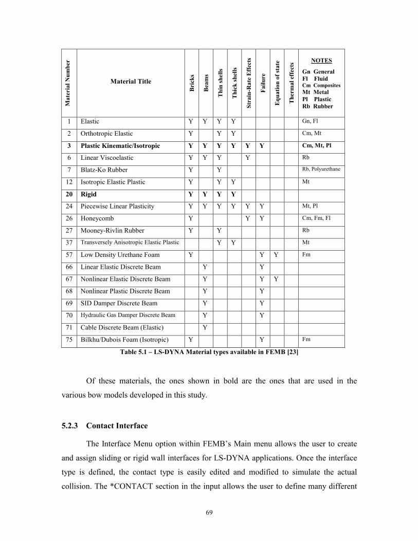
69
Mat
eria
l Num
ber
Material Title
Bric
ks
Beam
s
Thi
n sh
ells
Thi
ck sh
ells
Stra
in-R
ate
Effe
cts
Failu
re
Equ
atio
n of
stat
e
Ther
mal
effe
cts NOTES
Gn General Fl Fluid Cm Composites Mt Metal Pl Plastic Rb Rubber
1 Elastic Y Y Y Y Gn, Fl
2 Orthotropic Elastic Y Y Y Cm, Mt
3 Plastic Kinematic/Isotropic Y Y Y Y Y Y Cm, Mt, Pl
6 Linear Viscoelastic Y Y Y Y Rb
7 Blatz-Ko Rubber Y Y Rb, Polyurethane
12 Isotropic Elastic Plastic Y Y Y Mt
20 Rigid Y Y Y Y
24 Piecewise Linear Plasticity Y Y Y Y Y Y Mt, Pl
26 Honeycomb Y Y Y Cm, Fm, Fl
27 Mooney-Rivlin Rubber Y Y Rb
37 Transversely Anisotropic Elastic Plastic Y Y Mt
57 Low Density Urethane Foam Y Y Y Fm
66 Linear Elastic Discrete Beam Y Y
67 Nonlinear Elastic Discrete Beam Y Y Y
68 Nonlinear Plastic Discrete Beam Y Y
69 SID Damper Discrete Beam Y Y
70 Hydraulic Gas Damper Discrete Beam Y Y
71 Cable Discrete Beam (Elastic) Y
75 Bilkhu/Dubois Foam (Isotropic) Y Y Fm
Table 5.1 – LS-DYNA Material types available in FEMB [23]
Of these materials, the ones shown in bold are the ones that are used in the
various bow models developed in this study.
5.2.3 Contact Interface
The Interface Menu option within FEMB’s Main menu allows the user to create
and assign sliding or rigid wall interfaces for LS-DYNA applications. Once the interface
type is defined, the contact type is easily edited and modified to simulate the actual
collision. The *CONTACT section in the input allows the user to define many different
70
contact types. These contact options are for treating the contact of deformable bodies,
single surface contact in deformable bodies, and deformable body to rigid body contact.
The type of interface can be defined directly within FEMB, without the user having to
enter the input in KEYWORD format.
5.2.4 Specifications/database limitations
Currently FEMB has the following specifications/limitations per database:
200,000 POINTS
100,000 LINES
2,500 SURFACES
100,000 EDGE POINTS (SURFACE)
150,000 CONTROL POINTS (SURFACE)
100,000 GRIDS
225,000 ELEMENTS (Full Version)
10,000 ELEMENTS (Student Version)
1,000 PROPERTIES
1,000 PIDS
225,000 NODES
5.2.5 Line data
FEMB converts and filters the following (optional) line data to FEMB neutral line
format directly:
IGES (line and surface)
DXF (line data file format)
PDGS (standard format)
5.2.6 Recommended Practice (.fmb, .his, .lin, .bin, etc.)
To open/read files while in the FEMB program, the user should select File/Open from
the Main Menu bar. Specific file types would be listed within the Pop-Up menu. The
following extensions for specific file types is recommended:
71
• = FEMB database file name: filename.fmb
• = FEMB line data file name: filename.lin
• = IGES line/surface data name: filename.igs
• = DXF line data name: filename.dxf
• = PDGS line data: filename.pdgs
When reading a line data file into FEMB, the user should select File/Open from
the Main Menu bar. By default, all existing FEMB database files (*.fmb) will be listed.
Beneath the list of FEMB database files, there is a prompt for FILES OF TYPE. If the
user selects FEMB line data, all file names in that directory with the extension .lin will be
listed. The user may then select the appropriate file name. The user may choose ALL
FILES to display files with different extensions than those listed above.
5.2.7 Local coordinate system
FEMB refers to the local or global coordinate system to translate, rotate, mirror,
copy and generate points, lines, nodes and elements. When such a function is selected,
the program automatically prompts the user to generate a local coordinate system
designated as the U, V, W, coordinate frame.
One, two, or three reference points are required to establish a local coordinate
system. The first reference point defines the local origin. For a three point system the
second reference point defines the direction of the local U axis which is extended from
the first reference point. The third reference point, along with the first two reference
points, defines the local U-V plane. The local V axis is defined in the U-V plane and
perpendicular to the U axis. The local W axis is then defined according to the right hand
rule perpendicular to the U-V plane. For the two-reference point option, End Select
should be selected after the second reference point is defined. The local W axis lies along
the vector from the origin to the second reference point and the V axis lies in the V-W
plane. The U axis is defined by the right hand rule.
All rotational commands (i.e., generating arcs, copy with rotating, etc.) execute
around the local W or global Z-axes.
72
For a one-reference-point system, the user selects a point or node on the screen as
the local origin, and then selects one of the X, Y, or Z options available to define the
local W axis along one of the global axes.
5.2.8 Getting started with FEMB
There are three basic scenarios that the user will encounter when starting FEMB:
• = Supplied CAD line/surface data is read into FEMB.
• = Supplied model data (e.g., LS-DYNA, etc.) is read directly into FEMB.
• = CAD or model data is not supplied so the user starts with an empty database and
generates or 'digitizes' line data from a drawing.
5.2.9 Getting started with CAD data
In the LS-DYNA program manager, FEMB is started by clicking the Pre-/Post-
Processing button, or by pulling down the Builder/Viewer menu and selecting the Pre-
/Post-Processing menu item.
When reading a line data file into FEMB, by default all existing FEMB database
files (*.fmb) will be listed. Beneath the list of FEMB database files there is a prompt for
FILES OF TYPE. The user may select FEMB line data. All file names in that directory
with the extension .lin will be listed. The user may then select the appropriate file name.
Once the appropriate file has been selected, FEMB will create a database called
UNKNOWN.fmb containing the selected line data. The user may then save the database
under a new name. File types are read in directly without external translation.
When reading model data (LSDYNA type .dyn) into FEMB, by default, all
existing FEMB database files will be listed. Beneath the list of FEMB database files there
is a prompt for LIST OF FILE TYPE. The user may select the desired file type. All file
names in that directory with the extension .dyn will be listed. The user may then select
the appropriate file name. Once the appropriate file has been selected FEMB will create a
database called UNKNOWN.fmb containing the selected file type data. The user may
then save the database under a new name. File types are read in directly without external
translation.
73
In case CAD line data or model data from LSDYNA is not available, the user will
need to digitize a drawing thus generating one’s own line data. The line data can then be
modeled using FEMB. Once FEMB is started as described above, a window pops up
listing FEMB database files with the extension .fmb. Enter a new file name.
• = The first thing that needs to be done is to create a new part in the Part Menu.
FEMB will not allow entities to be created in an empty database unless there is an
existing part for the information.
• = Upon creating a new part, the user will be prompted, via Pop-Up window, to
define/assign material and element property. The user may either assign
properties or disregard this prompt by selecting the Cancel/End button. Once a
part has been created, the next step is to generate the desired line data.
• = Enter the Geom Menu (Geometry Builder).
• = Select the Generate Lines command and click the right most mouse button for the
available options.
• = Select KEY IN X, Y, Z if the coordinates of the line are known.
• = Once this is done the prompt will ask for the X, Y, Z coordinate. The prompt will
keep asking for the coordinates until you select End Select.
The user may continue generating line data or executing the other CAD functions
available in the menu.Generating a finite element model from line data is described in
Element Options (ELEM).
5.2.10 Main menu
This is the first menu the user sees when FEMB starts. The 15 initial options will
open an additional series of menus. The functions in the Main Menu are organized as
follows:
File - FILE MANAGER
Geom - GEOMETRY BUILDER
Surf - SURFACE MENU
Elem - ELEMENT OPTIONS
Node - NODE OPTIONS

74
Check - MODEL CHECKER
Part - PART CONTROL
Matl - MATERIAL PROPERTY
Prop - ELEMENT PROPERTY
I.F. - INTERFACE MENU
B.C. - BOUNDARY CONDITIONS
Set - LOAD SET
Help - “ABOUT” WINDOW
Figure 5.1 shows how the FEMB’s main menu looks and also, how the important
icons in the main menu look, and where they are located.
Figure 5.1 - Main Menu of FEMB
5.2.10.1 File menu
The options available in the File menu allow the user to input (open) data to or
output (save) data from FEMB. The user has the ability to input LS-DYNA, IGES, DXF,
LS-DYNA animation/graph data, and FEMB line data formats.
FILES OF TYPE allows the user to specify the type of file to open/save. The available
file types are:
FEMB Database *.fmb
FEMB Line *.lin
LS-DYNA *.dyn, *.dat
NASTRAN *.nas
IGES *.igs, *.iges
IDEA-S Universal *.unv
DXF *.dxf
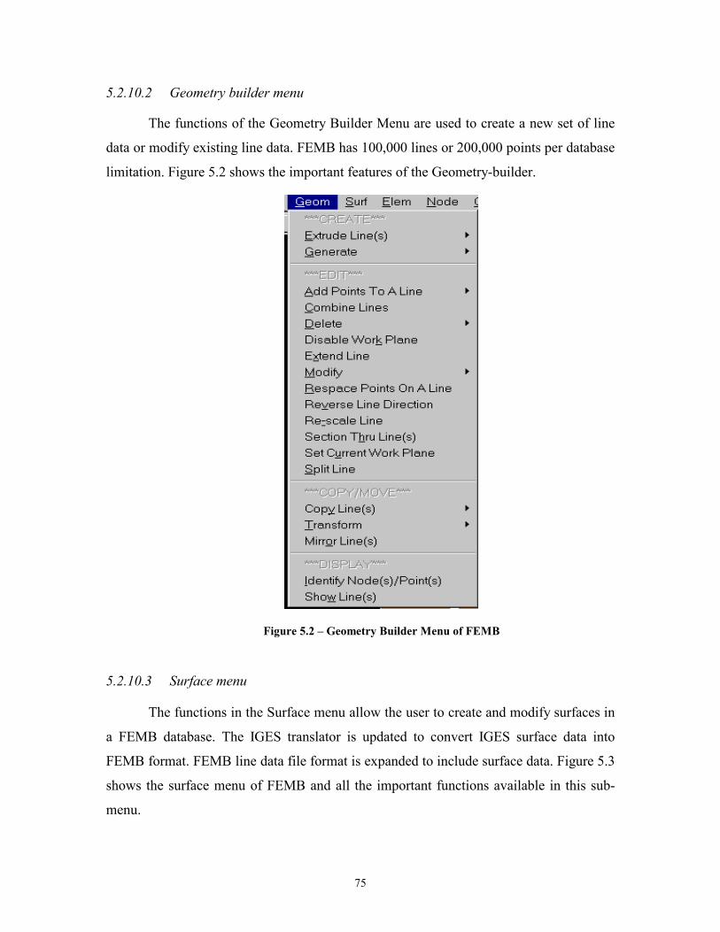
75
5.2.10.2 Geometry builder menu
The functions of the Geometry Builder Menu are used to create a new set of line
data or modify existing line data. FEMB has 100,000 lines or 200,000 points per database
limitation. Figure 5.2 shows the important features of the Geometry-builder.
Figure 5.2 – Geometry Builder Menu of FEMB
5.2.10.3 Surface menu
The functions in the Surface menu allow the user to create and modify surfaces in
a FEMB database. The IGES translator is updated to convert IGES surface data into
FEMB format. FEMB line data file format is expanded to include surface data. Figure 5.3
shows the surface menu of FEMB and all the important functions available in this sub-
menu.
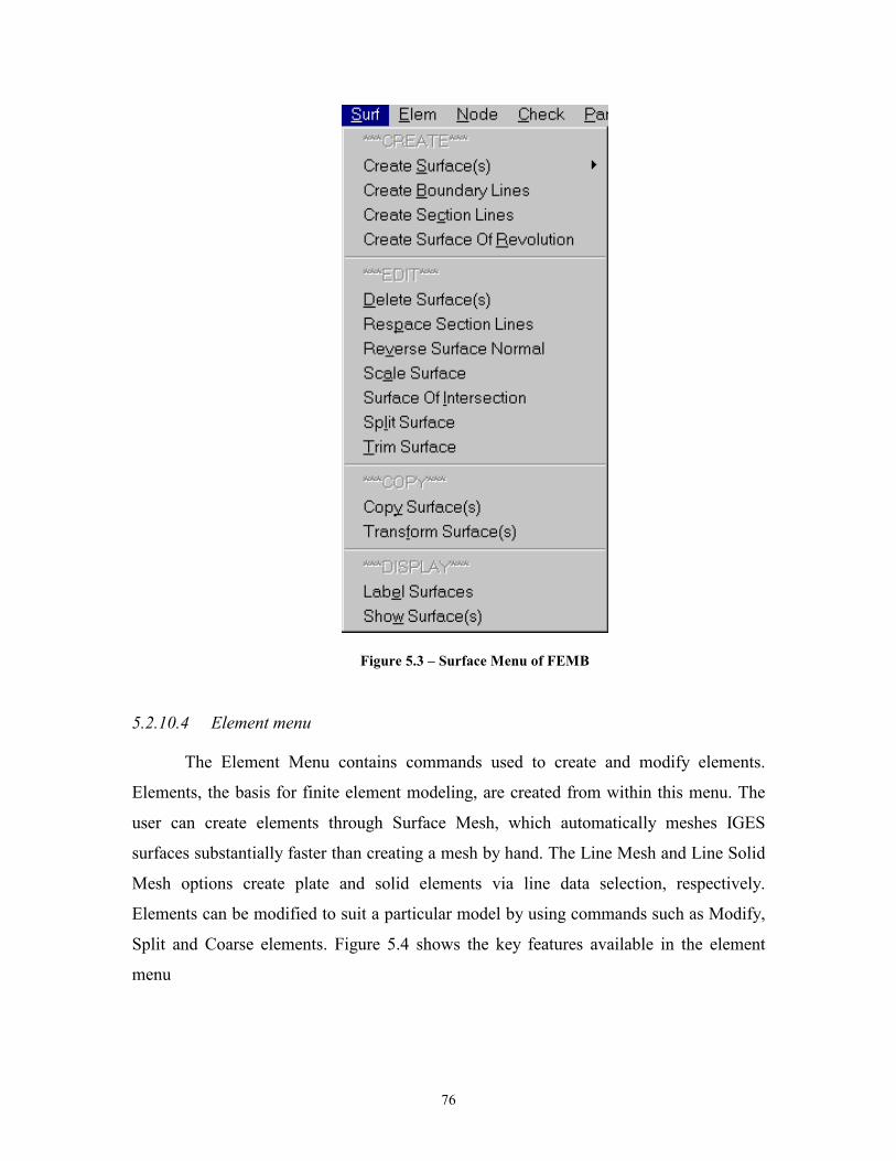
76
Figure 5.3 – Surface Menu of FEMB
5.2.10.4 Element menu
The Element Menu contains commands used to create and modify elements.
Elements, the basis for finite element modeling, are created from within this menu. The
user can create elements through Surface Mesh, which automatically meshes IGES
surfaces substantially faster than creating a mesh by hand. The Line Mesh and Line Solid
Mesh options create plate and solid elements via line data selection, respectively.
Elements can be modified to suit a particular model by using commands such as Modify,
Split and Coarse elements. Figure 5.4 shows the key features available in the element
menu
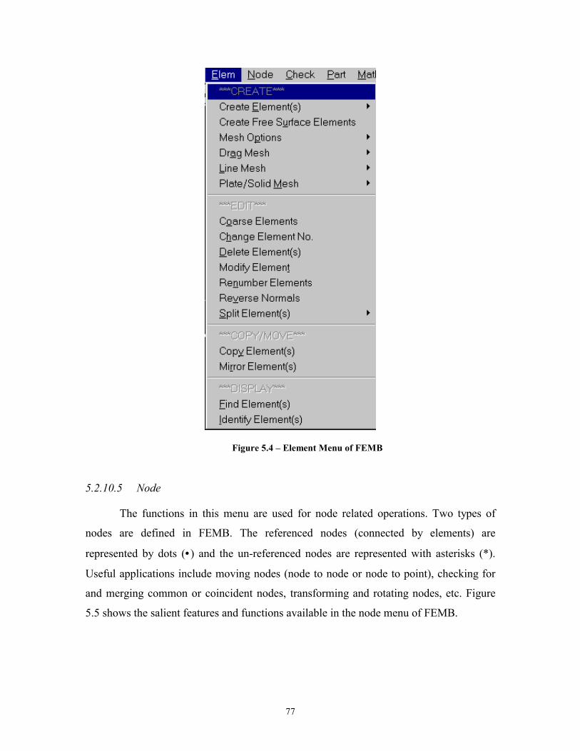
77
Figure 5.4 – Element Menu of FEMB
5.2.10.5 Node
The functions in this menu are used for node related operations. Two types of
nodes are defined in FEMB. The referenced nodes (connected by elements) are
represented by dots (• ) and the un-referenced nodes are represented with asterisks (*).
Useful applications include moving nodes (node to node or node to point), checking for
and merging common or coincident nodes, transforming and rotating nodes, etc. Figure
5.5 shows the salient features and functions available in the node menu of FEMB.
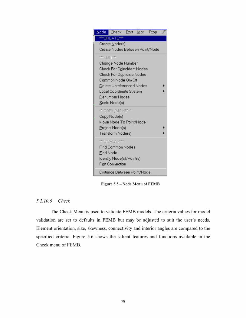
78
Figure 5.5 – Node Menu of FEMB
5.2.10.6 Check
The Check Menu is used to validate FEMB models. The criteria values for model
validation are set to defaults in FEMB but may be adjusted to suit the user’s needs.
Element orientation, size, skewness, connectivity and interior angles are compared to the
specified criteria. Figure 5.6 shows the salient features and functions available in the
Check menu of FEMB.
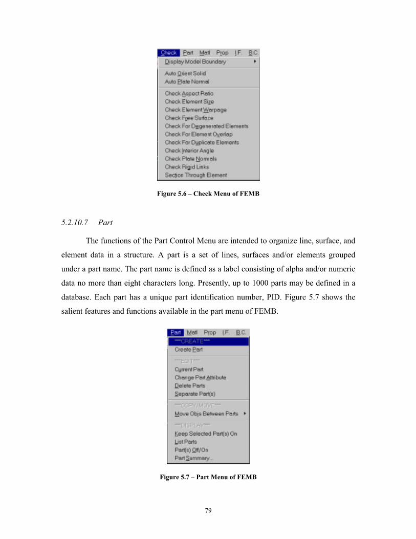
79
Figure 5.6 – Check Menu of FEMB
5.2.10.7 Part
The functions of the Part Control Menu are intended to organize line, surface, and
element data in a structure. A part is a set of lines, surfaces and/or elements grouped
under a part name. The part name is defined as a label consisting of alpha and/or numeric
data no more than eight characters long. Presently, up to 1000 parts may be defined in a
database. Each part has a unique part identification number, PID. Figure 5.7 shows the
salient features and functions available in the part menu of FEMB.
Figure 5.7 – Part Menu of FEMB
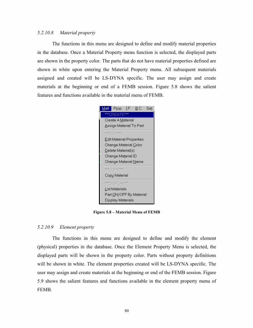
80
5.2.10.8 Material property
The functions in this menu are designed to define and modify material properties
in the database. Once a Material Property menu function is selected, the displayed parts
are shown in the property color. The parts that do not have material properties defined are
shown in white upon entering the Material Property menu. All subsequent materials
assigned and created will be LS-DYNA specific. The user may assign and create
materials at the beginning or end of a FEMB session. Figure 5.8 shows the salient
features and functions available in the material menu of FEMB.
Figure 5.8 – Material Menu of FEMB
5.2.10.9 Element property
The functions in this menu are designed to define and modify the element
(physical) properties in the database. Once the Element Property Menu is selected, the
displayed parts will be shown in the property color. Parts without property definitions
will be shown in white. The element properties created will be LS-DYNA specific. The
user may assign and create materials at the beginning or end of the FEMB session. Figure
5.9 shows the salient features and functions available in the element property menu of
FEMB.
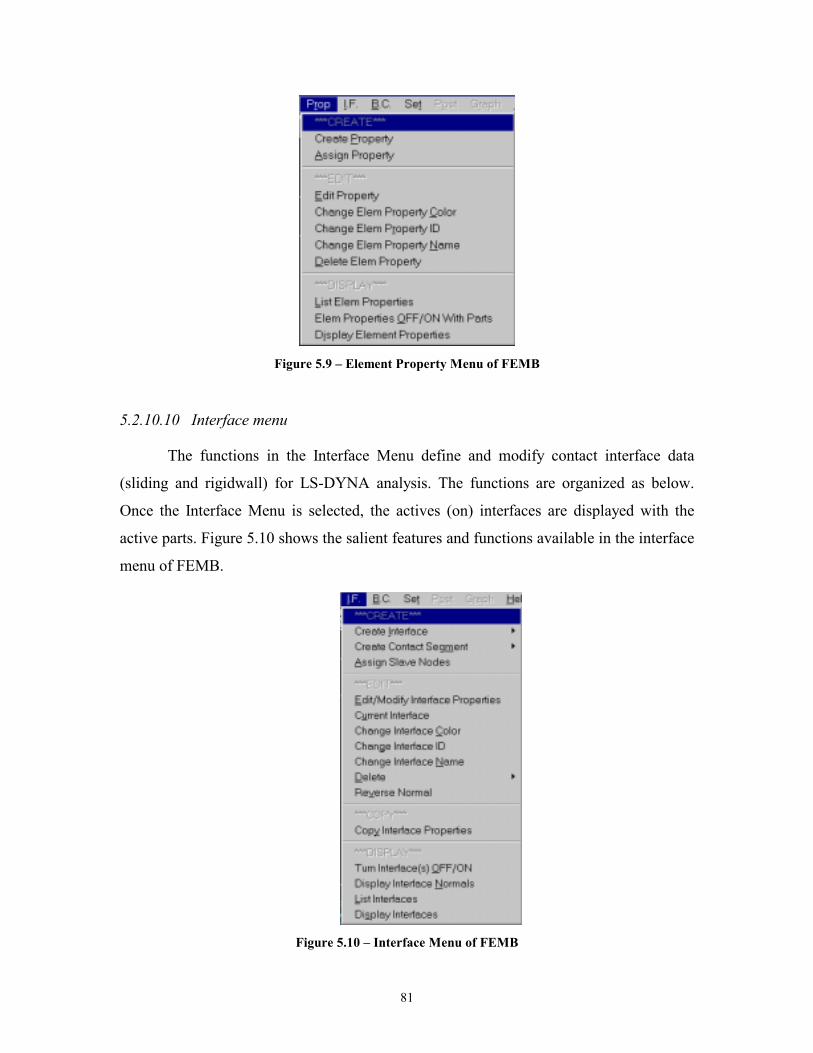
81
Figure 5.9 – Element Property Menu of FEMB
5.2.10.10 Interface menu
The functions in the Interface Menu define and modify contact interface data
(sliding and rigidwall) for LS-DYNA analysis. The functions are organized as below.
Once the Interface Menu is selected, the actives (on) interfaces are displayed with the
active parts. Figure 5.10 shows the salient features and functions available in the interface
menu of FEMB.
Figure 5.10 – Interface Menu of FEMB
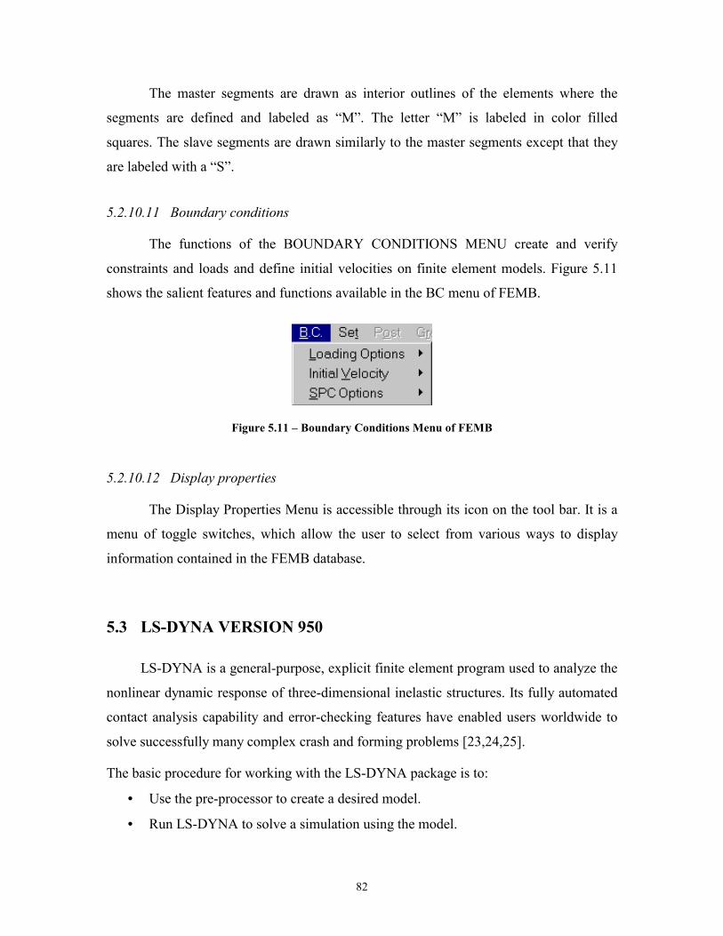
82
The master segments are drawn as interior outlines of the elements where the
segments are defined and labeled as “M”. The letter “M” is labeled in color filled
squares. The slave segments are drawn similarly to the master segments except that they
are labeled with a “S”.
5.2.10.11 Boundary conditions
The functions of the BOUNDARY CONDITIONS MENU create and verify
constraints and loads and define initial velocities on finite element models. Figure 5.11
shows the salient features and functions available in the BC menu of FEMB.
Figure 5.11 – Boundary Conditions Menu of FEMB
5.2.10.12 Display properties
The Display Properties Menu is accessible through its icon on the tool bar. It is a
menu of toggle switches, which allow the user to select from various ways to display
information contained in the FEMB database.
5.3 LS-DYNA VERSION 950
LS-DYNA is a general-purpose, explicit finite element program used to analyze the
nonlinear dynamic response of three-dimensional inelastic structures. Its fully automated
contact analysis capability and error-checking features have enabled users worldwide to
solve successfully many complex crash and forming problems [23,24,25].
The basic procedure for working with the LS-DYNA package is to:
• = Use the pre-processor to create a desired model.
• = Run LS-DYNA to solve a simulation using the model.
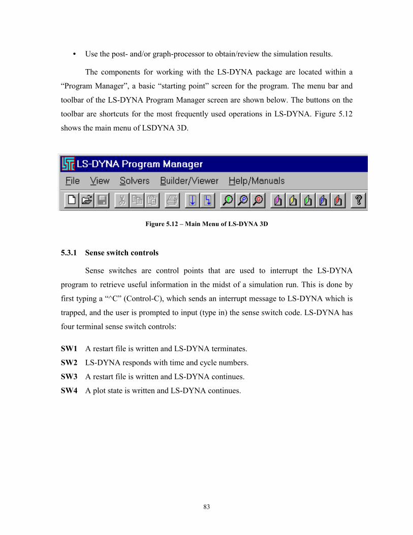
83
• = Use the post- and/or graph-processor to obtain/review the simulation results.
The components for working with the LS-DYNA package are located within a
“Program Manager”, a basic “starting point” screen for the program. The menu bar and
toolbar of the LS-DYNA Program Manager screen are shown below. The buttons on the
toolbar are shortcuts for the most frequently used operations in LS-DYNA. Figure 5.12
shows the main menu of LSDYNA 3D.
Figure 5.12 – Main Menu of LS-DYNA 3D
5.3.1 Sense switch controls
Sense switches are control points that are used to interrupt the LS-DYNA
program to retrieve useful information in the midst of a simulation run. This is done by
first typing a “^C” (Control-C), which sends an interrupt message to LS-DYNA which is
trapped, and the user is prompted to input (type in) the sense switch code. LS-DYNA has
four terminal sense switch controls:
SW1 A restart file is written and LS-DYNA terminates.
SW2 LS-DYNA responds with time and cycle numbers.
SW3 A restart file is written and LS-DYNA continues.
SW4 A plot state is written and LS-DYNA continues.
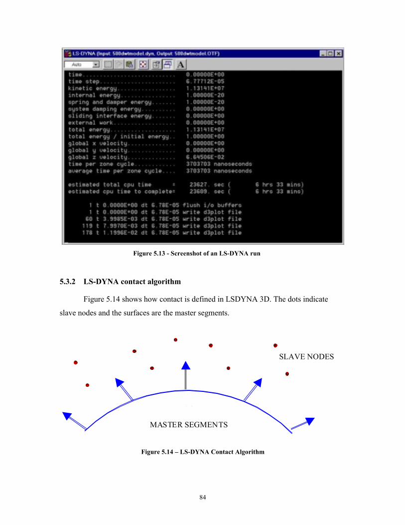
84
Figure 5.13 - Screenshot of an LS-DYNA run
5.3.2 LS-DYNA contact algorithm
Figure 5.14 shows how contact is defined in LSDYNA 3D. The dots indicate
slave nodes and the surfaces are the master segments.
6 46 3
6 26 1
MASTER SEGMENTS
SLAVE NODES
Figure 5.14 – LS-DYNA Contact Algorithm
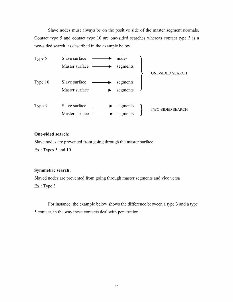
85
Slave nodes must always be on the positive side of the master segment normals.
Contact type 5 and contact type 10 are one-sided searches whereas contact type 3 is a
two-sided search, as described in the example below.
Type 5 Slave surface nodes
Master surface segments
Type 10 Slave surface segments
Master surface segments
Type 3 Slave surface segments
Master surface segments
One-sided search:
Slave nodes are prevented from going through the master surface
Ex.: Types 5 and 10
Symmetric search:
Slaved nodes are prevented from going through master segments and vice versa
Ex.: Type 3
For instance, the example below shows the difference between a type 3 and a type
5 contact, in the way these contacts deal with penetration.
ONE-SIDED SEARCH
TWO-SIDED SEARCH
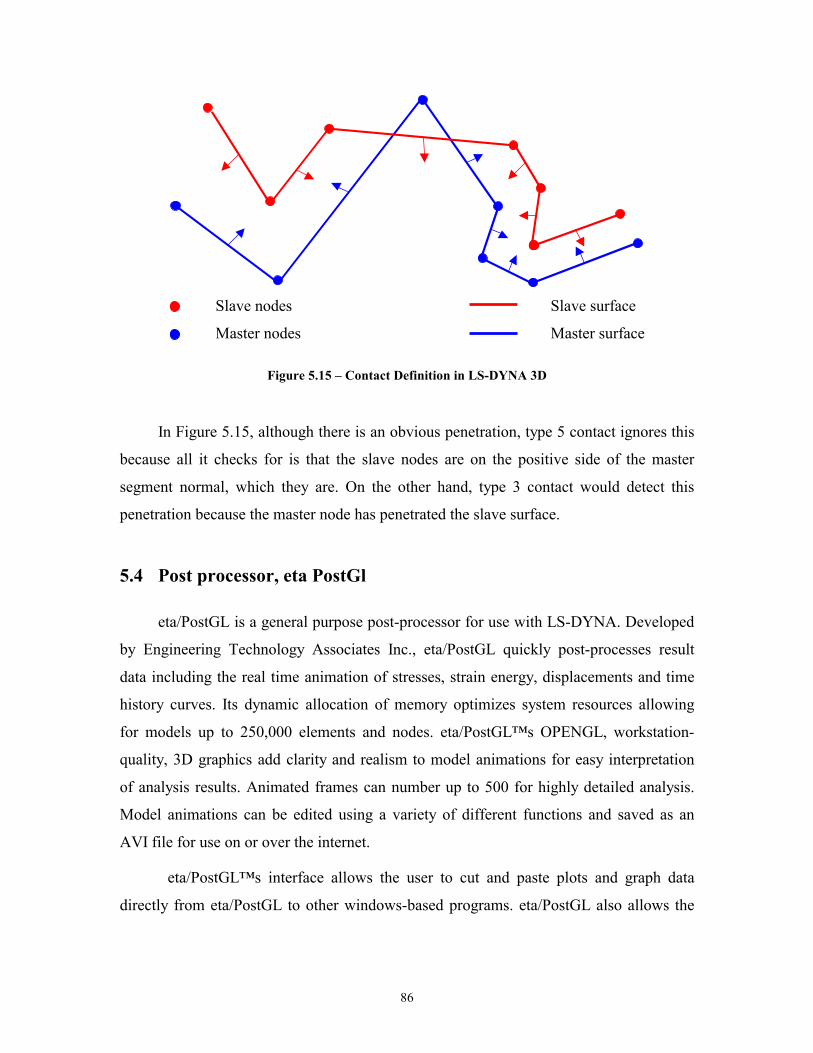
86
Slave nodes Slave surface
Master nodes Master surface
Figure 5.15 – Contact Definition in LS-DYNA 3D
In Figure 5.15, although there is an obvious penetration, type 5 contact ignores this
because all it checks for is that the slave nodes are on the positive side of the master
segment normal, which they are. On the other hand, type 3 contact would detect this
penetration because the master node has penetrated the slave surface.
5.4 Post processor, eta PostGl
eta/PostGL is a general purpose post-processor for use with LS-DYNA. Developed
by Engineering Technology Associates Inc., eta/PostGL quickly post-processes result
data including the real time animation of stresses, strain energy, displacements and time
history curves. Its dynamic allocation of memory optimizes system resources allowing
for models up to 250,000 elements and nodes. eta/PostGL™s OPENGL, workstation-
quality, 3D graphics add clarity and realism to model animations for easy interpretation
of analysis results. Animated frames can number up to 500 for highly detailed analysis.
Model animations can be edited using a variety of different functions and saved as an
AVI file for use on or over the internet.
eta/PostGL™s interface allows the user to cut and paste plots and graph data
directly from eta/PostGL to other windows-based programs. eta/PostGL also allows the
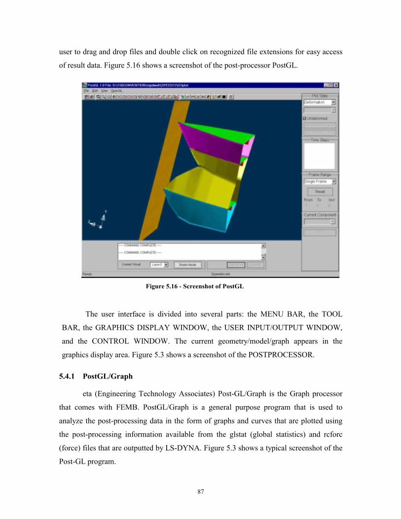
87
user to drag and drop files and double click on recognized file extensions for easy access
of result data. Figure 5.16 shows a screenshot of the post-processor PostGL.
Figure 5.16 - Screenshot of PostGL
The user interface is divided into several parts: the MENU BAR, the TOOL
BAR, the GRAPHICS DISPLAY WINDOW, the USER INPUT/OUTPUT WINDOW,
and the CONTROL WINDOW. The current geometry/model/graph appears in the
graphics display area. Figure 5.3 shows a screenshot of the POSTPROCESSOR.
5.4.1 PostGL/Graph
eta (Engineering Technology Associates) Post-GL/Graph is the Graph processor
that comes with FEMB. PostGL/Graph is a general purpose program that is used to
analyze the post-processing data in the form of graphs and curves that are plotted using
the post-processing information available from the glstat (global statistics) and rcforc
(force) files that are outputted by LS-DYNA. Figure 5.3 shows a typical screenshot of the
Post-GL program.
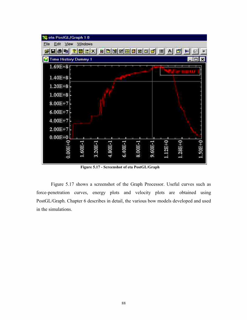
88
Figure 5.17 - Screenshot of eta PostGL/Graph
Figure 5.17 shows a screenshot of the Graph Processor. Useful curves such as
force-penetration curves, energy plots and velocity plots are obtained using
PostGL/Graph. Chapter 6 describes in detail, the various bow models developed and used
in the simulations.
89
Chapter 6 Bow and Hull Models Developed in LSDYNA 6.1 Introduction
This chapter describes the methodology used to develop bow and hull models in
LS-DYNA. Table 6.1 lists the various models that were developed. The principal
characteristics, bow profile, structural design and scantlings for the striking bows and
struck tankers used in this study are provided in Section 6.3.2, Section 6.3.3 and
Appendix B. The striking ships include a 500 dwt coaster, 23000 dwt containership,
40000 dwt containership and a 150000 dwt bulk carrier. The struck ships include a
150000 dwt double hull tanker (DH150) and a 100000 dwt single hull tanker (SH100).
6.2 Test case matrix
Cases I-1 to I-4 in Table 6.1 use the closed-form Yang and Caldwell equation [70]
to calculate force versus deflection for the bows striking a rigid wall at different speeds.
This equation sums the force-deflection behavior of individual intersection elements.
These calculations are provided in Appendix A. Cases I-5 to I-8 use “intersection”-
elements in an LS-DYNA course-mesh finite element analysis to model the bows striking
a rigid wall at different speeds. The cross-sectional area of these elements is chosen to
duplicate the intersection element stiffness as calculated using the Yang and Caldwell
equation [70]. Actual plastic material properties are used, and element areas are
calculated to match element terms in Yang and Caldwell. These calculations are also
provided in Appendix A.
In Cases I-9 and I-10, the LSDYNA intersection element model of the 23000 dwt
containership strikes a conventional SH100 model at 5m/s. The conventional models use
a fine mesh and Belytscko-Tsay shell elements. SH100 is fixed in Case I-9 and free-in-
sway only in Case I-10. In Cases I-11 and I-12 the LSDYNA intersection element model
of the 150000 dwt bulk carrier strikes the conventional DH150 at 5m/s. DH150 is fixed
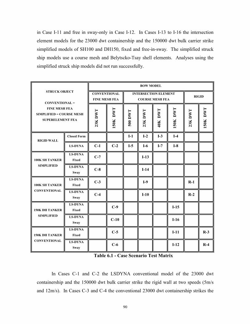
90
in Case I-11 and free in sway-only in Case I-12. In Cases I-13 to I-16 the intersection
element models for the 23000 dwt containership and the 150000 dwt bulk carrier strike
simplified models of SH100 and DH150, fixed and free-in-sway. The simplified struck
ship models use a course mesh and Belytscko-Tsay shell elements. Analyses using the
simplified struck ship models did not run successfully.
BOW MODEL
CONVENTIONAL
FINE MESH FEA
INTERSECTION ELEMENT
COURSE MESH FEA RIGID
STRUCK OBJECT
CONVENTIONAL =
FINE MESH FEA
SIMPLIFIED = COURSE MESH
SUPERELEMENT FEA
23K
DW
T
150K
DW
T
500
DW
T
23K
DW
T
40K
DW
T
150K
DW
T
23K
DW
T
150K
DW
T
Closed Form I-1 I-2 I-3 I-4
RIGID WALL LS-DYNA C-1 C-2 I-5 I-6 I-7 I-8 LS-DYNA
Fixed C-7 I-13
100K SH TANKER
SIMPLIFIED LS-DYNA
Sway C-8 I-14
LS-DYNA
Fixed C-3 I-9 R-1
100K SH TANKER
CONVENTIONAL LS-DYNA
Sway C-4 I-10 R-2
LS-DYNA
Fixed C-9 I-15
150K DH TANKER
SIMPLIFIED LS-DYNA
Sway C-10 I-16
LS-DYNA
Fixed C-5 I-11 R-3
150K DH TANKER
CONVENTIONAL LS-DYNA
Sway C-6 I-12 R-4
Table 6.1 - Case Scenario Test Matrix
In Cases C-1 and C-2 the LSDYNA conventional model of the 23000 dwt
containership and the 150000 dwt bulk carrier strike the rigid wall at two speeds (5m/s
and 12m/s). In Cases C-3 and C-4 the conventional 23000 dwt containership strikes the
91
conventional SH100 at two speeds (5m/s and 12m/s), in fixed and sway-only conditions.
In Cases C-5 and C-6 conventional models of the 150000 dwt bulk carrier strike the
conventional DH150 at 5m/s, in fixed and sway-only conditions. In Cases C-7 to C-10
the conventional 23000 dwt containership and the conventional 150000 dwt bulk carrier
strike the simplified SH100 and DH150, in fixed and sway-only conditions. These cases
using the simplified struck ship models also did not run successfully.
In Cases R-1 through R-4 a rigid 23000 dwt containership and a rigid 150000 dwt
bulk carrier strike the conventional SH100 and DH100. These tests were run to compare
rigid bow collision results in LSDYNA to those calculated using SIMCOL, which also
assumes a rigid bow.
6.3 GENERAL MODEL DESCRIPTION
This section describes the general modeling features common to all the cases. A
flowchart showing the important steps in developing the various models is shown in
Figure 6.1. Section 6.4 discusses the important modeling parameters specific to each of
the eighteen cases.
6.3.1 Bow and the Side Structure Drawings
The bow model of the 500 dwt striking bow was created using AutoCAD-R14
and saved as a .DXF file that was later imported to the pre-processor FEMB. This file
was then saved as an FEMB line data file (.LIN). After developing expertise in FEMB,
the remaining bow models and side-ship models are created using the geometry builder
features of FEMB in order to avoid exporting and importing of CAD line data. Principal
particulars and dimensions for the striking ships were taken from Pedersen [52], as
detailed in Section 6.3.2 and Appendix B. Section 6.3.3 and Appendix B provide
characteristics of the struck ships.
6.3.2 Bow Geometry
Various bow models are analyzed as part of this thesis. Four different ships are
considered: a 500 dwt coaster, 23000 dwt containership, 40000 dwt containership and a
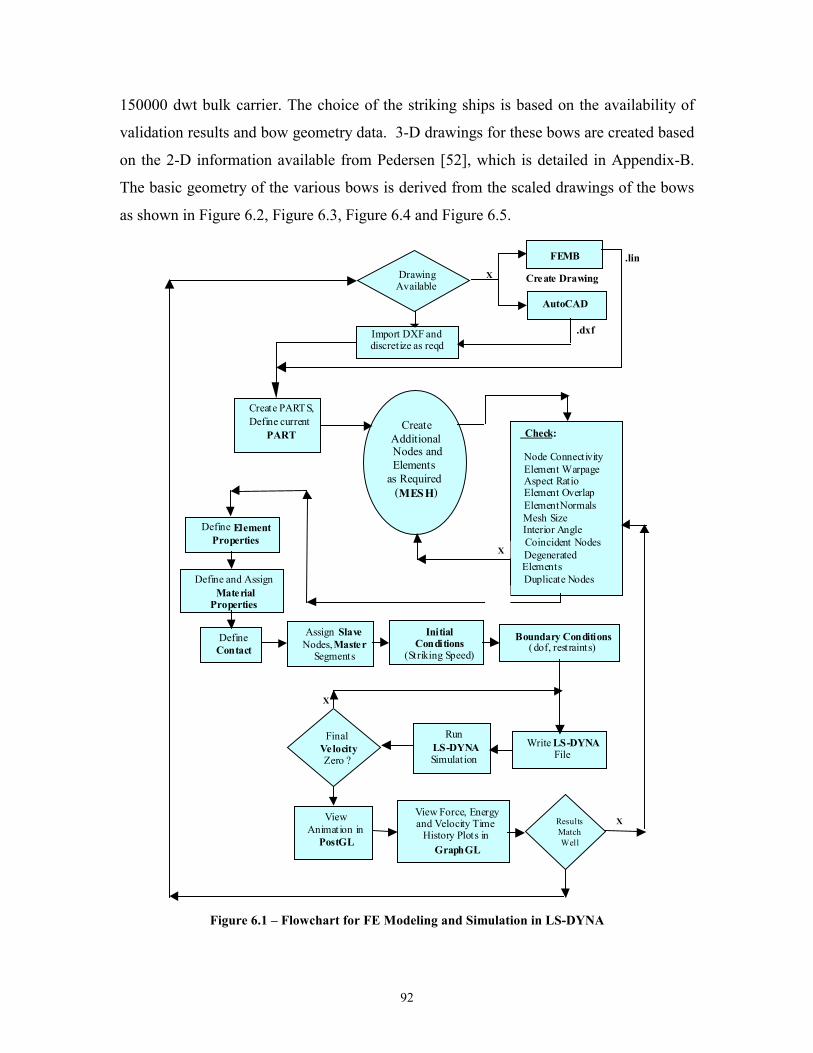
92
150000 dwt bulk carrier. The choice of the striking ships is based on the availability of
validation results and bow geometry data. 3-D drawings for these bows are created based
on the 2-D information available from Pedersen [52], which is detailed in Appendix-B.
The basic geometry of the various bows is derived from the scaled drawings of the bows
as shown in Figure 6.2, Figure 6.3, Figure 6.4 and Figure 6.5.
Create PARTS, Define current
PART
Initial Conditions
(Striking Speed) Boundary Conditions
( dof, restraints) Define Contact
Assign Slave Nodes, Master
Segments
Define and Assign Material
Properties
Define Element Properties
Write LS-DYNA File
Run LS-DYNA Simulat ion
Final Velocity Zero ?
X
View Animation in
PostGL
View Force, Energy and Velocity Time
History Plots in GraphGL
Results Match Well
X
Drawing Available
Import DXF and discretize as reqd
X
AutoCAD
Check: Node Connectivity Element Warpage Aspect Ratio Element Overlap Element Normals Mesh Size Interior Angle Coincident Nodes Degenerated Elements Duplicate Nodes
Create Additional Nodes and Elements
as Required ( MESH )
X
FEMB Create Drawing
.lin
.dxf
Figure 6.1 – Flowchart for FE Modeling and Simulation in LS-DYNA
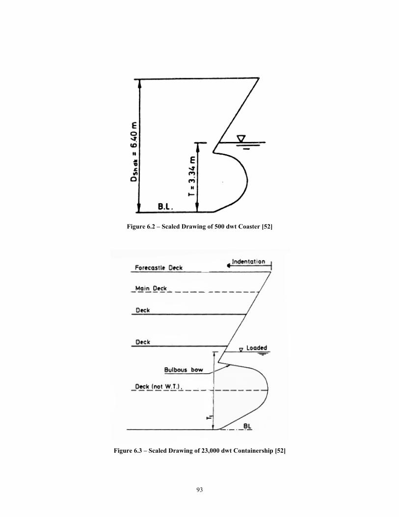
93
Figure 6.2 – Scaled Drawing of 500 dwt Coaster [52]
Figure 6.3 – Scaled Drawing of 23,000 dwt Containership [52]
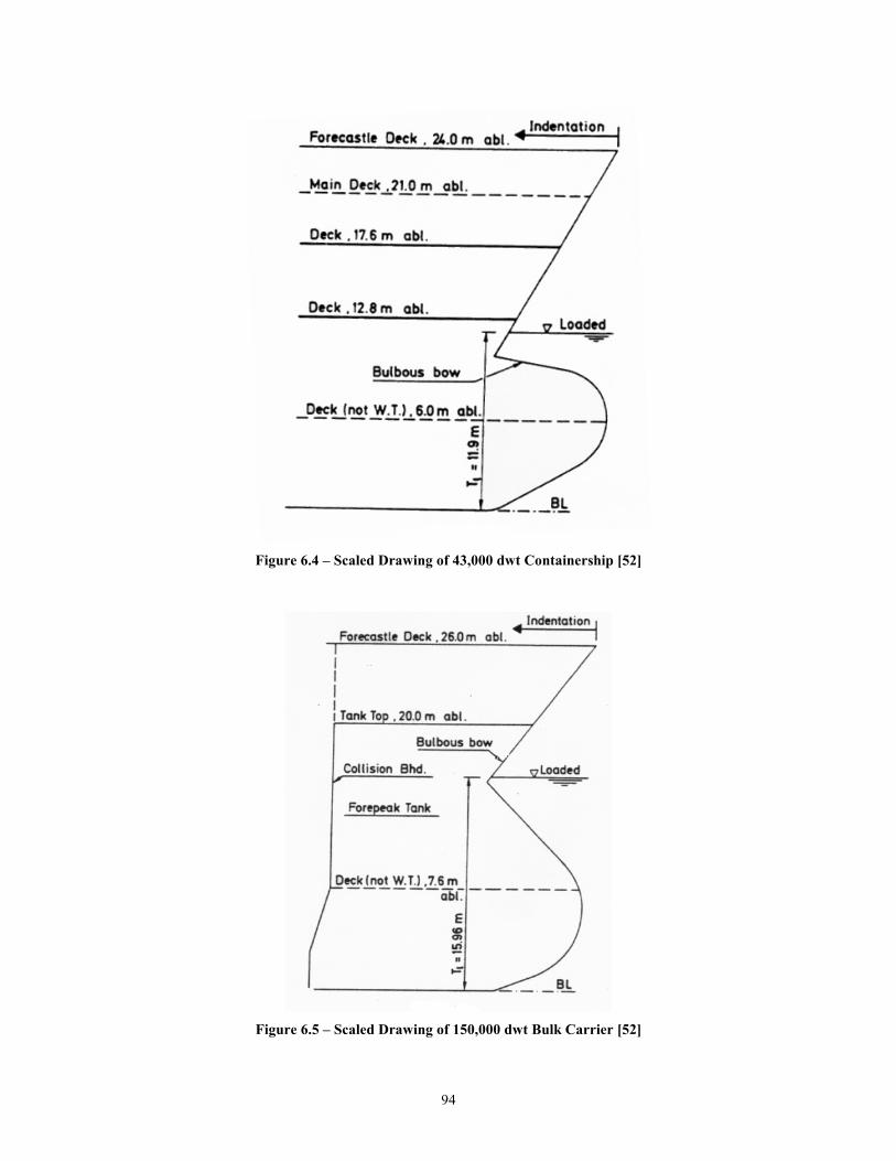
94
Figure 6.4 – Scaled Drawing of 43,000 dwt Containership [52]
Figure 6.5 – Scaled Drawing of 150,000 dwt Bulk Carrier [52]
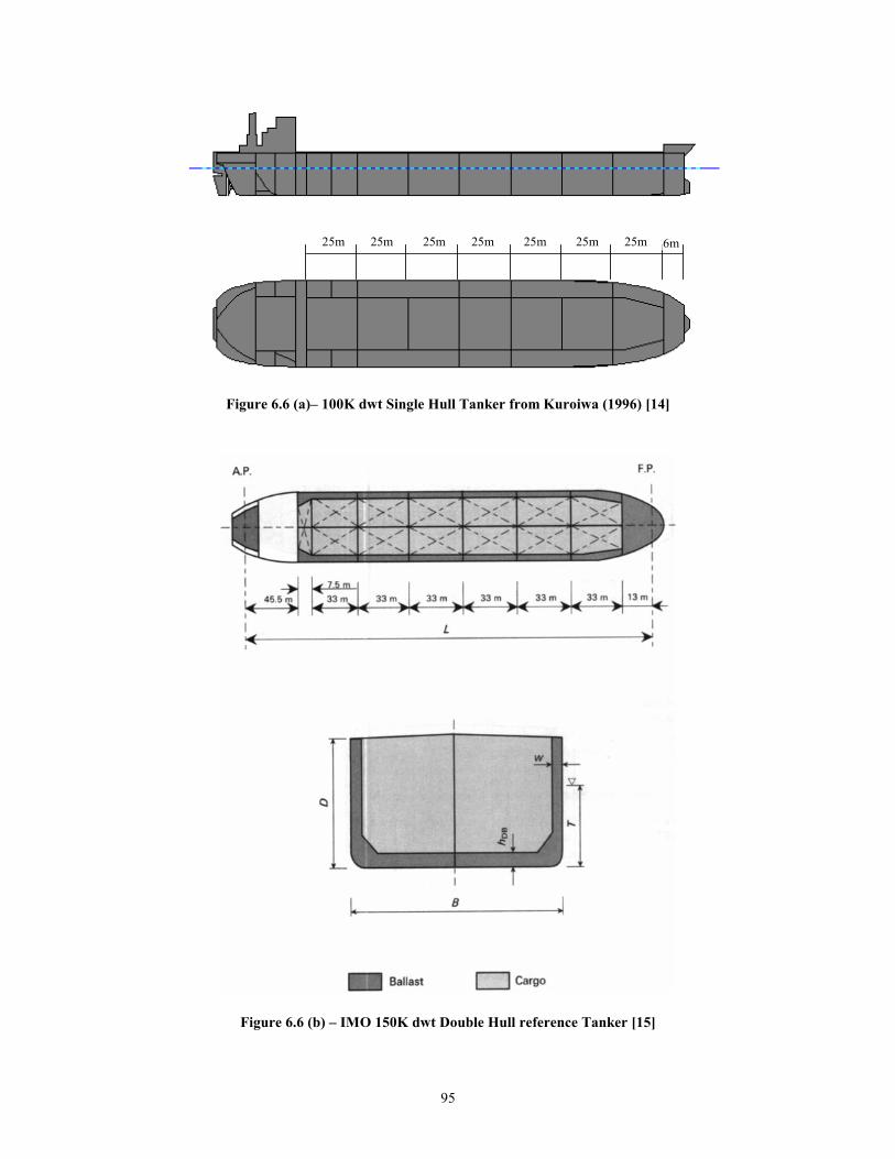
95
6m25m 25m 25m 25m 25m 25m 25m
Figure 6.6 (a)– 100K dwt Single Hull Tanker from Kuroiwa (1996) [14]
Figure 6.6 (b) – IMO 150K dwt Double Hull reference Tanker [15]
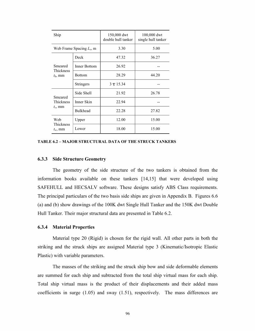
96
Ship 150,000 dwtdouble hull tanker
100,000 dwtsingle hull tanker
Web Frame Spacing Ls, m 3.30 5.00
Deck 47.32 36.27
Inner Bottom 26.92 --
Bottom 28.29 44.20
SmearedThicknessth, mm
Stringers 3 “ 15.34 --
Side Shell 21.92 26.78
Inner Skin 22.94 --SmearedThicknesstv, mm
Bulkhead 22.28 27.82
Upper 12.00 15.00WebThicknesstw, mm Lower 18.00 15.00
TABLE 6.2 – MAJOR STRUCTURAL DATA OF THE STRUCK TANKERS
6.3.3 Side Structure Geometry
The geometry of the side structure of the two tankers is obtained from the
information books available on these tankers [14,15] that were developed using
SAFEHULL and HECSALV software. These designs satisfy ABS Class requirements.
The principal particulars of the two basis side ships are given in Appendix B. Figures 6.6
(a) and (b) show drawings of the 100K dwt Single Hull Tanker and the 150K dwt Double
Hull Tanker. Their major structural data are presented in Table 6.2.
6.3.4 Material Properties
Material type 20 (Rigid) is chosen for the rigid wall. All other parts in both the
striking and the struck ships are assigned Material type 3 (Kinematic/Isotropic Elastic
Plastic) with variable parameters.
The masses of the striking and the struck ship bow and side deformable elements
are summed for each ship and subtracted from the total ship virtual mass for each ship.
Total ship virtual mass is the product of their displacements and their added mass
coefficients in surge (1.05) and sway (1.51), respectively. The mass differences are
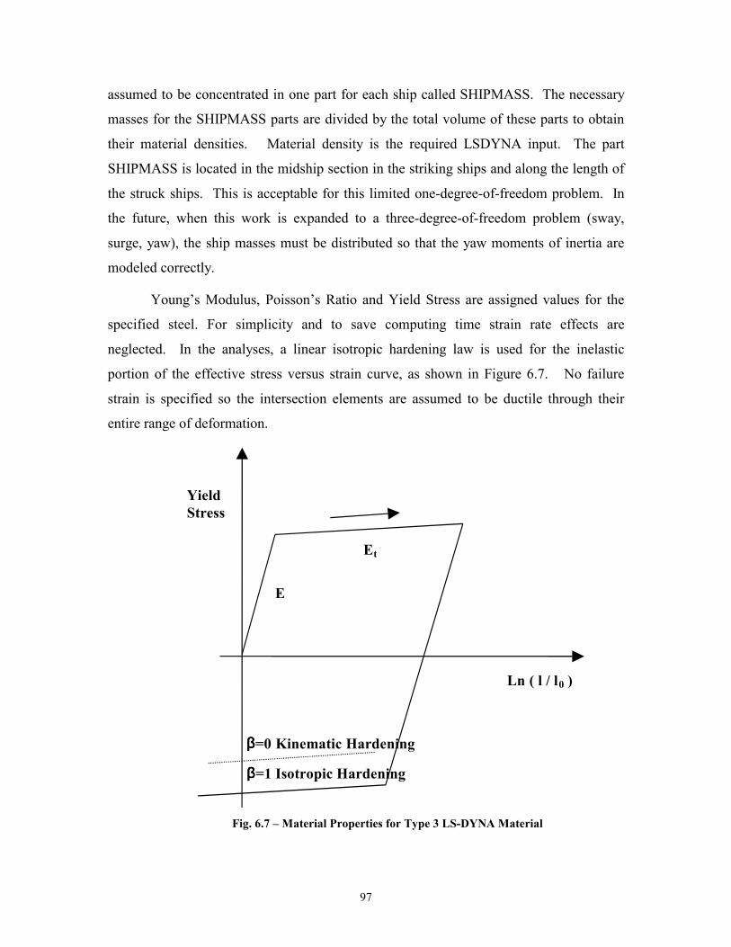
97
assumed to be concentrated in one part for each ship called SHIPMASS. The necessary
masses for the SHIPMASS parts are divided by the total volume of these parts to obtain
their material densities. Material density is the required LSDYNA input. The part
SHIPMASS is located in the midship section in the striking ships and along the length of
the struck ships. This is acceptable for this limited one-degree-of-freedom problem. In
the future, when this work is expanded to a three-degree-of-freedom problem (sway,
surge, yaw), the ship masses must be distributed so that the yaw moments of inertia are
modeled correctly.
Young’s Modulus, Poisson’s Ratio and Yield Stress are assigned values for the
specified steel. For simplicity and to save computing time strain rate effects are
neglected. In the analyses, a linear isotropic hardening law is used for the inelastic
portion of the effective stress versus strain curve, as shown in Figure 6.7. No failure
strain is specified so the intersection elements are assumed to be ductile through their
entire range of deformation.
ββββ=0 Kinematic Hardening
YieldStress
E
Et
Ln ( l / l0 )
ββββ=1 Isotropic Hardening
Fig. 6.7 – Material Properties for Type 3 LS-DYNA Material
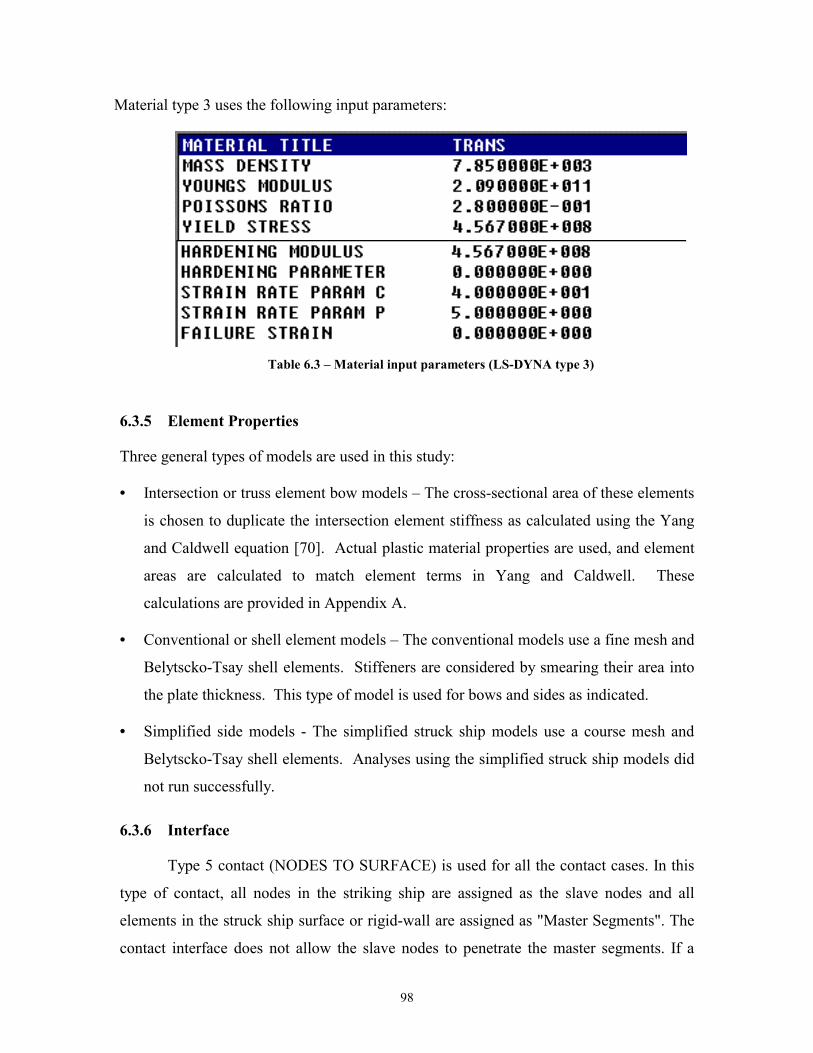
98
Material type 3 uses the following input parameters:
Table 6.3 – Material input parameters (LS-DYNA type 3)
6.3.5 Element Properties
Three general types of models are used in this study:
• = Intersection or truss element bow models – The cross-sectional area of these elements
is chosen to duplicate the intersection element stiffness as calculated using the Yang
and Caldwell equation [70]. Actual plastic material properties are used, and element
areas are calculated to match element terms in Yang and Caldwell. These
calculations are provided in Appendix A.
• = Conventional or shell element models – The conventional models use a fine mesh and
Belytscko-Tsay shell elements. Stiffeners are considered by smearing their area into
the plate thickness. This type of model is used for bows and sides as indicated.
• = Simplified side models - The simplified struck ship models use a course mesh and
Belytscko-Tsay shell elements. Analyses using the simplified struck ship models did
not run successfully.
6.3.6 Interface
Type 5 contact (NODES TO SURFACE) is used for all the contact cases. In this
type of contact, all nodes in the striking ship are assigned as the slave nodes and all
elements in the struck ship surface or rigid-wall are assigned as "Master Segments". The
contact interface does not allow the slave nodes to penetrate the master segments. If a
99
rigid wall is defined as the master, then the striking ship must deform because of the
contact definition. If the struck ship is assigned as the master, both the ships must deform
because the slave nodes are not allowed to penetrate the master surfaces.
6.3.7 Boundary Conditions
The motion of the bow is restricted to the direction perpendicular to the un-
deformed outer shell of the struck ship or rigid wall. Only collisions at right angles are
considered. If this restraint is not imposed on the bow model, it was observed that the
simulation results in modes of geometric unfeasibility. Various other dof combinations
were tried. Until this limitation is removed, oblique collision angles cannot be
considered. This will be addressed in future work.
The boundary conditions on the struck ship in the fixed case have all degrees of
freedom fixed for the nodes lying on the centerline of the struck ship. Other nodes have
only one dof, in the transverse direction of collision. In the case where sway is
considered, the fixed nodes are released and are given one dof, in the sway direction.
The ship mass is adjusted to include added mass in sway.
6.3.8 Initial Conditions
The initial velocity assigned to the nodes of the bow is equal to the speed of the
striking vessel before collision. In some cases, this parameter has been varied to see the
sensitivity of results to this variation. A velocity equaling the ship velocity is assigned to
all nodes in the striking ship. Striking velocities of 5m/s and 12m/s are chosen for the
analysis so that results can be compared with those from Pedersen [52].
6.3.9 Element Size
The accuracy of the results in finite element calculations generally increases if
smaller elements are used. The size of the elements in the bow intersection models and
the simplified side models are determined by their ship geometry’s. They are both very
course-mesh super-element models. The intersection bow models work very well
because the intersection elements are true and valid super-elements. The simplified side
models are not satisfactory because valid side panel super-elements are not currently
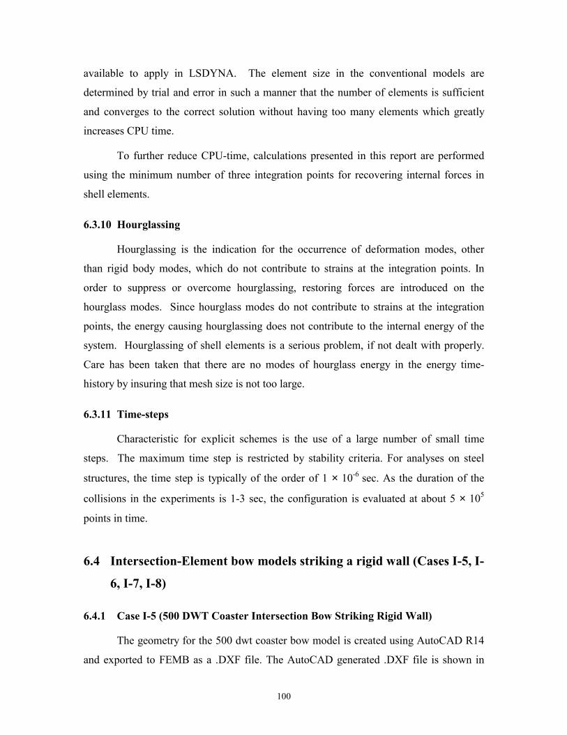
100
available to apply in LSDYNA. The element size in the conventional models are
determined by trial and error in such a manner that the number of elements is sufficient
and converges to the correct solution without having too many elements which greatly
increases CPU time.
To further reduce CPU-time, calculations presented in this report are performed
using the minimum number of three integration points for recovering internal forces in
shell elements.
6.3.10 Hourglassing
Hourglassing is the indication for the occurrence of deformation modes, other
than rigid body modes, which do not contribute to strains at the integration points. In
order to suppress or overcome hourglassing, restoring forces are introduced on the
hourglass modes. Since hourglass modes do not contribute to strains at the integration
points, the energy causing hourglassing does not contribute to the internal energy of the
system. Hourglassing of shell elements is a serious problem, if not dealt with properly.
Care has been taken that there are no modes of hourglass energy in the energy time-
history by insuring that mesh size is not too large.
6.3.11 Time-steps
Characteristic for explicit schemes is the use of a large number of small time
steps. The maximum time step is restricted by stability criteria. For analyses on steel
structures, the time step is typically of the order of 1 × 10⁻⁶ sec. As the duration of the
collisions in the experiments is 1-3 sec, the configuration is evaluated at about 5 × 10⁵
points in time.
6.4 Intersection-Element bow models striking a rigid wall (Cases I-5, I-
6, I-7, I-8)
6.4.1 Case I-5 (500 DWT Coaster Intersection Bow Striking Rigid Wall)
The geometry for the 500 dwt coaster bow model is created using AutoCAD R14
and exported to FEMB as a .DXF file. The AutoCAD generated .DXF file is shown in
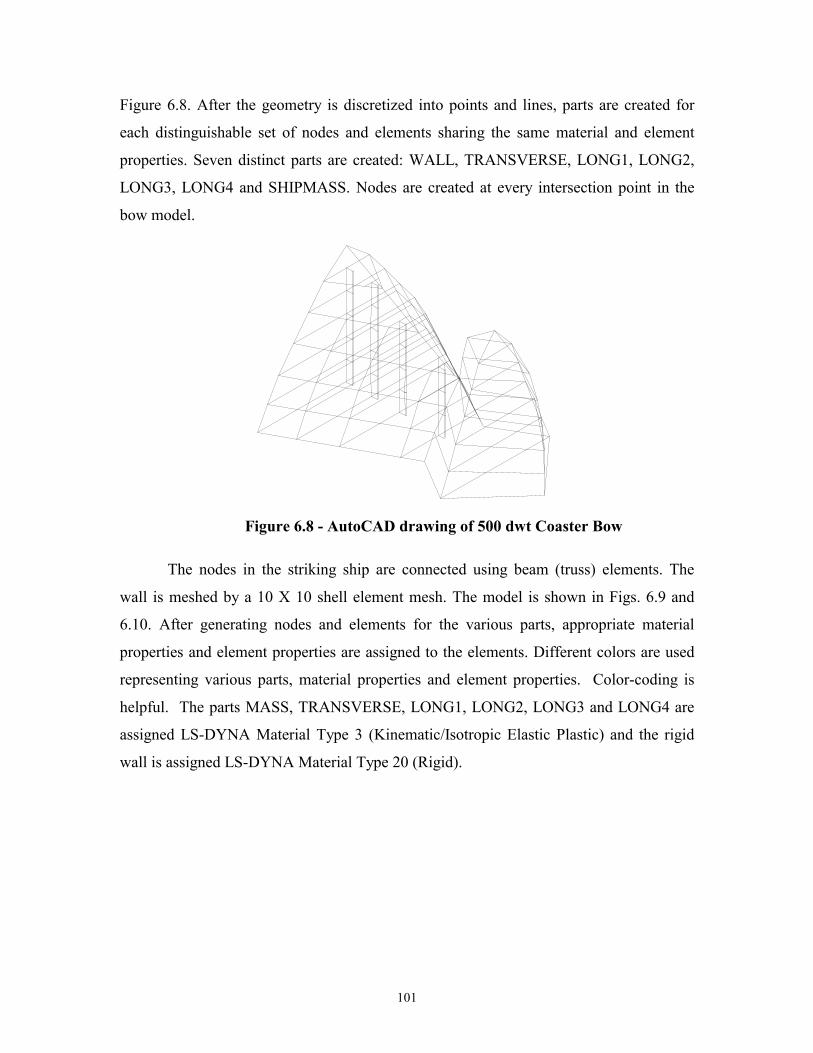
101
Figure 6.8. After the geometry is discretized into points and lines, parts are created for
each distinguishable set of nodes and elements sharing the same material and element
properties. Seven distinct parts are created: WALL, TRANSVERSE, LONG1, LONG2,
LONG3, LONG4 and SHIPMASS. Nodes are created at every intersection point in the
bow model.
Figure 6.8 - AutoCAD drawing of 500 dwt Coaster Bow
The nodes in the striking ship are connected using beam (truss) elements. The
wall is meshed by a 10 X 10 shell element mesh. The model is shown in Figs. 6.9 and
6.10. After generating nodes and elements for the various parts, appropriate material
properties and element properties are assigned to the elements. Different colors are used
representing various parts, material properties and element properties. Color-coding is
helpful. The parts MASS, TRANSVERSE, LONG1, LONG2, LONG3 and LONG4 are
assigned LS-DYNA Material Type 3 (Kinematic/Isotropic Elastic Plastic) and the rigid
wall is assigned LS-DYNA Material Type 20 (Rigid).
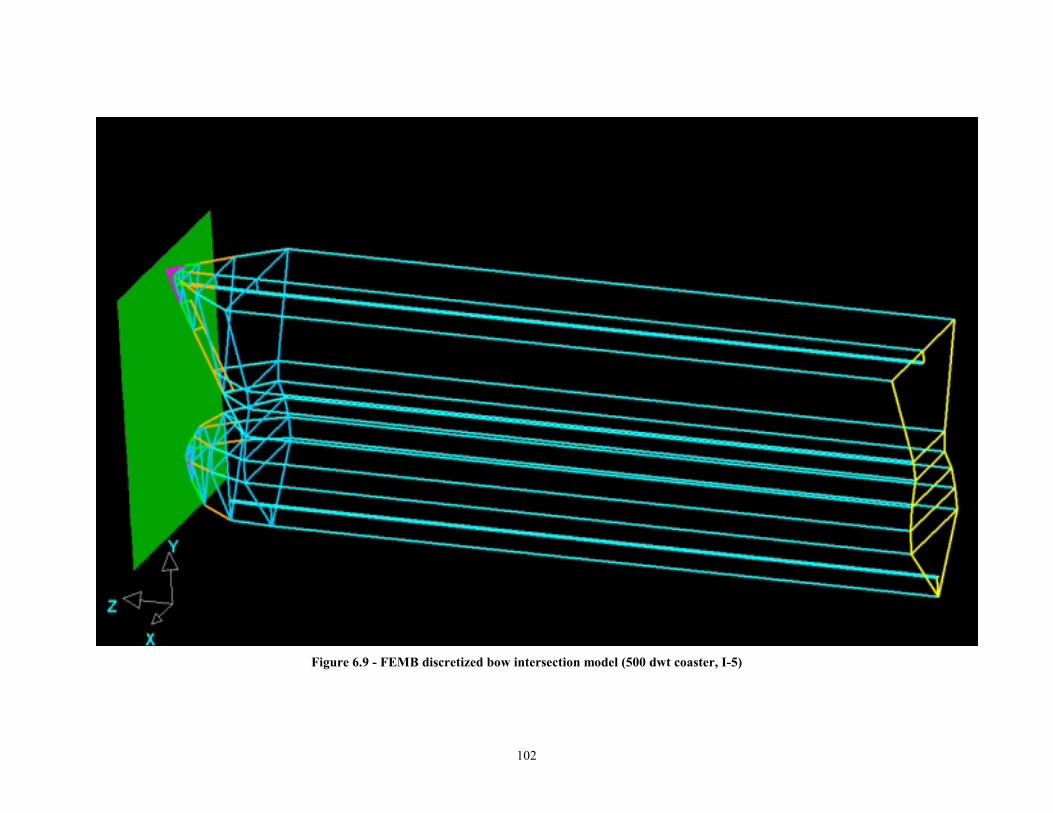
102
Figure 6.9 - FEMB discretized bow intersection model (500 dwt coaster, I-5)
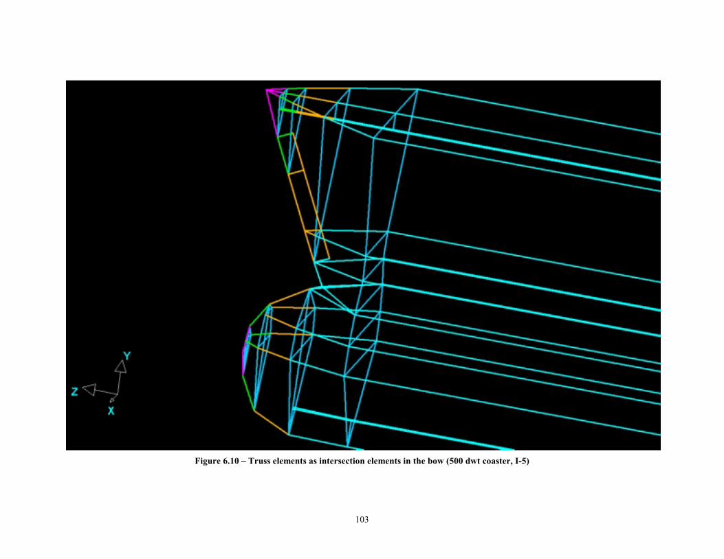
103
Figure 6.10 – Truss elements as intersection elements in the bow (500 dwt coaster, I-5)
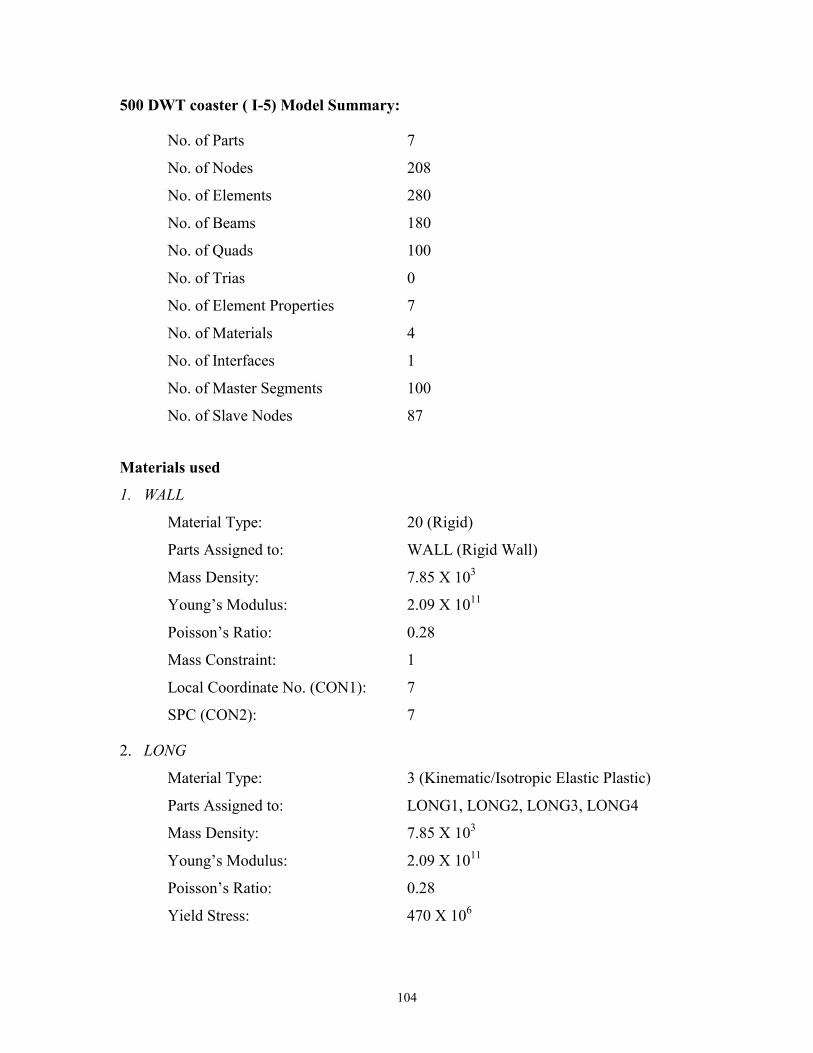
104
500 DWT coaster ( I-5) Model Summary:
No. of Parts 7
No. of Nodes 208
No. of Elements 280
No. of Beams 180
No. of Quads 100
No. of Trias 0
No. of Element Properties 7
No. of Materials 4
No. of Interfaces 1
No. of Master Segments 100
No. of Slave Nodes 87
Materials used
1. WALL
Material Type: 20 (Rigid)
Parts Assigned to: WALL (Rigid Wall)
Mass Density: 7.85 X 10³
Young’s Modulus: 2.09 X 10¹¹
Poisson’s Ratio: 0.28
Mass Constraint: 1
Local Coordinate No. (CON1): 7
SPC (CON2): 7
2. LONG
Material Type: 3 (Kinematic/Isotropic Elastic Plastic)
Parts Assigned to: LONG1, LONG2, LONG3, LONG4
Mass Density: 7.85 X 10³
Young’s Modulus: 2.09 X 10¹¹
Poisson’s Ratio: 0.28
Yield Stress: 470 X 106
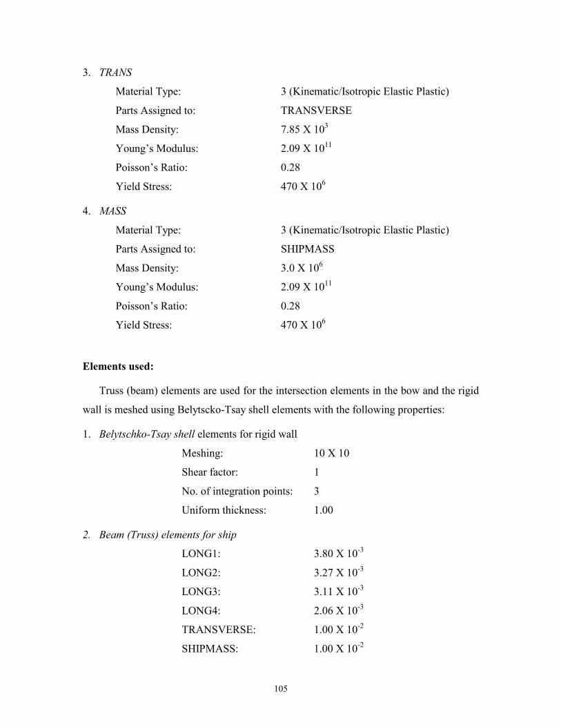
105
3. TRANS
Material Type: 3 (Kinematic/Isotropic Elastic Plastic)
Parts Assigned to: TRANSVERSE
Mass Density: 7.85 X 10³
Young’s Modulus: 2.09 X 10¹¹
Poisson’s Ratio: 0.28
Yield Stress: 470 X 106
4. MASS
Material Type: 3 (Kinematic/Isotropic Elastic Plastic)
Parts Assigned to: SHIPMASS
Mass Density: 3.0 X 10⁶
Young’s Modulus: 2.09 X 10¹¹
Poisson’s Ratio: 0.28
Yield Stress: 470 X 106
Elements used:
Truss (beam) elements are used for the intersection elements in the bow and the rigid
wall is meshed using Belytscko-Tsay shell elements with the following properties:
1. Belytschko-Tsay shell elements for rigid wall
Meshing: 10 X 10
Shear factor: 1
No. of integration points: 3
Uniform thickness: 1.00
2. Beam (Truss) elements for ship
LONG1: 3.80 X 10⁻³
LONG2: 3.27 X 10⁻³
LONG3: 3.11 X 10⁻³
LONG4: 2.06 X 10⁻³
TRANSVERSE: 1.00 X 10⁻²
SHIPMASS: 1.00 X 10⁻²

106
All nodes in the striking ship are assigned an initial velocity (see Figure 6.13)
equaling 5ms-1 in the first simulation and 12m/s in the second. Simulation is performed
on the model database file generated by FEMB after translating it into a .DYN file that is
executable by LS-DYNA.
107
Figure 6.11 – Contact Definition Showing Master Segments in Rigid Wall and Slave Nodes in the Bow (500 dwt coaster, I-5)
108
Figure 6.12 – Boundary Conditions on the Bow Model allow motion only in the direction of collision (500 dwt coaster, I-5)
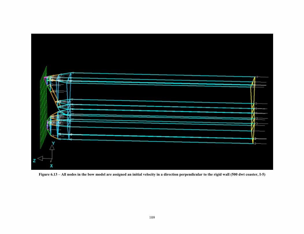
109
Figure 6.13 – All nodes in the bow model are assigned an initial velocity in a direction perpendicular to the rigid wall (500 dwt coaster, I-5)
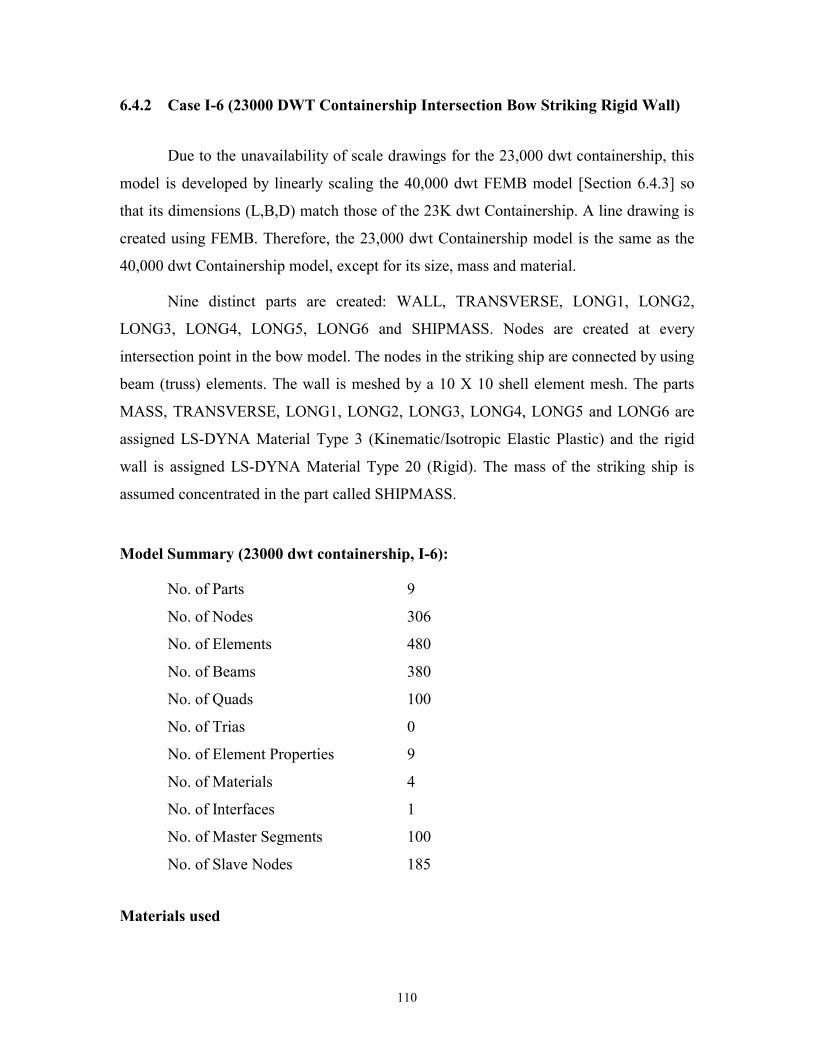
110
6.4.2 Case I-6 (23000 DWT Containership Intersection Bow Striking Rigid Wall)
Due to the unavailability of scale drawings for the 23,000 dwt containership, this
model is developed by linearly scaling the 40,000 dwt FEMB model [Section 6.4.3] so
that its dimensions (L,B,D) match those of the 23K dwt Containership. A line drawing is
created using FEMB. Therefore, the 23,000 dwt Containership model is the same as the
40,000 dwt Containership model, except for its size, mass and material.
Nine distinct parts are created: WALL, TRANSVERSE, LONG1, LONG2,
LONG3, LONG4, LONG5, LONG6 and SHIPMASS. Nodes are created at every
intersection point in the bow model. The nodes in the striking ship are connected by using
beam (truss) elements. The wall is meshed by a 10 X 10 shell element mesh. The parts
MASS, TRANSVERSE, LONG1, LONG2, LONG3, LONG4, LONG5 and LONG6 are
assigned LS-DYNA Material Type 3 (Kinematic/Isotropic Elastic Plastic) and the rigid
wall is assigned LS-DYNA Material Type 20 (Rigid). The mass of the striking ship is
assumed concentrated in the part called SHIPMASS.
Model Summary (23000 dwt containership, I-6):
No. of Parts 9
No. of Nodes 306
No. of Elements 480
No. of Beams 380
No. of Quads 100
No. of Trias 0
No. of Element Properties 9
No. of Materials 4
No. of Interfaces 1
No. of Master Segments 100
No. of Slave Nodes 185
Materials used
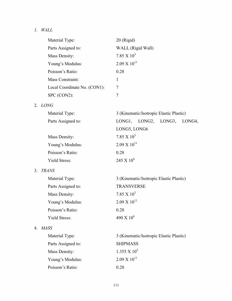
111
1. WALL
Material Type: 20 (Rigid)
Parts Assigned to: WALL (Rigid Wall)
Mass Density: 7.85 X 10³
Young’s Modulus: 2.09 X 10¹¹
Poisson’s Ratio: 0.28
Mass Constraint: 1
Local Coordinate No. (CON1): 7
SPC (CON2): 7
2. LONG
Material Type: 3 (Kinematic/Isotropic Elastic Plastic)
Parts Assigned to: LONG1, LONG2, LONG3, LONG4,
LONG5, LONG6
Mass Density: 7.85 X 10³
Young’s Modulus: 2.09 X 10¹¹
Poisson’s Ratio: 0.28
Yield Stress: 245 X 106
3. TRANS
Material Type: 3 (Kinematic/Isotropic Elastic Plastic)
Parts Assigned to: TRANSVERSE
Mass Density: 7.85 X 10³
Young’s Modulus: 2.09 X 10¹¹
Poisson’s Ratio: 0.28
Yield Stress: 490 X 106
4. MASS
Material Type: 3 (Kinematic/Isotropic Elastic Plastic)
Parts Assigned to: SHIPMASS
Mass Density: 1.355 X 10⁵
Young’s Modulus: 2.09 X 10¹¹
Poisson’s Ratio: 0.28
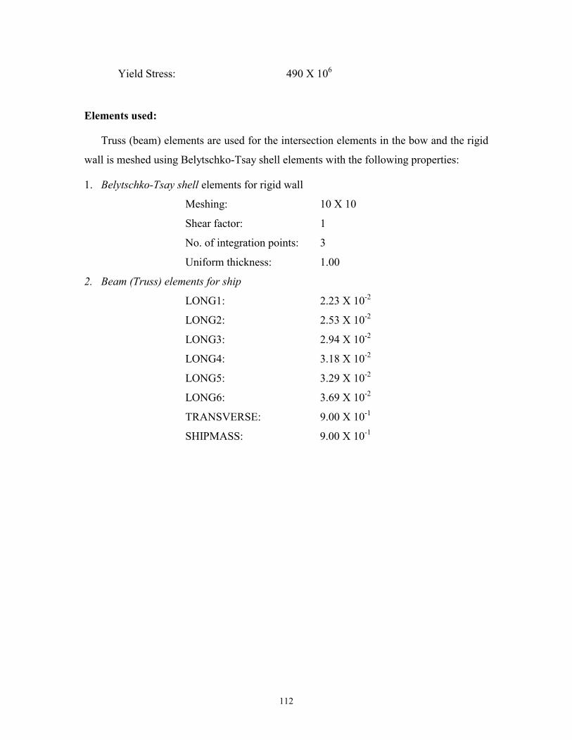
112
Yield Stress: 490 X 106
Elements used:
Truss (beam) elements are used for the intersection elements in the bow and the rigid
wall is meshed using Belytschko-Tsay shell elements with the following properties:
1. Belytschko-Tsay shell elements for rigid wall
Meshing: 10 X 10
Shear factor: 1
No. of integration points: 3
Uniform thickness: 1.00
2. Beam (Truss) elements for ship
LONG1: 2.23 X 10⁻²
LONG2: 2.53 X 10⁻²
LONG3: 2.94 X 10⁻²
LONG4: 3.18 X 10⁻²
LONG5: 3.29 X 10⁻²
LONG6: 3.69 X 10⁻²
TRANSVERSE: 9.00 X 10⁻¹
SHIPMASS: 9.00 X 10⁻¹
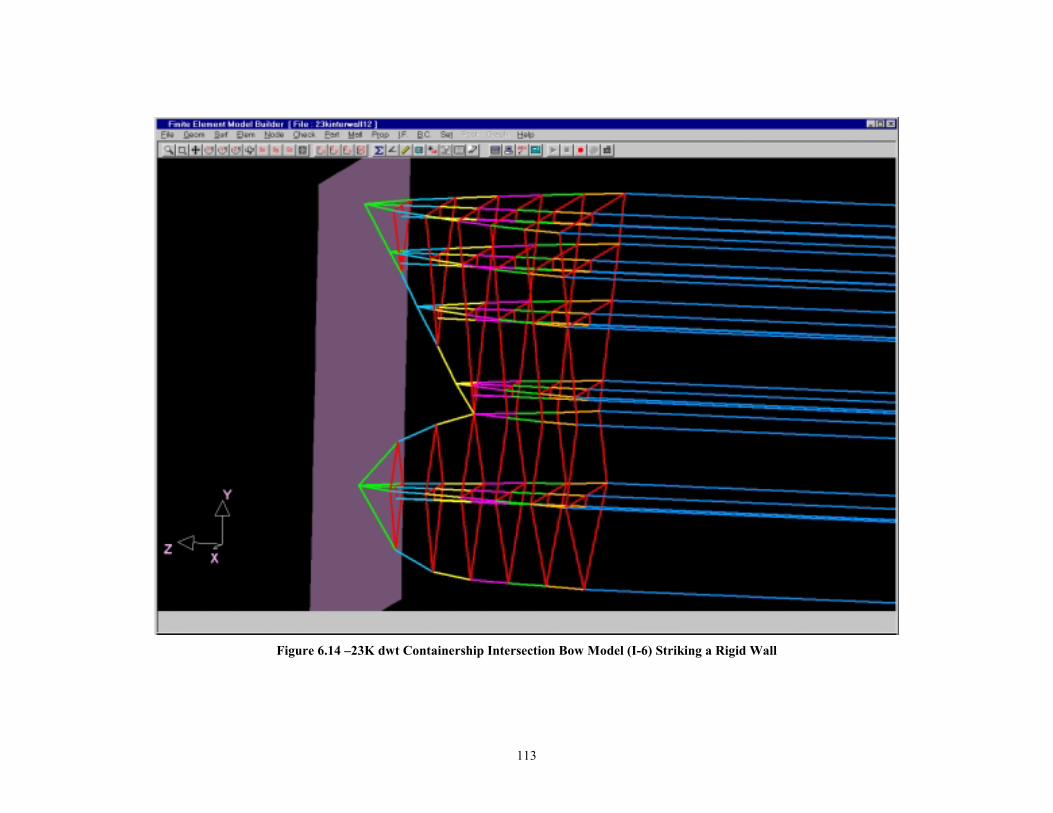
113
Figure 6.14 –23K dwt Containership Intersection Bow Model (I-6) Striking a Rigid Wall

114
6.4.3 Case I-7 (40000 DWT Containership Intersection Bow Striking Rigid Wall)
The initial line drawing is created using the Geometry Builder features of FEMB.
Nine distinct parts are created: WALL, TRANSVERSE, LONG1, LONG2, LONG3,
LONG4, LONG5, LONG6 and SHIPMASS. The parts MASS, TRANSVERSE, LONG1,
LONG2, LONG3, LONG4, LONG5 and LONG6 are assigned LS-DYNA Material Type
3 (Kinematic/Isotropic Elastic Plastic) and the rigid wall is assigned LS-DYNA Material
Type 20 (Rigid). The mass of the striking ship is assumed concentrated in the part called
SHIPMASS.
Model Summary:
No. of Parts 9
No. of Nodes 306
No. of Elements 480
No. of Beams 380
No. of Quads 100
No. of Trias 0
No. of Element Properties 9
No. of Materials 4
No. of Interfaces 1
No. of Master Segments 100
No. of Slave Nodes 185
Materials used
1. WALL
Material Type: 20 (Rigid)
Parts Assigned to: WALL (Rigid Wall)
Mass Density: 7.85 X 10³
Young’s Modulus: 2.09 X 10¹¹
Poisson’s Ratio: 0.28
Mass Constraint: 1

115
Local Coordinate No. (CON1): 7
SPC (CON2): 7
2. LONG
Material Type: 3 (Kinematic/Isotropic Elastic Plastic)
Parts Assigned to: LONG1, LONG2, LONG3, LONG4,
LONG5, LONG6.
Mass Density: 7.85 X 10³
Young’s Modulus: 2.09 X 10¹¹
Poisson’s Ratio: 0.28
Yield Stress: 340.7 X 10⁶
3. TRANS
Material Type: 3 (Kinematic/Isotropic Elastic Plastic)
Parts Assigned to: TRANSVERSE
Mass Density: 7.85 X 10³
Young’s Modulus: 2.09 X 10¹¹
Poisson’s Ratio: 0.28
Yield Stress: 340.1 X 10⁶
4. MASS
Material Type: 3 (Kinematic/Isotropic Elastic Plastic)
Parts Assigned to: SHIPMASS
Mass Density: 3.9 X 10⁵
Young’s Modulus: 2.09 X 10¹¹
Poisson’s Ratio: 0.28
Yield Stress: 340.7 X 10⁶
Elements used:
Truss (beam) elements are used for the intersection elements in the bow and the rigid
wall is meshed using Belytschko-Tsay shell elements with the following properties:
1. Belytschko-Tsay shell elements for rigid wall
Meshing: 10 X 10
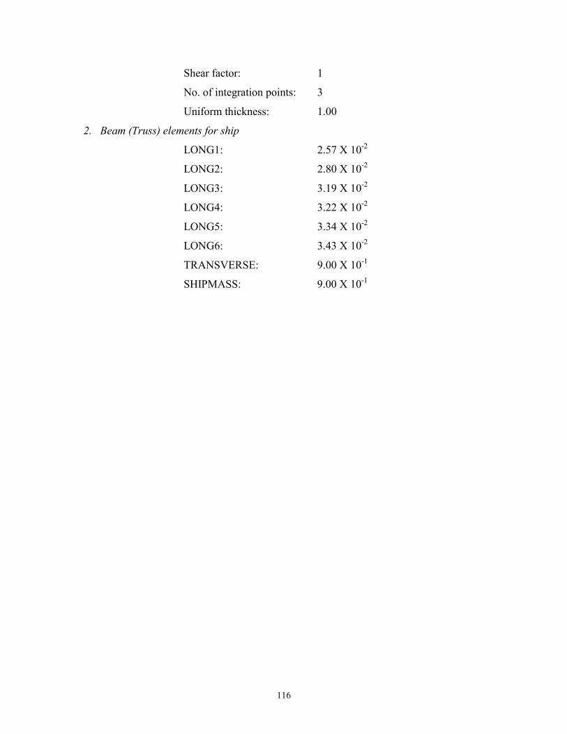
116
Shear factor: 1
No. of integration points: 3
Uniform thickness: 1.00
2. Beam (Truss) elements for ship
LONG1: 2.57 X 10⁻²
LONG2: 2.80 X 10⁻²
LONG3: 3.19 X 10⁻²
LONG4: 3.22 X 10⁻²
LONG5: 3.34 X 10⁻²
LONG6: 3.43 X 10⁻²
TRANSVERSE: 9.00 X 10⁻¹
SHIPMASS: 9.00 X 10⁻¹
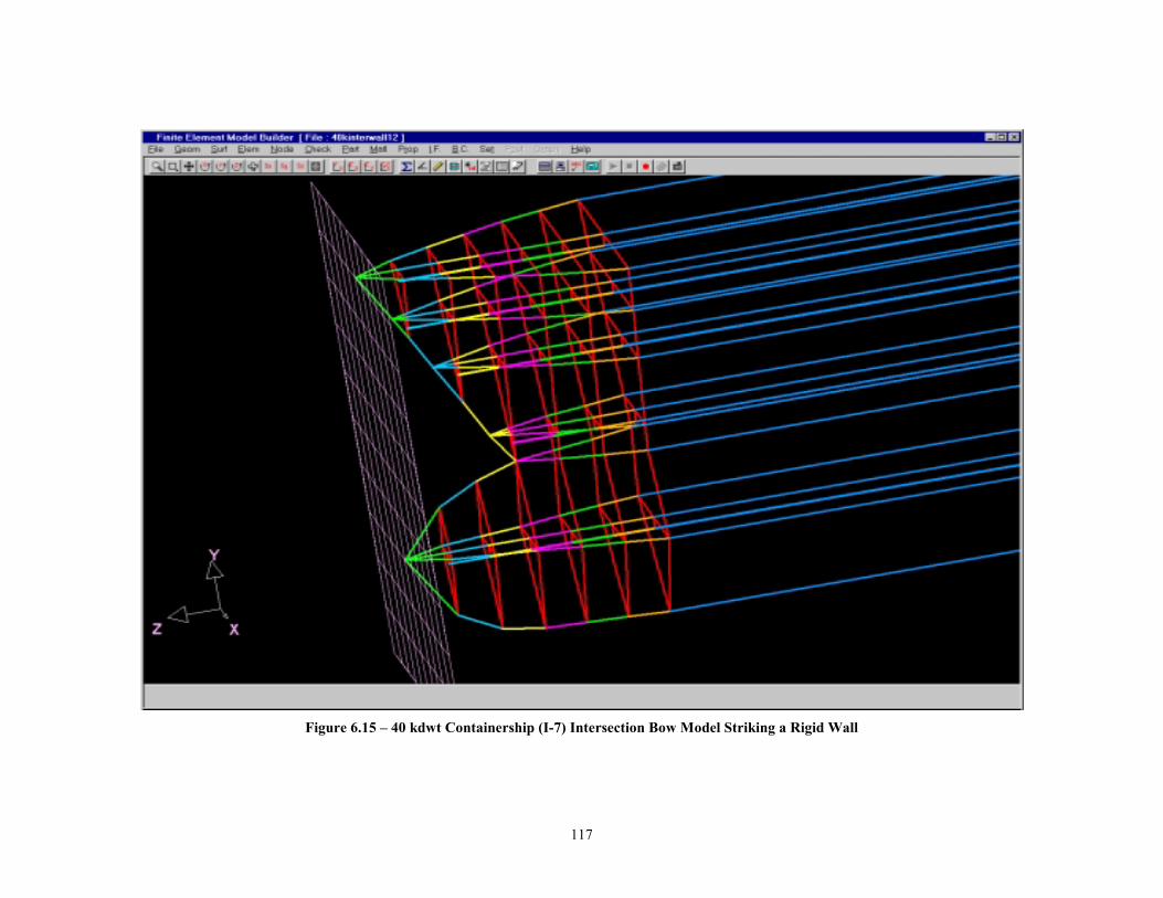
117
Figure 6.15 – 40 kdwt Containership (I-7) Intersection Bow Model Striking a Rigid Wall
118
6.4.4 Case I-8 (150000 DWT Bulk Carrier Intersection Bow Striking Rigid Wall)
The initial line drawing is created in FEMB. Nine distinct parts are created,
namely: WALL, TRANSVERSE, LONG1, LONG2, LONG3, LONG4, LONG5, LONG6
and SHIPMASS. The parts MASS, TRANSVERSE, LONG1, LONG2, LONG3,
LONG4, LONG5 and LONG6 are assigned LS-DYNA Material Type 3
(Kinematic/Isotropic Elastic Plastic) and the rigid wall is assigned LS-DYNA Material
Type 20 (Rigid). The mass of the striking ship is assumed concentrated in the part called
SHIPMASS.
Model Summary:
No. of Parts 9
No. of Nodes 228
No. of Elements 318
No. of Beams 218
No. of Quads 100
No. of Trias 0
No. of Element Properties 9
No. of Materials 4
No. of Interfaces 1
No. of Master Segments 100
No. of Slave Nodes 107
Materials used
1. WALL
Material Type: 20 (Rigid)
Parts Assigned to: WALL (Rigid Wall)
Mass Density: 7.85 X 10³
Young’s Modulus: 2.09 X 10¹¹
Poisson’s Ratio: 0.28
Mass Constraint: 1
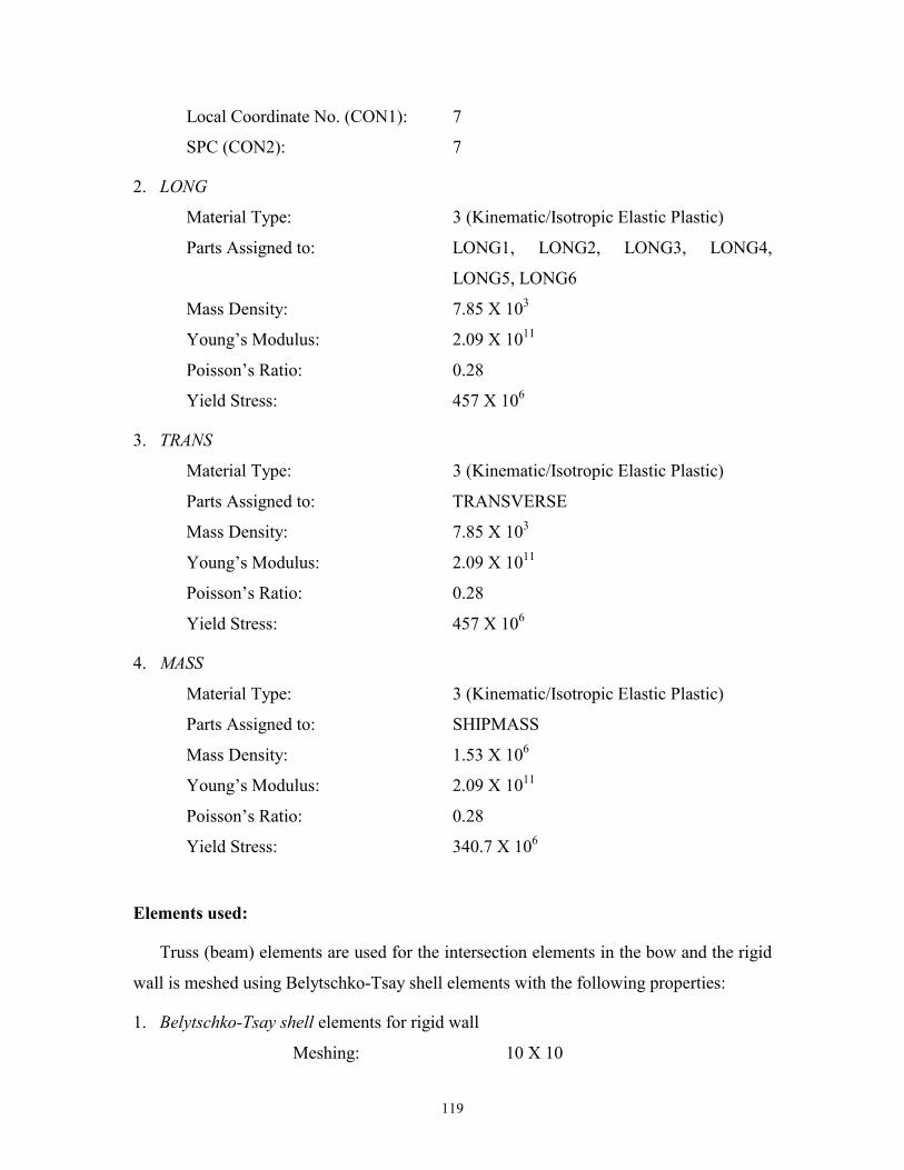
119
Local Coordinate No. (CON1): 7
SPC (CON2): 7
2. LONG
Material Type: 3 (Kinematic/Isotropic Elastic Plastic)
Parts Assigned to: LONG1, LONG2, LONG3, LONG4,
LONG5, LONG6
Mass Density: 7.85 X 10³
Young’s Modulus: 2.09 X 10¹¹
Poisson’s Ratio: 0.28
Yield Stress: 457 X 106
3. TRANS
Material Type: 3 (Kinematic/Isotropic Elastic Plastic)
Parts Assigned to: TRANSVERSE
Mass Density: 7.85 X 10³
Young’s Modulus: 2.09 X 10¹¹
Poisson’s Ratio: 0.28
Yield Stress: 457 X 106
4. MASS
Material Type: 3 (Kinematic/Isotropic Elastic Plastic)
Parts Assigned to: SHIPMASS
Mass Density: 1.53 X 10⁶
Young’s Modulus: 2.09 X 10¹¹
Poisson’s Ratio: 0.28
Yield Stress: 340.7 X 10⁶
Elements used:
Truss (beam) elements are used for the intersection elements in the bow and the rigid
wall is meshed using Belytschko-Tsay shell elements with the following properties:
1. Belytschko-Tsay shell elements for rigid wall
Meshing: 10 X 10
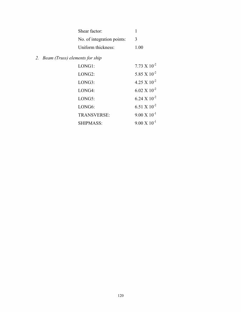
120
Shear factor: 1
No. of integration points: 3
Uniform thickness: 1.00
2. Beam (Truss) elements for ship
LONG1: 7.73 X 10⁻²
LONG2: 5.85 X 10⁻²
LONG3: 4.25 X 10⁻²
LONG4: 6.02 X 10⁻²
LONG5: 6.24 X 10⁻²
LONG6: 6.51 X 10⁻²
TRANSVERSE: 9.00 X 10⁻¹
SHIPMASS: 9.00 X 10⁻¹
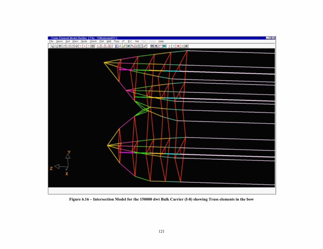
121
Figure 6.16 – Intersection Model for the 150000 dwt Bulk Carrier (I-8) showing Truss elements in the bow

122
6.5 Conventional Ship Side Models (Cases I-9, I-10, I-11 and I-12)
6.5.1 Cases I-9 and I-10 (23K DWT Intersection Containership Bow Striking
SH100 Conventional Side)
In these cases, the striking ship model is the 23K dwt intersection model
discussed in Section 6.4.2. A conventional model for the 100K dwt Single Hull struck
ship is created using FEMB. For simplicity and due to symmetry, only half (breadth-
wise) of the struck ship is modeled. Nine parts are created in the struck ship model:
STRKWEBS Webs
TRBULKHD Transverse Bulkheads
STRKSIDE Side Shell
STRKDK Decks
STRKBTM Bottom Plating
TANKWALL Tank Wall
STRKBILG Bilge Plating
STRKGUNW Gunwale Plating
STRKCL Plating along the CL of the ship
STRKSHIP Rest of the struck ship (mass distribution)
Model Summary:
No. of Parts 18 (9 in striking ship and 9 in struck ship)
No. of Nodes 1852
No. of Elements 2095
No. of Beams 444
No. of Quads 1509
No. of Trias 142
No. of Element Properties 15
No. of Materials 5
No. of Interfaces 1
No. of Master Segments 1609
No. of Slave Nodes 185
123
Materials used for the Struck Ship
1. STRKMASS
Material Type: 3 (Kinematic/Isotropic Elastic Plastic)
Parts Assigned to: STRKSHIP
Mass Density: 5.2 X 10⁵
Young’s Modulus: 2.09 X 10¹¹
Poisson’s Ratio: 0.28
Yield Stress: 315 X 106
2. STRK
Material Type: 3 (Kinematic/Isotropic Elastic Plastic)
Parts Assigned to: all other parts in the struck ship.
Mass Density: 7.85 X 10³
Young’s Modulus: 2.09 X 10¹¹
Poisson’s Ratio: 0.28
Yield Stress: 315 X 106
Truss (beam) elements are used for the intersection elements in the bow and the
struck ship is meshed using Belytschko-Tsay shell elements with different shell thickness
for each part, as defined in Table 6.2. Type 5 contact (NODES TO SURFACE) is
defined. All nodes in the striking ship are assigned as the slave nodes and all elements in
the struck ship are assigned as "Master Segments". Figure 6.17 shows the FE model of
the conventional 100K SH Tanker. The motion of the bow has been restricted to the
direction perpendicular to the undeformed outer shell of the struck ship. In case I-9, all
nodes on the centerline of the struck ship are fixed, and the rest of the nodes have only
one dof, in the direction of collision. In case I-10 (sway), all nodes have only the degree
of freedom in the direction of collision. Figure 6.18 shows a closer view of the
conventional struck ship model for the SH tanker.
Figures 6.19 and 6.20 show the collision between the 23 kdwt containership
intersection-bow and conventional SH100 tanker.
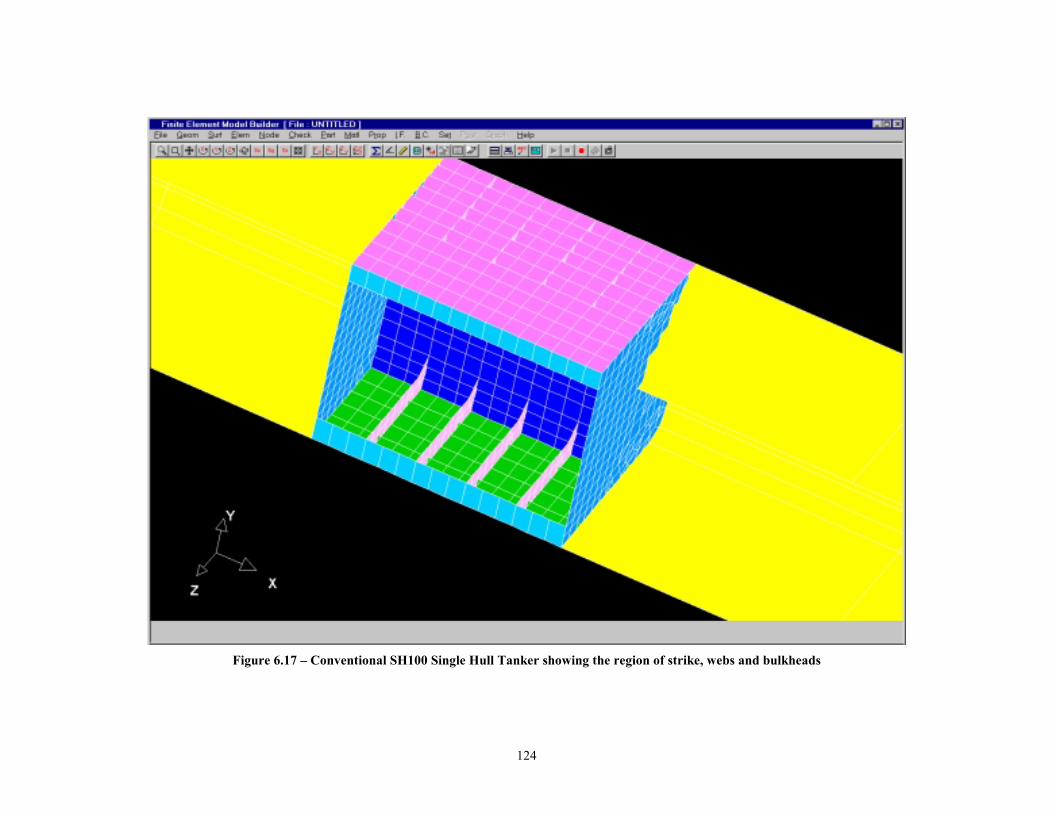
124
Figure 6.17 – Conventional SH100 Single Hull Tanker showing the region of strike, webs and bulkheads
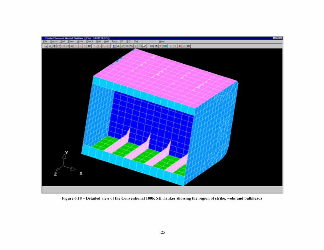
125
Figure 6.18 – Detailed view of the Conventional 100K SH Tanker showing the region of strike, webs and bulkheads
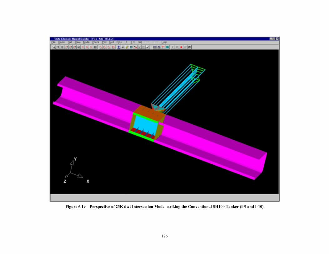
126
Figure 6.19 – Perspective of 23K dwt Intersection Model striking the Conventional SH100 Tanker (I-9 and I-10)
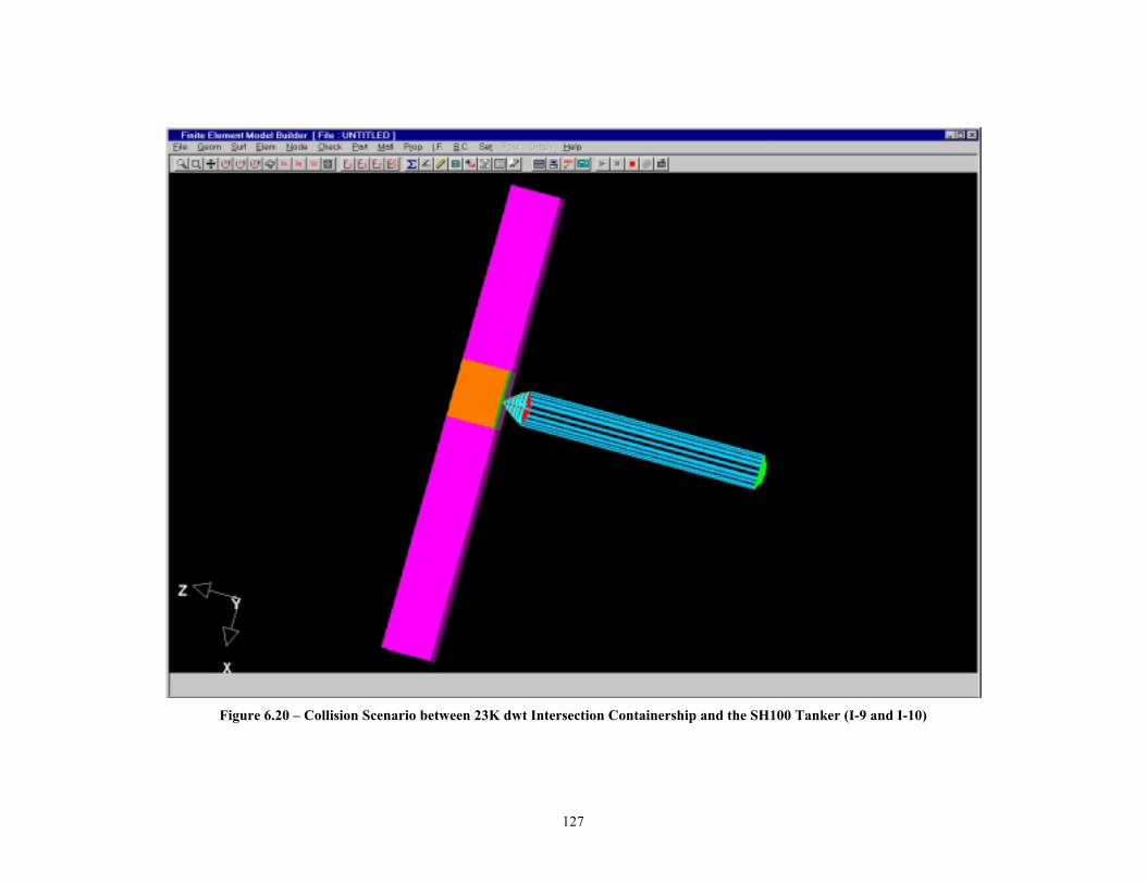
127
Figure 6.20 – Collision Scenario between 23K dwt Intersection Containership and the SH100 Tanker (I-9 and I-10)
128
6.5.2 Cases I-11 and I-12 (150K DWT Intersection Bulk Carrier Bow Striking
DH150 Conventional Side)
The striking ship model is the same as that of the 150 kdwt intersection model, as
discussed in Section 6.4.4. A conventional model for the 150 kdwt Double Hull tanker is
created using FEMB. For simplicity and due to symmetry, only half (breadth-wise) of
the struck ship is modeled. Nine parts are created in the struck ship model:
STRKWEBS Webs
TRBULKHD Transverse Bulkheads
STRKSIDE Side Shell
STRKDK Decks
STRKBTM Bottom Plating
TANKWALL Tank Wall
STRKGRDR Girders in the struck ship
DBLBTM Double Bottom Plating
DBLHULL Plating in the Double Hull
STRKSHIP Rest of the struck ship (mass distribution)
Model Summary:
No. of Parts 18 (9 in striking ship and 9 in struck ship)
No. of Nodes 1684
No. of Elements 2060
No. of Beams 132
No. of Quads 1868
No. of Trias 60
No. of Element Properties 15
No. of Materials 6
No. of Interfaces 1
No. of Master Segments 1932
No. of Slave Nodes 107
129
Materials used for the Struck Ship
1. STRKMASS
Material Type: 3 (Kinematic/Isotropic Elastic Plastic)
Parts Assigned to: STRKSHIP
Mass Density: 5.2 X 10⁵
Young’s Modulus: 2.09 X 10¹¹
Poisson’s Ratio: 0.28
Yield Stress: 315 X 106
2. STRK
Material Type: 3 (Kinematic/Isotropic Elastic Plastic)
Parts Assigned to: all other parts in the struck ship.
Mass Density: 7.85 X 10³
Young’s Modulus: 2.09 X 10¹¹
Poisson’s Ratio: 0.28
Yield Stress: 315 X 106
Truss (beam) elements are used for the intersection elements in the bow and the
struck ship is meshed using Belytschko-Tsay shell elements with different shell thickness
for each part, as defined in Table 6.2.
Type 5 contact (NODES TO SURFACE) is defined. All nodes in the striking ship
are assigned as the slave nodes and all elements in the struck ship are assigned as "Master
Segments". Figure 6.21 shows the FE model of the conventional 150K DH Tanker. The
motion of the bow is restricted to the direction perpendicular to the un-deformed outer
shell of the struck ship. In case I-11, all nodes on the centerline of the struck ship are
fixed, and the rest of the nodes have only one dof, in the direction of collision. In case I-
12 (sway), all nodes have only the degree of freedom in the direction of collision.
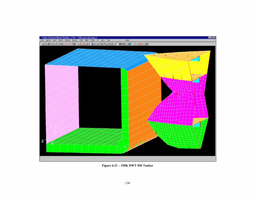
130
Figure 6.21 – 150K DWT DH Tanker
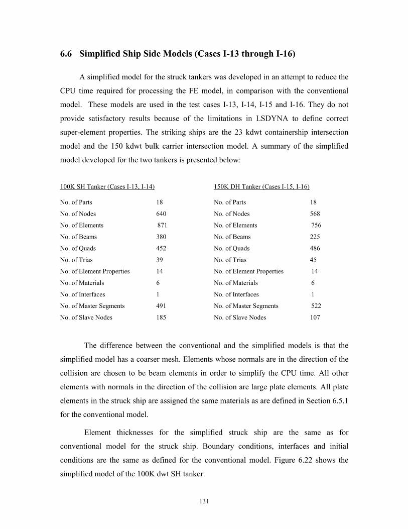
131
6.6 Simplified Ship Side Models (Cases I-13 through I-16)
A simplified model for the struck tankers was developed in an attempt to reduce the
CPU time required for processing the FE model, in comparison with the conventional
model. These models are used in the test cases I-13, I-14, I-15 and I-16. They do not
provide satisfactory results because of the limitations in LSDYNA to define correct
super-element properties. The striking ships are the 23 kdwt containership intersection
model and the 150 kdwt bulk carrier intersection model. A summary of the simplified
model developed for the two tankers is presented below:
100K SH Tanker (Cases I-13, I-14)
No. of Parts 18
No. of Nodes 640
No. of Elements 871
No. of Beams 380
No. of Quads 452
No. of Trias 39
No. of Element Properties 14
No. of Materials 6
No. of Interfaces 1
No. of Master Segments 491
No. of Slave Nodes 185
150K DH Tanker (Cases I-15, I-16)
No. of Parts 18
No. of Nodes 568
No. of Elements 756
No. of Beams 225
No. of Quads 486
No. of Trias 45
No. of Element Properties 14
No. of Materials 6
No. of Interfaces 1
No. of Master Segments 522
No. of Slave Nodes 107
The difference between the conventional and the simplified models is that the
simplified model has a coarser mesh. Elements whose normals are in the direction of the
collision are chosen to be beam elements in order to simplify the CPU time. All other
elements with normals in the direction of the collision are large plate elements. All plate
elements in the struck ship are assigned the same materials as are defined in Section 6.5.1
for the conventional model.
Element thicknesses for the simplified struck ship are the same as for
conventional model for the struck ship. Boundary conditions, interfaces and initial
conditions are the same as defined for the conventional model. Figure 6.22 shows the
simplified model of the 100K dwt SH tanker.
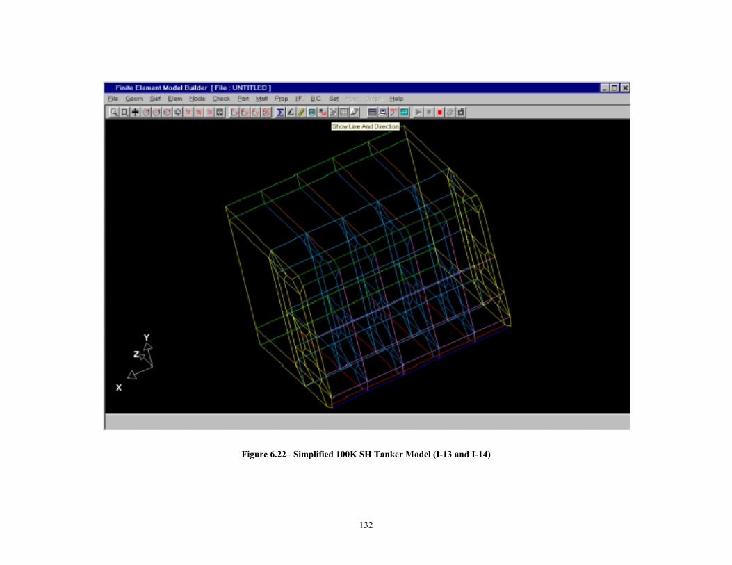
132
Figure 6.22– Simplified 100K SH Tanker Model (I-13 and I-14)
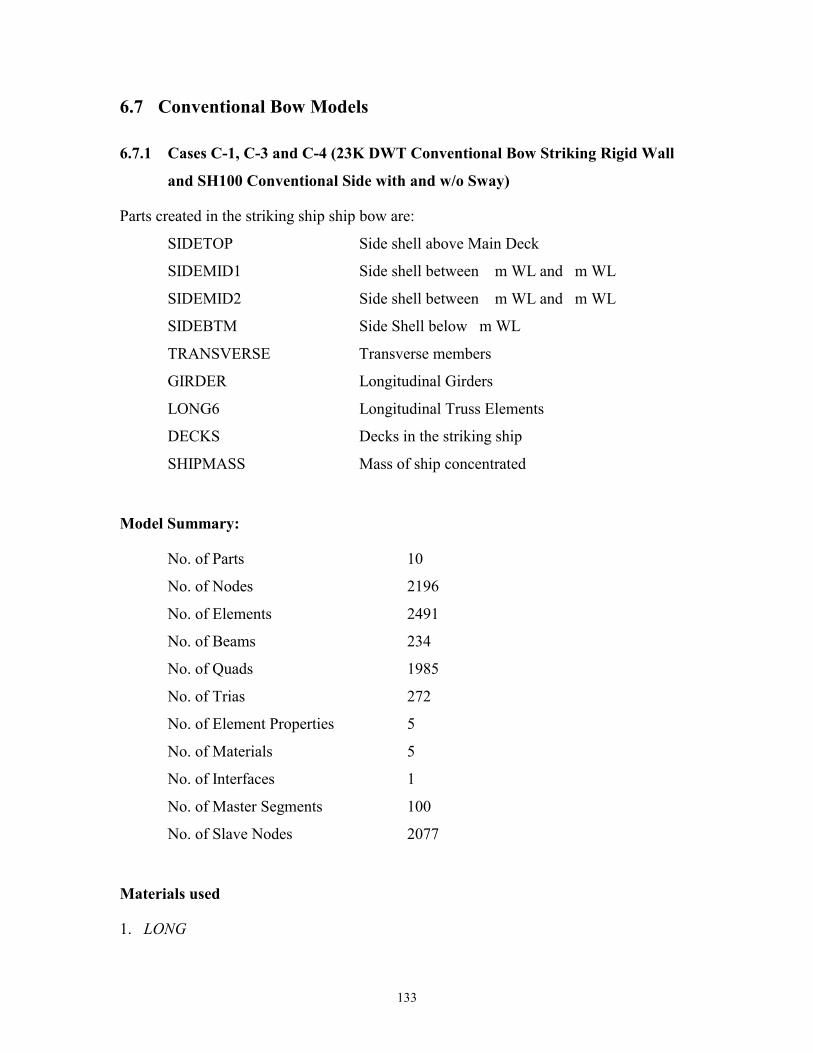
133
6.7 Conventional Bow Models
6.7.1 Cases C-1, C-3 and C-4 (23K DWT Conventional Bow Striking Rigid Wall
and SH100 Conventional Side with and w/o Sway)
Parts created in the striking ship ship bow are:
SIDETOP Side shell above Main Deck
SIDEMID1 Side shell between m WL and m WL
SIDEMID2 Side shell between m WL and m WL
SIDEBTM Side Shell below m WL
TRANSVERSE Transverse members
GIRDER Longitudinal Girders
LONG6 Longitudinal Truss Elements
DECKS Decks in the striking ship
SHIPMASS Mass of ship concentrated
Model Summary:
No. of Parts 10
No. of Nodes 2196
No. of Elements 2491
No. of Beams 234
No. of Quads 1985
No. of Trias 272
No. of Element Properties 5
No. of Materials 5
No. of Interfaces 1
No. of Master Segments 100
No. of Slave Nodes 2077
Materials used
1. LONG

134
Material Type: 3 (Kinematic/Isotropic Elastic Plastic)
Parts Assigned to: LONG6
Mass Density: 7.85 X 10³
Young’s Modulus: 2.09 X 10¹¹
Poisson’s Ratio: 0.28
Yield Stress: 235 X 106
2. TRANS
Material Type: 3 (Kinematic/Isotropic Elastic Plastic)
Parts Assigned to: TRANSVERSE
Mass Density: 7.85 X 10³
Young’s Modulus: 2.09 X 10¹¹
Poisson’s Ratio: 0.28
Yield Stress: 235 X 106
3. MASS
Material Type: 3 (Kinematic/Isotropic Elastic Plastic)
Parts Assigned to: SHIPMASS
Mass Density: 1.52 X 10⁵
Young’s Modulus: 2.09 X 10¹¹
Poisson’s Ratio: 0.28
Yield Stress: 235 X 106
4. SHELL
Material Type: 3 (Kinematic/Isotropic Elastic Plastic)
Parts Assigned to: Striking Ship Side Shell
Mass Density: 7.85 X 10³
Young’s Modulus: 2.09 X 10¹¹
Poisson’s Ratio: 0.28
Yield Stress: 235 X 106
Type 5 contact (NODES TO SURFACE) is defined. All nodes in the striking ship
are assigned as the slave nodes and all elements in the rigid-wall are assigned as "Master
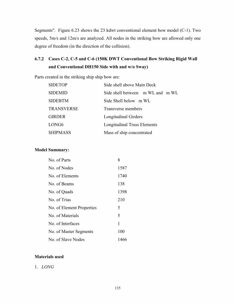
135
Segments". Figure 6.23 shows the 23 kdwt conventional element bow model (C-1). Two
speeds, 5m/s and 12m/s are analyzed. All nodes in the striking bow are allowed only one
degree of freedom (in the direction of the collision).
6.7.2 Cases C-2, C-5 and C-6 (150K DWT Conventional Bow Striking Rigid Wall
and Conventional DH150 Side with and w/o Sway)
Parts created in the striking ship ship bow are:
SIDETOP Side shell above Main Deck
SIDEMID Side shell between m WL and m WL
SIDEBTM Side Shell below m WL
TRANSVERSE Transverse members
GIRDER Longitudinal Girders
LONG6 Longitudinal Truss Elements
SHIPMASS Mass of ship concentrated
Model Summary:
No. of Parts 8
No. of Nodes 1587
No. of Elements 1740
No. of Beams 138
No. of Quads 1398
No. of Trias 210
No. of Element Properties 5
No. of Materials 5
No. of Interfaces 1
No. of Master Segments 100
No. of Slave Nodes 1466
Materials used
1. LONG
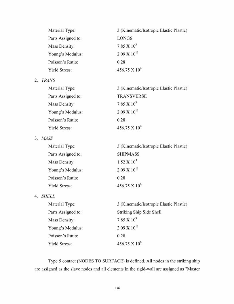
136
Material Type: 3 (Kinematic/Isotropic Elastic Plastic)
Parts Assigned to: LONG6
Mass Density: 7.85 X 10³
Young’s Modulus: 2.09 X 10¹¹
Poisson’s Ratio: 0.28
Yield Stress: 456.75 X 10⁶
2. TRANS
Material Type: 3 (Kinematic/Isotropic Elastic Plastic)
Parts Assigned to: TRANSVERSE
Mass Density: 7.85 X 10³
Young’s Modulus: 2.09 X 10¹¹
Poisson’s Ratio: 0.28
Yield Stress: 456.75 X 10⁶
3. MASS
Material Type: 3 (Kinematic/Isotropic Elastic Plastic)
Parts Assigned to: SHIPMASS
Mass Density: 1.52 X 10⁵
Young’s Modulus: 2.09 X 10¹¹
Poisson’s Ratio: 0.28
Yield Stress: 456.75 X 10⁶
4. SHELL
Material Type: 3 (Kinematic/Isotropic Elastic Plastic)
Parts Assigned to: Striking Ship Side Shell
Mass Density: 7.85 X 10³
Young’s Modulus: 2.09 X 10¹¹
Poisson’s Ratio: 0.28
Yield Stress: 456.75 X 10⁶
Type 5 contact (NODES TO SURFACE) is defined. All nodes in the striking ship
are assigned as the slave nodes and all elements in the rigid-wall are assigned as "Master

137
Segments". Figure 6.24 shows the 150 kdwt conventional element bow model (C-2).
Two speeds, 5m/s and 12m/s are analyzed. All nodes in the striking bow are allowed only
one degree of freedom (in the direction of the collision). Figures 6.25 and 6.26 show the
150 kdwt conventional bow model striking the DH150 and SH100 conventional side
models (C-3 and C-5). These models were described in Section 6.5.
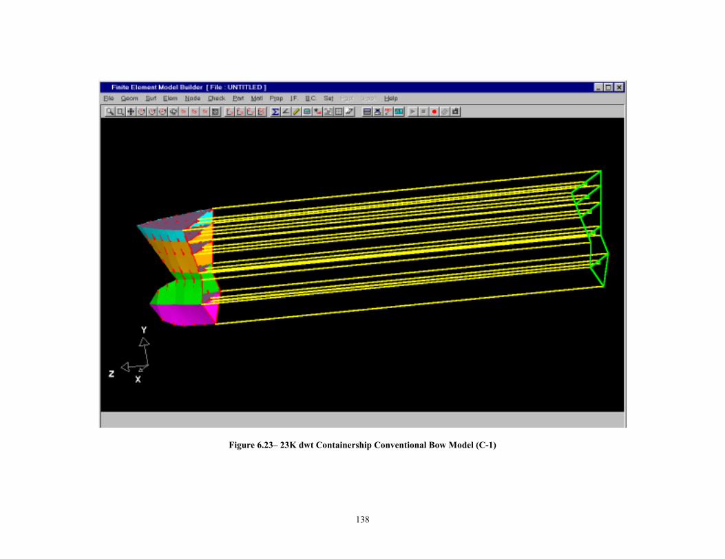
138
Figure 6.23– 23K dwt Containership Conventional Bow Model (C-1)
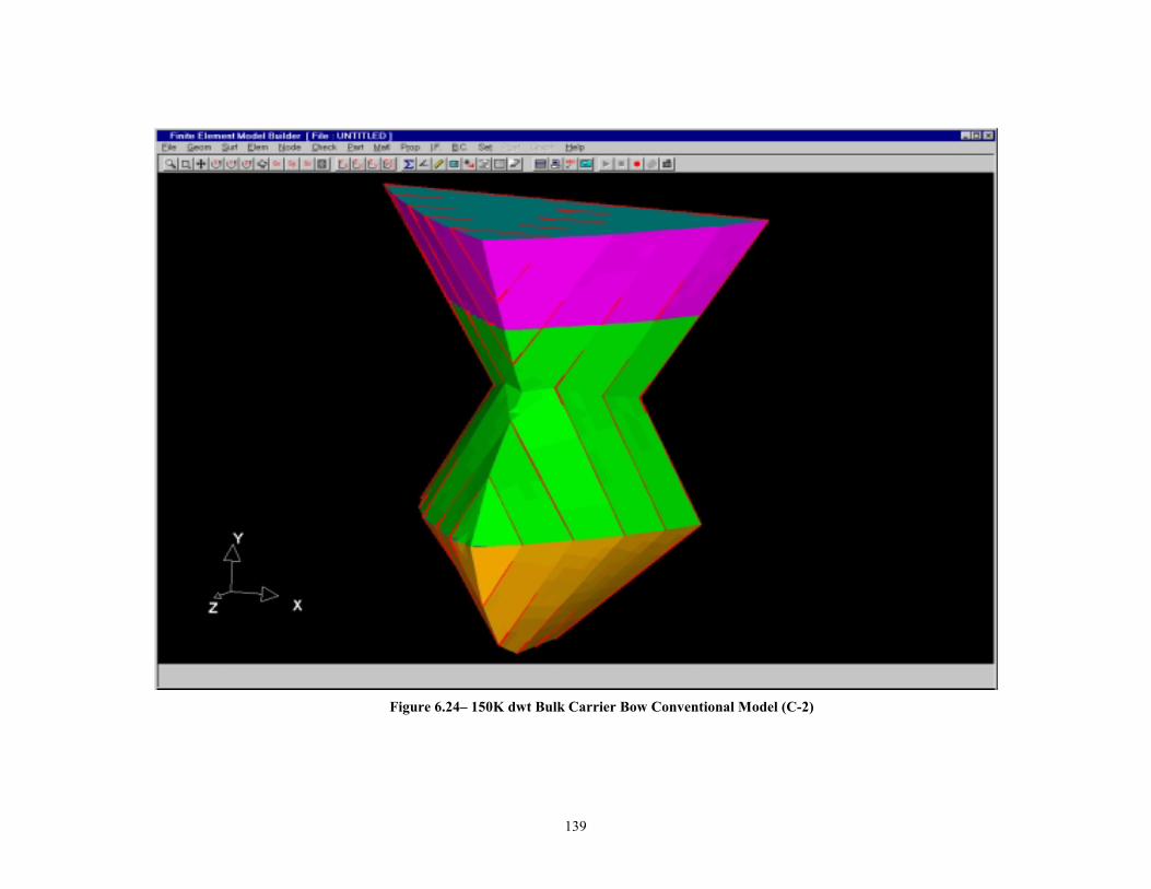
139
Figure 6.24– 150K dwt Bulk Carrier Bow Conventional Model (C-2)
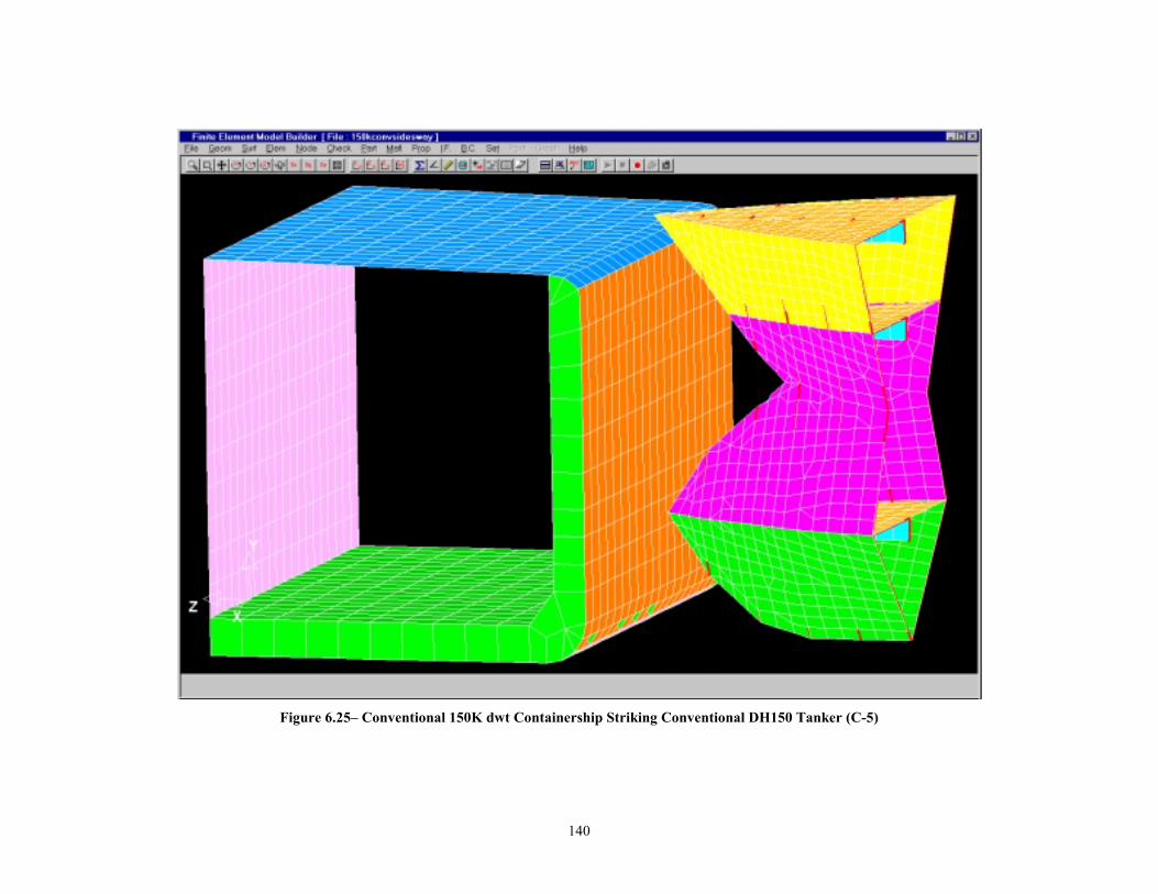
140
Figure 6.25– Conventional 150K dwt Containership Striking Conventional DH150 Tanker (C-5)
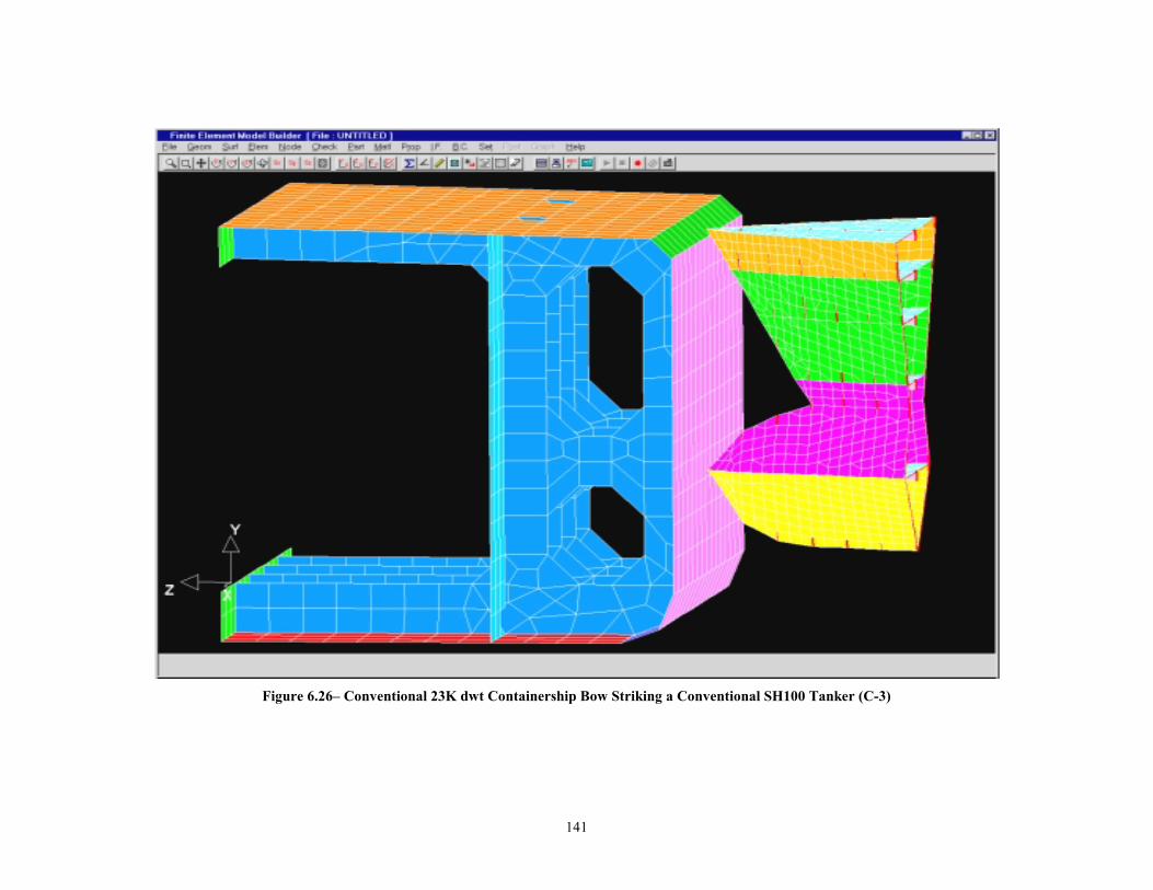
141
Figure 6.26– Conventional 23K dwt Containership Bow Striking a Conventional SH100 Tanker (C-3)
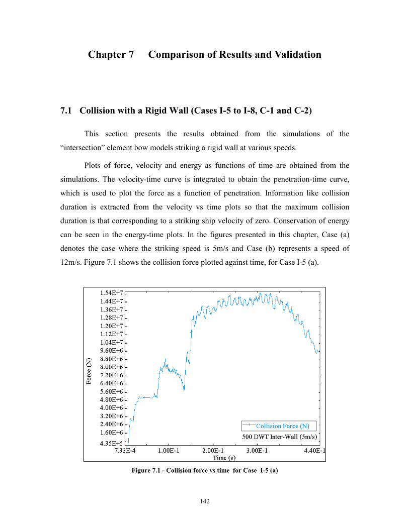
142
Chapter 7 Comparison of Results and Validation 7.1 Collision with a Rigid Wall (Cases I-5 to I-8, C-1 and C-2)
This section presents the results obtained from the simulations of the
“intersection” element bow models striking a rigid wall at various speeds.
Plots of force, velocity and energy as functions of time are obtained from the
simulations. The velocity-time curve is integrated to obtain the penetration-time curve,
which is used to plot the force as a function of penetration. Information like collision
duration is extracted from the velocity vs time plots so that the maximum collision
duration is that corresponding to a striking ship velocity of zero. Conservation of energy
can be seen in the energy-time plots. In the figures presented in this chapter, Case (a)
denotes the case where the striking speed is 5m/s and Case (b) represents a speed of
12m/s. Figure 7.1 shows the collision force plotted against time, for Case I-5 (a).
Figure 7.1 - Collision force vs time for Case I-5 (a)
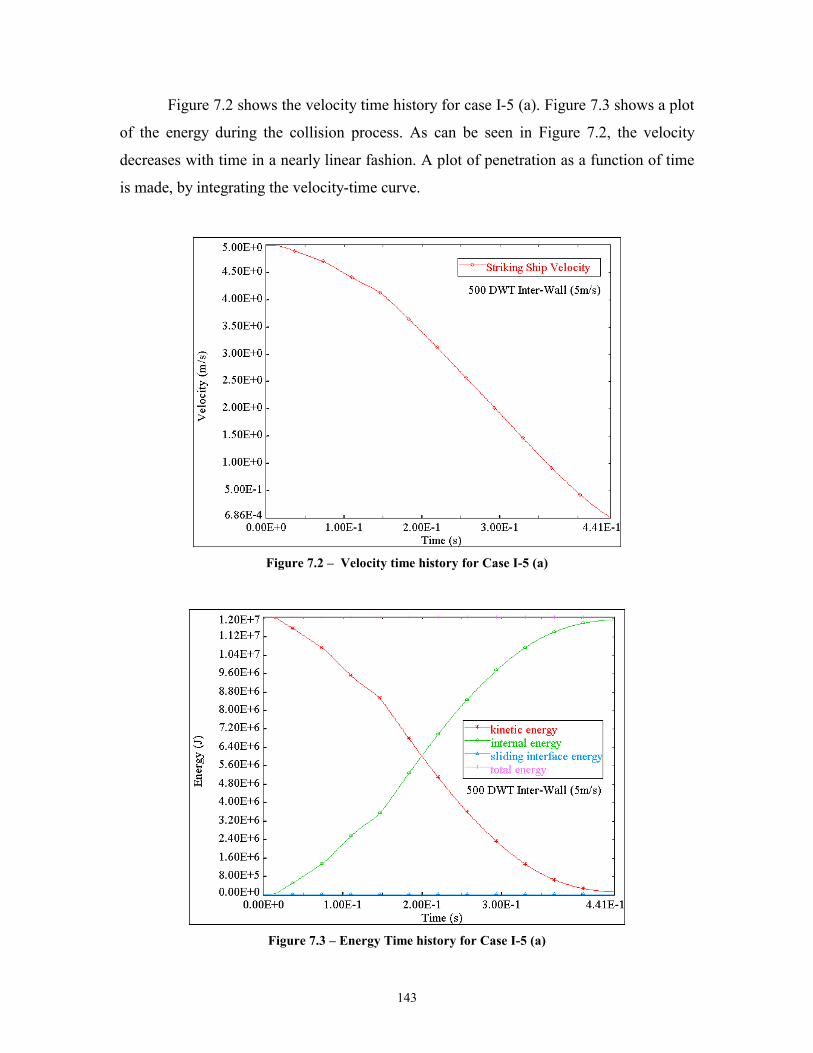
143
Figure 7.2 shows the velocity time history for case I-5 (a). Figure 7.3 shows a plot
of the energy during the collision process. As can be seen in Figure 7.2, the velocity
decreases with time in a nearly linear fashion. A plot of penetration as a function of time
is made, by integrating the velocity-time curve.
Figure 7.2 – Velocity time history for Case I-5 (a)
Figure 7.3 – Energy Time history for Case I-5 (a)
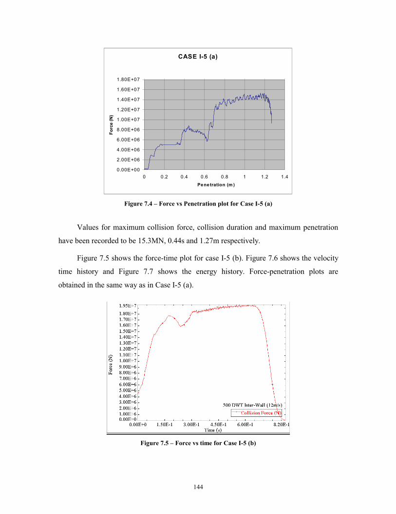
144
CASE I-5 (a)
0.00E+00
2.00E+06
4.00E+06
6.00E+06
8.00E+06
1.00E+07
1.20E+07
1.40E+07
1.60E+07
1.80E+07
0 0.2 0.4 0.6 0.8 1 1.2 1.4Penetration (m )
Forc
e (N
)
Figure 7.4 – Force vs Penetration plot for Case I-5 (a)
Values for maximum collision force, collision duration and maximum penetration
have been recorded to be 15.3MN, 0.44s and 1.27m respectively.
Figure 7.5 shows the force-time plot for case I-5 (b). Figure 7.6 shows the velocity
time history and Figure 7.7 shows the energy history. Force-penetration plots are
obtained in the same way as in Case I-5 (a).
Figure 7.5 – Force vs time for Case I-5 (b)
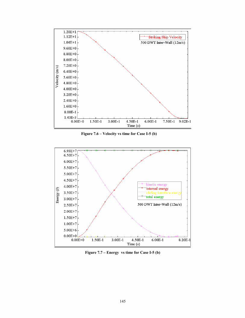
145
Figure 7.6 – Velocity vs time for Case I-5 (b)
Figure 7.7 – Energy vs time for Case I-5 (b)
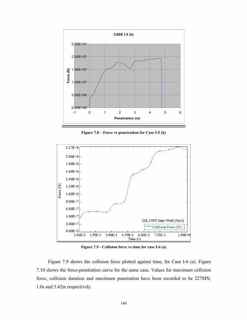
146
CASE I-5 (b)
0.00E+00
5.00E+06
1.00E+07
1.50E+07
2.00E+07
2.50E+07
-1 0 1 2 3 4 5 6
Penetration (m)
Forc
e (N
)
Figure 7.8 – Force vs penetration for Case I-5 (b)
Figure 7.9 - Collision force vs time for case I-6 (a)
Figure 7.9 shows the collision force plotted against time, for Case I-6 (a). Figure
7.10 shows the force-penetration curve for the same case. Values for maximum collision
force, collision duration and maximum penetration have been recorded to be 227MN,
1.0s and 3.42m respectively.
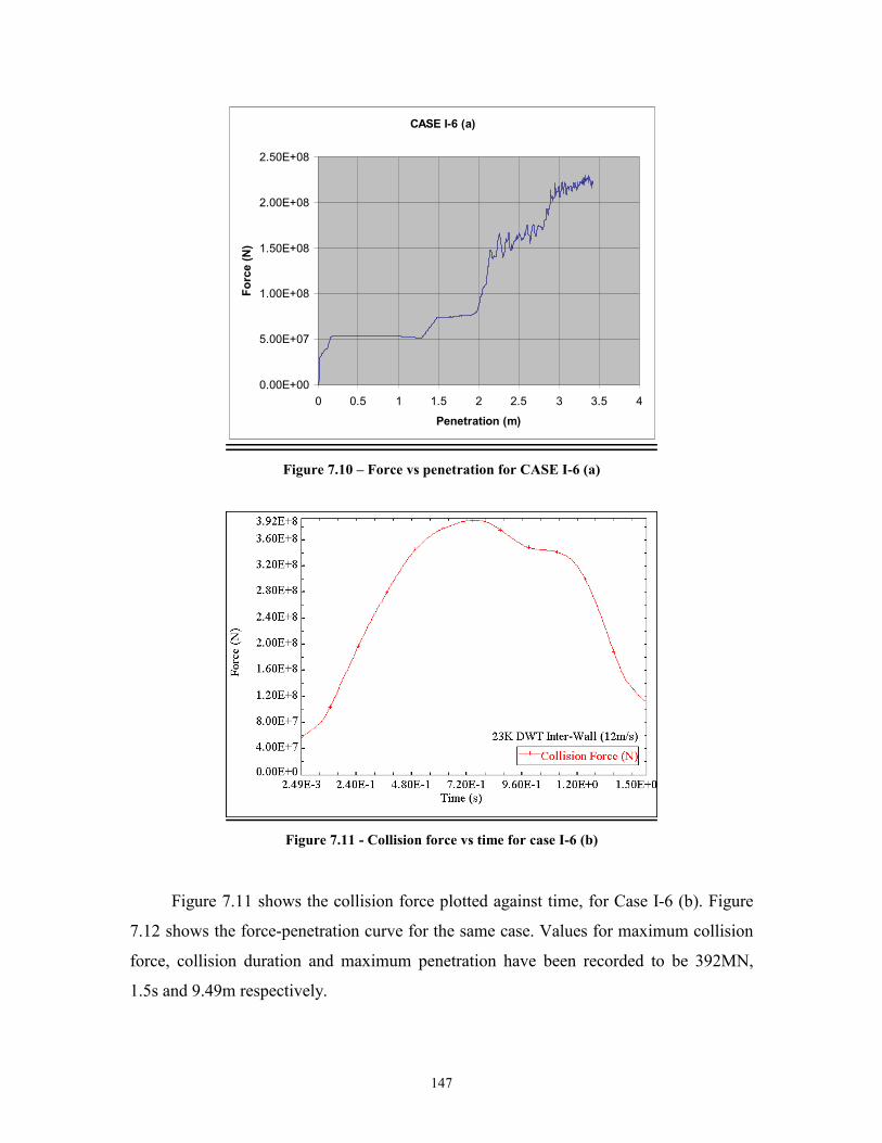
147
CASE I-6 (a)
0.00E+00
5.00E+07
1.00E+08
1.50E+08
2.00E+08
2.50E+08
0 0.5 1 1.5 2 2.5 3 3.5 4
Penetration (m)
Forc
e (N
)
Figure 7.10 – Force vs penetration for CASE I-6 (a)
Figure 7.11 - Collision force vs time for case I-6 (b)
Figure 7.11 shows the collision force plotted against time, for Case I-6 (b). Figure
7.12 shows the force-penetration curve for the same case. Values for maximum collision
force, collision duration and maximum penetration have been recorded to be 392MN,
1.5s and 9.49m respectively.
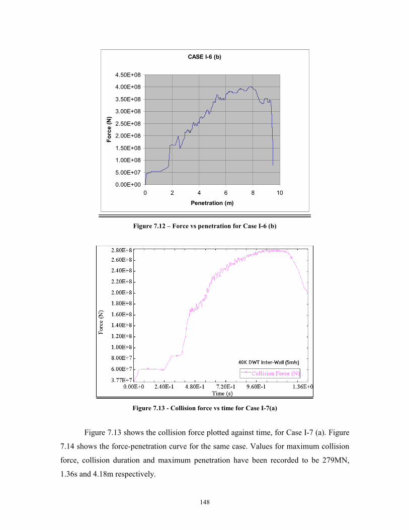
148
CASE I-6 (b)
0.00E+00
5.00E+07
1.00E+08
1.50E+08
2.00E+08
2.50E+08
3.00E+08
3.50E+08
4.00E+08
4.50E+08
0 2 4 6 8 10
Penetration (m)
Forc
e (N
)
Figure 7.12 – Force vs penetration for Case I-6 (b)
Figure 7.13 - Collision force vs time for Case I-7(a)
Figure 7.13 shows the collision force plotted against time, for Case I-7 (a). Figure
7.14 shows the force-penetration curve for the same case. Values for maximum collision
force, collision duration and maximum penetration have been recorded to be 279MN,
1.36s and 4.18m respectively.
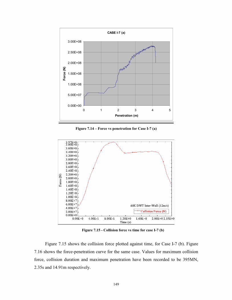
149
CASE I-7 (a)
0.00E+00
5.00E+07
1.00E+08
1.50E+08
2.00E+08
2.50E+08
3.00E+08
0 1 2 3 4 5
Penetration (m)
Forc
e (N
)
Figure 7.14 – Force vs penetration for Case I-7 (a)
Figure 7.15 - Collision force vs time for case I-7 (b)
Figure 7.15 shows the collision force plotted against time, for Case I-7 (b). Figure
7.16 shows the force-penetration curve for the same case. Values for maximum collision
force, collision duration and maximum penetration have been recorded to be 395MN,
2.35s and 14.91m respectively.
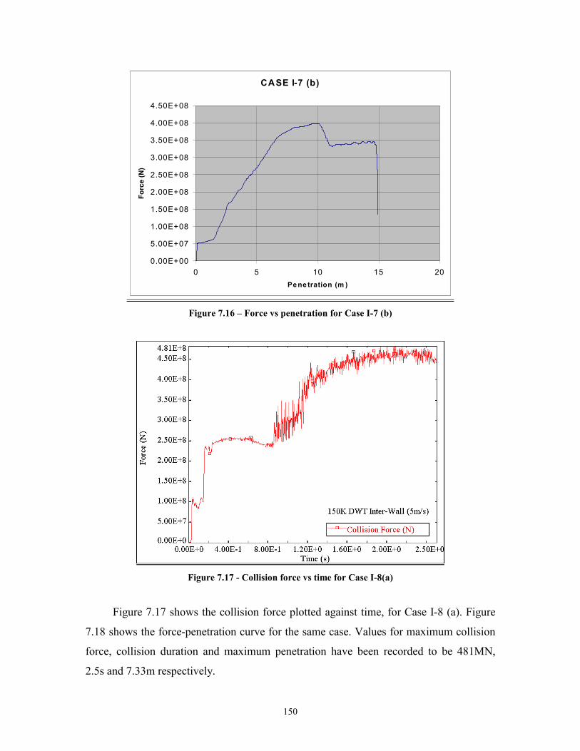
150
CASE I-7 (b)
0.00E+00
5.00E+07
1.00E+08
1.50E+08
2.00E+08
2.50E+08
3.00E+08
3.50E+08
4.00E+08
4.50E+08
0 5 10 15 20Penetration (m )
Forc
e (N
)
Figure 7.16 – Force vs penetration for Case I-7 (b)
Figure 7.17 - Collision force vs time for Case I-8(a)
Figure 7.17 shows the collision force plotted against time, for Case I-8 (a). Figure
7.18 shows the force-penetration curve for the same case. Values for maximum collision
force, collision duration and maximum penetration have been recorded to be 481MN,
2.5s and 7.33m respectively.
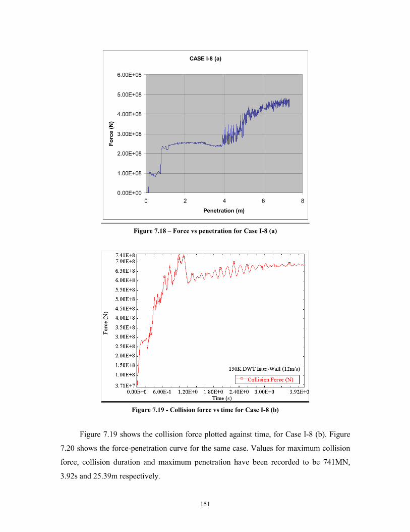
151
CASE I-8 (a)
0.00E+00
1.00E+08
2.00E+08
3.00E+08
4.00E+08
5.00E+08
6.00E+08
0 2 4 6 8
Penetration (m)
Forc
e (N
)
Figure 7.18 – Force vs penetration for Case I-8 (a)
Figure 7.19 - Collision force vs time for Case I-8 (b)
Figure 7.19 shows the collision force plotted against time, for Case I-8 (b). Figure
7.20 shows the force-penetration curve for the same case. Values for maximum collision
force, collision duration and maximum penetration have been recorded to be 741MN,
3.92s and 25.39m respectively.
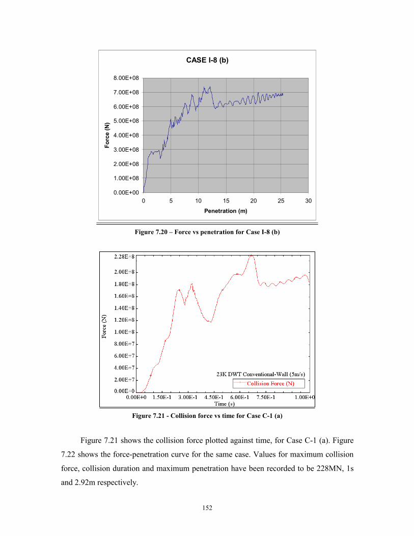
152
CASE I-8 (b)
0.00E+00
1.00E+08
2.00E+08
3.00E+08
4.00E+08
5.00E+08
6.00E+08
7.00E+08
8.00E+08
0 5 10 15 20 25 30
Penetration (m)
Forc
e (N
)
Figure 7.20 – Force vs penetration for Case I-8 (b)
Figure 7.21 - Collision force vs time for Case C-1 (a)
Figure 7.21 shows the collision force plotted against time, for Case C-1 (a). Figure
7.22 shows the force-penetration curve for the same case. Values for maximum collision
force, collision duration and maximum penetration have been recorded to be 228MN, 1s
and 2.92m respectively.
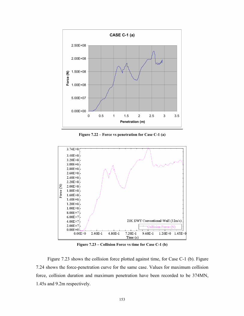
153
CASE C-1 (a)
0.00E+00
5.00E+07
1.00E+08
1.50E+08
2.00E+08
2.50E+08
0 0.5 1 1.5 2 2.5 3 3.5
Penetration (m)
Forc
e (N
)
Figure 7.22 – Force vs penetration for Case C-1 (a)
Figure 7.23 – Collision Force vs time for Case C-1 (b)
Figure 7.23 shows the collision force plotted against time, for Case C-1 (b). Figure
7.24 shows the force-penetration curve for the same case. Values for maximum collision
force, collision duration and maximum penetration have been recorded to be 374MN,
1.45s and 9.2m respectively.
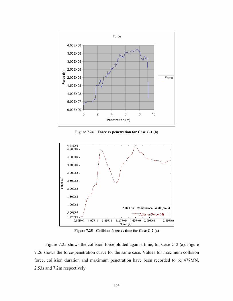
154
Force
0.00E+00
5.00E+07
1.00E+08
1.50E+08
2.00E+08
2.50E+08
3.00E+08
3.50E+08
4.00E+08
0 2 4 6 8 10
Penetration (m)
Forc
e (N
)
Force
Figure 7.24 – Force vs penetration for Case C-1 (b)
Figure 7.25 - Collision force vs time for Case C-2 (a)
Figure 7.25 shows the collision force plotted against time, for Case C-2 (a). Figure
7.26 shows the force-penetration curve for the same case. Values for maximum collision
force, collision duration and maximum penetration have been recorded to be 477MN,
2.53s and 7.2m respectively.
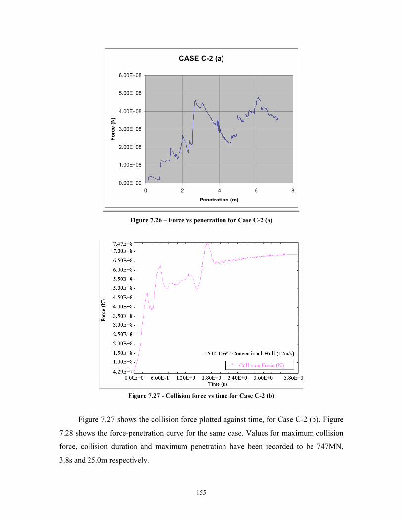
155
CASE C-2 (a)
0.00E+00
1.00E+08
2.00E+08
3.00E+08
4.00E+08
5.00E+08
6.00E+08
0 2 4 6 8
Penetration (m)
Forc
e (N
)
Figure 7.26 – Force vs penetration for Case C-2 (a)
Figure 7.27 - Collision force vs time for Case C-2 (b)
Figure 7.27 shows the collision force plotted against time, for Case C-2 (b). Figure
7.28 shows the force-penetration curve for the same case. Values for maximum collision
force, collision duration and maximum penetration have been recorded to be 747MN,
3.8s and 25.0m respectively.
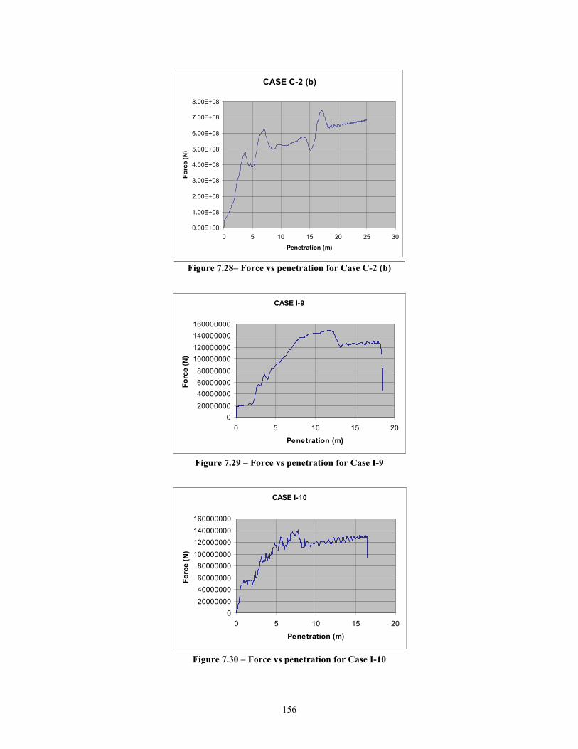
156
CASE C-2 (b)
0.00E+00
1.00E+08
2.00E+08
3.00E+08
4.00E+08
5.00E+08
6.00E+08
7.00E+08
8.00E+08
0 5 10 15 20 25 30Penetration (m)
Forc
e (N
)
Figure 7.28– Force vs penetration for Case C-2 (b)
CASE I-9
020000000400000006000000080000000
100000000120000000140000000160000000
0 5 10 15 20
Penetration (m)
Forc
e (N
)
Figure 7.29 – Force vs penetration for Case I-9
CASE I-10
020000000400000006000000080000000
100000000120000000140000000160000000
0 5 10 15 20
Penetration (m)
Forc
e (N
)
Figure 7.30 – Force vs penetration for Case I-10
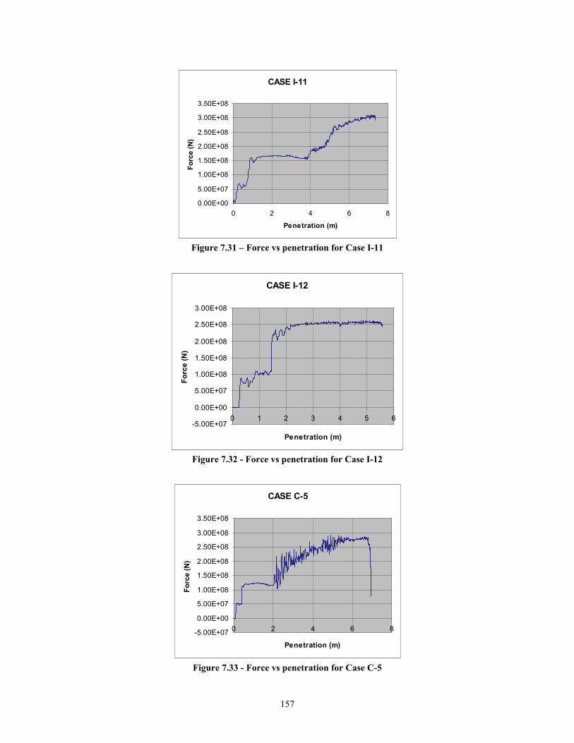
157
CASE I-11
0.00E+00
5.00E+07
1.00E+08
1.50E+08
2.00E+08
2.50E+08
3.00E+08
3.50E+08
0 2 4 6 8
Penetration (m)
Forc
e (N
)
Figure 7.31 – Force vs penetration for Case I-11
CASE I-12
-5.00E+07
0.00E+00
5.00E+07
1.00E+08
1.50E+08
2.00E+08
2.50E+08
3.00E+08
0 1 2 3 4 5 6
Penetration (m)
Forc
e (N
)
Figure 7.32 - Force vs penetration for Case I-12
CASE C-5
-5.00E+07
0.00E+00
5.00E+07
1.00E+08
1.50E+08
2.00E+08
2.50E+08
3.00E+08
3.50E+08
0 2 4 6 8
Penetration (m)
Forc
e (N
)
Figure 7.33 - Force vs penetration for Case C-5
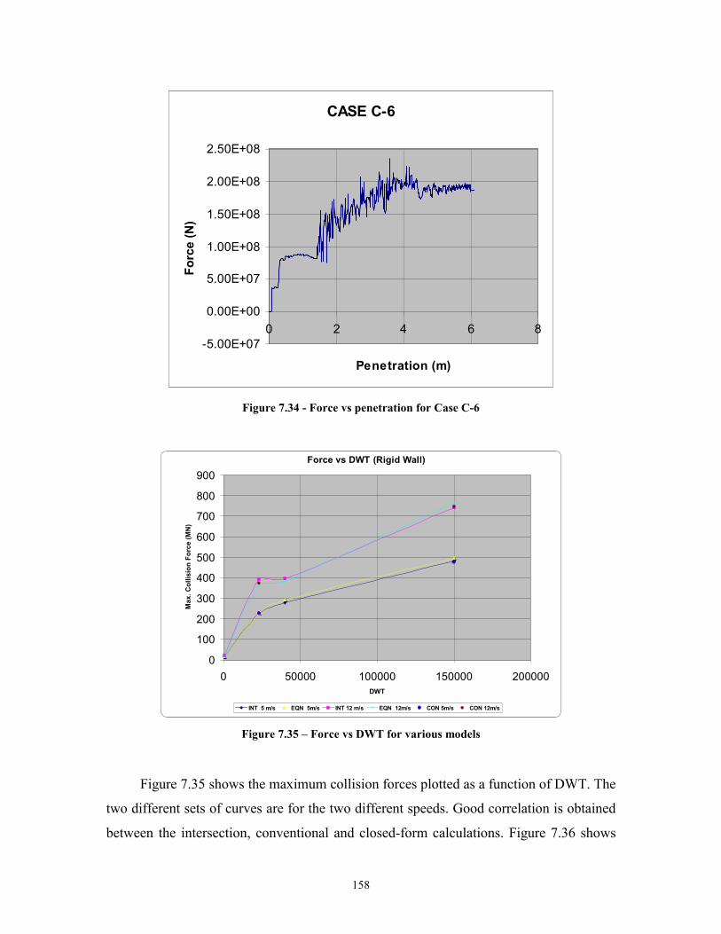
158
CASE C-6
-5.00E+07
0.00E+00
5.00E+07
1.00E+08
1.50E+08
2.00E+08
2.50E+08
0 2 4 6 8
Penetration (m)
Forc
e (N
)
Figure 7.34 - Force vs penetration for Case C-6
Force vs DWT (Rigid Wall)
0
100
200
300
400
500
600
700
800
900
0 50000 100000 150000 200000DWT
Max
. Col
lisio
n Fo
rce
(MN
)
INT 5 m/s EQN 5m/s INT 12 m/s EQN 12m/s CON 5m/s CON 12m/s
Figure 7.35 – Force vs DWT for various models
Figure 7.35 shows the maximum collision forces plotted as a function of DWT. The
two different sets of curves are for the two different speeds. Good correlation is obtained
between the intersection, conventional and closed-form calculations. Figure 7.36 shows
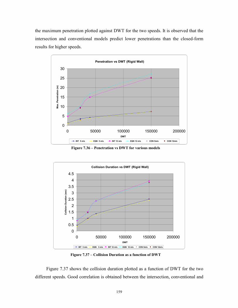
159
the maximum penetration plotted against DWT for the two speeds. It is observed that the
intersection and conventional models predict lower penetrations than the closed-form
results for higher speeds.
Penetration vs DWT (Rigid Wall)
0
5
10
15
20
25
30
0 50000 100000 150000 200000DWT
Max
. Pen
etra
tion
(m)
INT 5 m/s EQN 5 m/s INT 12 m/s EQN 12 m/s CON 5m/s CON 12m/s
Figure 7.36 – Penetration vs DWT for various models
Collision Duration vs DWT (Rigid Wall)
00.5
11.5
22.5
33.5
44.5
0 50000 100000 150000 200000DWT
Col
lisio
n D
urat
ion
(sec
)
INT 5 m/s EQN 5 m/s INT 12 m/s EQN 12 m/s CON 5m/s CON 12m/s Figure 7.37 – Collision Duration as a function of DWT
Figure 7.37 shows the collision duration plotted as a function of DWT for the two
different speeds. Good correlation is obtained between the intersection, conventional and
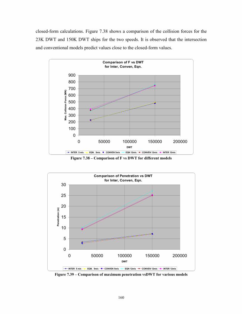
160
closed-form calculations. Figure 7.38 shows a comparison of the collision forces for the
23K DWT and 150K DWT ships for the two speeds. It is observed that the intersection
and conventional models predict values close to the closed-form values.
Comparison of F vs DWTfor Inter, Conven, Eqn.
0100200300400500600700800900
0 50000 100000 150000 200000DWT
Max
. Col
lisio
n Fo
rce
(MN
)
INTER 5 m/s EQN. 5m/s CONVEN 5m/s EQN 12m/s CONVEN 12m/s INTER 12m/s Figure 7.38 – Comparison of F vs DWT for different models
Comparison of Penetration vs DWTfor Inter, Conven, Eqn.
0
5
10
15
20
25
30
0 50000 100000 150000 200000DWT
Pene
trat
ion
(m)
INTER 5 m/s EQN. 5m/s CONVEN 5m/s EQN 12m/s CONVEN 12m/s INTER 12m/s Figure 7.39 – Comparison of maximum penetration vsDWT for various models
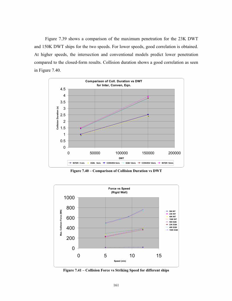
161
Figure 7.39 shows a comparison of the maximum penetration for the 23K DWT
and 150K DWT ships for the two speeds. For lower speeds, good correlation is obtained.
At higher speeds, the intersection and conventional models predict lower penetration
compared to the closed-form results. Collision duration shows a good correlation as seen
in Figure 7.40.
Comparison of Coll. Duration vs DWTfor Inter, Conven, Eqn.
0
0.5
11.5
2
2.5
33.5
44.5
0 50000 100000 150000 200000DWT
Col
lisio
n D
urat
ion
(s)
INTER 5 m/s EQN. 5m/s CONVEN 5m/s EQN 12m/s CONVEN 12m/s INTER 12m/s
Figure 7.40 – Comparison of Collision Duration vs DWT
Force vs Speed (Rigid Wall)
0
200
400
600
800
1000
0 5 10 15Speed (m/s)
Max
. Col
lisio
n Fo
rce
(MN
)
500 INT23K INT40K INT150K INT500 EQN23K EQN40K EQN150K EQN
Figure 7.41 – Collision Force vs Striking Speed for different ships
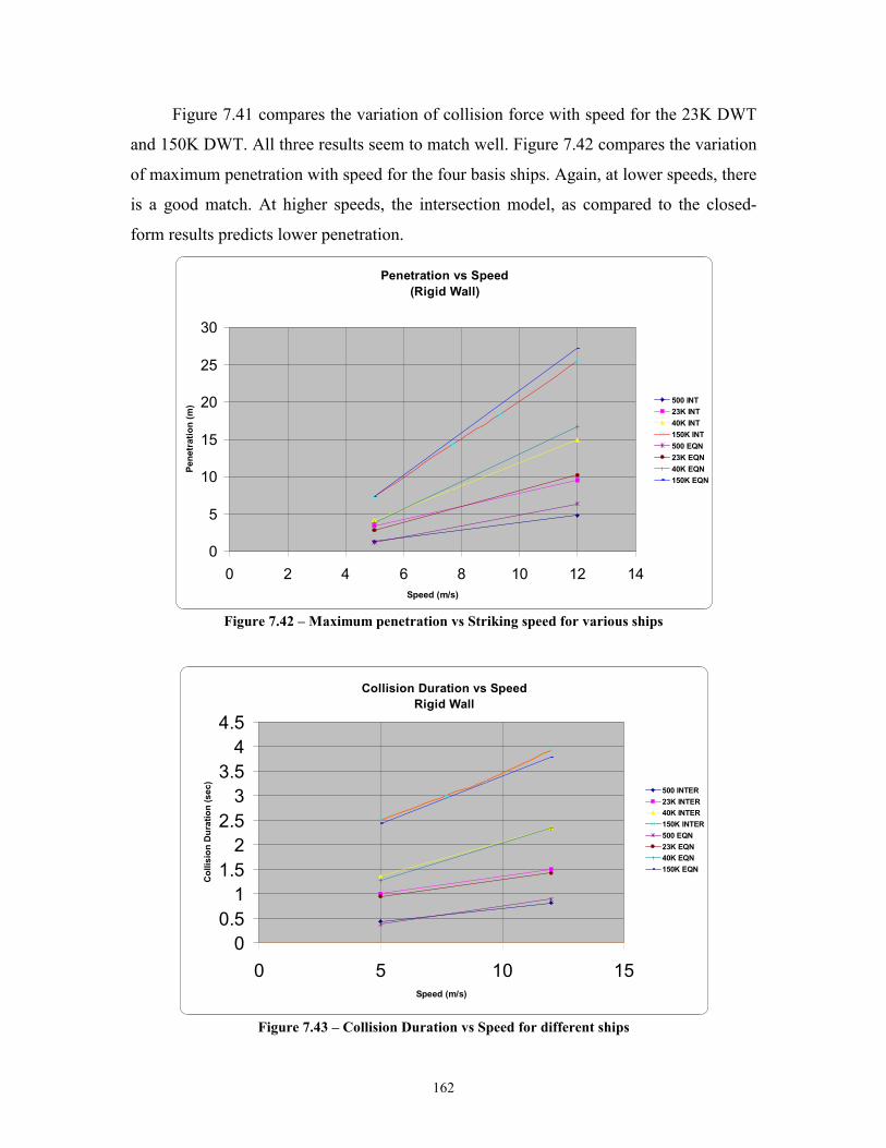
162
Figure 7.41 compares the variation of collision force with speed for the 23K DWT
and 150K DWT. All three results seem to match well. Figure 7.42 compares the variation
of maximum penetration with speed for the four basis ships. Again, at lower speeds, there
is a good match. At higher speeds, the intersection model, as compared to the closed-
form results predicts lower penetration.
Penetration vs Speed(Rigid Wall)
0
5
10
15
20
25
30
0 2 4 6 8 10 12 14Speed (m/s)
Pene
trat
ion
(m) 500 INT
23K INT40K INT150K INT500 EQN23K EQN40K EQN150K EQN
Figure 7.42 – Maximum penetration vs Striking speed for various ships
Collision Duration vs SpeedRigid Wall
00.5
11.5
22.5
33.5
44.5
0 5 10 15Speed (m/s)
Col
lisio
n D
urat
ion
(sec
)
500 INTER23K INTER40K INTER150K INTER500 EQN23K EQN40K EQN150K EQN
Figure 7.43 – Collision Duration vs Speed for different ships
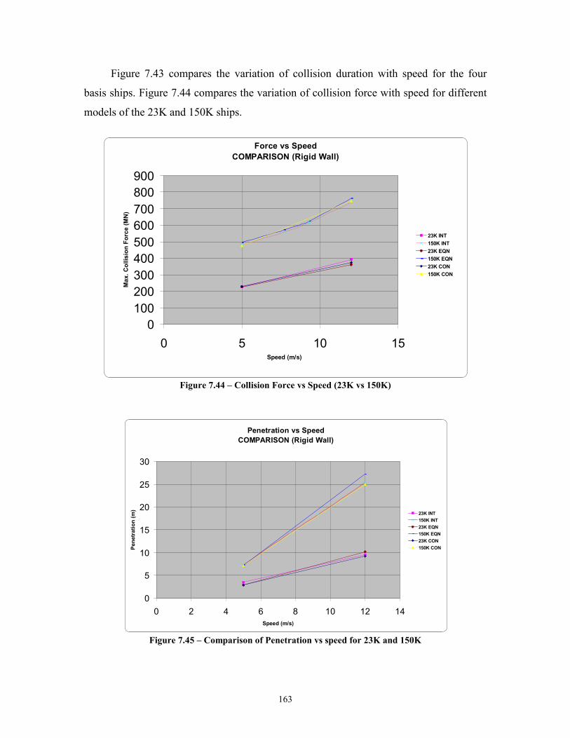
163
Figure 7.43 compares the variation of collision duration with speed for the four
basis ships. Figure 7.44 compares the variation of collision force with speed for different
models of the 23K and 150K ships.
Force vs SpeedCOMPARISON (Rigid Wall)
0100200300400500600700800900
0 5 10 15Speed (m/s)
Max
. Col
lisio
n Fo
rce
(MN
)
23K INT150K INT23K EQN150K EQN23K CON150K CON
Figure 7.44 – Collision Force vs Speed (23K vs 150K)
Penetration vs SpeedCOMPARISON (Rigid Wall)
0
5
10
15
20
25
30
0 2 4 6 8 10 12 14Speed (m/s)
Pene
tratio
n (m
)
23K INT150K INT23K EQN150K EQN23K CON150K CON
Figure 7.45 – Comparison of Penetration vs speed for 23K and 150K
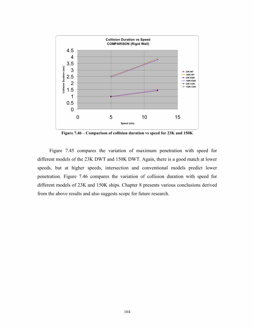
164
Collision Duration vs SpeedCOMPARISON (Rigid Wall)
00.5
11.5
22.5
33.5
44.5
0 5 10 15Speed (m/s)
Col
lisio
n D
urat
ion
(sec
)
23K INT150K INT23K EQN150K EQN23K CON150K CON
Figure 7.46 – Comparison of collision duration vs speed for 23K and 150K
Figure 7.45 compares the variation of maximum penetration with speed for
different models of the 23K DWT and 150K DWT. Again, there is a good match at lower
speeds, but at higher speeds, intersection and conventional models predict lower
penetration. Figure 7.46 compares the variation of collision duration with speed for
different models of 23K and 150K ships. Chapter 8 presents various conclusions derived
from the above results and also suggests scope for future research.
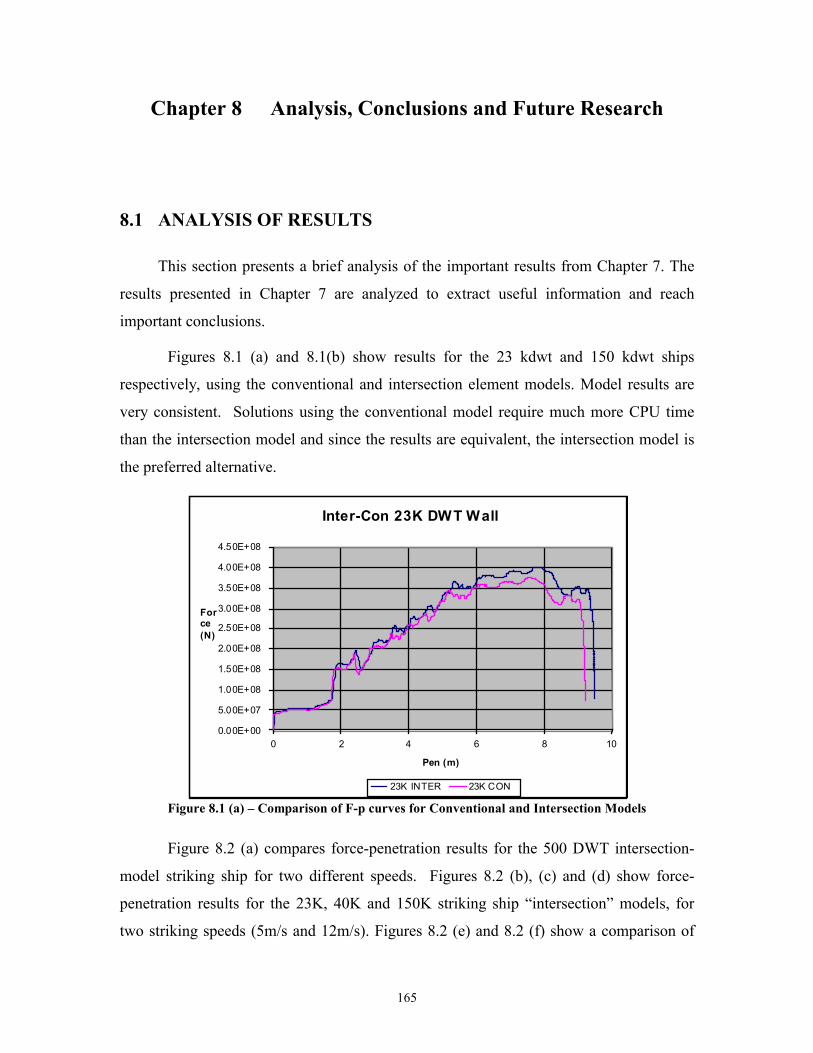
165
Chapter 8 Analysis, Conclusions and Future Research 8.1 ANALYSIS OF RESULTS
This section presents a brief analysis of the important results from Chapter 7. The
results presented in Chapter 7 are analyzed to extract useful information and reach
important conclusions.
Figures 8.1 (a) and 8.1(b) show results for the 23 kdwt and 150 kdwt ships
respectively, using the conventional and intersection element models. Model results are
very consistent. Solutions using the conventional model require much more CPU time
than the intersection model and since the results are equivalent, the intersection model is
the preferred alternative.
Inter-Con 23K DWT Wall
0.00E+00
5.00E+07
1.00E+08
1.50E+08
2.00E+08
2.50E+08
3.00E+08
3.50E+08
4.00E+08
4.50E+08
0 2 4 6 8 10
Pen (m)
Force(N)
23K INTER 23K CON
Figure 8.1 (a) – Comparison of F-p curves for Conventional and Intersection Models
Figure 8.2 (a) compares force-penetration results for the 500 DWT intersection-
model striking ship for two different speeds. Figures 8.2 (b), (c) and (d) show force-
penetration results for the 23K, 40K and 150K striking ship “intersection” models, for
two striking speeds (5m/s and 12m/s). Figures 8.2 (e) and 8.2 (f) show a comparison of
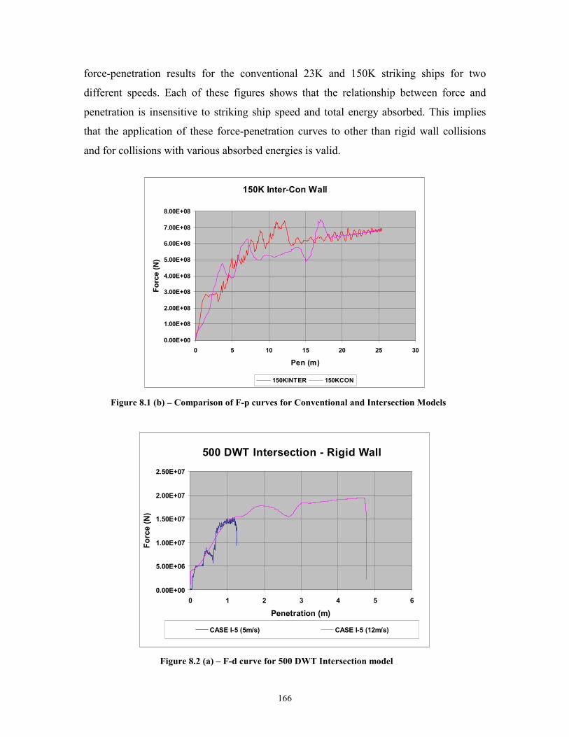
166
force-penetration results for the conventional 23K and 150K striking ships for two
different speeds. Each of these figures shows that the relationship between force and
penetration is insensitive to striking ship speed and total energy absorbed. This implies
that the application of these force-penetration curves to other than rigid wall collisions
and for collisions with various absorbed energies is valid.
150K Inter-Con Wall
0.00E+00
1.00E+08
2.00E+08
3.00E+08
4.00E+08
5.00E+08
6.00E+08
7.00E+08
8.00E+08
0 5 10 15 20 25 30
Pen (m)
Forc
e (N
)
150KINTER 150KCON
Figure 8.1 (b) – Comparison of F-p curves for Conventional and Intersection Models
500 DWT Intersection - Rigid Wall
0.00E+00
5.00E+06
1.00E+07
1.50E+07
2.00E+07
2.50E+07
0 1 2 3 4 5 6
Penetration (m)
Forc
e (N
)
CASE I-5 (5m/s) CASE I-5 (12m/s)
Figure 8.2 (a) – F-d curve for 500 DWT Intersection model
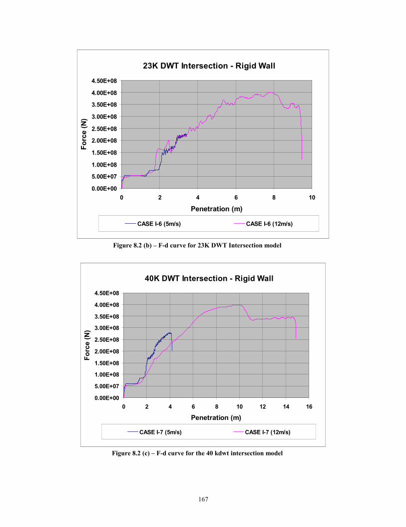
167
23K DWT Intersection - Rigid Wall
0.00E+00
5.00E+07
1.00E+08
1.50E+08
2.00E+08
2.50E+08
3.00E+08
3.50E+08
4.00E+08
4.50E+08
0 2 4 6 8 10
Penetration (m)
Forc
e (N
)
CASE I-6 (5m/s) CASE I-6 (12m/s)
Figure 8.2 (b) – F-d curve for 23K DWT Intersection model
40K DWT Intersection - Rigid Wall
0.00E+00
5.00E+07
1.00E+08
1.50E+08
2.00E+08
2.50E+08
3.00E+08
3.50E+08
4.00E+08
4.50E+08
0 2 4 6 8 10 12 14 16
Penetration (m)
Forc
e (N
)
CASE I-7 (5m/s) CASE I-7 (12m/s)
Figure 8.2 (c) – F-d curve for the 40 kdwt intersection model
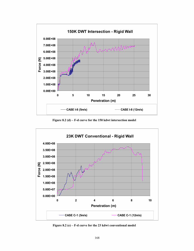
168
150K DWT Intersection - Rigid Wall
0.00E+00
1.00E+08
2.00E+08
3.00E+08
4.00E+08
5.00E+08
6.00E+08
7.00E+08
8.00E+08
0 5 10 15 20 25 30
Penetration (m)
Forc
e (N
)
CASE I-8 (5m/s) CASE I-8 (12m/s)
Figure 8.2 (d) – F-d curve for the 150 kdwt intersection model
23K DWT Conventional - Rigid Wall
0.00E+00
5.00E+07
1.00E+08
1.50E+08
2.00E+08
2.50E+08
3.00E+08
3.50E+08
4.00E+08
0 2 4 6 8 10
Penetration (m)
Forc
e (N
)
CASE C-1 (5m/s) CASE C-1 (12m/s)
Figure 8.2 (e) – F-d curve for the 23 kdwt conventional model
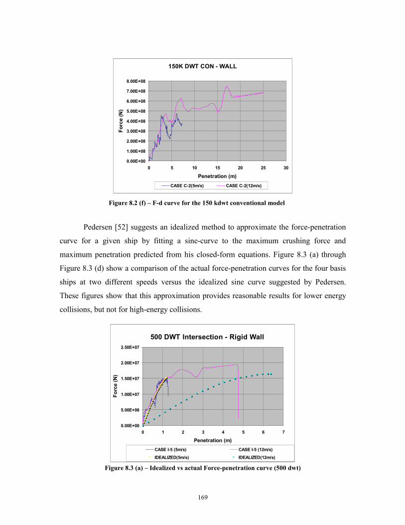
169
150K DWT CON - WALL
0.00E+00
1.00E+08
2.00E+08
3.00E+08
4.00E+08
5.00E+08
6.00E+08
7.00E+08
8.00E+08
0 5 10 15 20 25 30
Penetration (m)
Forc
e (N
)
CASE C-2(5m/s) CASE C-2(12m/s)
Figure 8.2 (f) – F-d curve for the 150 kdwt conventional model
Pedersen [52] suggests an idealized method to approximate the force-penetration
curve for a given ship by fitting a sine-curve to the maximum crushing force and
maximum penetration predicted from his closed-form equations. Figure 8.3 (a) through
Figure 8.3 (d) show a comparison of the actual force-penetration curves for the four basis
ships at two different speeds versus the idealized sine curve suggested by Pedersen.
These figures show that this approximation provides reasonable results for lower energy
collisions, but not for high-energy collisions.
500 DWT Intersection - Rigid Wall
0.00E+00
5.00E+06
1.00E+07
1.50E+07
2.00E+07
2.50E+07
0 1 2 3 4 5 6 7
Penetration (m)
Forc
e (N
)
CASE I-5 (5m/s) CASE I-5 (12m/s)
IDEALIZED(5m/s) IDEALIZED(12m/s) Figure 8.3 (a) – Idealized vs actual Force-penetration curve (500 dwt)
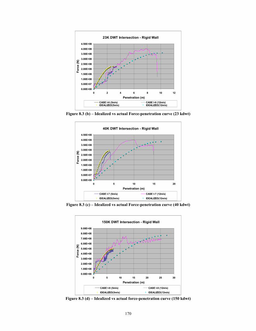
170
23K DWT Intersection - Rigid Wall
0.00E+00
5.00E+07
1.00E+08
1.50E+08
2.00E+08
2.50E+08
3.00E+08
3.50E+08
4.00E+08
4.50E+08
0 2 4 6 8 10 12
Penetration (m)
Forc
e (N
)
CASE I-6 (5m/s) CASE I-6 (12m/s)IDEALIZED(5m/s) IDEALIZED(12m/s)
Figure 8.3 (b) – Idealized vs actual Force-penetration curve (23 kdwt)
40K DWT Intersection - Rigid Wall
0.00E+00
5.00E+07
1.00E+08
1.50E+08
2.00E+08
2.50E+08
3.00E+08
3.50E+08
4.00E+08
4.50E+08
0 5 10 15 20
Penetration (m)
Forc
e (N
)
CASE I-7 (5m/s) CASE I-7 (12m/s)IDEALIZED(5m/s) IDEALIZED(12m/s)
Figure 8.3 (c) – Idealized vs actual Force-penetration curve (40 kdwt)
150K DWT Intersection - Rigid Wall
0.00E+00
1.00E+08
2.00E+08
3.00E+08
4.00E+08
5.00E+08
6.00E+08
7.00E+08
8.00E+08
9.00E+08
0 5 10 15 20 25 30
Penetration (m)
Forc
e (N
)
CASE I-8 (5m/s) CASE I-8 (12m/s)IDEALIZED(5m/s) IDEALIZED(12m/s)
Figure 8.3 (d) – Idealized vs actual force-penetration curve (150 kdwt)
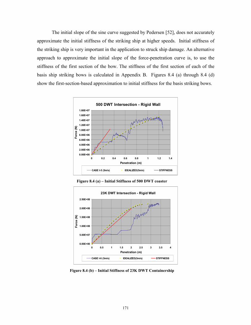
171
The initial slope of the sine curve suggested by Pedersen [52], does not accurately
approximate the initial stiffness of the striking ship at higher speeds. Initial stiffness of
the striking ship is very important in the application to struck ship damage. An alternative
approach to approximate the initial slope of the force-penetration curve is, to use the
stiffness of the first section of the bow. The stiffness of the first section of each of the
basis ship striking bows is calculated in Appendix B. Figures 8.4 (a) through 8.4 (d)
show the first-section-based approximation to initial stiffness for the basis striking bows.
500 DWT Intersection - Rigid Wall
0.00E+00
2.00E+06
4.00E+06
6.00E+06
8.00E+06
1.00E+07
1.20E+07
1.40E+07
1.60E+07
1.80E+07
0 0.2 0.4 0.6 0.8 1 1.2 1.4
Penetration (m)
Forc
e (N
)
CASE I-5 (5m/s) IDEALIZED(5m/s) STIFFNESS
Figure 8.4 (a) – Initial Stiffness of 500 DWT coaster
23K DWT Intersection - Rigid Wall
0.00E+00
5.00E+07
1.00E+08
1.50E+08
2.00E+08
2.50E+08
0 0.5 1 1.5 2 2.5 3 3.5 4
Penetration (m)
Forc
e (N
)
CASE I-6 (5m/s) IDEALIZED(5m/s) STIFFNESS
Figure 8.4 (b) – Initial Stiffness of 23K DWT Containership
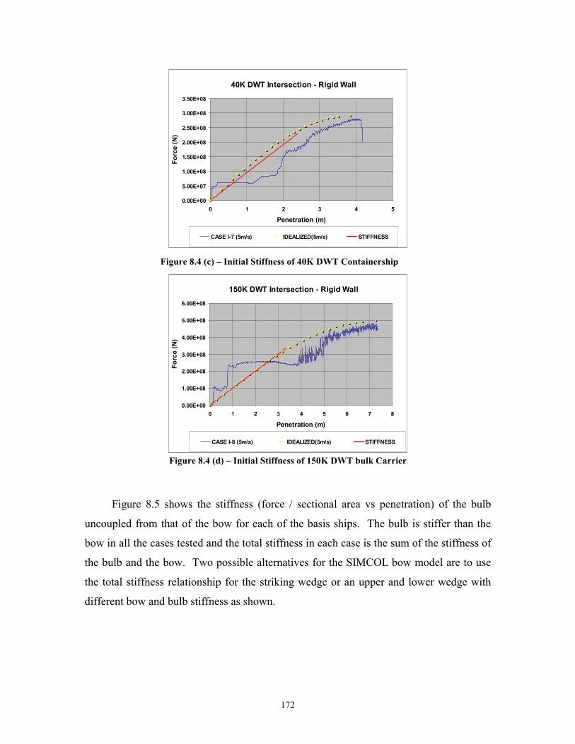
172
40K DWT Intersection - Rigid Wall
0.00E+00
5.00E+07
1.00E+08
1.50E+08
2.00E+08
2.50E+08
3.00E+08
3.50E+08
0 1 2 3 4 5
Penetration (m)
Forc
e (N
)
CASE I-7 (5m/s) IDEALIZED(5m/s) STIFFNESS
Figure 8.4 (c) – Initial Stiffness of 40K DWT Containership
150K DWT Intersection - Rigid Wall
0.00E+00
1.00E+08
2.00E+08
3.00E+08
4.00E+08
5.00E+08
6.00E+08
0 1 2 3 4 5 6 7 8
Penetration (m)
Forc
e (N
)
CASE I-8 (5m/s) IDEALIZED(5m/s) STIFFNESS
Figure 8.4 (d) – Initial Stiffness of 150K DWT bulk Carrier
Figure 8.5 shows the stiffness (force / sectional area vs penetration) of the bulb
uncoupled from that of the bow for each of the basis ships. The bulb is stiffer than the
bow in all the cases tested and the total stiffness in each case is the sum of the stiffness of
the bulb and the bow. Two possible alternatives for the SIMCOL bow model are to use
the total stiffness relationship for the striking wedge or an upper and lower wedge with
different bow and bulb stiffness as shown.
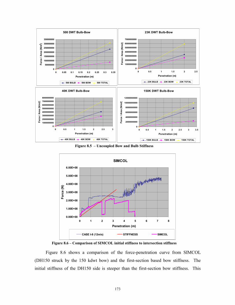
173
500 DWT Bulb-Bow
0
50000000
100000000
150000000
200000000
250000000
300000000
350000000
0 0.05 0.1 0.15 0.2 0.25 0.3 0.35
Penetration (m)
Forc
e / A
rea
(N/m
2 )
500 BULB 500 BOW 500 TOTAL
23K DWT Bulb-Bow
0
1000000000
2000000000
3000000000
4000000000
5000000000
6000000000
7000000000
0 0.5 1 1.5 2 2.5
Penetration (m)
Forc
e / A
rea
(N/m
2)
23K BULB 23K BOW 23K TOTAL
40K DWT Bulb-Bow
010000000002000000000300000000040000000005000000000600000000070000000008000000000
0 0.5 1 1.5 2 2.5 3
Penetration (m)
Forc
e / A
rea
(N/m
2)
40K BULB 40K BOW 40K TOTAL
150K DWT Bulb-Bow
0
2000000000
4000000000
6000000000
8000000000
10000000000
12000000000
0 0.5 1 1.5 2 2.5 3 3.5
Penetration (m)
Forc
e / A
rea
(N/m
2)
150K BULB 150K BOW 150K TOTAL
Figure 8.5 – Uncoupled Bow and Bulb Stiffness
SIMCOL
0.00E+00
1.00E+08
2.00E+08
3.00E+08
4.00E+08
5.00E+08
6.00E+08
0 1 2 3 4 5 6 7 8
Penetration (m)
Forc
e (N
)
CASE I-8 (12m/s) STIFFNESS SIMCOL
Figure 8.6 – Comparison of SIMCOL initial stiffness to intersection stiffness
Figure 8.6 shows a comparison of the force-penetration curve from SIMCOL
(DH150 struck by the 150 kdwt bow) and the first-section based bow stiffness. The
initial stiffness of the DH150 side is steeper than the first-section bow stiffness. This
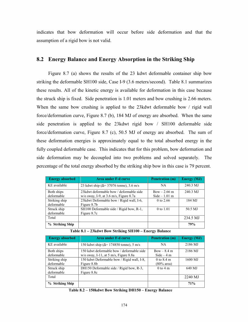
174
indicates that bow deformation will occur before side deformation and that the
assumption of a rigid bow is not valid.
8.2 Energy Balance and Energy Absorption in the Striking Ship
Figure 8.7 (a) shows the results of the 23 kdwt deformable container ship bow
striking the deformable SH100 side, Case I-9 (3.6 meters/second). Table 8.1 summarizes
these results. All of the kinetic energy is available for deformation in this case because
the struck ship is fixed. Side penetration is 1.01 meters and bow crushing is 2.66 meters.
When the same bow crushing is applied to the 23kdwt deformable bow / rigid wall
force/deformation curve, Figure 8.7 (b), 184 MJ of energy are absorbed. When the same
side penetration is applied to the 23kdwt rigid bow / SH100 deformable side
force/deformation curve, Figure 8.7 (c), 50.5 MJ of energy are absorbed. The sum of
these deformation energies is approximately equal to the total absorbed energy in the
fully coupled deformable case. This indicates that for this problem, bow deformation and
side deformation may be decoupled into two problems and solved separately. The
percentage of the total energy absorbed by the striking ship bow in this case is 79 percent.
Energy absorbed Area under F-d curve Penetration (m) Energy (MJ)
KE available 23 kdwt ship (∆= 37076 tonne), 3.6 m/s NA 240.3 MJ
Both ships deformable
23kdwt deformable bow / deformable side w/o sway, I-9, at 3.6 m/s, Figure 8.7a
Bow – 2.66 m Side – 1.01 m
240.3 MJ
Striking ship deformable
23kdwt Deformable bow / Rigid wall, I-6, Figure 8.7b
0 to 2.66 184 MJ
Struck ship deformable
SH100 Deformable side / Rigid bow, R-1, Figure 8.7c
0 to 1.01 50.5 MJ
Total 234.5 MJ % Striking Ship 79%
Table 8.1 – 23kdwt Bow Striking SH100 – Energy Balance
Energy absorbed Area under F-d curve Penetration (m) Energy (MJ)
KE available 150 kdwt ship (∆= 174850 tonne), 5 m/s NA 2186 MJ
Both ships deformable
150 kdwt deformable bow / deformable side w/o sway, I-11, at 5 m/s, Figure 8.8a
Bow – 8.4 m Side – 4 m
2186 MJ
Striking ship deformable
150 kdwt Deformable bow / Rigid wall, I-8, Figure 8.8b
0 to 8.4 m (80% area)
1600 MJ
Struck ship deformable
DH150 Deformable side / Rigid bow, R-3, Figure 8.8c
0 to 4 m 640 MJ
Total 2240 MJ % Striking Ship 71%
Table 8.2 – 150kdwt Bow Striking DH150 – Energy Balance
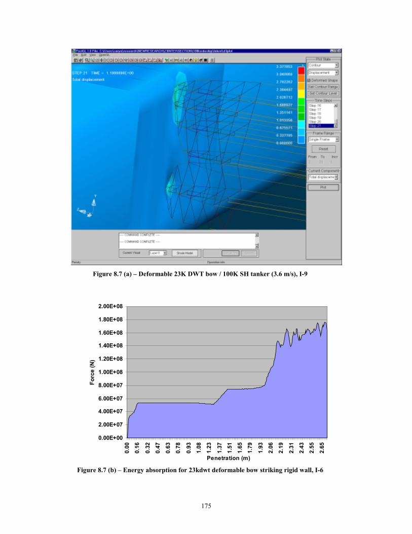
175
Figure 8.7 (a) – Deformable 23K DWT bow / 100K SH tanker (3.6 m/s), I-9
0.00E+00
2.00E+07
4.00E+07
6.00E+07
8.00E+07
1.00E+08
1.20E+08
1.40E+08
1.60E+08
1.80E+08
2.00E+08
0.00
0.16
0.32
0.47
0.63
0.78
0.93
1.08
1.23
1.37
1.51
1.65
1.79
1.93
2.06
2.19
2.31
2.43
2.55
2.65
Penetration (m)
Forc
e (N
)
Figure 8.7 (b) – Energy absorption for 23kdwt deformable bow striking rigid wall, I-6
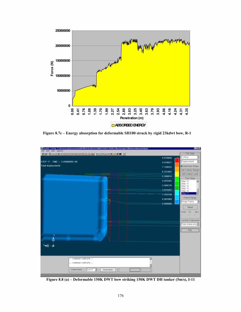
176
0
50000000
100000000
150000000
200000000
250000000
0.00
0.41
0.76
1.08
1.39
1.70
1.99
2.27
2.54
2.80
3.03
3.25
3.45
3.63
3.79
3.93
4.06
4.16
4.24
4.31
4.35
Penetration (m)
Forc
e (N
)
ABSORBED ENERGY Figure 8.7c – Energy absorption for deformable SH100 struck by rigid 23kdwt bow, R-1
Figure 8.8 (a) – Deformable 150K DWT bow striking 150K DWT DH tanker (5m/s), I-11
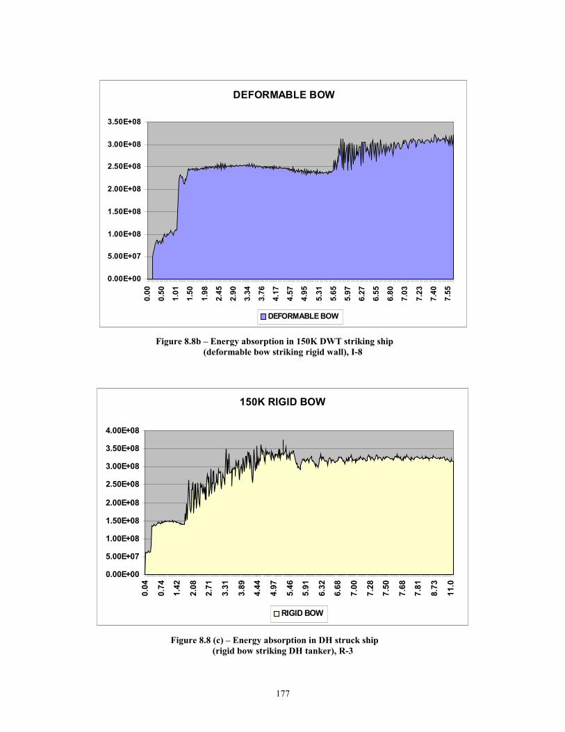
177
DEFORMABLE BOW
0.00E+00
5.00E+07
1.00E+08
1.50E+08
2.00E+08
2.50E+08
3.00E+08
3.50E+08
0.00
0.50
1.01
1.50
1.98
2.45
2.90
3.34
3.76
4.17
4.57
4.95
5.31
5.65
5.97
6.27
6.55
6.80
7.03
7.23
7.40
7.55
DEFORMABLE BOW
Figure 8.8b – Energy absorption in 150K DWT striking ship (deformable bow striking rigid wall), I-8
150K RIGID BOW
0.00E+00
5.00E+07
1.00E+08
1.50E+08
2.00E+08
2.50E+08
3.00E+08
3.50E+08
4.00E+08
0.04
0.74
1.42
2.08
2.71
3.31
3.89
4.44
4.97
5.46
5.91
6.32
6.68
7.00
7.28
7.50
7.68
7.81
8.73
11.0
RIGID BOW
Figure 8.8 (c) – Energy absorption in DH struck ship (rigid bow striking DH tanker), R-3
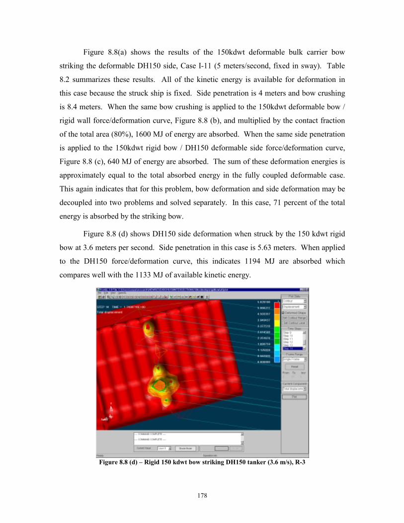
178
Figure 8.8(a) shows the results of the 150kdwt deformable bulk carrier bow
striking the deformable DH150 side, Case I-11 (5 meters/second, fixed in sway). Table
8.2 summarizes these results. All of the kinetic energy is available for deformation in
this case because the struck ship is fixed. Side penetration is 4 meters and bow crushing
is 8.4 meters. When the same bow crushing is applied to the 150kdwt deformable bow /
rigid wall force/deformation curve, Figure 8.8 (b), and multiplied by the contact fraction
of the total area (80%), 1600 MJ of energy are absorbed. When the same side penetration
is applied to the 150kdwt rigid bow / DH150 deformable side force/deformation curve,
Figure 8.8 (c), 640 MJ of energy are absorbed. The sum of these deformation energies is
approximately equal to the total absorbed energy in the fully coupled deformable case.
This again indicates that for this problem, bow deformation and side deformation may be
decoupled into two problems and solved separately. In this case, 71 percent of the total
energy is absorbed by the striking bow.
Figure 8.8 (d) shows DH150 side deformation when struck by the 150 kdwt rigid
bow at 3.6 meters per second. Side penetration in this case is 5.63 meters. When applied
to the DH150 force/deformation curve, this indicates 1194 MJ are absorbed which
compares well with the 1133 MJ of available kinetic energy.
Figure 8.8 (d) – Rigid 150 kdwt bow striking DH150 tanker (3.6 m/s), R-3
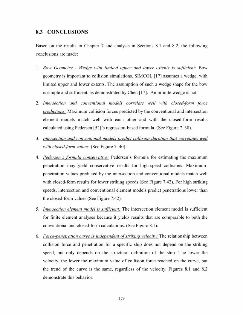
179
8.3 CONCLUSIONS
Based on the results in Chapter 7 and analysis in Sections 8.1 and 8.2, the following
conclusions are made:
1. Bow Geometry - Wedge with limited upper and lower extents is sufficient: Bow
geometry is important to collision simulations. SIMCOL [17] assumes a wedge, with
limited upper and lower extents. The assumption of such a wedge shape for the bow
is simple and sufficient, as demonstrated by Chen [17]. An infinite wedge is not.
2. Intersection and conventional models correlate well with closed-form force
predictions: Maximum collision forces predicted by the conventional and intersection
element models match well with each other and with the closed-form results
calculated using Pedersen [52]’s regression-based formula. (See Figure 7. 38).
3. Intersection and conventional models predict collision duration that correlates well
with closed-form values. (See Figure 7. 40).
4. Pedersen’s formula conservative: Pedersen’s formula for estimating the maximum
penetration may yield conservative results for high-speed collisions. Maximum-
penetration values predicted by the intersection and conventional models match well
with closed-form results for lower striking speeds (See Figure 7.42). For high striking
speeds, intersection and conventional element models predict penetrations lower than
the closed-form values (See Figure 7.42).
5. Intersection element model is sufficient: The intersection element model is sufficient
for finite element analyses because it yields results that are comparable to both the
conventional and closed-form calculations. (See Figure 8.1).
6. Force-penetration curve is independent of striking velocity: The relationship between
collision force and penetration for a specific ship does not depend on the striking
speed, but only depends on the structural definition of the ship. The lower the
velocity, the lower the maximum value of collision force reached on the curve, but
the trend of the curve is the same, regardless of the velocity. Figures 8.1 and 8.2
demonstrate this behavior.
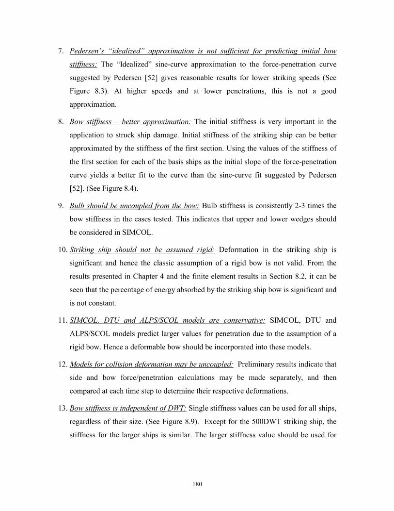
180
7. Pedersen’s “idealized” approximation is not sufficient for predicting initial bow
stiffness: The “Idealized” sine-curve approximation to the force-penetration curve
suggested by Pedersen [52] gives reasonable results for lower striking speeds (See
Figure 8.3). At higher speeds and at lower penetrations, this is not a good
approximation.
8. Bow stiffness – better approximation: The initial stiffness is very important in the
application to struck ship damage. Initial stiffness of the striking ship can be better
approximated by the stiffness of the first section. Using the values of the stiffness of
the first section for each of the basis ships as the initial slope of the force-penetration
curve yields a better fit to the curve than the sine-curve fit suggested by Pedersen
[52]. (See Figure 8.4).
9. Bulb should be uncoupled from the bow: Bulb stiffness is consistently 2-3 times the
bow stiffness in the cases tested. This indicates that upper and lower wedges should
be considered in SIMCOL.
10. Striking ship should not be assumed rigid: Deformation in the striking ship is
significant and hence the classic assumption of a rigid bow is not valid. From the
results presented in Chapter 4 and the finite element results in Section 8.2, it can be
seen that the percentage of energy absorbed by the striking ship bow is significant and
is not constant.
11. SIMCOL, DTU and ALPS/SCOL models are conservative: SIMCOL, DTU and
ALPS/SCOL models predict larger values for penetration due to the assumption of a
rigid bow. Hence a deformable bow should be incorporated into these models.
12. Models for collision deformation may be uncoupled: Preliminary results indicate that
side and bow force/penetration calculations may be made separately, and then
compared at each time step to determine their respective deformations.
13. Bow stiffness is independent of DWT: Single stiffness values can be used for all ships,
regardless of their size. (See Figure 8.9). Except for the 500DWT striking ship, the
stiffness for the larger ships is similar. The larger stiffness value should be used for
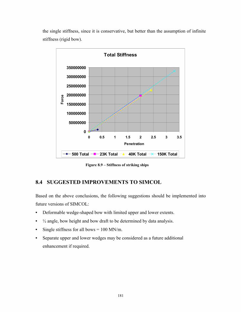
181
the single stiffness, since it is conservative, but better than the assumption of infinite
stiffness (rigid bow).
Total Stiffness
0
50000000
100000000
150000000
200000000
250000000
300000000
350000000
0 0.5 1 1.5 2 2.5 3 3.5
Penetration
Forc
e
500 Total 23K Total 40K Total 150K Total
Figure 8.9 – Stiffness of striking ships
8.4 SUGGESTED IMPROVEMENTS TO SIMCOL
Based on the above conclusions, the following suggestions should be implemented into
future versions of SIMCOL:
• = Deformable wedge-shaped bow with limited upper and lower extents.
• = ½ angle, bow height and bow draft to be determined by data analysis.
• = Single stiffness for all bows = 100 MN/m.
• = Separate upper and lower wedges may be considered as a future additional
enhancement if required.
182
8.5 FUTURE RESEARCH
1. The half-angle measurement is critical to collision calculations. A more rigorous
method should be proposed to define the half-angle for striking bows based on
penetrating volume.
2. Develop a simplified struck-ship side model for simulation with LS-DYNA. The
simplified models developed for the struck-ship side did not give consistent results.
Future research should consider using a super-element approach consistent with the
elements available in LS-DYNA.
3. Define a regression-based formula to predict the ship scenario parameters, given the
type of ship and DWT as described in Chapter 2.
4. Consider oblique angle collisions in LS-DYNA models.
5. Investigate transversely-stiffened bows.
183
REFERENCES
[1] J. Sirkar et al., “A Framework for Assessing the Environmental Performance of
Tankers in Accidental Groundings and Collisions”, presented at the SNAME
Annual Meeting, October 1997
[2] C. Rawson, K. Crake and A.J. Brown, “Assessing the Environmental Performance
of Tankers in Accidental Grounding and Collision” presented at the SNAME
Annual Meeting, November 1998
[3] A.J. Brown and M. Amrozowicz, “Tanker Environmental Risk - Putting the
Pieces Together”, SNAME/SNAJ International Conference on Designs and
Methodologies for Collision and Grounding Protection of Ships, August 1996
[4] IMO, “Interim Guidelines for Approval of Alternative Methods of Design and
Construction of Oil Tankers under Regulation 13F(5) of Annex I of MARPOL
73/78”, Resolution MEPC.66 (37), Adopted September 14, 1995
[5] Amdahl, J. (1983), "Energy Absorption in Ship Platform Impacts", Dr. Ing.
Thesis, Report No. UR-83-84, Norwegian Institute of Technology
[6] Amdahl, J. and Kavlie, D. (1992), “Experimental and Numerical Simulation of
Double Hull Stranding”, Proceedings of the DNV-MIT Workshop on “Mechanics
of Ship Collision and Grounding”, Oslo
[7] Amdahl, J. and Kavlie, D. (1995), “Design of Tankers for Grounding and
Collision”, MARIENV ’95, 1995.
[8] Ammerman, D.J. and Daidola, J.C (1996), “A Comparison of Methods for
Evaluating Structure During Ship Collisions”, Proceedings of the Intl. Conference
on Design and Methodologies for Collision and Grounding Protection of Ships,
San Francisco, August 1996
184
[9] Ammerman, D.J., Koski, J.A., Sprung, J.L.,, (1997), “SeaRAM: A US DOE
Study of Maritime Risk Assessment Data and Methods of Analysis”, Sandia
National Laboratories
[10] Arita, K (1994), “A Probabilistic Assessment on Protective Structures in Ship
Collisions”, 63 General Meeting of Ship Research Institute
[11] Arita, K. and Shoji Kuniaki (1995), “Expected Effectiveness of Double Side
Structures in Ship Collisions”, MARIENV’95, 1995
[12] Bach-Gansmo, O. and Valsgard S., “Simplified stiffness evaluation of a bulbous
ship bow”, Progress report No. 1, DnV, Report No. 81-0437 (1981). (Rev. no. 1
of 17.02.82)
[13] Bockenhauer, M. and Egge, E.D. (1995), “Assessment of the Collision Resistance
of Ships for Classification Purposes”, MARIENV’95, 1995
[14] Brown, A.J (1999), “100K DWT Single Hull Tanker from Kuroiwa (1996) –
Information Book for Grounding and Collision Analysis”, 1999
[15] Brown, A.J (1999), “IMO 150K DWT Double Hull Reference Tanker –
Information Book for Grounding and Collision Analysis”, 1999
[16] Chang, P.Y., Seibold, F. and Thasantorn, C., “A Rational Methodology for the
Prediction of Structural Response due to Collision of Ships.”, Paper No. 6,
SNAME Annual Meeting, New York, NY, Nov. 13-15, 1980.
[17] Chen Donghui (Jan. 2000), “Simplified Collision Model (SIMCOL)”, Dept. of
Ocean Engineering, Virginia Tech Thesis, Jan. 2000
[18] Daidola, J.C (1995), “Tanker Structure Behavior During Collision and
Grounding”, Marine Technology, Vol. 32, No. 1, pp. 20-32, Jan 1995
185
[19] Egge, E.D. and Bockenhauer, M. (1991), "Calculation of the Collision Resistance
of Ships and its Assessment for Classification Purposes", Marine Structures, Vol.
4, pp. 35-56
[20] Gooding, Peter W. (1999), “Collision with a Crushable Bow”, MIT Thesis, 1999
[21] Hagiwara, K., Takanabe, H. and Kawano, H. (1983), “A Proposed Method of
Predicting Ship Collision Damage”, International Journal of Impact Engineering,
No. 1.A Proposed Method of Predicting Ship Collision Damage”, International
Journal of Impact Engineering, No. 1
[22] Hallquist, J.O (1998), “LS-DYNA Examples Manual”, Livermore Software
Technology Corporation (LSTC), March 1998
[23] Hallquist, J.O (1998), “LS-DYNA Theoretical Manual”, Livermore Software
Technology Corporation (LSTC), May 1998.
[24] Hallquist, J.O (1999), “LS-DYNA Keyword Users Manual – Nonlinear Dynamic
Structural Analysis of Structures”, Livermore Software Technology Corporation
(LSTC), May 1999.
[25] Hutchison, B. (1986), “Determination of Cargo Damage Risk in Barge Collisions
using a Generalized Minorsky Model and Monte Carlo Methods”, SNAME
Spring Meeting and Star Symposium, Portland Oregon, 1986
[26] IMO (1995), “Statistical Bow Heights Study for Determination of the
Probabilistic Vertical Extent of Damage”, SLF 39/5/, 1995
[27] Ito et. al. (1984, 1985, 1986), "A Simplified Method to Analyze the Strength of
Double Hulled Structures in Collision", Journal of Society of Naval Architects of
Japan, Vol. 156, pp. 283-295, Vol. 158, pp. 420-434, Vol. 160, pp. 401-409.
[28] Jones, N. (1979), “A Literature Survey on the Collision and Grounding Protection
of Ships”, Ship Structure Committee, SSC Report No. 283
186
[29] Kierkegaard, H. (1993), Ship Bow Response in High Energy Collision", Marine
Structures, Vol. 6, pp. 359-376
[30] Kim, J.Y. (1999), “Crushing of a Bow: Theory vs. Scale Model Tests”, Joint
MIT-Industry Program on Tanker Safety, Report No. 69, June 1999
[31] Kitamura, K. and Akita, M. (1972), “A Study on Collision by an Elastic Stem to
the Side Structure of Ships”, Trans. SNAJ, 131, 307-317
[32] Kitamura, O. (1996), “ Comparative Study on Collision Resistance of Side
Structure”, Proceedings of the Intl. Conference on Design and Methodologies for
Collision and Grounding Protection of Ships, San Francisco, August 1996
[33] Kuroiwa, T. (1995), “Research on Structural Failure of Tankers Due to Collisions
and Groundings, Proceedings of the Conference on Prediction Methodology of
Tanker Structural Failure (ASIS), Tokyo, Japan, 1995
[34] Kuroiwa, T. and Kawamoto, Y. et. al. (1995), “Numerical Simulation of Collision
and Grounding of Ships”, Marienv 95
[35] Kuroiwa, T. (1996), Numerical Simulation of Actual Collision and Grounding
Experiments, Proceedings of the Intl. Conference on Design and Methodologies
for Collision and Grounding Protection of Ships, San Francisco, August 1996
[36] Lehmann, E. and Xing Yu (1996), “Energy Dissipation of Plastic Hinges under
Dynamic Loads”, Proceedings of the Intl. Conference on Design and
Methodologies for Collision and Grounding Protection of Ships, San Francisco,
August 1996
[37] Lenselink, H., and Thung, K.G. (1992), “Numerical Simulations of the Dutch-
Japanese Full Scale Ship Collision Tests”, Proceedings of Conference on
Prediction Methodology of Tanker Structural Failure, ASIS, Tokyo, July 1992
[38] Mario Maestro, Alberto Marino (1996), “Search for a Predictive model of
structural damage in ship collisions: from a case study to some proposals for a
187
new approach”, Proceedings of the International Conference on “Design
Methodologies for Collision and Grounding protection of ships”, SNAME/SNAJ,
San Francisco, CA, August 22-23, 1996.
[39] McDermott, J. F., Kline, R.G., Jones, E. L., Maniar, N. M., Chiang, W. P. (1974),
“Tanker Structural Analysis for Minor Collisions”, SNAME Transactions, 1974
[40] Minorsky, V.U. (1959), “An Analysis of Ship Collisions with Reference to
Protection of Nuclear Power Plants”, Journal of Ship Research, Vol. 3, No. 1,
1959
[41] Murotsu et. Al. (1995), “A System for Collapse and Reliability Analysis of Ship
Structures using a Spatial Element Model”, Marine Structures, 8, pp. 133-149
[42] Nagasawa, H., et al. (1977), “A Study on the Collapse of Ship Structure in
Collision with Bridge Piers”, Trans. SNAJ, 142, 345-354
[43] Ohtsubo, H., Wang, G. (1996), “Strength of Ships during Collision and
Grounding”, Proceedings of the Intl. Conference on Design and Methodologies
for Collision and Grounding Protection of Ships, San Francisco, August 1996
[44] Paik, J.K. (1987), “Ultimate Strength Analysis of Ship Structures by Idealized
Structural Unit Method”, Ph.D. Dissertation, Osaka University
[45] Paik, J.K. (1995), "The Idealized Structural Unit Method: Theory and
Application", Dept. of Naval Architecture and Ocean Engineering, Pusan
National University, Pusan, Korea, August 1995.
[46] Paik, J.K., and P.T. Pedersen (1995), "Ultimate and Crushing Strength of Plated
Structures", Journal of Ship Research, Vol. 39, No. 3, September, 1995
[47] Paik, J. and Pedersen, P.T. (1996), "Modeling of the Internal Mechanics in Ship
Collisions", Ocean Engineering, Vol. 23, No. 2, pp. 107-142
188
[48] Paik, J.K., Chung, J.Y., Chun, M.S. (1996), “On Quasi-Static Crushing of a
Stiffened Square Tube”, Journal of Ship Research, Vol. 40, No. 3
[49] Paik, J.K., Yang, S.H. and Thayamballi, A.K. (1996), “Residual Strength
Assessment of ships after Collision and Grounding”, Proceedings of the Intl.
Conference on Design and Methodologies for Collision and Grounding Protection
of Ships, San Francisco, August 1996
[50] Paik, J.K. and Wierzbicki, T. (1997), “A Benchmark Study on Crushing and
Cutting of Plated Structures”, Journal of Ship Research, Vol. 41, No. 2
[51] Paik, J.K., Anil K. Thayamballi and W.H. Lee (1998), "A Numerical
Investigation of Tripping", Marine Structures, Vol. 11
[52] Pedersen, P.T. et. al. (1993), "Ship Impacts: Bow Collisions", Int. Journal of
Impact Engineering, Vol. 13, No. 2, pp. 163-187
[53] Pedersen, P.T. (1994), "Collision and Grounding Mechanics", unpublished
[54] Petersen, M.J. and Pedersen, P.T. (1981), "Collision Between Ships and Offshore
Platforms", Offshore Technology Conference, Houston, TX, OTC 4134
[55] Petersen, M.J. (1982), "Dynamics of Ship Collisions", Ocean Engineering, Vol. 9,
No. 4, pp. 295-329
[56] Pettersen, E. (1979), "Analysis and Design of Cellular Structures", Dept. of
Marine Technology, Norwegian Institute of Technology, Report No. UR-79-02
[57] Reardon, P. and Sprung, J.L. (1996), “Validation of Minorsky’s Ship Collision
Model and Use of the Model to Estimate the Probability of Damaging a
Radioactive Material Transportation Cask During a Ship Collision”, Proceedings
of the Intl. Conference on Design and Methodologies for Collision and Grounding
Protection of Ships, San Francisco, August 1996
189
[58] Reckling, K.A. (1983), "Mechanics of Minor Ship Collisions", International
Journal of Impact Engineering, Vol. 1, No. 3, pp. 281-299.
[59] Rosenblatt & Son, Inc (1975), “Tanker Structural Analysis for Minor Collision”,
USCG Report, CG-D-72-76.
[60] Sano et. al. (1995), "A Study on the Strength of Double Hull Side Structure of
VLCC in Collision", Marienv 95
[61] Sano et. al. (1996), “Strength Analysis of A new Double Hull Structure for VLCC
in Collision”, Proceedings of the Intl. Conference on Design and Methodologies
for Collision and Grounding Protection of Ships, San Francisco, August 1996
[62] Simonsen, B.C. (1999), “Theory and Validation for the Collision Model”, Joint
MIT-Industry Program on Tanker Safety, Report No. 66, June 1999
[63] Sprung, J.L et. al (1998), “Data and methods for the assessment of the risks
associated with the maritime transport of radioactive materials and results of the
SeaRAM program studies”, Vol. 1 Main Report, Vol. 2 Appendices, Sandia
Report, May 1998
[64] Suzuki, K., Ohtsubo, H. (1995), "Crushing Strength of Ship Bow Structure -
Calculation of Absorbed Energy and Optimal Design", Marienv95
[65] Ueda, Y., S.M.H. Rashed and J.K. Paik (1995), "Buckling and Ultimate Strength
Interactions in Plates and Stiffened Panels under Combined In-Plane Biaxial and
Shearing Forces", Marine Structures, Vol. 8
[66] Valsgard, S. and Pettersen, E. (1982), "Simplified Non-Linear Analysis of
Ship/Ship Collisions", Norwegian Maritime Research, No. 3, pp. 2-17
[67] Wang, G., Katsuyuki, S., Ohtsubo, H. (1995), "Predicting Collision Strength of
Bow Structure", Marienv 95

190
[68] Wierzbicki, T. (1983), "Crushing Behavior of Plate Intersections", Structural
Crashworthiness, edited by A. Jones and T. Wierzbicki, Chapter 3, Butterworth
and Co., London
[69] Woisin, G. (1979), "Design Against Collision", International Symposium on
Advances in Marine Technology, Trondheim, Norway, 13-15 June, 1979
[70] Yang, P.D.C. and Caldwell, J.B. (1988), "Collision Energy Absorption in Ships
Bow Structures", International Journal of Impact Engineering, Vol. 7, No. 2

191
APPENDIX AClosed-Form Results
Closed-form calculations for 4 ships using Mathematica
500 DWT Coaster :
Ship Particulars
LBP 41.00 ;B 9.00 ;dMLD 3.50 ;d 6.40 ;T 3.34 ;' 886 ;Vservice 5.00 ;vx Vservice;
METHOD 1
Regression-based Crushing load and location of maximum indentationCalculations based on ship particularsL LBP s 275 ;
mx 1.05 '
1000;
V0 Vservice;
Eimp 1
2mx V0
2;
Eimp Eimp s 1425 ;
KE
1
2' V0
2 1000 ;
P0 210 ;
If $Eimp ! L2.6
, Pbow P0 L , Eimp � ,5.0 � L 0 L1.6
00.5
(;
If $Eimp � L2.6
, Pbow 2.24 P0 ,Eimp L 00.5
(;
Print #"Kinetic Energy ", KE s 106 MJ ';Print #"Crush Load ", P bow MN ';
smax S
2
Eimp
Pbow
metres ;
Print #"Maximum indentation ", s max';
Kinetic Energy 11.075 MJCrush Load 15.3069 MNMaximum indentation 1.19335 metres
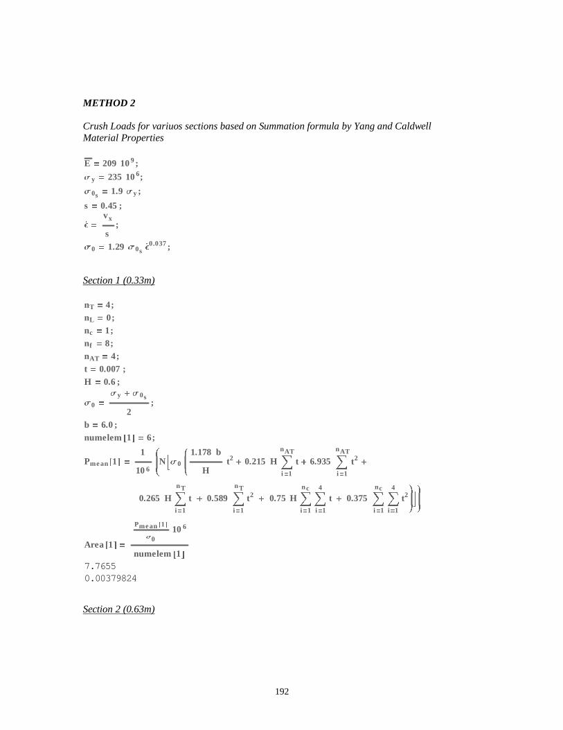
192
METHOD 2
Crush Loads for variuos sections based on Summation formula by Yang and CaldwellMaterial Properties
E 209 109;
Vy 235 106;
V0s 1.9 Vy ;
s 0.45 ;
H�
vx
s;
V0 1.29 V0s H� 0.037;
Section 1 (0.33m)
nT 4;nL 0;nc 1;nf 8;nAT 4;t 0.007 ;H 0.6 ;
V0 Vy � V0s
2;
b 6.0 ;numelem#1' 6;
Pmean#1' 1
106
L
N
N%V0
L
N
1.178 b
Ht2� 0.215 HÅ
i 1
nAT
t � 6.935 Åi 1
nAT
t2�
0.265 HÅi 1
nT
t � 0.589Åi 1
nT
t2� 0.75 HÅ
i 1
nc
Åi 1
4
t � 0.375Åi 1
nc
Åi 1
4
t2\
^)\
^
Area #1'
Pmean#1'
V0106
numelem#1'
7.76550.00379824
Section 2 (0.63m)
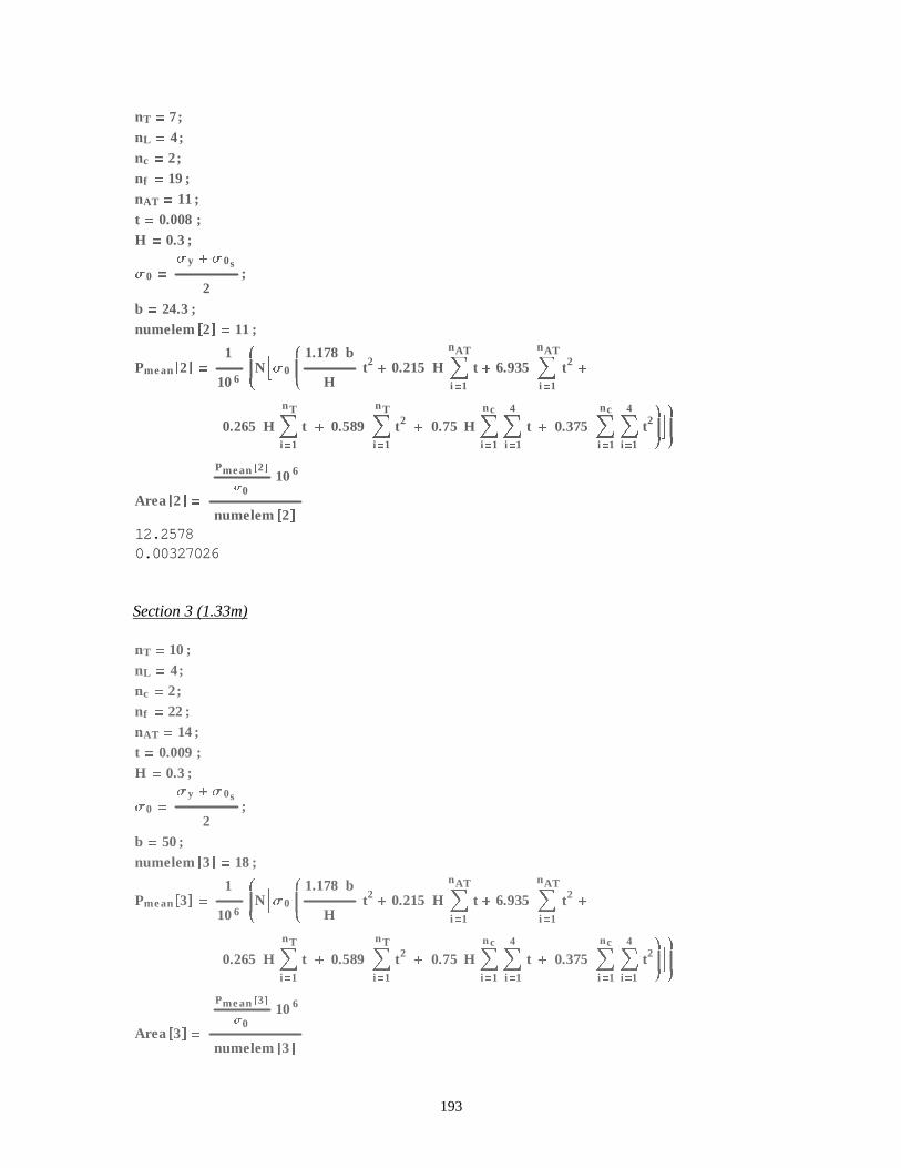
193
nT 7;nL 4;nc 2;nf 19 ;nAT 11 ;t 0.008 ;H 0.3 ;
V0 Vy � V0s
2;
b 24.3 ;numelem#2' 11 ;
Pmean#2' 1
106
L
NN%V0
L
N
1.178 b
Ht2� 0.215 HÅ
i 1
nAT
t � 6.935 Åi 1
nAT
t2�
0.265 HÅi 1
nT
t � 0.589Åi 1
nT
t2� 0.75 HÅ
i 1
nc
Åi 1
4
t � 0.375Åi 1
nc
Åi 1
4
t2\
^)\
^
Area #2'
Pmean#2'
V0106
numelem#2'
12.25780.00327026
Section 3 (1.33m)
nT 10 ;nL 4;nc 2;nf 22 ;nAT 14 ;t 0.009 ;H 0.3 ;
V0 Vy � V0s
2;
b 50 ;numelem#3' 18 ;
Pmean#3' 1
106
L
NN%V0
L
N
1.178 b
Ht2� 0.215 HÅ
i 1
nAT
t � 6.935 Åi 1
nAT
t2�
0.265 HÅi 1
nT
t � 0.589Åi 1
nT
t2� 0.75 HÅ
i 1
nc
Åi 1
4
t � 0.375Åi 1
nc
Åi 1
4
t2\
^)\
^
Area #3'
Pmean#3'
V0106
numelem#3'
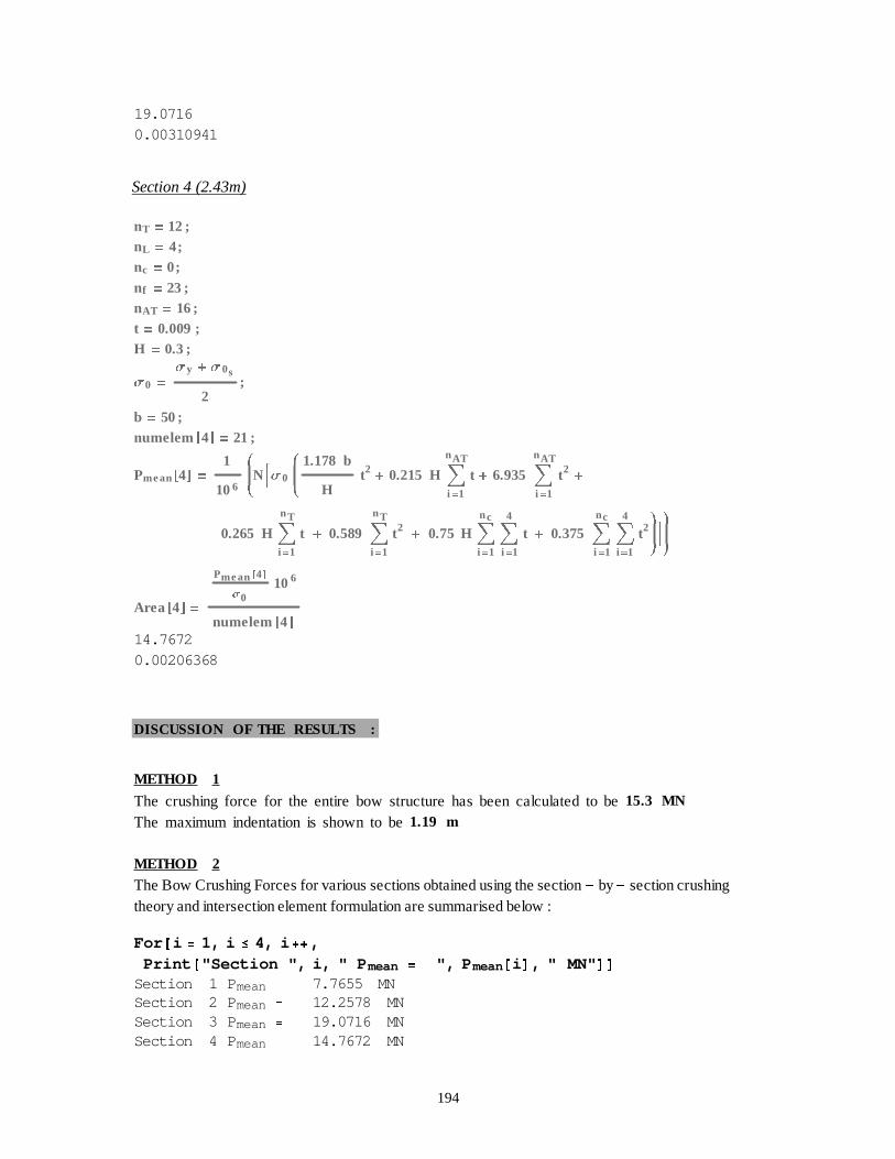
194
19.07160.00310941
Section 4 (2.43m)
nT 12 ;nL 4;nc 0;nf 23 ;nAT 16 ;t 0.009 ;H 0.3 ;
V0 Vy � V0s
2;
b 50 ;numelem#4' 21 ;
Pmean#4' 1
106
L
NN%V0
L
N
1.178 b
Ht2� 0.215 HÅ
i 1
nAT
t � 6.935 Åi 1
nAT
t2�
0.265 HÅi 1
nT
t � 0.589Åi 1
nT
t2� 0.75 HÅ
i 1
nc
Åi 1
4
t � 0.375Åi 1
nc
Åi 1
4
t2\
^)\
^
Area #4'
Pmean#4'
V0106
numelem#4'
14.76720.00206368
DISCUSSION OF THE RESULTS :
METHOD 1
The crushing force for the entire bow structure has been calculated to be15.3 MN
The maximum indentation is shown to be1.19 m
METHOD 2
The Bow Crushing Forces for various sections obtained using the section� by� section crushingtheory and intersection element formulation are summarised below :
For #i 1, i � 4, i �� ,Print #"Section ", i, " P mean ", P mean#i ', " MN" ''
Section 1 P mean 7.7655 MNSection 2 P mean 12.2578 MNSection 3 P mean 19.0716 MNSection 4 P mean 14.7672 MN
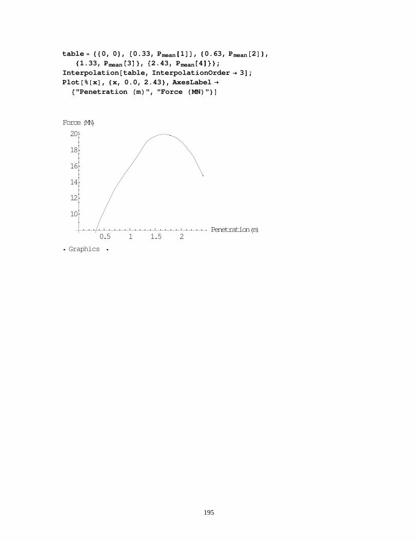
195
table ��0, 0 �, �0.33, P mean#1'�, �0.63, P mean#2'�,�1.33, P mean#3'�, �2.43, P mean#4'��;
Interpolation #table, InterpolationOrder � 3';Plot #%#x', �x, 0.0, 2.43 �, AxesLabel �
�"Penetration +m/", "Force +MN/" �'
0.5 1 1.5 2Penetration +m/
10
12
14
16
18
20
Force +MN/
h Graphics h

196
23, 000 DWT Containership :Ship ParticularsLBP 220.91 ;
B 26.01 ;
dMLD 16.11 ;
d 9.684 ;
T 9.70 ;' 31050 ;
Vservice 11.32 ;
vx Vservice;
METHOD 1
Regression-based Crushing load and location of maximum indentationCalculations based on ship particulars
L LBP s 275 ;
mx 1.05 '
1000;
V0 Vservice;
KE
1
2' V0
2 1000 ;
Eimp 1
2mx V0
2;
Eimp Eimp s 1425 ;
P0 210 ;
If $Eimp ! L 2.6, Pbow P0 L , Eimp � ,5.0 � L 0 L 1.600.5(;
If $Eimp � L 2.6, Pbow 2.24 P0 ,Eimp L 00.5(;
Print #"Kinetic Energy ", KE s 106 MJ ';Print #"Crush Load ", P bow MN ';
smax S
2
Eimp
Pbow
metres ;
Print #"Maximum indentation ", s max';
Kinetic Energy 1989.41 MJCrush Load 354.74 MNMaximum indentation 9.2496 metres
METHOD 2Crush Loads for various sections based on Summation formula by Yang and CaldwellMaterial Properties
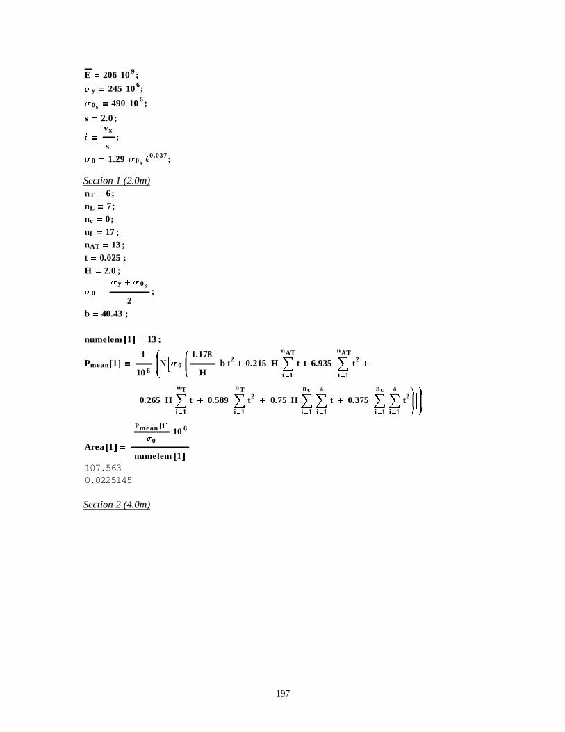
197
E 206 109;
Vy 245 106;
V0s 490 106;
s 2.0 ;
H�
vx
s;
V0 1.29 V0s H� 0.037;
Section 1 (2.0m)nT 6;nL 7;nc 0;nf 17 ;nAT 13 ;t 0.025 ;H 2.0 ;
V0 Vy � V0s
2;
b 40.43 ;
numelem#1' 13 ;
Pmean#1' 1
106
L
N
N%V0
L
N
1.178
Hb t2
� 0.215 HÅi 1
nAT
t � 6.935 Åi 1
nAT
t2�
0.265 HÅi 1
nT
t � 0.589Åi 1
nT
t2� 0.75 HÅ
i 1
nc
Åi 1
4
t � 0.375Åi 1
nc
Åi 1
4
t2\
^)\
^
Area #1'
Pmean#1'
V0106
numelem#1'
107.5630.0225145
Section 2 (4.0m)
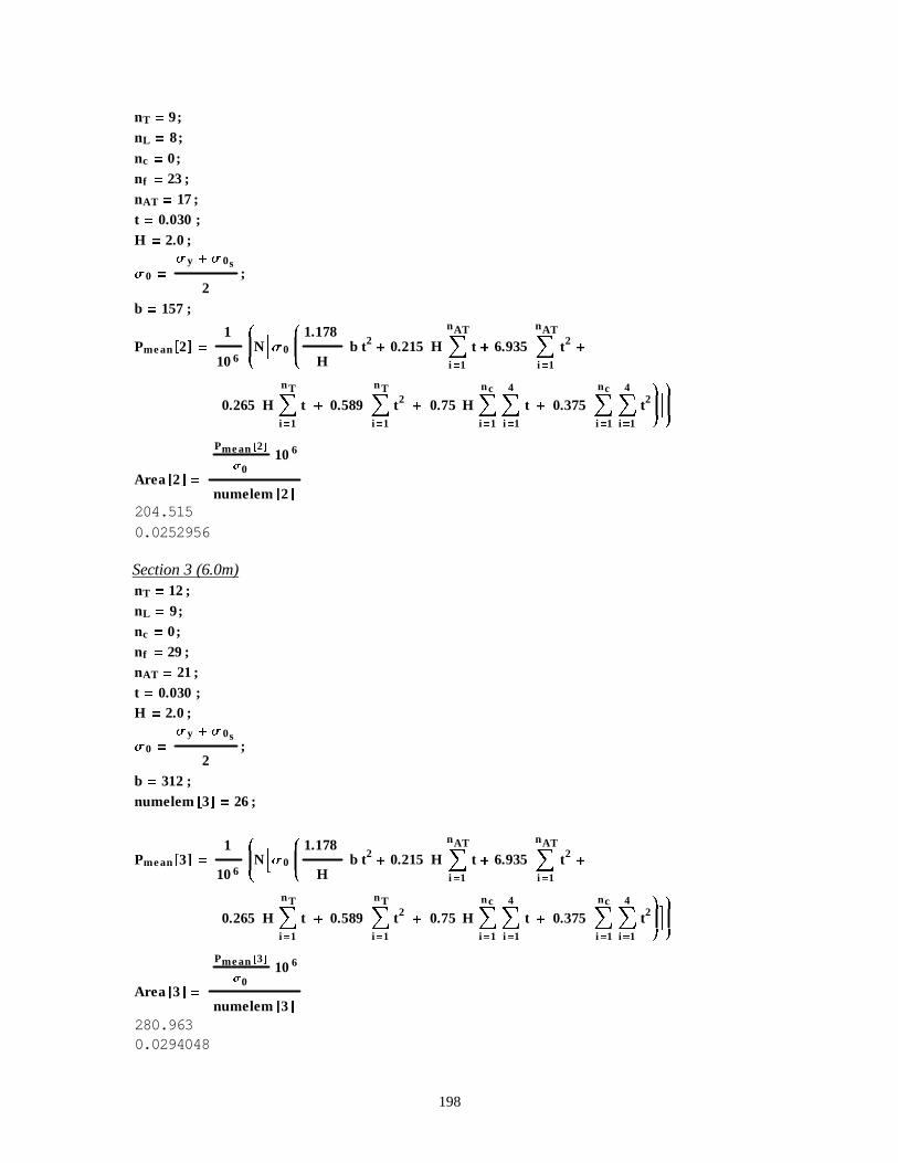
198
nT 9;nL 8;nc 0;nf 23 ;nAT 17 ;t 0.030 ;H 2.0 ;
V0 Vy � V0s
2;
b 157 ;
Pmean#2' 1
106
L
NN%V0
L
N
1.178
Hb t2
� 0.215 HÅi 1
nAT
t � 6.935 Åi 1
nAT
t2�
0.265 HÅi 1
nT
t � 0.589Åi 1
nT
t2� 0.75 HÅ
i 1
nc
Åi 1
4
t � 0.375Åi 1
nc
Åi 1
4
t2\
^)\
^
Area #2'
Pmean#2'
V0106
numelem#2'204.5150.0252956
Section 3 (6.0m)nT 12 ;nL 9;nc 0;nf 29 ;nAT 21 ;t 0.030 ;H 2.0 ;
V0 Vy � V0s
2;
b 312 ;numelem#3' 26 ;
Pmean#3' 1
106
L
NN%V0
L
N
1.178
Hb t2
� 0.215 HÅi 1
nAT
t � 6.935 Åi 1
nAT
t2�
0.265 HÅi 1
nT
t � 0.589Åi 1
nT
t2� 0.75 HÅ
i 1
nc
Åi 1
4
t � 0.375Åi 1
nc
Åi 1
4
t2\
^)\
^
Area #3'
Pmean#3'
V0106
numelem#3'
280.9630.0294048
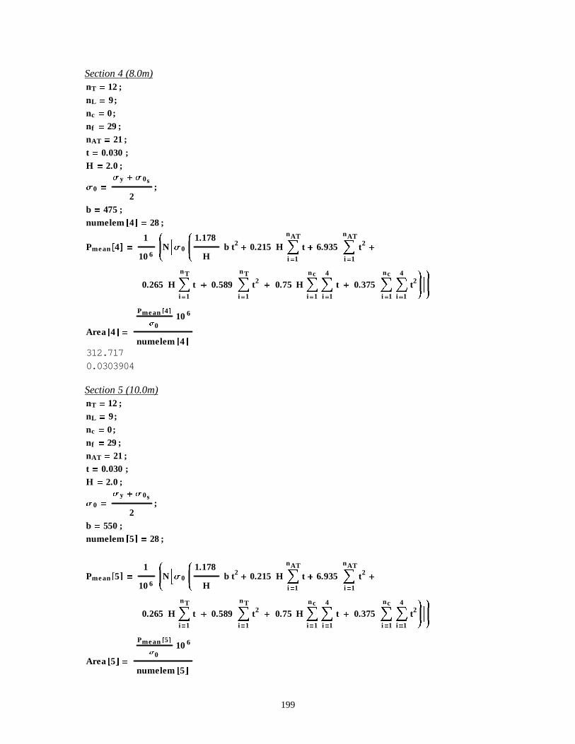
199
Section 4 (8.0m)nT 12 ;nL 9;nc 0;nf 29 ;nAT 21 ;t 0.030 ;H 2.0 ;
V0 Vy � V0s
2;
b 475 ;numelem#4' 28 ;
Pmean#4' 1
106
L
NN%V0
L
N
1.178
Hb t2
� 0.215 HÅi 1
nAT
t � 6.935 Åi 1
nAT
t2�
0.265 HÅi 1
nT
t � 0.589Åi 1
nT
t2� 0.75 HÅ
i 1
nc
Åi 1
4
t � 0.375Åi 1
nc
Åi 1
4
t2\
^)\
^
Area #4'
Pmean#4'
V0106
numelem#4'312.7170.0303904
Section 5 (10.0m)nT 12 ;nL 9;nc 0;nf 29 ;nAT 21 ;t 0.030 ;H 2.0 ;
V0 Vy � V0s
2;
b 550 ;numelem#5' 28 ;
Pmean#5' 1
106
L
NN%V0
L
N
1.178
Hb t2
� 0.215 HÅi 1
nAT
t � 6.935 Åi 1
nAT
t2�
0.265 HÅi 1
nT
t � 0.589Åi 1
nT
t2� 0.75 HÅ
i 1
nc
Åi 1
4
t � 0.375Åi 1
nc
Åi 1
4
t2\
^)\
^
Area #5'
Pmean#5'
V0106
numelem#5'
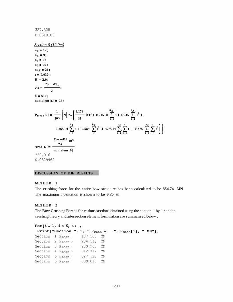
200
327.3280.0318103
Section 6 (12.0m)nT 12 ;nL 9;
nc 0;
nf 29 ;nAT 21 ;
t 0.030 ;
H 2.0 ;
V0 Vy � V0s
2;
b 610 ;numelem#6' 28 ;
Pmean#6' 1
106
L
NN%V0
L
N
1.178
Hb t2
� 0.215 HÅi 1
nAT
t � 6.935Åi 1
nAT
t2�
0.265 HÅi 1
nT
t � 0.589Åi 1
nT
t2� 0.75 HÅ
i 1
nc
Åi 1
4
t � 0.375Åi 1
nc
Åi 1
4
t2\
^)\
^
Area #6'
Pmean#6'
V0106
numelem#6'
339.0160.0329462
DISCUSSION OF THE RESULTS :
METHOD 1
The crushing force for the entire bow structure has been calculated to be354.74 MN
The maximum indentation is shown to be9.25 m
METHOD 2
The Bow Crushing Forces for various sections obtained using the section� by� sectioncrushing theory and intersection element formulation are summarised below :
For #i 1, i � 6, i �� ,Print #"Section ", i, " P mean ", P mean#i ', " MN" ''
Section 1 P mean 107.563 MNSection 2 P mean 204.515 MNSection 3 P mean 280.963 MNSection 4 P mean 312.717 MNSection 5 P mean 327.328 MNSection 6 P mean 339.016 MN
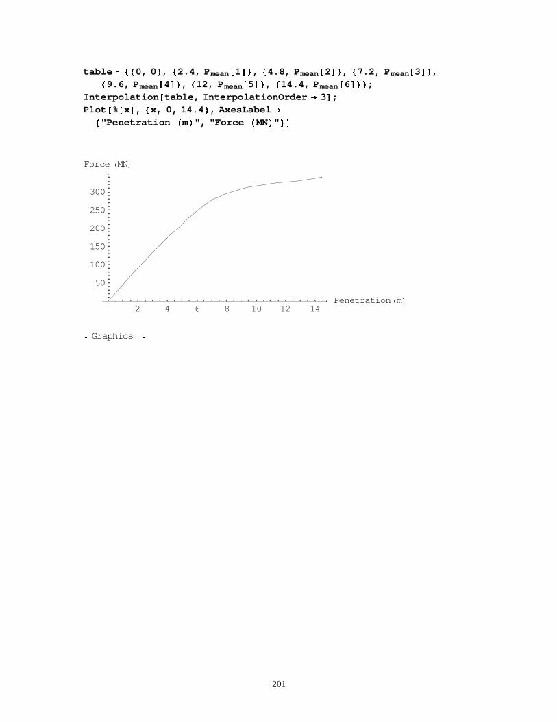
201
table ��0, 0 �, �2.4, P mean#1'�, �4.8, P mean#2'�, �7.2, P mean#3'�,�9.6, P mean#4'�, �12, P mean#5'�, �14.4, P mean#6'��;
Interpolation #table, InterpolationOrder � 3';Plot #%#x', �x, 0, 14.4 �, AxesLabel �
�"Penetration +m/", "Force +MN/" �'
2 4 6 8 10 12 14Penetration +m/
50
100
150
200
250
300
Force +MN/
h Graphics h

202
40, 000 DWT Containership :
Ship Particulars
LBP 211.50 ;B 32.20 ;dMLD 21.00 ;d 24.00 ;T 11.90 ;' 54000 ;Vservice 12.90 ;vx Vservice;
METHOD 1
Regression-based Crushing load and location of maximum indentationCalculations based on ship particulars
L LBP s 275 ;
mx 1.05 '
1000;
V0 Vservice;
KE
1
2' V0
2 1000 ;
Eimp 1
2mx V0
2;
Eimp Eimp s 1425 ;
P0 210 ;
If $Eimp ! L 2.6, Pbow P0 L , Eimp � ,5.0 � L 0 L 1.600.5
(;
If $Eimp � L 2.6, Pbow 2.24 P0 ,Eimp L 00.5(;
Print #"Kinetic Energy ", KE s 106 MJ ';Print #"Crush Load ", P bow MN ';
smax S
2
Eimp
Pbow
metres ;
Print #"Maximum indentation ", s max';
Kinetic Energy 4493.07 MJCrush Load 398.583 MNMaximum indentation 18.5923 metres
METHOD 2
Crush Loads for variuos sections based on Summation formula by Yang and CaldwellMaterial Properties
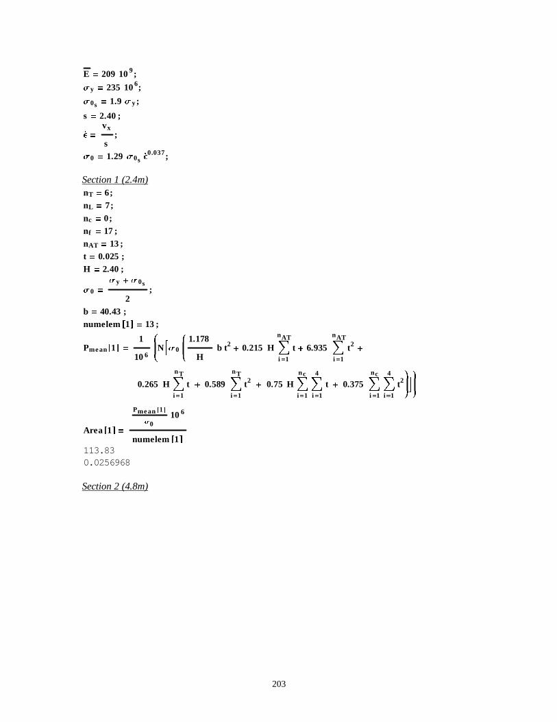
203
E 209 109;
Vy 235 106;
V0s 1.9 Vy ;
s 2.40 ;
H�
vx
s;
V0 1.29 V0s H� 0.037;
Section 1 (2.4m)nT 6;nL 7;nc 0;nf 17 ;nAT 13 ;t 0.025 ;H 2.40 ;
V0 Vy � V0s
2;
b 40.43 ;numelem#1' 13 ;
Pmean#1' 1
106
L
NN%V0
L
N
1.178
Hb t2
� 0.215 HÅi 1
nAT
t � 6.935 Åi 1
nAT
t2�
0.265 HÅi 1
nT
t � 0.589Åi 1
nT
t2� 0.75 HÅ
i 1
nc
Åi 1
4
t � 0.375Åi 1
nc
Åi 1
4
t2\
^)\
^
Area #1'
Pmean#1'
V0106
numelem#1'
113.830.0256968
Section 2 (4.8m)
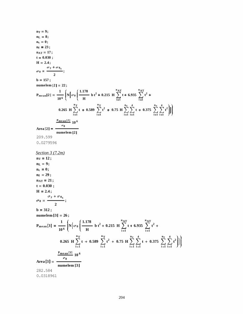
204
nT 9;
nL 8;nc 0;
nf 23 ;
nAT 17 ;
t 0.030 ;H 2.4 ;
V0
Vy � V0s
2;
b 157 ;
numelem#2' 22 ;
Pme an#2' 1
106
L
N
N%V0
L
N
1.178
Hb t2
� 0.215 HÅi 1
nAT
t � 6.935Åi 1
nAT
t2�
0.265 HÅi 1
nT
t � 0.589Åi 1
nT
t2� 0.75 HÅ
i 1
nc
Åi 1
4
t � 0.375Åi 1
nc
Åi 1
4
t2\
^)\
^
Area #2'
Pme an#2'
V0106
numelem#2'
209.5990.0279596
Section 3 (7.2m)nT 12 ;nL 9;nc 0;nf 29 ;nAT 21 ;t 0.030 ;H 2.4 ;
V0
Vy � V0s
2;
b 312 ;numelem#3' 26 ;
Pmean#3' 1
106
L
NN%V0
L
N
1.178
Hb t2
� 0.215 HÅi 1
nAT
t � 6.935 Åi 1
nAT
t2�
0.265 HÅi 1
nT
t � 0.589Åi 1
nT
t2� 0.75 HÅ
i 1
nc
Åi 1
4
t � 0.375Åi 1
nc
Åi 1
4
t2\
^)\
^
Area #3'
Pmean#3'
V0106
numelem#3'
282.5840.0318961
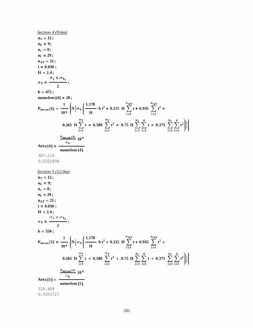
205
Section 4 (9.6m)nT 12 ;nL 9;nc 0;nf 29 ;nAT 21 ;t 0.030 ;H 2.4 ;
V0
Vy � V0s
2;
b 475 ;numelem#4' 28 ;
Pmean#4' 1
106
L
N
N%V0
L
N
1.178
Hb t2
� 0.215 HÅi 1
nAT
t � 6.935 Åi 1
nAT
t2�
0.265 HÅi 1
nT
t � 0.589Åi 1
nT
t2� 0.75 HÅ
i 1
nc
Åi 1
4
t � 0.375Åi 1
nc
Åi 1
4
t2\
^)\
^
Area #4'
Pmean#4'
V0106
numelem#4'
307.1190.0321894
Section 5 (12.0m)nT 12 ;nL 9;nc 0;nf 29 ;nAT 21 ;t 0.030 ;H 2.4 ;
V0
Vy � V0s
2;
b 550 ;
Pmean#5' 1
106
L
N
N%V0
L
N
1.178
Hb t2
� 0.215 HÅi 1
nAT
t � 6.935 Åi 1
nAT
t2�
0.265 HÅi 1
nT
t � 0.589Åi 1
nT
t2� 0.75 HÅ
i 1
nc
Åi 1
4
t � 0.375Åi 1
nc
Åi 1
4
t2\
^)\
^
Area #5'
Pmean#5'
V0106
numelem#5'
318.4090.0333727
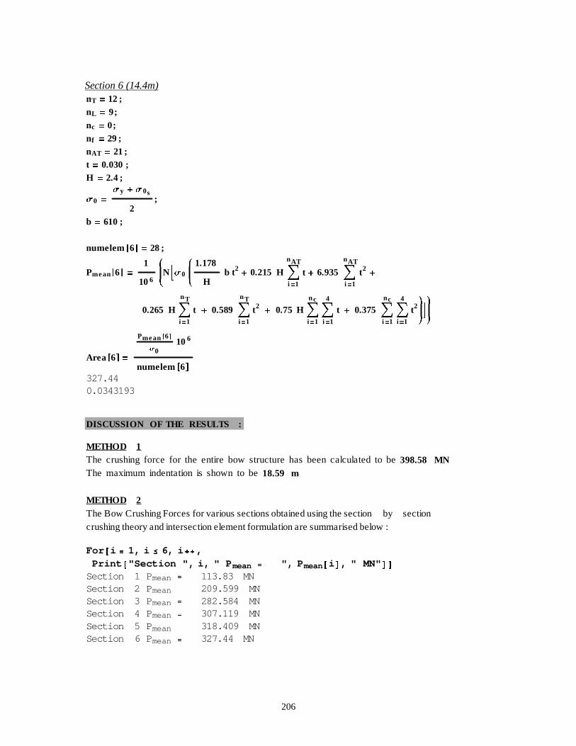
206
Section 6 (14.4m)nT 12 ;nL 9;nc 0;nf 29 ;nAT 21 ;t 0.030 ;H 2.4 ;
V0 Vy � V0s
2;
b 610 ;
numelem#6' 28 ;
Pmean#6' 1
106
L
NN%V0
L
N
1.178
Hb t2
� 0.215 HÅi 1
nAT
t � 6.935 Åi 1
nAT
t2�
0.265 HÅi 1
nT
t � 0.589Åi 1
nT
t2� 0.75 HÅ
i 1
nc
Åi 1
4
t � 0.375Åi 1
nc
Åi 1
4
t2\
^)\
^
Area #6'
Pmean#6'
V0106
numelem#6'
327.440.0343193
DISCUSSION OF THE RESULTS :
METHOD 1The crushing force for the entire bow structure has been calculated to be398.58 MNThe maximum indentation is shown to be18.59 m
METHOD 2The Bow Crushing Forces for various sections obtained using the section
�by�
sectioncrushing theory and intersection element formulation are summarised below :
For #i 1, i � 6, i �� ,Print #"Section ", i, " P mean ", P mean#i ', " MN" ''
Section 1 P mean 113.83 MNSection 2 P mean 209.599 MNSection 3 P mean 282.584 MNSection 4 P mean 307.119 MNSection 5 P mean 318.409 MNSection 6 P mean 327.44 MN
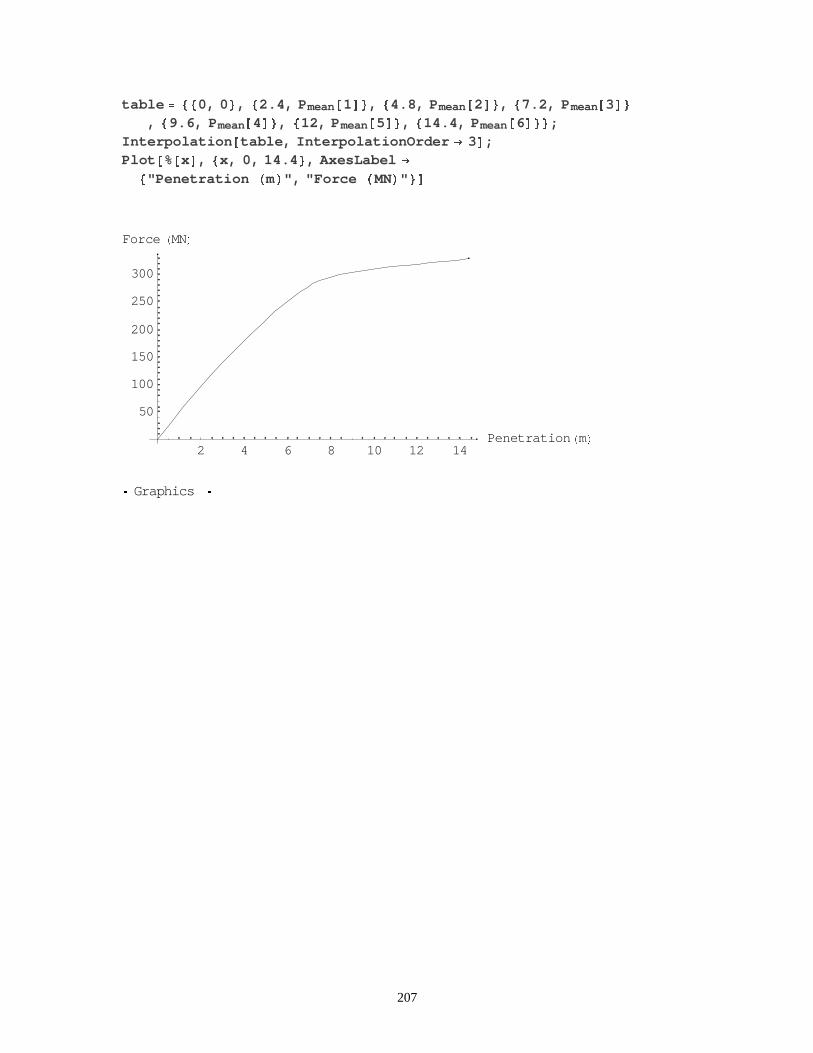
207
table ��0, 0 �, �2.4, P mean#1'�, �4.8, P mean#2'�, �7.2, P mean#3'�, �9.6, P mean#4'�, �12, P mean#5'�, �14.4, P mean#6'��;
Interpolation #table, InterpolationOrder � 3';Plot #%#x', �x, 0, 14.4 �, AxesLabel �
�"Penetration +m/", "Force +MN/" �'
2 4 6 8 10 12 14Penetration +m/
50
100
150
200
250
300
Force +MN/
h Graphics h

208
150, 000 DWT Bulk Carrier :Ship Particulars
LBP 274.50 ;B 47.00 ;dMLD 21.60 ;d 26.00 ;T 15.96 ;' 174850 ;Vservice 9.3 ;vx Vservice;
METHOD 1
Regression-based Crushing load and location of maximum indentation Calculations based onship particulars
L LBP s 275 ;
mx 1.05 '
1000;
V0 Vservice;
Eimp 1
2mx V0
2;
KE
1
2' V0
2 1000 ;
Eimp Eimp s 1425 ;
P0 210 ;
If $Eimp ! L2.6
, Pbow P0 L , Eimp � ,5.0 � L 0 L1.6
00.5
(;
If $Eimp � L2.6
, Pbow 2.24 P0 ,Eimp L 00.5(;
Print #"Kinetic Energy ", KE s 106 MJ ';Print #"Crush Load ", P bow MN ';
smax S
2
Eimp
Pbow
metres ;
Print #"Maximum indentation ", s max';
Kinetic Energy 7561.39 MJCrush Load 648.182 MNMaximum indentation 19.2404 metres
METHOD 2
Crush Loads for variuos sections based on Summation formula by Yang and CaldwellMaterial Properties
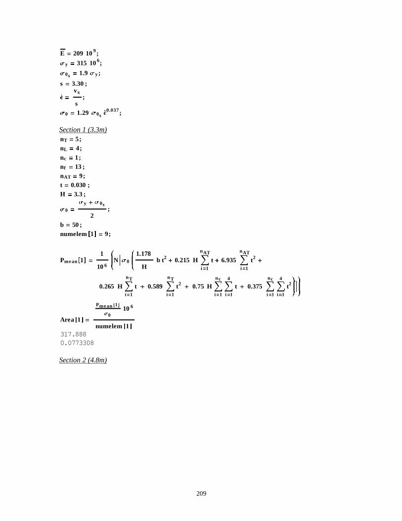
209
E 209 109;
Vy 315 106;
V0s 1.9 Vy ;
s 3.30 ;
H�
vx
s;
V0 1.29 V0s H� 0.037;
Section 1 (3.3m)nT 5;nL 4;nc 1;nf 13 ;nAT 9;t 0.030 ;H 3.3 ;
V0 Vy � V0s
2;
b 50 ;numelem#1' 9;
Pmean#1' 1
106
L
NN%V0
L
N
1.178
Hb t2
� 0.215 HÅi 1
nAT
t � 6.935 Åi 1
nAT
t2�
0.265 HÅi 1
nT
t � 0.589Åi 1
nT
t2� 0.75 HÅ
i 1
nc
Åi 1
4
t � 0.375Åi 1
nc
Åi 1
4
t2\
^)\
^
Area #1'
Pmean#1'
V0106
numelem#1'
317.8880.0773308
Section 2 (4.8m)
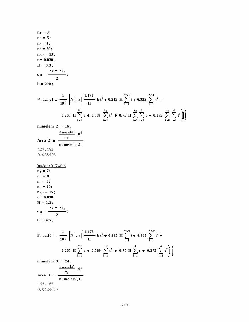
210
nT 8;nL 5;nc 1;nf 20 ;nAT 13 ;t 0.030 ;H 3.3 ;
V0 Vy � V 0s
2;
b 200 ;
Pme an#2' 1
106
L
NN%V0
L
N
1.178
Hb t2
� 0.215 HÅi 1
nAT
t � 6.935 Åi 1
nAT
t2�
0.265 HÅi 1
n T
t � 0.589 Åi 1
n T
t2� 0.75 HÅ
i 1
n c
Åi 1
4
t � 0.375 Åi 0
nc
Åi 1
4
t2\
^)\
^numelem#2' 16 ;
Area #2'
Pme an#2'
V0106
numelem#2'
427.4810.058495
Section 3 (7.2m)nT 7 ;
nL 8 ;nc 0;nf 20 ;
nAT 15 ;t 0.030 ;H 3.3 ;
V 0 V y � V 0s
2;
b 375 ;
Pm e an#3' 1
106
L
NN %V 0
L
N
1.178
Hb t2
� 0.215 H Åi 1
nAT
t � 6.935 Åi 1
n AT
t2�
0.265 HÅi 1
nT
t � 0.589 Åi 1
n T
t2� 0.75 HÅ
i 1
4
t � 0.375 Åi 1
4
t2\
^)\
^numelem#3' 24 ;
Area #3'
Pm e an #3'
V0106
numelem#3'
465.4650.0424617
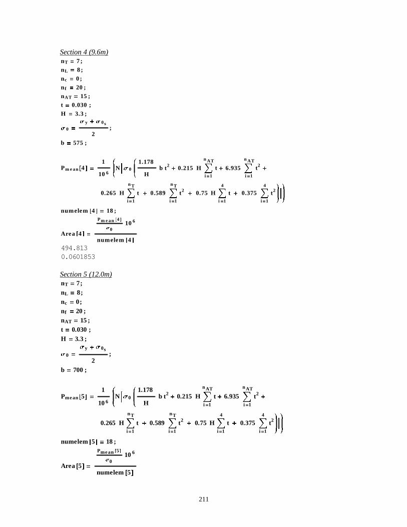
211
Section 4 (9.6m)nT 7 ;
nL 8 ;
nc 0 ;
nf 20 ;
nAT 15 ;
t 0.030 ;
H 3.3 ;
V 0
V y � V 0s
2;
b 575 ;
Pm e an#4' 1
106
L
NN %V 0
L
N
1.178
Hb t2
� 0.215 H Åi 1
n AT
t � 6.935 Åi 1
n AT
t2�
0.265 HÅi 1
n T
t � 0.589 Åi 1
n T
t2� 0.75 HÅ
i 1
4
t � 0.375 Åi 1
4
t 2\
^)\
^numelem#4' 18 ;
Area #4'
Pm e an#4'
V0106
numelem#4'
494.8130.0601853
Section 5 (12.0m)nT 7;nL 8;nc 0;nf 20 ;nAT 15 ;t 0.030 ;H 3.3 ;
V0 Vy � V0s
2;
b 700 ;
Pmean#5' 1
106
L
N
N%V0
L
N
1.178
Hb t2
� 0.215 HÅi 1
nAT
t � 6.935Åi 1
nAT
t2�
0.265 HÅi 1
nT
t � 0.589Åi 1
nT
t2� 0.75 HÅ
i 1
4
t � 0.375Åi 1
4
t2\
^)\
^numelem#5' 18 ;
Area #5'
Pmean#5'
V0106
numelem#5'
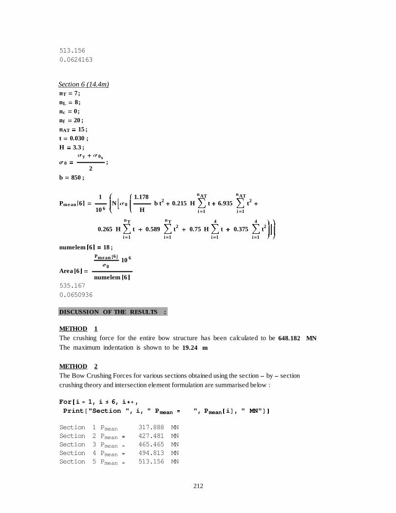
212
513.1560.0624163
Section 6 (14.4m)nT 7;nL 8;nc 0;nf 20 ;nAT 15 ;t 0.030 ;H 3.3 ;
V0 Vy � V0s
2;
b 850 ;
Pmean#6' 1
106
L
NN%V0
L
N
1.178
Hb t2
� 0.215 HÅi 1
nAT
t � 6.935Åi 1
nAT
t2�
0.265 HÅi 1
nT
t � 0.589Åi 1
nT
t2� 0.75 HÅ
i 1
4
t � 0.375Åi 1
4
t2\
^)\
^numelem#6' 18 ;
Area #6'
Pmean#6'
V0106
numelem#6'
535.1670.0650936
DISCUSSION OF THE RESULTS :
METHOD 1The crushing force for the entire bow structure has been calculated to be648.182 MNThe maximum indentation is shown to be19.24 m
METHOD 2The Bow Crushing Forces for various sections obtained using the section� by� sectioncrushing theory and intersection element formulation are summarised below :
For #i 1, i � 6, i �� ,Print #"Section ", i, " P mean ", P mean#i ', " MN" ''
Section 1 P mean 317.888 MNSection 2 P mean 427.481 MNSection 3 P mean 465.465 MNSection 4 P mean 494.813 MNSection 5 P mean 513.156 MN
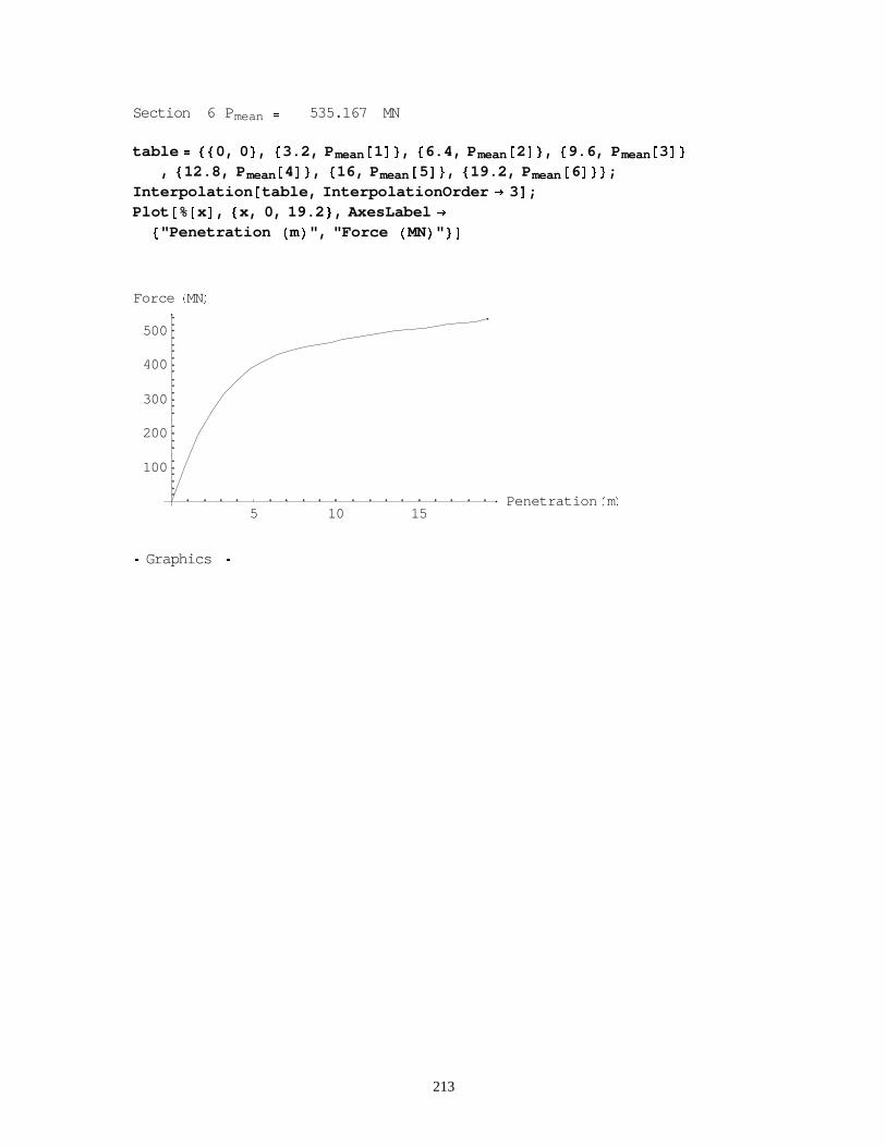
213
Section 6 P mean 535.167 MN
table ��0, 0 �, �3.2, P mean#1'�, �6.4, P mean#2'�, �9.6, P mean#3'�, �12.8, P mean#4'�, �16, P mean#5'�, �19.2, P mean#6'��;
Interpolation #table, InterpolationOrder � 3';Plot #%#x', �x, 0, 19.2 �, AxesLabel �
�"Penetration +m/", "Force +MN/" �'
5 10 15Penetration +m/
100
200
300
400
500
Force +MN/
h Graphics h
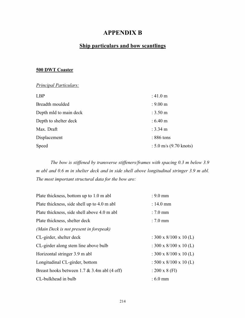
214
APPENDIX B
Ship particulars and bow scantlings
500 DWT Coaster
Principal Particulars:
LBP : 41.0 m
Breadth moulded : 9.00 m
Depth mld to main deck : 3.50 m
Depth to shelter deck : 6.40 m
Max. Draft : 3.34 m
Displacement : 886 tons
Speed : 5.0 m/s (9.70 knots)
The bow is stiffened by transverse stiffeners/frames with spacing 0.3 m below 3.9
m abl and 0.6 m in shelter deck and in side shell above longitudinal stringer 3.9 m abl.
The most important structural data for the bow are:
Plate thickness, bottom up to 1.0 m abl : 9.0 mm
Plate thickness, side shell up to 4.0 m abl : 14.0 mm
Plate thickness, side shell above 4.0 m abl : 7.0 mm
Plate thickness, shelter deck : 7.0 mm
(Main Deck is not present in forepeak)
CL-girder, shelter deck : 300 x 8/100 x 10 (L)
CL-girder along stem line above bulb : 300 x 8/100 x 10 (L)
Horizontal stringer 3.9 m abl : 300 x 8/100 x 10 (L)
Longitudinal CL-girder, bottom : 500 x 8/100 x 10 (L)
Breast hooks between 1.7 & 3.4m abl (4 off) : 200 x 8 (Fl)
CL-bulkhead in bulb : 6.0 mm

215
23,000 DWT Containership
Principal dimensions:
LBP : 211.50 m
Breadth moulded : 32.20 m
Depth mld to main deck : 21.00 m
Depth to shelter deck : 24.00 m
Max. Draft : 11.90 m
Displacement (Loaded) : 54,000 tons
Max. Service Speed : 11.3 m/s (21.97 knots)
The bulbous bow is stiffened longitudinally. The transverse frames supporting the
longitudinals have a spacing of 2.4 m. The most important structural data for the bow
are:
Bottom:
Plate thickness : 19.0 mm
Longitudinals, spacing 0.8 m : L 250 X 90 X 12 / 16
CL-Girder : L 1900 X 250 X 15 / 25
Side shell:
Plate thickness, side shell up to 6.1 m abl : 17.0 mm
Plate thickness, side shell between 6.1 and 12.3 m abl : 35.0 mm
Plate thickness, side shell between 12.3 and 21.0 m abl : 16.0 mm
Plate thickness, side shell above 21.0 m abl : 14.0 mm
Longitudinals below 5.2 m abl and above 13.6 m abl : L250 x 90 x 10/15
(spacing 0.8 m)
Longitudinals between 6.6 and 12.0 m abl, spacing 0.6 m : L250 x 90 x 12/16
Forecastle deck, 24.0 m abl
216
Plate thickness : 15.0 mm
Longitudinals, spacing 0.8 m : L150 x 100 x 9
CL-girder : L700 x 150 x 12/12
Main deck,21.0 m abl
Plate thickness : 11.0 mm
Longitudinals, spacing 0.8 m : L150 x 100 x 9
CL-girder : L700 x 150 x 12/12
Deck 17.6 m abl
Plate thickness : 11.0 mm
Longitudinals, spacing 0.8 m : L150 x 100 x 9
CL-girder : L700 x 150 x 12/12
Deck 12.8 m abl
Plate thickness : 15.0 mm
Longitudinals, spacing 0.8 m : L200 x 90 x 9/14
CL-girder : L700 x 150 x 12/12
Deck (not water-tight), 6 m abl
Plate thickness : 11.0 mm
Longitudinals, spacing 0.8 m : Fl. 150 x 12

217
40,000 DWT Containership
Principal dimensions:
LBP : 211.50 m
Breadth moulded : 32.20 m
Depth mld to main deck : 21.00 m
Depth to shelter deck : 24.00 m
Max. Draft : 11.90 m
Displacement (Loaded) : 54,000 tons
Max. Service Speed : 11.3 m/s (21.97 knots)
The bulbous bow is stiffened longitudinally. The transverse frames supporting the
longitudinals have a spacing of 2.4 m. The most important structural data for the bow
are:
Bottom:
Plate thickness : 19.0 mm
Longitudinals, spacing 0.8 m : L 250 X 90 X 12 / 16
CL-Girder : L 1900 X 250 X 15 / 25
Side shell
Plate thickness, side shell up to 6.1 m abl : 17.0 mm
Plate thickness, side shell between 6.1 and 12.3 m abl : 35.0 mm
Plate thickness, side shell between 12.3 and 21.0 m abl : 16.0 mm
Plate thickness, side shell above 21.0 m abl : 14.0 mm
Longitudinals below 5.2 m abl and above 13.6 m abl : L250 x 90 x 10/15
(spacing 0.8 m)
Longitudinals between 6.6 and 12.0 m abl, spacing 0.6 m : L250 x 90 x 12/16
Forecastle deck, 24.0 m abl

218
Plate thickness : 15.0 mm
Longitudinals, spacing 0.8 m : L150 x 100 x 9
CL-girder : L700 x 150 x 12/12
Main deck,21.0 m abl
Plate thickness : 11.0 mm
Longitudinals, spacing 0.8 m : L150 x 100 x 9
CL-girder : L700 x 150 x 12/12
Deck 17.6 m abl
Plate thickness : 11.0 mm
Longitudinals, spacing 0.8 m : L150 x 100 x 9
CL-girder : L700 x 150 x 12/12
Deck 12.8 m abl
Plate thickness : 15.0 mm
Longitudinals, spacing 0.8 m : L200 x 90 x 9/14
CL-girder : L700 x 150 x 12/12
Deck (not water-tight), 6 m abl
Plate thickness : 11.0 mm
Longitudinals, spacing 0.8 m : Fl. 150 x 12

219
150,000 DWT Bulk Carrier
Ship Particulars
LBP : 274 m
Breadth moulded : 47.0 m
Depth molded : 21.6 m
Depth to forecastle deck : 26.0 m
Max. Draft : 15.96 m
Displacement : 174850 tons
Max. service speed : 7.7 m/s ( 15.00 knots )
The bow is stiffened longitudinally. The transverse frames supporting the
longitudinals have a spacing of 3.2 m. The most important structural data for the bow
are:
Material
Yield Stress for plates and stiffeners (σY ) : 315 Mpa
Ratio between ultimate and Yield stress (σu/σY ) : 1.6
Bottom
plate thickness : 18.0 mm
longitudinals, spacing : L450 x 150 x 12/16
CL-Girder : L2500 x 400 x 15/25
Side shell
Plate thickness, side shell up to 8.1 m abl : 18.0 mm
Plate thickness, side shell between 8.1 and 17.0 m abl : 33.0 mm
Plate thickness, side shell between 17.0 and 26.0 m abl : 16.0 mm
Longitudinals between 1.2 and 6.8 m abl, spacing 0.8 m : L450 x 150 x 12/16
Longitudinals between 8.4 and 16.2 m abl, spacing 0.6 m : L400 x 100 x 19/19

220
Longitudinals between 17.4 and 24.8 m abl, spacing 0.8 m : L350 x 100 x 12/17
Forecastle deck, 26.0 m abl
Plate thickness : 13.0 mm
Longitudinals, spacing : L250 x 90 x 12/16
CL-girder : L1400 x 250 x 12/25
Tank top, 20.0 m abl
Plate thickness : 13.0 mm
Longitudinals, spacing : L250 x 90 x 12/16
CL-girder : L1400 x 250 x 12/25
Deck (not water-tight), 7.7 m abl
Plate thickness : 13.0 mm
Longitudinals, spacing : L250 x 90 x 12/16
CL-girder : L1400 x 250 x 12/25
Breast hooks
Number of breast hooks : 32
Cross-section : 1200 x 15
Length : 3000 mm
CL-girder along stem line cross-section : T1400 x 250 x 12/25
CL-bulkhead in bulb fwd F.P (plate thickness) : 12mm
Vertical stiffening spacing : 0.8 m

221
APPENDIX C
Example of an LS-DYNA input deck
*KEYWORD
$---+----1----+----2----+----3----+----4----+----5----+----6----+----7----+----8
$
$ DYNA3D(936) DECK WAS WRITTEN BY: ETA/FEMB VERSION 26
$ DATE : Nov 11, 1999 at 10:22:33
$ PREPARED BY: SURYANARAYANA VAKKALANKA (M.S)
$ AEROSPACE AND OCEAN ENGINEERING, VIRGINIA TECH.
$
$---+----1----+----2----+----3----+----4----+----5----+----6----+----7----+----8
$ (1) TITLE CARD.
$---+----1----+----2----+----3----+----4----+----5----+----6----+----7----+----8
*TITLE
150K SPEED12
$---+----1----+----2----+----3----+----4----+----5----+----6----+----7----+----8
$ (2) CONTROL CARDS.
$---+----1----+----2----+----3----+----4----+----5----+----6----+----7----+----8
*CONTROL_TERMINATION
$ ENDTIM ENDCYC DTMIN ENDNEG ENDMAS
.400E+01 0 .000 .000 .000
*CONTROL_TIMESTEP
$ DTINIT SCFT ISDO TSLIMT DTMS LCTM ERODE MS1ST
.000 .900 0
*CONTROL_HOURGLASS
$ IHQ QH
1 .100
222
*CONTROL_BULK_VISCOSITY
$ Q2 Q1
1.500 .060
*CONTROL_SHELL
$ WRPANG ITRIST IRNXX ISTUPD THEORY BWC MITER
20.000 2 -1 0 2 2 1
*CONTROL_CONTACT
$ SLSFAC RWPNAL ISLCHK SHLTHK PENOPT THKCHG ORIEN
.100
$ USRSTR USRFAC NSBCS INTERM XPENE
0 0 10 0 4.000
*CONTROL_ENERGY
$ HGEN RWEN SLNTEN RYLEN
1 2 1 1
*CONTROL_DAMPING
$ NRCYCK DRTOL DRFCTR DRTERM TSSFDR IRELAL EDTTL
IDRFLG
250 .001 .995
*CONTROL_OUTPUT
$ NPOPT NEECHO NREFUP IACCOP OPIFS IPNINT IKEDIT
0 0 0 0 .000 0 100
$---+----1----+----2----+----3----+----4----+----5----+----6----+----7----+----8
$ (3) DATABASE CONTROL CARDS - ASCII HISTORY FILE
$---+----1----+----2----+----3----+----4----+----5----+----6----+----7----+----8
$*DATABASE_HISTORY_OPTION
$ ID1 ID2 ID3 ID4 ID5 ID6 ID7 ID8
$
$OPTION : BEAM BEAM_SET NODE NODE_SET
$ SHELL SHELL_SET SOLID SOLID_SET
$ TSHELL TSHELL_SET
$---+----1----+----2----+----3----+----4----+----5----+----6----+----7----+----8
223
$ (4) DATABASE CONTROL CARDS FOR ASCII FILE
$---+----1----+----2----+----3----+----4----+----5----+----6----+----7----+----8
$---+----1----+----2----+----3----+----4----+----5----+----6----+----7----+----8
$*DATABASE_OPTION
$ DT
$
$OPTION : SECFORC RWFORC NODOUT ELOUT GLSTAT
$ DEFORC MATSUM NCFORC RCFORC DEFGEO
$ SPCFORC SWFORC ABSTAT NODFOR BNDOUT
$ RBDOUT GCEOUT SLEOUT MPGS SBTOUT
$ JNTFORC AVSFLT MOVIE
*DATABASE_GLSTAT
.800E-02
*DATABASE_RCFORC
.800E-02
$---+----1----+----2----+----3----+----4----+----5----+----6----+----7----+----8
$ (5) DATABASE CONTROL CARDS FOR BINARY FILE
$---+----1----+----2----+----3----+----4----+----5----+----6----+----7----+----8
*DATABASE_BINARY_D3PLOT
$ DT/CYCL LCDT NOBEAM
.200E+00
*DATABASE_BINARY_D3THDT
$ DT/CYCL LCDT NOBEAM
.200E+00
$*DATABASE_BINARY_OPTION
$ DT/CYCL LCDT NOBEAM
$
$OPTION : D3DRFL D3DUMP RUNRSF INTFOR
$---+----1----+----2----+----3----+----4----+----5----+----6----+----7----+----8
*DATABASE_EXTENT_BINARY
0 0 3 0 1 1 1 1
224
0 0 0 0 0 0
$---+----1----+----2----+----3----+----4----+----5----+----6----+----7----+----8
$ (6) DEFINE PARTS CARDS
$---+----1----+----2----+----3----+----4----+----5----+----6----+----7----+----8
*PART
$HEADING
PART PID = 8 PART NAME :TRANS
$ PID SID MID EOSID HGID GRAV ADPOPT TMID
8 8 4
*PART
$HEADING
PART PID = 1 PART NAME :WALL
$ PID SID MID EOSID HGID GRAV ADPOPT TMID
1 1 1
*PART
$HEADING
PART PID = 9 PART NAME :MASS
$ PID SID MID EOSID HGID GRAV ADPOPT TMID
9 18 3
*PART
$HEADING
PART PID = 2 PART NAME :LONG1
$ PID SID MID EOSID HGID GRAV ADPOPT TMID
2 2 2
*PART
$HEADING
PART PID = 3 PART NAME :LONG2
$ PID SID MID EOSID HGID GRAV ADPOPT TMID
3 3 2
*PART
$HEADING
225
PART PID = 4 PART NAME :LONG3
$ PID SID MID EOSID HGID GRAV ADPOPT TMID
4 4 2
*PART
$HEADING
PART PID = 5 PART NAME :LONG4
$ PID SID MID EOSID HGID GRAV ADPOPT TMID
5 5 2
*PART
$HEADING
PART PID = 6 PART NAME :LONG5
$ PID SID MID EOSID HGID GRAV ADPOPT TMID
6 6 2
*PART
$HEADING
PART PID = 7 PART NAME :LONG6
$ PID SID MID EOSID HGID GRAV ADPOPT TMID
7 7 2
$---+----1----+----2----+----3----+----4----+----5----+----6----+----7----+----8
$ (7) MATERIAL CARDS
*MAT_PLASTIC_KINEMATIC
$MATERIAL NAME:TRANS
$ MID RO E PR SIGY ETAN BETA
4 7.850E+03 2.090E+11 2.800E-01 4.567E+08 4.567E+08 0.000E+00
$ SRC SRP FS
4.000E+01 5.000E+00 0.000E+00
*MAT_RIGID
$MATERIAL NAME:WALL
$ MID RO E PR N COUPLE M ALIAS
1 7.850E+03 2.090E+11 2.800E-01 0.000E+00 0.000E+00 0.000E+00
$ CMO CON1 CON2
226
1.0 7.0 7.0
$LCO or A1 A2 A3 V1 V2 V3
*MAT_PLASTIC_KINEMATIC
$MATERIAL NAME:MASS
$ MID RO E PR SIGY ETAN BETA
3 1.525E+06 2.090E+11 2.800E-01 4.567E+08 4.567E+08 0.000E+00
$ SRC SRP FS
0.000E+00 0.000E+00 0.000E+00
*MAT_PLASTIC_KINEMATIC
$MATERIAL NAME:FLOWSTRE
$ MID RO E PR SIGY ETAN BETA
2 7.850E+03 2.090E+11 2.800E-01 4.567E+08 4.567E+08 0.000E+00
$ SRC SRP FS
4.000E+01 5.000E+00 0.000E+00
$---+----1----+----2----+----3----+----4----+----5----+----6----+----7----+----8
$ (7.1) SECTION CARDS
$---+----1----+----2----+----3----+----4----+----5----+----6----+----7----+----8
*SECTION_BEAM
$PROPERTY NAME:TRUSS
$ SID ELFORM SHRF QR/IRID CST
8 3
.900E+00
*SECTION_SHELL
$PROPERTY NAME:WALL
$ SID ELFORM SHRF NIP PROPT QR/IRID ICOMP
1 2 .100E+01 3.0 1.0 .0
$ T1 T2 T3 T4 NLOC
1.000E-06 1.000E-06 1.000E-06 1.000E-06
*SECTION_BEAM
$PROPERTY NAME:MASS
$ SID ELFORM SHRF QR/IRID CST
227
18 3
.900E+00
*SECTION_BEAM
$PROPERTY NAME:LONG1
$ SID ELFORM SHRF QR/IRID CST
2 3
.773E-01
*SECTION_BEAM
$PROPERTY NAME:LONG2
$ SID ELFORM SHRF QR/IRID CST
3 3
.585E-01
*SECTION_BEAM
$PROPERTY NAME:LONG3
$ SID ELFORM SHRF QR/IRID CST
4 3
.425E-01
*SECTION_BEAM
$PROPERTY NAME:LONG4
$ SID ELFORM SHRF QR/IRID CST
5 3
.602E-01
*SECTION_BEAM
$PROPERTY NAME:LONG5
$ SID ELFORM SHRF QR/IRID CST
6 3
.624E-01
*SECTION_BEAM
$PROPERTY NAME:LONG6
$ SID ELFORM SHRF QR/IRID CST
7 3
228
.651E-01
$---+----1----+----2----+----3----+----4----+----5----+----6----+----7----+----8
$ (8) NODAL POINT CARDS
$---+----1----+----2----+----3----+----4----+----5----+----6----+----7----+----8
*NODE
$ NODE X Y Z TC RC
1 .251391800E+05 .129386200E+05 .138082400E+05
2 .251503900E+05 .129386200E+05 .138082400E+05
3 .251616000E+05 .129386200E+05 .138082400E+05
4 .251461400E+05 .129273900E+05 .138082400E+05
5 .251422400E+05 .129202200E+05 .138082400E+05
.
.
.
.
240 .251585400E+05 .129202200E+05 .136932400E+05
241 .251503900E+05 .129202200E+05 .136932400E+05
242 .251503900E+05 .129188200E+05 .136932400E+05
243 .251503900E+05 .129126200E+05 .136932400E+05
244 .251506400E+05 .129372200E+05 .136932400E+05
245 .251506400E+05 .129312200E+05 .136932400E+05
246 .251506400E+05 .129188200E+05 .136932400E+05
$---+----1----+----2----+----3----+----4----+----5----+----6----+----7----+----8
$ (9) SOLID ELEMENT CARDS
$---+----1----+----2----+----3----+----4----+----5----+----6----+----7----+----8
*ELEMENT_SOLID
$ EID PID N1 N2 N3 N4 N5 N6 N7 N8
$---+----1----+----2----+----3----+----4----+----5----+----6----+----7----+----8
$ (10) BEAM ELEMENT CARDS
$---+----1----+----2----+----3----+----4----+----5----+----6----+----7----+----8
*ELEMENT_BEAM
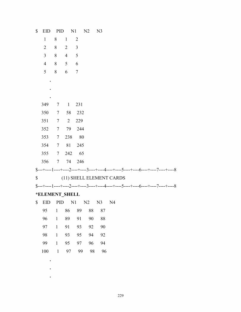
229
$ EID PID N1 N2 N3
1 8 1 2
2 8 2 3
3 8 4 5
4 8 5 6
5 8 6 7
.
.
.
349 7 1 231
350 7 58 232
351 7 2 229
352 7 79 244
353 7 238 80
354 7 81 245
355 7 242 65
356 7 74 246
$---+----1----+----2----+----3----+----4----+----5----+----6----+----7----+----8
$ (11) SHELL ELEMENT CARDS
$---+----1----+----2----+----3----+----4----+----5----+----6----+----7----+----8
*ELEMENT_SHELL
$ EID PID N1 N2 N3 N4
95 1 86 89 88 87
96 1 89 91 90 88
97 1 91 93 92 90
98 1 93 95 94 92
99 1 95 97 96 94
100 1 97 99 98 96
.
.
.
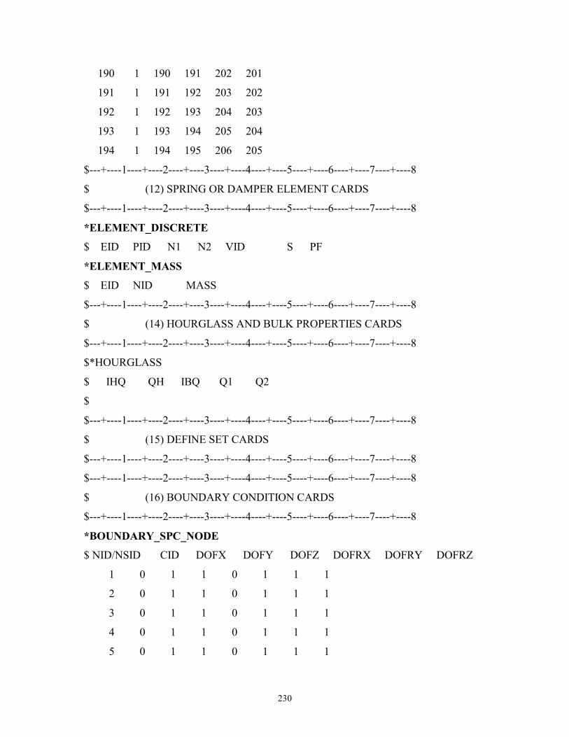
230
190 1 190 191 202 201
191 1 191 192 203 202
192 1 192 193 204 203
193 1 193 194 205 204
194 1 194 195 206 205
$---+----1----+----2----+----3----+----4----+----5----+----6----+----7----+----8
$ (12) SPRING OR DAMPER ELEMENT CARDS
$---+----1----+----2----+----3----+----4----+----5----+----6----+----7----+----8
*ELEMENT_DISCRETE
$ EID PID N1 N2 VID S PF
*ELEMENT_MASS
$ EID NID MASS
$---+----1----+----2----+----3----+----4----+----5----+----6----+----7----+----8
$ (14) HOURGLASS AND BULK PROPERTIES CARDS
$---+----1----+----2----+----3----+----4----+----5----+----6----+----7----+----8
$*HOURGLASS
$ IHQ QH IBQ Q1 Q2
$
$---+----1----+----2----+----3----+----4----+----5----+----6----+----7----+----8
$ (15) DEFINE SET CARDS
$---+----1----+----2----+----3----+----4----+----5----+----6----+----7----+----8
$---+----1----+----2----+----3----+----4----+----5----+----6----+----7----+----8
$ (16) BOUNDARY CONDITION CARDS
$---+----1----+----2----+----3----+----4----+----5----+----6----+----7----+----8
*BOUNDARY_SPC_NODE
$ NID/NSID CID DOFX DOFY DOFZ DOFRX DOFRY DOFRZ
1 0 1 1 0 1 1 1
2 0 1 1 0 1 1 1
3 0 1 1 0 1 1 1
4 0 1 1 0 1 1 1
5 0 1 1 0 1 1 1
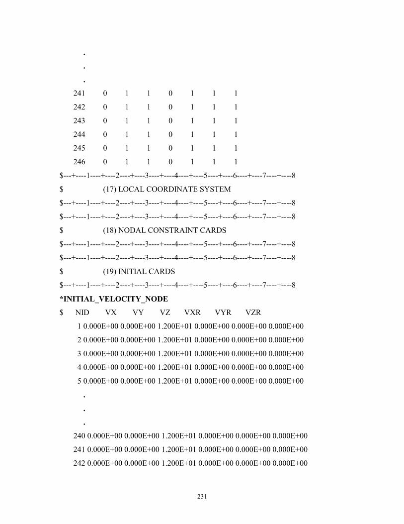
231
.
.
.
241 0 1 1 0 1 1 1
242 0 1 1 0 1 1 1
243 0 1 1 0 1 1 1
244 0 1 1 0 1 1 1
245 0 1 1 0 1 1 1
246 0 1 1 0 1 1 1
$---+----1----+----2----+----3----+----4----+----5----+----6----+----7----+----8
$ (17) LOCAL COORDINATE SYSTEM
$---+----1----+----2----+----3----+----4----+----5----+----6----+----7----+----8
$---+----1----+----2----+----3----+----4----+----5----+----6----+----7----+----8
$ (18) NODAL CONSTRAINT CARDS
$---+----1----+----2----+----3----+----4----+----5----+----6----+----7----+----8
$---+----1----+----2----+----3----+----4----+----5----+----6----+----7----+----8
$ (19) INITIAL CARDS
$---+----1----+----2----+----3----+----4----+----5----+----6----+----7----+----8
*INITIAL_VELOCITY_NODE
$ NID VX VY VZ VXR VYR VZR
1 0.000E+00 0.000E+00 1.200E+01 0.000E+00 0.000E+00 0.000E+00
2 0.000E+00 0.000E+00 1.200E+01 0.000E+00 0.000E+00 0.000E+00
3 0.000E+00 0.000E+00 1.200E+01 0.000E+00 0.000E+00 0.000E+00
4 0.000E+00 0.000E+00 1.200E+01 0.000E+00 0.000E+00 0.000E+00
5 0.000E+00 0.000E+00 1.200E+01 0.000E+00 0.000E+00 0.000E+00
.
.
.
240 0.000E+00 0.000E+00 1.200E+01 0.000E+00 0.000E+00 0.000E+00
241 0.000E+00 0.000E+00 1.200E+01 0.000E+00 0.000E+00 0.000E+00
242 0.000E+00 0.000E+00 1.200E+01 0.000E+00 0.000E+00 0.000E+00
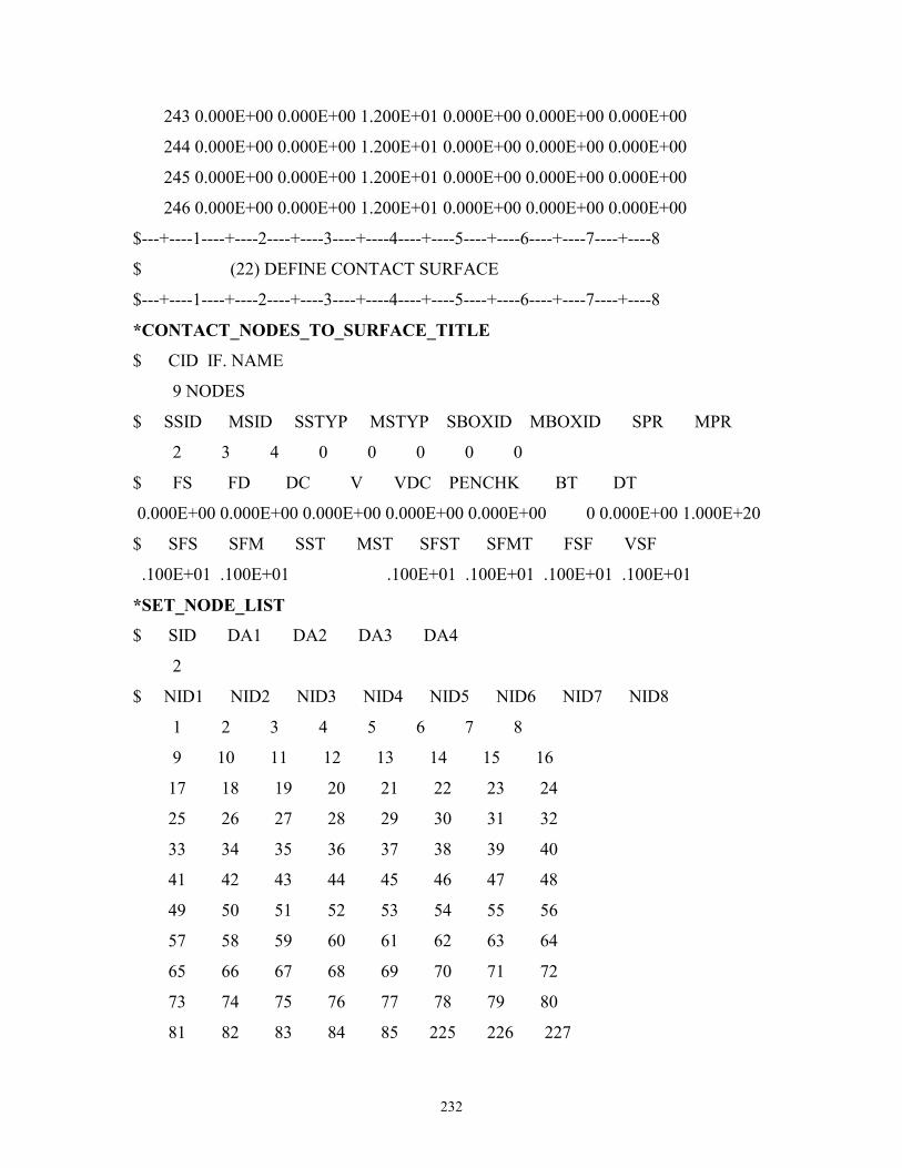
232
243 0.000E+00 0.000E+00 1.200E+01 0.000E+00 0.000E+00 0.000E+00
244 0.000E+00 0.000E+00 1.200E+01 0.000E+00 0.000E+00 0.000E+00
245 0.000E+00 0.000E+00 1.200E+01 0.000E+00 0.000E+00 0.000E+00
246 0.000E+00 0.000E+00 1.200E+01 0.000E+00 0.000E+00 0.000E+00
$---+----1----+----2----+----3----+----4----+----5----+----6----+----7----+----8
$ (22) DEFINE CONTACT SURFACE
$---+----1----+----2----+----3----+----4----+----5----+----6----+----7----+----8
*CONTACT_NODES_TO_SURFACE_TITLE
$ CID IF. NAME
9 NODES
$ SSID MSID SSTYP MSTYP SBOXID MBOXID SPR MPR
2 3 4 0 0 0 0 0
$ FS FD DC V VDC PENCHK BT DT
0.000E+00 0.000E+00 0.000E+00 0.000E+00 0.000E+00 0 0.000E+00 1.000E+20
$ SFS SFM SST MST SFST SFMT FSF VSF
.100E+01 .100E+01 .100E+01 .100E+01 .100E+01 .100E+01
*SET_NODE_LIST
$ SID DA1 DA2 DA3 DA4
2
$ NID1 NID2 NID3 NID4 NID5 NID6 NID7 NID8
1 2 3 4 5 6 7 8
9 10 11 12 13 14 15 16
17 18 19 20 21 22 23 24
25 26 27 28 29 30 31 32
33 34 35 36 37 38 39 40
41 42 43 44 45 46 47 48
49 50 51 52 53 54 55 56
57 58 59 60 61 62 63 64
65 66 67 68 69 70 71 72
73 74 75 76 77 78 79 80
81 82 83 84 85 225 226 227
233
228 229 230 231 232 233 234 235
236 237 238 239 240 241 242 243
244 245 246
*SET_SEGMENT
$ SID DA1 DA2 DA3 DA4
3
$ N1 N2 N3 N4 A1 A2 A3 A4
86 89 88 87
89 91 90 88
91 93 92 90
93 95 94 92
95 97 96 94
.
.
.
190 191 202 201
191 192 203 202
192 193 204 203
193 194 205 204
194 195 206 205
$---+----1----+----2----+----3----+----4----+----5----+----6----+----7----+----8
$ (23) DEFINE RIGID WALL
$---+----1----+----2----+----3----+----4----+----5----+----6----+----7----+----8
$ (24) NODAL RIGID BODY CARDS
$---+----1----+----2----+----3----+----4----+----5----+----6----+----7----+----8
$ (25) JOINT CARDS
$---+----1----+----2----+----3----+----4----+----5----+----6----+----7----+----8
$---+----1----+----2----+----3----+----4----+----5----+----6----+----7----+----8
$---+----1----+----2----+----3----+----4----+----5----+----6----+----7----+----8
*END

234
*LS-DYNA KEYWORDS are shown in bold-faced text.
The * preceding the keywords is a must and should not be ignored
The $ preceding a line means that that line is a dummy line and will not be executed
during the run.
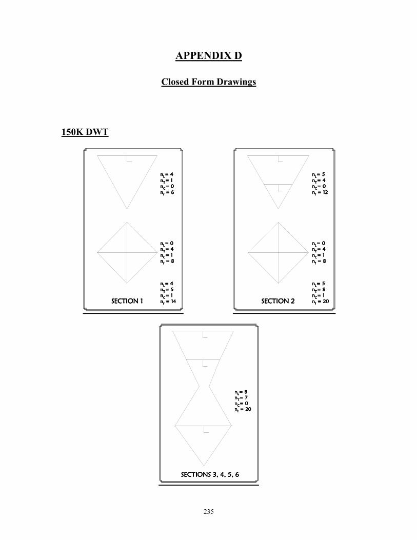
235
APPENDIX D
Closed Form Drawings
150K DWT
SECTION 1SECTION 1SECTION 1SECTION 1
nnnnLLLL= 4= 4= 4= 4nnnnTTTT= 1= 1= 1= 1nnnnCCCC= 0= 0= 0= 0nnnnffff = 6 = 6 = 6 = 6
nnnnLLLL= 0= 0= 0= 0nnnnTTTT= 4= 4= 4= 4nnnnCCCC= 1= 1= 1= 1nnnnffff = 8 = 8 = 8 = 8
nnnnLLLL= 4= 4= 4= 4nnnnTTTT= 5= 5= 5= 5nnnnCCCC= 1= 1= 1= 1nnnnffff = 14 = 14 = 14 = 14
SECTION 2SECTION 2SECTION 2SECTION 2
nnnnLLLL= 5= 5= 5= 5nnnnTTTT= 4= 4= 4= 4nnnnCCCC= 0= 0= 0= 0nnnnffff = 12 = 12 = 12 = 12
nnnnLLLL= 0= 0= 0= 0nnnnTTTT= 4= 4= 4= 4nnnnCCCC= 1= 1= 1= 1nnnnffff = 8 = 8 = 8 = 8
nnnnLLLL= 5= 5= 5= 5nnnnTTTT= 8= 8= 8= 8nnnnCCCC= 1= 1= 1= 1nnnnffff = 20 = 20 = 20 = 20
SECTIONS 3, 4, 5, 6SECTIONS 3, 4, 5, 6SECTIONS 3, 4, 5, 6SECTIONS 3, 4, 5, 6
nnnnLLLL= 8= 8= 8= 8nnnnTTTT= 7= 7= 7= 7nnnnCCCC= 0= 0= 0= 0nnnnffff = 20 = 20 = 20 = 20
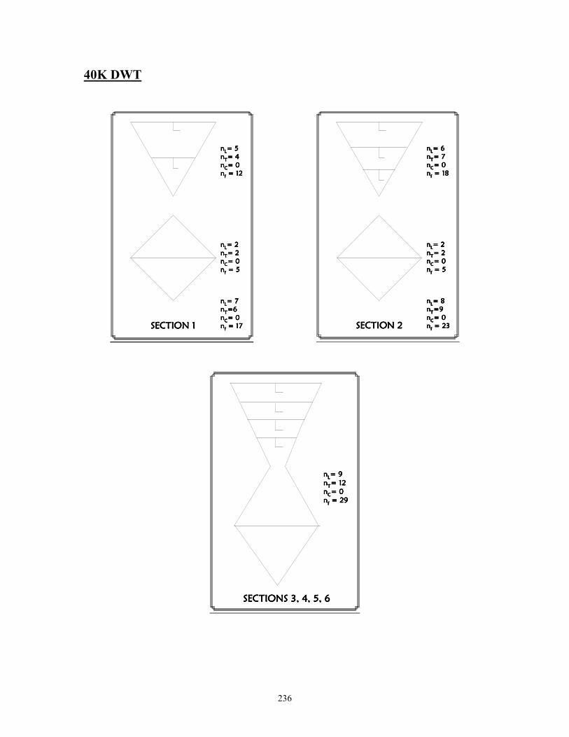
236
40K DWT
SECTION 1SECTION 1SECTION 1SECTION 1
nnnnLLLL= 5= 5= 5= 5nnnnTTTT= 4= 4= 4= 4nnnnCCCC= 0= 0= 0= 0nnnnffff = 12 = 12 = 12 = 12
nnnnLLLL= 2= 2= 2= 2nnnnTTTT= 2= 2= 2= 2nnnnCCCC= 0= 0= 0= 0nnnnffff = 5 = 5 = 5 = 5
nnnnLLLL= 7= 7= 7= 7nnnnTTTT=6=6=6=6nnnnCCCC= 0= 0= 0= 0nnnnffff = 17 = 17 = 17 = 17
SECTION 2SECTION 2SECTION 2SECTION 2
nnnnLLLL= 6= 6= 6= 6nnnnTTTT= 7= 7= 7= 7nnnnCCCC= 0= 0= 0= 0nnnnffff = 18 = 18 = 18 = 18
nnnnLLLL= 2= 2= 2= 2nnnnTTTT= 2= 2= 2= 2nnnnCCCC= 0= 0= 0= 0nnnnffff = 5 = 5 = 5 = 5
nnnnLLLL= 8= 8= 8= 8nnnnTTTT=9=9=9=9nnnnCCCC= 0= 0= 0= 0nnnnffff = 23 = 23 = 23 = 23
SECTIONS 3, 4, 5, 6SECTIONS 3, 4, 5, 6SECTIONS 3, 4, 5, 6SECTIONS 3, 4, 5, 6
nnnnLLLL= 9= 9= 9= 9nnnnTTTT= 12= 12= 12= 12nnnnCCCC= 0= 0= 0= 0nnnnffff = 29 = 29 = 29 = 29
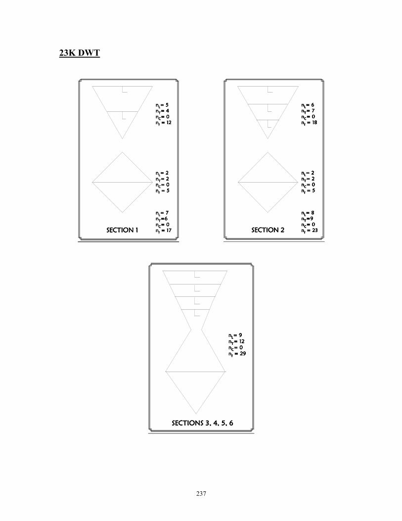
237
23K DWT
SECTION 1SECTION 1SECTION 1SECTION 1
nnnnLLLL= 5= 5= 5= 5nnnnTTTT= 4= 4= 4= 4nnnnCCCC= 0= 0= 0= 0nnnnffff = 12 = 12 = 12 = 12
nnnnLLLL= 2= 2= 2= 2nnnnTTTT= 2= 2= 2= 2nnnnCCCC= 0= 0= 0= 0nnnnffff = 5 = 5 = 5 = 5
nnnnLLLL= 7= 7= 7= 7nnnnTTTT=6=6=6=6nnnnCCCC= 0= 0= 0= 0nnnnffff = 17 = 17 = 17 = 17
SECTION 2SECTION 2SECTION 2SECTION 2
nnnnLLLL= 6= 6= 6= 6nnnnTTTT= 7= 7= 7= 7nnnnCCCC= 0= 0= 0= 0nnnnffff = 18 = 18 = 18 = 18
nnnnLLLL= 2= 2= 2= 2nnnnTTTT= 2= 2= 2= 2nnnnCCCC= 0= 0= 0= 0nnnnffff = 5 = 5 = 5 = 5
nnnnLLLL= 8= 8= 8= 8nnnnTTTT=9=9=9=9nnnnCCCC= 0= 0= 0= 0nnnnffff = 23 = 23 = 23 = 23
SECTIONS 3, 4, 5, 6SECTIONS 3, 4, 5, 6SECTIONS 3, 4, 5, 6SECTIONS 3, 4, 5, 6
nnnnLLLL= 9= 9= 9= 9nnnnTTTT= 12= 12= 12= 12nnnnCCCC= 0= 0= 0= 0nnnnffff = 29 = 29 = 29 = 29
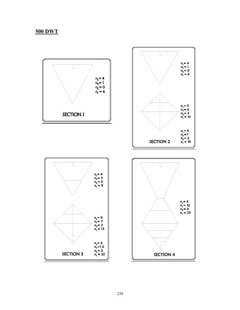
238
500 DWT
SECTION 1SECTION 1SECTION 1SECTION 1
nnnnLLLL= 4= 4= 4= 4nnnnTTTT= 1= 1= 1= 1nnnnCCCC= 0= 0= 0= 0nnnnffff = 6 = 6 = 6 = 6
SECTION 2SECTION 2SECTION 2SECTION 2
nnnnLLLL= 4= 4= 4= 4nnnnTTTT= 1= 1= 1= 1nnnnCCCC= 0= 0= 0= 0nnnnffff = 6 = 6 = 6 = 6
nnnnLLLL= 0= 0= 0= 0nnnnTTTT= 6= 6= 6= 6nnnnCCCC= 2= 2= 2= 2nnnnffff = 13 = 13 = 13 = 13
nnnnLLLL= 4= 4= 4= 4nnnnTTTT=7=7=7=7nnnnCCCC= 2= 2= 2= 2nnnnffff = 19 = 19 = 19 = 19
SECTION 3SECTION 3SECTION 3SECTION 3
nnnnLLLL= 4= 4= 4= 4nnnnTTTT= 3= 3= 3= 3nnnnCCCC= 0= 0= 0= 0nnnnffff = 9 = 9 = 9 = 9
nnnnLLLL= 0= 0= 0= 0nnnnTTTT= 7= 7= 7= 7nnnnCCCC= 2= 2= 2= 2nnnnffff = 13 = 13 = 13 = 13
nnnnLLLL= 4= 4= 4= 4nnnnTTTT=1 0=1 0=1 0=1 0nnnnCCCC= 2= 2= 2= 2nnnnffff = 22 = 22 = 22 = 22
SECTION 4SECTION 4SECTION 4SECTION 4
nnnnLLLL= 4= 4= 4= 4nnnnTTTT= 12= 12= 12= 12nnnnCCCC= 0= 0= 0= 0nnnnffff = 23 = 23 = 23 = 23
239
VITA
Suryanarayana Vakkalanka was born in Hyderabad, India on 24 June, 1977. He
did his schooling at Siva Sivani Public School, Hyderabad, India and his pre-university
schooling at Little Flower Junior College, Hyderabad, India.
He joined the Indian Institute of Technology, Madras, India in 1994 and graduated
with a Bachelor of Technology (B.Tech) in Naval Architecture in June 1998.
He then attended Virginia Polytechnic Institute and State University (Virginia
Tech), Blacksburg, USA for his graduate studies. He received his Master of Science
(M.S) in Ocean Engineering in March 2000. His areas of interest are ship collisions and
finite element analysis. Currently, he is working with Microstrategy Inc., Falls Church,
VA, USA.