Purdue UniversityPurdue e-PubsDepartment of Electrical and ComputerEngineering Technical Reports

Department of Electrical and ComputerEngineering

12-1-1989

Simple Model for Dissipation in QuantumTransportSupriyo DattaPurdue University

Follow this and additional works at: https://docs.lib.purdue.edu/ecetr

This document has been made available through Purdue e-Pubs, a service of the Purdue University Libraries. Please contact epubs@purdue.edu foradditional information.

Datta, Supriyo, "Simple Model for Dissipation in Quantum Transport" (1989). Department of Electrical and Computer EngineeringTechnical Reports. Paper 687.https://docs.lib.purdue.edu/ecetr/687

A Simple Model for Dissipation in Quantum Transport

Supriyo Datta

TR-EE 89-66 December 1989

School of Electrical EngineeringPurdue UniversityWest Lafayettev Indiana 47907

Supported by the National Science Foundation (Grant no. ECS-83-51-036) and the Semiconductor Research Corporation (Contract no. 88-SJ-0S9).

A SIMPLE MODEL FOR DISSIPATION

IN QUANTUM TRANSPORT

Supriyo Datta

School of Electrical Engineering Purdue University

West Lafayette, Indiana 47907

Technical Report: TR-EE 89-66 December 1989

LIMITED DISTRIBUTION NOTICE: The contents of this report will be submitted for publica­tion and will be copyrighted if accepted. The distribution of this technical report should be lim­ited to peer communications and specific requests.

Supported by the National Science Foundation (Grant no. ECS-83-51-036) and the Semiconduc­tor Research Corporation (Contract no. 88-SJ-089).

- 2 -

1. Introduction

Much of the current theoretical work on mesoscopic structures is based on the

Landauer-Biittiker formula which relates the currents Ii at the probes i to the electro­

chemical potentials μj at the probes j [1].

where

T i Pi - 2 T ij I1J j

Ti - X T i j= S T jij i

Tij(B) = Tji(-B)

( l . D

( 1.2)

(1.3)

B being the magnetic field. Eq. (1.1) has been justified from linear response theory [2]

and has been very successful in explaining many experimental observations [3]. How­

ever, there are a number of unresolved questions:

(I) How can we compute the transmission coefficients Tij in the presence of

phase-breaking scattering processes within die device starting from a micros­

copic model for the scatterers? Usually the coefficients Tij are computed

from the one-electron Schrodinger equation assuming that transport through

the device is phase-coherent.

(2) How can we describe harmonic generation [4] and large signal response [5]

which have been observed experimentally? Eq. (1.1) describes linear

response only.

(3) How can we compute the electron density in the device so that the band­

bending can be determined self-consistendy from the Poisson equation?

Space-charge effects are commonly neglected.

- 3 -

This paper represents an attempt to provide answers to these questions assuming a simple

model for the phase-breaking scattering processes [6].

The approach we adopt is closely related to the techniques [7-11] that have been

widely used to derive quantum kinetic equations describing the evolution of the non­

equilibrium Green function

G<(r1,r2;t1,t2) = |- ( V +(r2 ,t2)x|/(ri,ti)) (1.4)

where \|/(r, t) is the electron field operator. It is common to transform to center of mass

r = (I41 + r2)/2, t = ( t i+ t2)/2 (1,5a)

and relative coordinates, and then Fourier transform with respect to the relative coordi­

nate

i*i - r2 -4 k, tj - 12 -4 E (1.5b)

to obtain G^rjkjEjt). A number of authors have used the Wigner function fw(r;k;t)

which is obtained by integrating die Green function over energy [12,13]

fw( r ;k ; t ) ^ - i f - ^ % G <(r;k;E;t) = - iG <(r;k;t = t1 = t2) (1,6)J 2n n

The kinetic equation we derive is formulated in terms of the electron density per

unit energy n(r;E) which is obtained by integrating the Green function over k and t.

n(r;E) = - i J dt J G<(r;k;E;t) = - i J dt G ^ r= I4i = r2;E;t) (1.7)

The averaging over the time variable t= (tx -l-t2)/2 is made possible by our restriction to

steady-state, while the averaging over k is made possible by assuming a special form for

the phase-breaking scatterers. We assume that the scattering is caused by a distribution

of independent oscillators, each of which interacts with the electrons through a delta

potential. We also assume that the phase-breaking processes are weak and infrequent,

just as one does in deriving Fermi’s golden rule (however, the elastic scattering

- 4 -

processes are treated exactly). In the "golden rule" approximation, each scatterer acts

independently. Since we have assumed a delta interaction potential, an inelastic scatter­

ing event only involves the wavefunction at a particular point and is insensitive to spatial

correlations. This allows us to write a transport equation that only involves the diagonal

elements G<(r,r;E) of the Green functions. Spatial correlations of the field represented

by the off-diagonal elements G*1 Cr1, r2; E), T1 * r2 do not appear in this equation.

This simplification is important for two reasons. Firstly, the number of independent

variables is reduced from (rl5r2;E) (or equivalently, (r;k;E)> to (r;E) making it simpler

to obtain numerical solutions. Secondly, the diagonal elements are positive quantities

with simple physical interpretations such as the electron density per unit energy n(r;E).

This allows us to develop a simple physical picture for the transport process. We

emphasize that the use of r and E simultaneously does not violate the uncertainty princi­

ple. As shown in (1.5b) the energy spectrum is derived from the temporal correlations of

the wavefunction at a point r and bears no relationship to k which has to do with the spa­

tial correlations. We are not using conjugate variables like r and k or E and t simultane­

ously.

An obvious question to ask is whether this model is realistic. It closely approxi­

mates a laboratory sample with magnetic impurities or impurities having internal degrees

of freedom. For other types of phase-breaking scattering processes, the model may not

be accurate; however, it may still be possible to describe much of the essential physics of

dissipation in quantum transport. At the very least, we have a well-defined microscopic

model whose predictions can be worked out numerically for realistic structures and com­

pared with experiment. This should enable us to identify new phenomena arising from

spatially correlated inelastic scattering processes and many-body effects that are

neglected in our model.

- 5 -

In this paper we adopt a microscopic approach starting from a model Hamiltonian

for the inelastic scatterers; however, our model is closely related to the Landauer picture.

Since the inelastic scattering process is purely local, it can be viewed as an exit into a

reservoir followed by reinjection into the main structure [14, 15], From this point of view

it would seem that distributed inelastic scattering processes can be simulated by connect­

ing a continuous distribution of reservoirs throughout a structure. Indeed, when we sim­

plify our transport equation to linear response we obtain what looks like (1.1) generalized

to include a continuous distribution of probes. A direct generalization of (1.1), however,

would appear to be a phenomenological approach to simulating inelastic scattering. This

paper provides the rigorous justification for such an approach, by deriving the transport

equation directly from a model Hamiltonian making certain well-defined assumptions; it

also provides quantitative expressions for the transmission coefficients.

The outline of this paper is as follows. In Section 2 we describe the microscopic

model that we assume and derive the self-energy functions. In Section 3 we derive the

general kinetic equation which we believe can be used to describe large signal response.

In Section 4 we simplify the kinetic equation assuming local thermodynamic equili­

brium. We believe that this simplified equation can be used to describe linear and non­

linear response at low bias voltages. In Section 5 we specialize to linear response and

obtain an equation that looks like (1.1) generalized to a continuous distribution of probes.

We also show that this equation can be reduced to (1.1) and obtain an explicit expression

for Tij. Moreover, in a homogeneous medium with a slowly varying electrochemical

potential this equation reduces to the familiar diffusion equation. In this paper we have

defined the electrochemical potential p.(r) in terms of the diagonal element G<(r,r;E).

Since |i(r) is thus defined throughout the structure under conditions of local thermo­

dynamic equilibrium, an interesting question to ask is whether it can be measured by a

weakly coupled non-invasive probe. We also show in Section 5 that such a probe meas­

ures a weighted average of the potentials within a region of the order of a phase-breaking

- 6 -

length. The weighting function is characteristic of the probe geometry and construction.

Finally we conclude in Section 6 by summarizing the key results. In the main paper we

have tried to emphasize the physical interpretation of the results, relegating the

mathematical details to Appendices A through E.

2. Microscopic Model

We consider any arbitrary structure in which the propagation of electrons is

described by a one-electron effective mass Hamiltonian of the form

H0 = [p~ eyMriI l + eV(r) (2.1)2m

where m* is the effective mass. The scalar potential V(r) is the Hartree potential

obtained from a self-consistent solution of the Poisson equation. It includes band-

bending due to space charge and external bias, band discontinuities due to heterojunc­

tions, as well as all sources of elastic scattering such as impurities, defects and boun­

daries. This part of the Hamiltonian (H0) will be treated exactly.

The phase-breaking scattering is assumed to be due to a reservoir of independent

oscillators labeled by the index m,

H R - ^ lT C D ^ a m + h (2.2)m

where a^ and am are the creation and annihilation operators for oscillator m. We assume

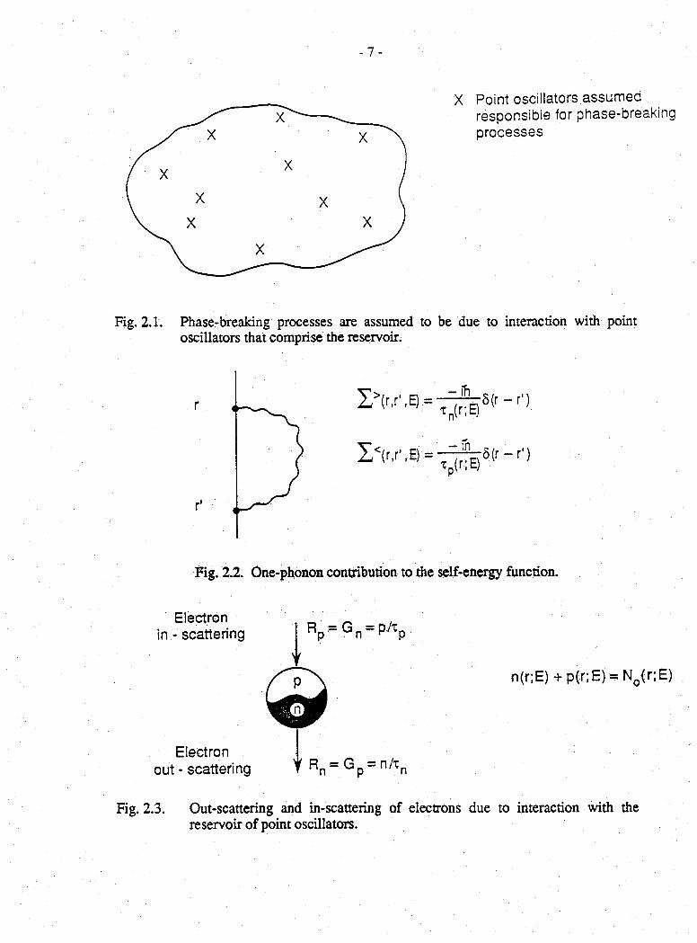
that each oscillator interacts with the electrons through a delta-potential (Fig. 2.1), so that

the interaction Hamiltonian H' can be written as

H' = X U 5 ( r - r m)(aJ1+ am) (2.3)m

Note that we have assumed the interaction strength U to be constant. There is no loss of

- 7 -

X Point oscillators assum ed responsible for phase-breaking processes

Fig. 2.1. Phase-breaking processes are assumed to be due to interaction with point oscillators that comprise the reservoir.

^ eI = f e S(r- r,)

^ <(r’r ' - E) = ^ f e 5 f r - r )

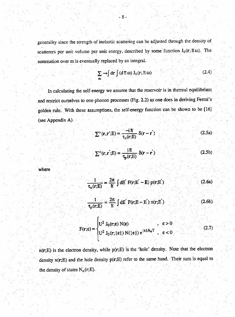
Fig. 2.2. One-phonon contribution to the self-energy function.

Electron in - scattering r P = g H = P7xP

V

Electronout - scattering T Rn = G p = n7tn

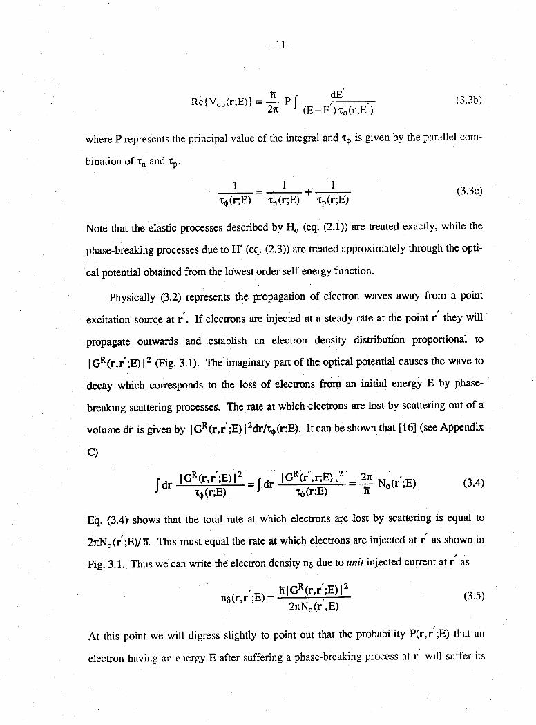
n(r;E) + p(r;E) = N0(r;E)

Fig. 2.3. Out-scattering and in-scattering of electrons due to interaction with the reservoir of point oscillators.

generality since the strength of inelastic scattering can be adjusted through the density of

scatterers per unit volume per unit energy, described by some function Jo(r; Hco). The

summation over m is eventually replaced by an integral.

X ^ J d r J (d IT co) J0 (r; IT co) (2.4)

In calculating the self-energy we assume that the reservoir is in thermal equilibrium

and restrict ourselves to one-phonon processes (Fig. 2.2) as one does in deriving Fermi’s

golden rule. With these assumptions, the self-energy function can be shown to be [16]

(see Appendix A)

X>(r,r';E):

X<(r,r';E) =

—ilT s / . ' v> Pv 8 r - r ) xn(r;E)

(2.5a)

iE 5, s— —— 5(r - r ) Xp(r;E)

(2.5b)

where

%(r;E) HJ dE F(r;E - E) p(r;E )

M I d E F ( r ;E -E ) n(r;E)xp(r;E) E

F(r;e);U2 J0(r;e)N(e) , e > 0

U2 J0( r ; |e |) N ( |e |) e |E|/kBT , e < 0

(2.6a)

(2.6b)

(2.7)

n(r;E) is the electron density, while p(r;E) is the ‘hole’ density. Note that the electron

density n(r;E) and the hole density p(r;E) refer to the same band. Their sum is equal to

the density of states N0(r;E).

n(r;E) + p(r;E) = N0(r;E) = £ |<|>M(r) | 2 8(E -E m) (2 .8)

Here (J)M(r) are the eigenfunctions of H0 (eq. (2.1)) with eigenvalues Em- We have

neglected any level broadening due to interaction with the reservoir. N(ITco) is the aver­

age number of ‘phonons’ in an oscillator of frequency CO and is given by the Bose-

Einsteinfactor

N<R“ >= T n s s r - T <-9JC — I

It is easy to see why the self-energy functions in our model are delta functions in space.

Since we consider only one phonon processes, the electron interacts with the same oscil­

lator at r and r (Fig. 2.2). But the interaction potential has been assumed to be a delta

function at the location rm of the oscillator. Hencer and r must both coincide with rm.

The similarity of (2.6a, b) to Fermi’s golden rule will be noted. However, unlike

the usual golden rule we are not using energy eigenstates. We are using the position

representation and a simple golden rule-like result is not valid in general. Itis made pos­

sible by our assumption of independent point oscillators that only see the electron

wavefunction at one point. In this model, the phase-breaking scattering process is a

purely local affair that shuffles the energy E of the electrons at a fixed point r. The rate

Rn at which electrons are scattered out of energy E at the point r (or the rate Gp at which

holes are scattered in) is proportional to the imaginary part of 2^(r,r;E) (eq. (2.5a)).

R„<r;R) = ^ § r = OpfnF-) (2.10a)

Similarly the rate Rp at which holes are scattered out is equal to the rate Gn at which

electrons are scattered in and is proportional to the imaginary part of E<(r,r;E) (eq.

-TO-

Rp(r;E) = - ^ § - = Gn(r;E) (2.10b)

The out-scattering and in-scattering of electrons is shown schematically in Fig. 2.3.

It will be noted that if the energy distribution of electrons is given by the Fermi-

Dirac factor with some local electrochemical potential |X(r)

n(r;E)N0(r;E)

(2.11)

then the out-scattering and in-scattering rates exactly balance each other.

n(r;E) _ p(r;E) tn(r;E) xp(r;E)

(2.12)

This is shown in Section 4.

3. KineticEquation

Starting from the Dyson equation in the Keldysh formulation and using the

appropriate self-energy functions (eqs. (2.5a, b)) it can be shown that [6,16] (see Appen­

dix B) ;

- I [dr- l ° Rfr-f';E)|2 2n J Tp (r ;E)

(3.1)

where the retarded Green function GR(r,r';E) is obtained from the Schrodinger equation

modified to include an ‘optical potential’ Vop. Because the self-energy is a delta function

in space, Vop (r;E) is a simple local potential.

|e - Ho(r) - Vop(r;E)j GR(r,r';E) = 5(r - r ') (3.2)

Im{Vop(r;E)} = IT2t0(r;E)

(3.3a)

- 11 -

(3.3b)

where P represents the principal value of the integral and is given by the parallel com­

bination of xn and Xp.

Note that the elastic processes described by H0 (eq. (2.1» are treated exactly, while the

phase-breaking processes due to H' (eq. (2.3)) are treated approximately through the opti­

cal potential obtained from the lowest order self-energy function.

Physically (3.2) represents the propagation of electron waves away from a point

propagate outwards and establish an electron density distribution proportional to

|GR(r,r';E) I2 (Fig. 3.1). The imaginary part of the optical potential causes the wave to

decay which corresponds to the loss of electrons from an initial energy E by phase-

breaking scattering processes. The rate at which electrons are lost by scattering out of a

volume dr is given by | GR(r,r';E) 12dr/x<!)(r;E). It can be shown that [16] (see Appendix

Eq. (3.4) shows that the total rate at which electrons are lost by scattering is equal to

2jtN0(r;E)/lT. This must equal the rate at which electrons are injected at r as shown in

Fig. 3.1. Thus we can write the electron density ns due to unit injected current at r as

(3.3c)

excitation source at r . If electrons are injected at a steady rate at the point r they will

C)

(3.4)

n5(r,r ;E) =fi|GR(r ,r ;E ) |2

27tN0(r',E)(3.5)

At this point we will digress slightly to point out that the probability P(r,r ;E) that an/

electron having an energy E after suffering a phase-breaking process at r will suffer its

- 12 -

G

l f No'r'-

I

Position

Fig. 3.1. Propagation of electron waves away from a point excitation. The argument E has been suppressed for simplicity.

-13

next phase-breaking scattering at r is given by

'P(r,r ;E)' = n5(r,r^)/T^'(r;E)

_ B |G R(r,r ;E )|2 6)2w N0(r;E)x^(r;E)

This relation is important because the probability function P(r,r ;E) can also be com­

puted semiclassically using a Monte Carlo approach and a comparison of the semiclassi-

cal result with the quantum mechanical result could be illuminating. In fact we believe

that by replacing { Gr | 2 in (3.1) with the appropriate semiclassically computed quantity,

it is possible to use the equations derived in this paper to describe semiclassical transport

as well. ■

We now turn to a physical interpretation of the kinetic equation, (3.1) which can be

rewritten as

f 4 ' / ' ^ N0(r';E) . _n(r;E) = j dr n§(r,r ;E) * , (3,7)

%(r ;E) v.;

The net electron density n(r;E) can be viewed as a superposition of the electron densities

due to point sources at different points r' (Fig. 3.2). Since n8(r,r';E) is the electron den­

sity due to unit injected current at r , (3.7) is readily understood if the rate Gn of in­

scattering of electrons is identified with

Gn(r;E) = N0(r;E)/Tp(r;E) (3.8)

Note that this is somewhat larger than the in-scattering rate Gn discussed in Section 2

[eq. (2.10b)]

Gn(r:F.)=Gn(r;n) + ^ ^ - (3.9a)

This excess in-scattering is exactly balanced by an excess in the Out-scattering. Eq. (3.2)

describes the propagation of electrons that are lost by scattering at the rate

Fig. 3.2. The electron density n(r;E) is obtained by superposing the individual densities due to a continuous distribution of point sources.

IZ D P

I W l n

An

Fig. 3.3. In the contacts the external current I(r;E) causes a change in the electron density by An(r;E).

- 15 -

Rn = ri(r;E)/T<j)(r;E) which is larger than the outscattering rate Rn discussed in Section 2

[eq. (2.10a)].

Rn(r;E) = Rn( r ; E ) + - ^ a . (3.9b)

The excess scattering rate (Rn - R n) or (Gn-G n) is negligible for a dilute electron gas

with n(r;E) < < p(r;E) - N0(r;E). But for a degenerate electron gas, n/tp represents the

part of the in-scattering that is inhibited by the exclusion principle. The physical

interpretation of (3.1) presented above suggests that phase-coherence is destroyed despite

the Pauli-blocking.

External Current: So far we have not considered any external sources of current at

the contacts. We assume that the external current causes an excess An(r;E) in the elec­

tron density to build up. To account for this build-up, the kinetic equation, (3.1), is

modified to read

n(r;E) J5_2k

r dr' |GR(r,r ;E)l2 J tp(r ;E)

+ An(r;E) (3.10)

The excess electron density leads to an excess out-scattering rate ARn=AnZr^ which is

balanced by the current I(r;E) from the external leads. Hence,

I(r;E) = eAn(r;E)/T0(r;E) (3.11)

Using (3.11) we can rewrite eq. (3.10) as

I(r;E)en(r;E) _ efi |G R(r ,r ;E ) |2 ^(r;E ) 2k J x6(r;E) xp(r';E)

(3.12)

Using eq. (2.6b) to replace xp(r ;E) in terms of the electron density we obtain an integral

equation for n(r;E) as follows.

- 16 -

I(r;E) = - T - ^ r — e J dr J Cffi K(r,r ,E,E ) n(r ;E ) (3.13)

where

K(r,r';E ,E) = |GR(r,r';E) | 2 F(r';E -E)/^(r;E ) (3.14)

The above procedure for including the external current source assumes that the

current is injected incoherently. Eq. (3.13) can be solved numerically for practical struc­

tures by dividing it up into ‘contact’ regions which are assumed to be in local thermo­

dynamic equilibrium with a given electrochemical potential and ‘device’ regions where

the electron density is free to assume any form (Fig. 3.4). The electron density n(r;E) is

thus known in the contacts but unknown in the device, while the external current I(r;E) is

unknown in the contacts but known (to be zero) in the device.

A more rigorous approach for including the external current (that we will not pursue

further in this paper) is to solve (3,1) with the appropriate boundary conditions for n(r;E)

and then to evaluate the full Green function G<(r,r ;E) using the relation [6, 16] (see

Appendix B, eq. (B.15))

-IC cO*, r;E ) = K jd r1GR(r>r 1;E)GA(ri,r;E )

Tp(ri;E)(3.15)

We can then transform variables as indicated in (1.5a,b) to obtain G<(r;k;E) from which

the current density J(r;E) can be computed [10]. The external current I(r;E) can then be

obtained from the divergence of J.

4. Local Thermodynamic Equilibrium

We will now specialize to biasing conditions that are small enough that local ther­

modynamic equilibrium is maintained everywhere. The energy distribution of electrons

everywhere can then be written in the form shown in (2.11) which we restate here for

convenience.

- 17 -

contact

device

Fig. 3.4. The contact regions are each assumed to be in local thermodynamic equilibrium with a given electrochemical potential. The electron density n(r;E) is free to assume any form in the rest of the structure, labeled as ‘device’.

- 18 -

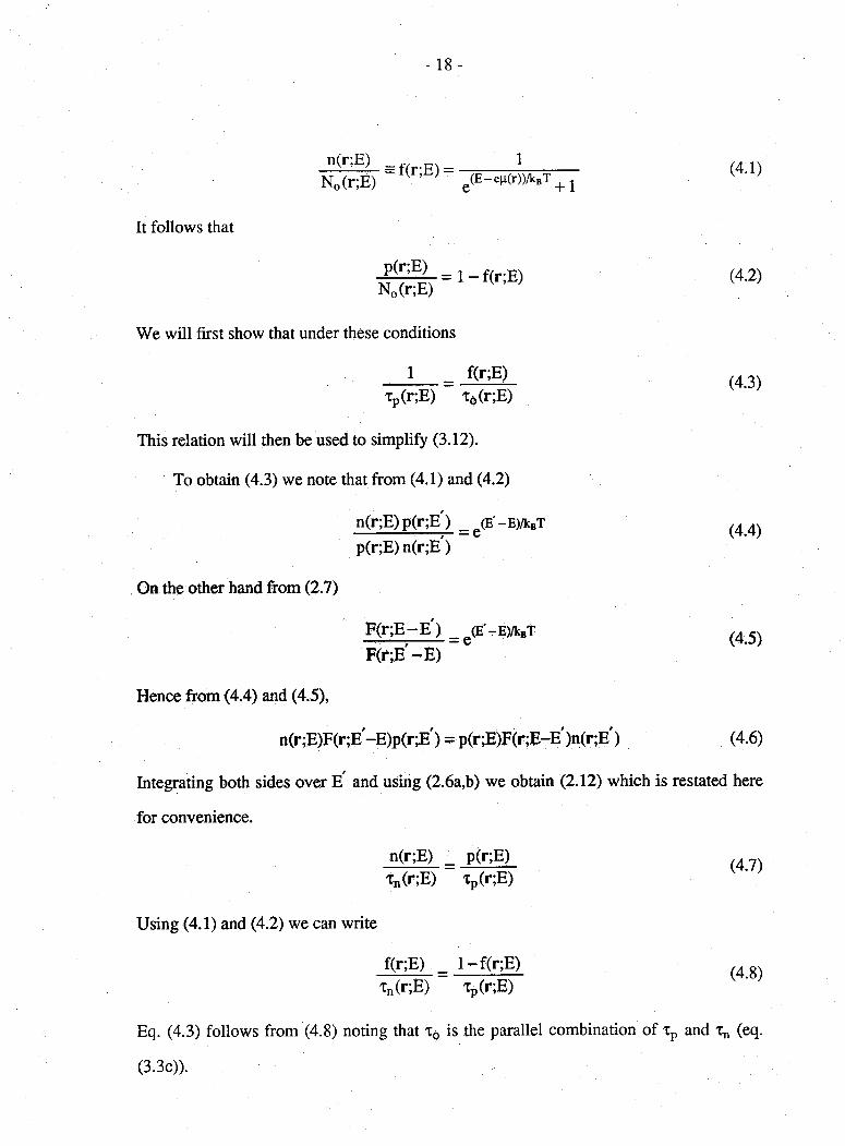
n(r;E)N0(r;E)

f(r;E): g(E-e|i(r))/kBT + j

It follows that

P(r;E)N0(r;E)

I - f(r;E)

We will first show that under these conditions

I f(r;E)Xp(r;E) X1J, (r;E)

This relation will then be used to simplify (3.12).

To obtain (4.3) we note that from (4.1) and (4.2)

n(r;E)p(r;E) _ (E'-E)/kBT■ C

On the other hand from (2.7)

p(r;E) n(r;E)

F (r ;E -E ) _ je '-Eyk8T■CF(r;E — E)

Hence from (4.4) and (4.5),

n(r;E)F(r;E -E)p(r;E ) = p(r;E)F(r;E-E )n(r;E )

(4,1)

(4.2)

(4.3)

(4.4)

(4.5)

(4.6)

Integrating both sides over E and using (2.6a,b) we obtain (2.12) which is restated here

for convenience.

n(r;E) _ p(r;E) xn(r;E) xp(r;E)

Using (4.1) and (4.2) we can write

f(r;E) _ l~f(r;E) xn(r;E) xp(r;E)

Eq. (4.3) follows from (4.8) noting that X(j, is the parallel combination of Xp and Xn (eq.

(3.3c)).

-1 9 -

Using (4.3) we can rewrite (3.12) as • ,V- v

I(r;E) = | - T (r;E )f(r;E )-Jd r T(r,r ;E:) f(r ;E)j (4.9)

where ‘ ■ ■ ' ...:: V V :, ■'

W ; K ) = n2 |GR<r.r-;F,|:T*(r;E)x*(r ;E)

(4V1O)

T(r;E) = hN0(r;E)/t<1)(r;E) (4.11)

It can be shown that the quantities T(r,r';E) and T(r;E) obey relations very similar to

(1.2) and (1.3) [16] (see Appendix C).

T(r;E) = J dr T(r,r';E) = J dr T(r',r;E) (4.12)

T(r,r ;E) Ib = T(r,r;E) |_B (4.13)

Note, however, that while (1.1) describes linear response only, (4.9) is capable of

describing non-linear response as well. In (1.1) the coefficients Ty are evaluated at

equilibrium. But in (4.9) the coefficients T(r,r';E) are computed in the presence o f an

applied bias. Consequently T(r,r';E) can be different for positive and negative bias for

asymmetric devices and the current I for a positive bias V may have a very different

magnitude compared to that for a negative bias leading to the generation of even harmon­

ics. By contrast in the Landauer-Biittiker formula the Ty are equilibrium quantities

independent of bias. Consequently the current response to an applied bias is precisely

linear. In the next section we will specialize (4.9) to linear response.

- 2 0 -

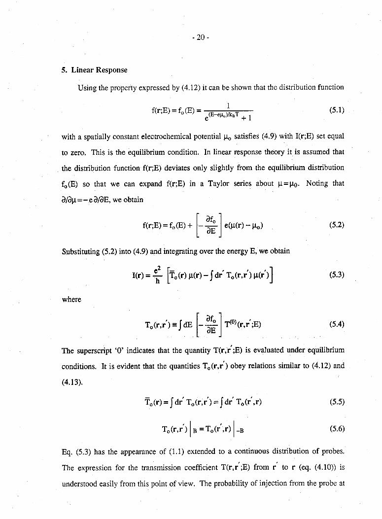
5. LinearResponse

Using the property expressed by (4.12) it can be shown that the distribution function

If(r;E) = f0(E): e (E-en0)/kBT + j (5.1)

with a spatially constant electrochemical potential (I0 satisfies (4.9) with I(r;E) set equal

to zero. This is the equilibrium condition. In linear response theory it is assumed that

the distribution function f(r;E) deviates only slightly from the equilibrium distribution

f0(E) so that we can expand f(r;E) in a Taylor series about |i=(io. Noting that

8/9(i=- e9/9E, we obtain

f(r;E) = f0(E) + e (it( r ) -^ 0) (5.2)

Substituting (5.2) into (4.9) and integrating over the energy E, we obtain

„2Kr) = Y [To(r ) ^ r> - J dr'T 0( r ,r ) |x ( r )] (5.3)

where

T0(r,r') = JdE9fo_9E

T ^ ( r ,r ;E) (5.4)

The superscript ‘0’ indicates that the quantity T(r,r ;E) is evaluated under equilibrium

conditions. It is evident that the quantities T0(r ,r ) obey relations similar to (4.12) and

(4.13).

T0(r) = J d r 'T 0(r,r') = J d r 'T 0(r',r) (5.5)

T0( r , r ) B =T 0(r ,r) -B (5.6)

Eq. (5.3) has the appearance of (1.1) extended to a continuous distribution of probes.

The expression for the transmission coefficient T(r,r ;E) from r to r (eq. (4.10)) is

understood easily from this point of view. The probability of injection from the probe at

-21 -

r is proportional to l/T<t>(r;E), that of propagation from r to r is proportional to

|GR(r ,r ;E ) |2 and that of ejection into the probe at r is proportional l/x^ (r;E). In fact

the same expression is obtained if we start from the Kubo formula for the non-local con­

ductivity tensor <r(r,r ;E) and use the Fisher-Lee formula [17] to obtain T (r,r ;E) [16]

(see Appendix D).

Landauer-Buttiker Formula

We will now reduce (5.3) to the same form as (LI) and obtain explicit expressions

for the transmission coefficients. We assume that within the structure there are ‘contact’

regions where the electrochemical potential has a constant value; the rest of the structure

is labeled the ‘device’ (Fig. 3.4). integrating (5.3) over all r included in contact i, we

obtain the total current Ii coming into contact i.

where

T0<i) m --X-T0(U)'Mj- j

I dr T0(i,r) n(r) r e device

Tjj = T0(Lj) = J dr J dr T0( r , r )rei, r ej

(5.7)

(5.8)

T0(i) = J d rT 0(r)rei

(5.9)

T0(U ) = J dr T0 (r\r) (5.10)re i

When we neglect phase-breaking processes within the device the last term in (5.7) is zero

(see eq. (4.10)) so that (5.7) reduces to the same form as (1.1). We will show below that

in general we can eliminate |0.(r) from (5.7) to write it in the same form as (1.1).

where

- 2 2 -

T 0 (i) Md ~ £ T ij M-j j

(5.11)

Tij = T0(IJ)+ T ^ + T f f + ••• (5.12)

^ - T 0(Ij r i )To(F1J) (5.13a)To(ri)

T1 € device

T f = I J T„(i.r,) T0( r , , r 2) T0Ir2J) (5.13b)T0Ir2) T0Ir2)

ri,r2€ device

and so on. This result may be viewed as a generalization of the result obtained by

Biittiker for a single floating probe [15]. The successive terms in (5.12) are shown

schematically in Fig. 5.1. The first term T0(iJ) is the probability of coherent transmis­

sion from contact ‘j ’ to contact T without suffering any phase-breaking scattering within

the device. The next term T ^ is the probability of transmission with one phase breaking

scattering event at some point T1 within the device; T[p is the probability of transmission

with two scattering events at T1 and within the device; and so on. It can be shown that

the coefficients Tij and T0(i) indeed satisfy the relations (1.2) and (1.3).

To obtain (5.11) from (5.7) we note that within the device, the current l(r)= 0 so

that ,

0 = fo(r) p(r) - X T0 ( r j) pj - Jd r' T0(r ,r )J if r ) , r e device (5.14)j r e device

or equivalently

contact

device

Fig. 5.1. Interpretation of successive terms in (5.12).

- 24 -

| i ( r ) = £ Jtj + J dr T°(r,r-- Ji(r') (5.15)j T0(r ) r’s device T0(r)

Eq. (5.15) can be solved to obtain the electrochemical potential |i(r) everywhere in the

device in terms of the potentials Jij in the contacts. The solution can be written in the

from of an iterative series as follows.

ji(r) = ji(1)(r) + Ji(2)(r) + • • • (5.16)

where/i\ _ To(r,j)

M-1 (r) = X - tij (5.17a)j T„(r)

p'”)(r)= Jd r1 Tl <r-ri) P1- 1Hr,) (5.17b). ; Fxedevice T0 (r) .

etc. Substituting ji(r) from (5.16) and (5.17a,b) into (5.7) we obtain (5.11).

Diffusion Equation

We would also like to point out that in a homogeneous medium we can reduce the

linear response equation (5.3) to the familiar diffusion equation, if |i(r) is assumed to

vary slowly. The integral operator on the right hand side of (5.3) then reduces to the

Laplacian operator as shown in Appendix E.

V - J = oV 2 ji(r) (5.18)

where o = |^ J d p p ; T ( p ) (5.19)

We have written p for r - r , noting that in a homogeneous medium T(r,r ) depends only

on the difference coordinate r - r ' . Here J(r) is the Cunrent density in the structure,

whose divergence equals the external probe current I(r).

- 2 5 -

Whatpotential does a ‘non-invasive’ probe measure?

In this paper we have defined the electrochemical potential p(r) rigorously in terms

of the electron density per unit energy n(r;E), assuming local thermodynamic equili­

brium (eq. (2.11)). An interesting question is whether this local electrochemical potential

p(r) can be measured using a weakly coupled probe [18]. We assume that the probe is

coupled weakly enough that it does not perturb the solution to (5.3) within the device

appreciably (Fig. 5.2); that is, the local electrochemical potential p(r) is assumed to stay

the same with and without the probe. The potential Pprobe to which the probe floats is

obtained from (5.3) by integrating over all r e probe and setting the current equal to zero.

O = Pprobe Jd r T0(r) - J dr J d r T0( r ,r ) p(r )r € probe r e probe

(5.20)

Hence, Hprobe = J dr' P(r')p(r') (5.21)

where P(r ) = Jd r T0( r , r )/ Jd r T0(r)re probe re probe

(5 .2 2 )

Note that (5 .2 1 ) can be viewed as an extension of Biittiker’s result (eq. ( I ) of [1 8 ]) to a

continuous distribution of reservoirs. Eq. (5 .2 1 ) shows that the potential Pprobe measured

by the probe is a weighted average of the potentials p ( r ) in different parts of the struc­

ture. Since T0(r,r') is proportional to I Gr(r , r ) | 2 which decays within a phase-breaking

length L(J), IiprObe is affected only by the potentials within a distance Llj,. If the potential

varies slowly within this distance then there is no ambiguity in the measured potential

Pprobe. But if the potential varies significantly within a phase-breaking length then the

potential PprObe that a probe measures depends on the probe function P(r). The probe

function P(r) represents the fraction of carriers entering the probe that suffered their last

phase-breaking scattering at r. Clearly this function depends on the probe-geometry and

- 26 -

PROBE

DEVICE

Hg. 5.2. A weakly coupled probe connected to a device floats to a potential MprObe that is a weighted average of the potential M(r) existing within a phase­breaking length Lb.

- 2 7 -

construction.

6. SUMMARY

Starting from a model Hamiltonian we have derived a simple transport equation that

can be solved (self-consistently with the Poisson equation) to obtain the electron density

per unit energy (r;E) in an arbitrary structure.

I(r;E) = en^ - e J dr J dE K(r,r';E,E ) n(r';E) (6.1)

In our simple model transport can be viewed as a diffusion process in (r;E). Each

phase-breaking scattering event causes a change in the energy of the electron at a fixed

point in space. Between two such phase-breaking processes the electron propagates in

space coherently with a fixed energy. The kernel K(r,r ;E ,E ) represents the transfer

function’ between two phase-breaking processes, the first at (r ;E ) and the next at (r;E).

We then assume local thermodynamic equilibrium to simplify (6.1)

I(TjE)= I* [f (r;E) f(r;E) - J dr' T (r,r ;E) f(r ;E)J (6.2)

Eq. (6.2) can be solved for the distribution function f(r;E)sn(r,E)/N0(r;E), N0(r;E)

being the density of states. Though we have assumed local equilibrium, (6.2) is still a

non-linear transport equation. Note that the coefficients T(r,r ;E) are not equilibrium

quantities, but are evaluated under the appropriate biasing conditions.

Next we specialize (6.2) to linear response and obtain an equation that has the

appearance of (1.1) extended to include a continuous distribution of probes.

Kr) = Y [T0(r) ii(r) - J dr' T0(r,r') li(r')J (6-3)

Wethen show that (6.3) can be reduced to (1.1) and obtain an explicit series solution for

the coefficients Tij appearing in (1.1). Also it can be shown that in a homogeneous

- 2 8 -

medium with a slowly varying electrochemical potential, (6.3) reduces to the diffusion

equation

V • J(r) = G V2 |i(r) (6.4)

The simplicity of our model leads to a clear physical picture of the transport pro­

cess. The transport equation is simple enough that numerical solutions (self-consistently

with the Poisson equation) seem feasible for practical structures. By Comparing the pred­

ictions of our model with experiment it should be possible to establish the limitations of

our model and identify new phenomena.

ACKNOWLEDGEMENTS

I would like to acknowledge Michael J. McLennan for many helpful discussions. I

also thank Markus Biittiker fora preprint of his work (Ref. 18). This work was supported

by the National Science Foundation under Grant No. ECS-8351036 and by the Semicon­

ductor Research Corporation under Contract No. 88-SJ-089.

-29

REFERENCES

1. Biittiker, M., 1986, Phys. Rev. Lett, 57,1761.

2. Stone, A. D., and Szafer, A., 1988, IBM J. Res. Dev. 32 384; Baranger, H.U., and

Stone, A.D., preprint.

3. See for example, Biittiker, M., 1988, IBM J. Res. Dev. 32, 317; Baranger, H.U.,

and Stone, A.D., 1989, Phys. Rev. Lett. 63 414; Szafer, A., and Stone, A.D., 1989,

Phys. Rev. Lett. 62 300.

4. deVegvar, P.G.N., Timp, G., Mankiewich, P. M., Cunningham, XE., Behringer, R.,

and Howard, R.E., 1988, Phys. Rev. B 38 4326.

5. A common example that has been studied widely is the resonant tunneling diode;

see, for example, Refs. 12,13.

6. Datta, S., 1989, Phys. Rev. B 40 5830.

7. Kadanoff, L.P., and Baym, G., 1962, Quantum Statistical Mechanics, (W.A. Ben­

jamin, Inc., New York).

8. Keldysh, L.V., 1965, Soviet Physics JETP 20 1018.

9. Langreth, D.C., 1976, Linear and Nonlinear Etectron Transport in Solids, ed.

Devreese, J.T., and Van Doren, E., (Plenum, New York).

10. Mahan, G D , 1987, Phys. Rep. 145 251.

11. Jauho, A.P., and Ziep, O., 1989, Physica Scripta T25 329; Jauho, A.P., 1989, Solid

State Electronics (to appear).

12. Frensley, W.R., 1987, Phys. Rev. B 36 1570.

13. Kluksdahl, N.C., Kriman, A.M., Ferry, D.K., Ringhofer, C., 1989, Phys. Rev. B 39

. 7720.

14 Engquist, H.L., and Anderson, P.W., 1981, Phys. Rev. B 24 1151.

- 30 -

15. Biittiker, M., 1988, IBM J. Res. Dev. 32 63.

16. Datta, S., et. al., 1989, Purdue University Technical Report, TR-EE 89-59

(Chapter 4).

17. Fisher, D.S., and Lee, P.A., 1981, R/rys. Rev. B 23 6851.

18. Biittiker, M., 1989, Phys. Rev. B. 40 3409.

19. Kubo, R., 1968, Rep. Progr. Phys. 29,255.

20. Doniach, S., and Sondheimer, E.H., 1974, Green’s Functionsfor Solid State Physi­

cists (Benjamin-Cummins).

-31 -

Appendix A: Derivation of Self-energy Functions

Our main objective in this Appendix is to derive (2.5a, b) and (2.6a, b). We will

also derive the retarded and advanced self-energy functions. We start from the relations

[10]

L>(X1,X2) = G>(X1,X2)D >(X1,X2) (A la)

X<(X1,X2) = G<(X1,X2)D <(X1,X2) (A. lb)

Here X stands for (r,t). The electron Green functions G>, G< are defined by

G>(X1,X2) = (V(X1) ^ t(X 2)) (A.2a)

G ^X 1 ,X2)= j (Vt (X2) V(X1)) (A.2b)

The functions D>, D4i are given by

D> (X15X2) = (H^rl5I1) H'(r2, t2» (A.3a)

D<(X1,X2) = <H'(r2,12W r l5I1)) (A.3b)

Using (2.3) for H' we obtain

D>(X,,X2) = U2 X Sfr1 - r m) 8(r2—rn) ( (a j^ ti)+ am(ti))(a |(t2) + an(t2)) >(A.4)m,n

We assume that the reservoir of oscillators is in a state of thermodynamic equilibrium, so

that

(Hja(I i)M t2)) = Srtm N(Ko)m) eioUtl~t2) (A.5a)

(am(ti) aj(t2)) = Smn (N(Ko)m) + I )e_i^ (tl_t2) (A.5b)

(am(ti) an(t2)) = 0 (A.5c)

( am(ti) a£(t2) ) = 0 (A.5d)

- 32 -

where N(E com) is the average number of "phonons" in a oscillator of frequency COm and is

given by the Bose-Einstein factor

NO1") = Eto/keT , (A6)6 I

Using (A.5a-d) we obtain from eq. (A.4),

D>(X1,X2) = U2 5(r i - r 2) E 5(r i - r m) [N(Ecom) eia (tl _t2)

+ (N(Ecom) + I )e i(0m(tl t2)] (A.7)

Replacing the sum over m by an integral (eq. (2.4)) and Fourier transforming

tj - t 2 —» ewe have,

D>(r! ,r2 ; e> = 2jcE U2 J0( r i ; I e I) 6(ri - r 2)

I n (IEI) , B<0N(e) + 1 , e > 0

Similarly it can be shown that

D<(ri,r2;e) = 2tcEU2 J0( r i ; |e |) SCri^r2)

J N(IeI) + 1 , e <0I N(e) , e > 0

(A. 8b)

To calculate the self-energy functions we Fourier transform (A. la,b)

5 ? (rj,r2 ;E) = f G>(ri ,T2 IE O D ^rl lF2 ;E-E0 (A.9a)J 2nn

Zc( W fE) = G ^ r ,,^ ; E') D-=Cr1,F2 IE-E1) (A.9b)

Using (A.8a,b) we obtain from (A.9a,b),

- 33 -

where

S ^ r 1,r2 ;E) = SCr1 - r 2) (A.IOa)

S<(r1,r2 ;E) = ^ - 8(n - r 2) (A.IOb)^pvl » E)

Itn(r;E)

= J dE' F (r; E'-E) p (r ; E')

ITpCrjE)

F(r;e)

= ^ j d E ' F (r; E-E') n(r;E ')

= U2 J0 (r; I e I)N(E)

N ( |e |) e lE|/kBT

e > 0

e < 0

(A. I la)

(A.I lb)

(A. 12)

Herewehaveusedtherelations

n(r;E) = - i G <(r,r;E)/2jt (A. 13a)

p(r;E) = iG >(r,r;E)/2jt (A.13b)

We have also used (A.6) in writing (A.12).

Finally we will evaluate the retarded and advanced self-energy functions Er and

Ea .

ErCX1 ,X2) = GCt1 - 12) [ E>(X1 ,X2) - E<(X1 ,X2) ] (A. 14a)

Ea (X15X2) = Qft2- I 1) [ Ec(XljX2) - E>(X1,X2)] (A.14b)

Fourier transforming with respect to Ct1 - 12) we have

- 34 -

„ . 7 ClE' E '( r , , r 2 ; E ' ) - r :(r1,r2 ;E')L V . ^ l E ) = . / — . E . F + ie

— OO

(A. 15a)

„ A, .T d E ' 2 ^ (r,.I-IlE') - E V . r j . E ')E V lir2 IE) = - . E - E '- i e (A. 15b)

Using (A. 10a,b) we obtain from (A. 15a),

2R(ri.r2 iE) = £ V - r 2) J E _ f +iE ^ e ,, (A. 16)

where,

I _ 1 I Ix0(r;E ) Tn(r;E) Tp(r;E)

(A. 17)

Hence, we have,

I m ( 2 V .r 2 ; E)) = 2 ^ ;E) S(r i - r 2) (A. 18a)

R e ( ^ f r l2F2 JE)) = O frl i E) Sfr1-F 2) (A. 18b)

where,

IT „ r dE'a ( r ’ 2k P f (E -E ')X ^fr;E')

(A. 19)

P represents the principal value of the integral.

The advanced self-energy function can be obtained from the relation

EaOp1 ,r2 ;E) = [X1W 1; E)]* (A.20)

This is a general relationship between advanced and retarded functions that holds for the

Green function as well.

GA(r!,r2 ;E) = [GR(r2,r i ; E ) f (A.21)

To obtain (A.20) or (A.21) we note that from the definition of G<(X1,X2) in (A.2) we

- 35 -

have

G<(X1,X2) = i-< V+(X2) V(X1)) n

= - I i j v t (X1) V(X2))]* n

= - [ G < (X25X1)]* (A.22)

Since the Green functions depend only on the time differences t = I1 —12, we can write

G<(r1,r2 ;t) = - [ G <(r2,r1 ;-t)]* (A.23)

Hence, on Fourier transforming

G<(ri,r2 ;E) = - [ G <(r2,r 1 ;E)]* (A.24a)

The same relation holds for G5, as well.

G ^ r ljF2 iE) = - [ G ^ r 2 jr i iE)]* <A.24b)

Subtracting (A.24a) from (A.24b) we obtain,

G>(r1 ,r2 ; E) - G ^ r1 ,r2 ; E) = [G ^ r2iF1 ;E ) -G >(r2,r1 ;E)]* (A.25)

Eq. (A.21) is readily obtained using (A.25) and noting that Gli and Ga are related to G*

and G< through relations analogous to (A. 15a,b) for the self-energy functions. Eq.

(A.20) can also be obtained in a similar fashion.

- 36 -

Appendix B: Derivation of the Kinetic Equation

Our objective in this Appendix is to derive (3.1). We start from the Dyson equation

in the Keldysh formulation [10]

G(X15X2) = G0(X15X2) + JdX3 dX4 G0(X15X3) X(X35X4) G(X45X2) (B.l)

where X stands for (r,t). G is a (2X2) matrix

J g t - g < IG = -

G> -G t ,

whose elements are defined by

G<(X1,X2) = ± (V+(X2)V(Xi)) n

(B.2)

(B.3a)

Gt (X15X2) = 0(t! - 12) G> (X1 ,X2) + 0(t2 - ti) G<(X1 ,X2) (B.3c)

Gt (X1 ,X2) = 0(ti - 12) G<(X1 ,X2) + 0(t2- q ) G5, (X1 ,X2) (B.3d)

The bracket ( • • * ) denotes an average over the available states of the system, that is, a

trace over the reservoir states. The self-energy function X is also a (2*2) matrix of the

same form as G. G0 is the unperturbed Green function. In addition to the four functions

defined in eqs. (B.3a-d) it is convenient to define a retarded and an advanced Green func­

tion as follows.

Gr(X15X2) = 0(t1- t 2)[G >(Xl5X2) - G <(Xl5X2)] (B.4a)

GaCX1 ,X2) = 0(t2 - tx) [ G<(X1 ,X2) - G>(Xl5X2) ] (B.4b)

The retarded and advanced self-energy functions Xr 5 Xa are also defined accordingly

(see Appendix A).

To derive the kinetic equation we start from (B.l) noting that

- 3 7 -

[ i f f - H 0Cr1)] G0CX15X2) = S4(X1- X 2) I (B.5)Ot1

where I is the (2X2) identity matrix. Operating on (B.l) with (iH —----- H0Cr1)) andOt1

using (B.5) we obtain

[iH4 - - H 0Cr1)] G(Xl5X2) = S4(X1- X 2) I + JdX3 X(Xl5X3) G(X35X2) (B.6)C?t|

Each element in (B.6) is a (2X2) matrix, so that it is equivalent to four separate equations.

We consider only the component involving G< on the left.

[ f f i A - H 0Cr1)] G ^X 1 ,X2) =Ot1

JdX3 [Xt (X15X3)G c(X35X2) - X^X15X3)G x(X35X2)] (B.7)

We note that

Xt (X15X3) = S(I1- I 3) X>(Xl5X3) + O(I3- I 1)Xc(Xl5X3)

= Xr (X15X3) + Xc(Xl5X3) (B.8)

where the retarded self-energy function Xr was defined earlier (eq. (A. 14a)). Also,

Gx(X35X2) = S(I3- I 2)G c(X35X2) + G(I2- I 3)G=jCX35X2)

= -G a(X35X2) + G ^X 35X2) (B.9)

where the advanced Green function Ga defined in the same way as the advanced self­

energy function Xa (eq. (A. 14b)). Using eqs. (B.8) and (B.9) in eq. (B.7) we obtain,

[ i f i ^ - H o t o ) ] Gc(Xl5X2) - JdX3 Xr(X15X3)G c(X35X2)Ot1

= JdX3 Xc(X15X3)G a(X35X2) (B.10)

Fourier transforming with respect to Ct1 - 12) we have

38 -

[ E - H 0(r1)]G <(r1,r2 ;E) - J d r3 SR(ri,r3;E)G<(r3,r3;E)= Jdr3 Z ^ r 1,r3 ;E)G A(r3,r2 ;E) (B-H)

Here we have assumed that the self-energy functions as well as the Green functions

depend only on time differences like Ct1 - t3), and not on Ct1 -Kt3). The integrals then

represent convolution products in time whose Fourier transforms are simple products in

energy. Substituting for Zr from (A.18a,b) and F c from eq. (A. 10b) we obtain

E - H 0Cri) - GCr1 ;E) + 2 Cr1 ;E)GA(r1,r2 ;E)

G<(r1,r2;E) = m — ± ± J j - L & . i 2 ) /TpCr I

It can also be shown from (B.6) that

I Jh Z L - H 0(I-I)IGr (X1iX2) - JdX3 Xr(X1iX3)G r (X3iX2) = S4(X i-X 2) (B.13)Gti

1TP . ■

Eq. CB.13) is obtained by considering the component of (B.6) involving G on the left,

subtracting (B.7) from it and noting that Gr =Gt - G<. Fouriertransforming and substi­

tuting for Zr from (A. 18a,b) we obtain

E - H 0Cri) - GCr1 ;E) + 2 C r1 ;E)

Using (B.14) we can write down the solution to (B.12) as

. GrCr 1Jr3 ;E) GA(r3,r2 ; E) G<( r „ r2 ; E) = W jdr3 v r ? ; E j ~

Wenow set T1 - r2 s r; using eqs. (A. 13a) and (A.21), we have

* * > ■ . / .

GR(r1,r2 ;E) = SCr1- r 2) (B.14)

(B.15)

(B.16)

By considering the component of the matrix equation, (B.6), corresponding to G1* instead

of G< we could come up with an equation for the hole density p (r ; E) instead of the

- 39 -

electfon density n (r; E). Instead of (B.16) we obtain

p(r;E) R_ cdr, I Gr (r ,r ';E ) I2t J t n(r';E )

(B.17)

Adding (B.16) and (B.17) and using (A. 17) we obtain an important relationship (derived

again in Appendix C from a different approach).

N0(r;E ) = R f . , |GR(r ,r ';E ) |2 2it J ^(r'jE)

(B.18)

where No(r; E) = n (r; E) + p (r ; E) is the electronic density of states. It is well known

that, neglecting any level broadening due to inelastic scattering processes, the density of

states is also given by [20]

N0(r;E ) = -Im{ GR(r,r ;E ) }/ tc = E |<J>M(r ) |2 8(E -£ m) (B.19)M

where ^mC**) are the eigenfunctions of Ho (eq. (2.1)) with eigenvalues % .

- 4 0 -

Appendix C: Derivation of (4.12), (4.13)

First, we will prove (3.4). Consider the continuity equation obeyed by the probabil­

ity density.

n = |G R(r ,r ';E ) |2 (C l)

and the probability current density

I ilie J 2m [(VGr)*Gr - Gr*(VGr (C.2)

that we obtain from the solution to (B.14). It can be shown from (B.14), (C.l) and (C.2)

that

— V • J + — = 4- 8 ( r - r ') [Gr - Gr *] (C.3)e n

Integrating over all volume, using the divergence theorem and assuming that the boun­

daries are far away so that no current flows out of the surface, we have (using (B.19))

r H , I GR(r/, r ; E) I2 J % (r';E)

I^ N o fr jE )n

(0.4)

Consider (C.4) with the magnetic field reversed: B -» -B .

f GR(r',r;E) |2 J ^ ( r ';E )

I l N0(r;E) (C.5)

Now it is easy to see from (B.19) that die density of states is unaffected by the magnetic

field reversal which merely replaces each eigenfunction <t>M(r ) by its complex conjugate.

Similarly the inelastic scattering time x^(r;E) is unaffected. However, the Green func­

tion has the property that

GR(r',r;E ) -B GR(r,r ';E ) B(C.6)

Using these results we obtain from (C.4) and (C.5)

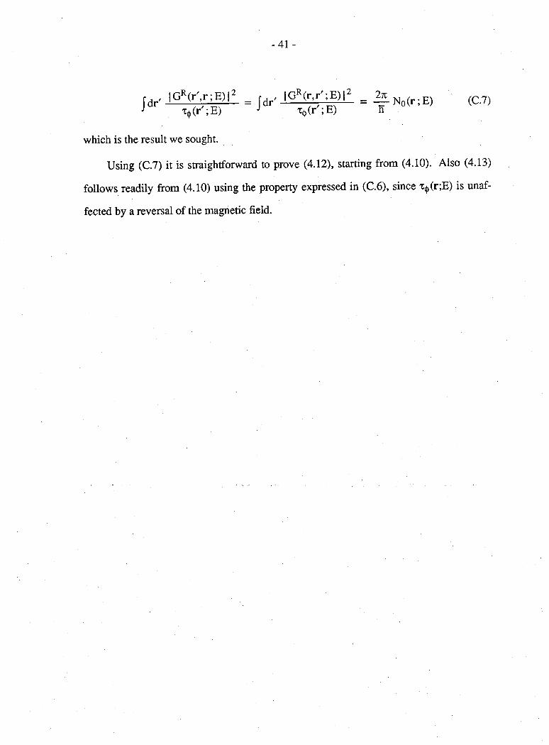
-41 -

f H r'J G V i L i M i J ^ ( r ';E )

r.,.., |GR(r,rL E ) |2 J T(i) (r';E )

^ N 0(r;E)n

(C.7)

which is the result we sought.

Using (C.7) it is straightforward to prove (4.12), starting from (4.10). Also (4.13)

follows readily from (4.10) using the property expressed in (C.6), since T^(r;E) is unaf­

fected by a reversal of the magnetic field.

Appendix D: Derivation of the Kernel from the Kubo Conductivity

The purpose of this appendix is to reproduce our expression for the kernel T(r,r')

(eqs. (5.4), (4.10)) starting from the Kubo formula for the conductivity using the Fisher-

Lee formula [2, 17]. In the Kubo formalism, the conductivity tensor a at a frequency CO

is related to the current-current correlation function [19,20],2

i©[ao(r,r';co)]ap = [Cjj(r,r';co)]ap - - ^ - 8 ( r - r ' ) 5 ap (D.1)

where n is the electron density, m is the effective mass, 5ap is the Kronecker delta and

the subscripts a, P run over x, y and z. The current-current correlation function Cjj is

defined as

- 4 2 - - .

C jj(r ,r '; ©) = -M dt ei(0t (J(r,t) J(r',0) - J(r',0) J (r ,t)) (D.2)n 0

where J(r,t) is the current density operator in the Heisenberg picture, and(* • • ) denotes

the ensemble-averaged expectation value. For convenience, we define each of the terms

composing Cjj:

C!(r,r';co) = i Jdteitot (J(r,t)J(r',0))

C2(r,r';co) = I J dt ei<ot (J(r',0) J(r,t))

The current density operator can be written as

(D.3a)

(D.3b)

J(r,t) = £ J nm(**) aft(t) aM(t) (D.4)N,M

where Jnm(r) is defined in terms of the eigenfunctions (^(r) of H0 (eq. (4.2.1)),

jNM(r) " ^ - ^ n (V^m)] (D.5)

and aft, an are the creation and annihilation operators for the eigenstate N. Substituting

(D.4) into (D.3a),

Ci(r,r';co) = X X JnmC1*) Jn'M'(rON, M N', M'

J dt elCOt (aN<t) aM(t) ajj' (O) aM'(0 )) (D.6)H o

Since N, M, N', M' are eigenstates, the expectation value on the right hand side is zero

unless N' = M and M' = N. Hence

C1(IM-^co) = X Jnm(r) JMN(r') F1(CO) ■ N,M

(DJa)

where.

I II

OOJ dt eicat (aN(t) Sn (O) )(aM(t) Sm (O) )

E o ;

= fo(eN) [ I — fo(eM)l KG) + €n - 6m +1 1

(DJb)

T] is an infinitesimal positive quantity (T] = O+). Similarly it can be shown that ; ■; '

"7 .■ .. C 2(r,r'; to) = X Jnm (f ) JMN(^)Fi(Co) N,M

(D.8a)

where F2(O1) = - f»<CM)" - f"(EN)1 Mo + En -E m + it]

(D.8b)

Substituting (D.7a,b) and (D.8a,b) into (D.2) we have

C jj(r ,r '; co) = X JnmO*) Jmn(rO Fnm(co): N,M

(D.9a)

wheref0 (Cm) ^fo(eN)

Fnm ( °) Fi F2 —NM ITco + en - eM + ITl(D.9b)

We will now rewrite FNm(cd) in a somewhat different form by proceeding as fol-

Fnm(») = Jde

-44

f0(e+lTco) 8 (e-eM+Kco) f„(e) 5 (e -eN)£ -£ n - irj e-eM+Hco+iri

Using the relation

6(x)2tti

I Ix-irj x+ir)

we obtain from (D.10),

Fnm(co) = J ^ | - [ - f0(e+Hco) G$(e) [G&(e+ITco) - G&(e+fico)]

- f 0(e) G^(e+Eco) [GA(e) - Gg(e)]]

where

G&(ei

G i m

Ie-^M +171

I

For small CO, we can write (D.l I) as

Fnm (c°) = icoaNM + bNM

where

aNM = J de UI0de

Gg1(E) G$(e)

bNM = -T- T J de f0(£) [Gn(e) Gm(e) Gn(£) Gm(^)]

Using (D.9a) and (D.l3a), we obtain from (D.l)

[G0(r,r')]ap = A + ^ - (B - S(r-r') 8ap)

(D.10)

(D.l I)

(D.12a)

(D.12b)

(D.l 3a)

(D.l 3b)

(D.13c)

(D.14a)

- 4 5 -

where A = X [ JnmC1*) ® J mn (rO lap ^nm (D.14b)N,M

B= X [Jn m (r )® JMN(rOlapt)NM (D.14c)N,M

It can be shown that A and B are both real quantities so that the real part of the conduc­

tivity is simply equal to A. From (D.13b) and (D.14b) we obtain a familiar expression

for the Kubo conductivity [Vollhardt and Wdlfl e],

a 0(r,rO = JdE8fo8E

o(r,r';E) (D.15a)

o(r,r';E) = - | - X Utm(X) 0 Jmn^O] G&(e) G$(e) (D.15b)2% N,M

So far in this appendix, we have neglected inelastic scattering; the energy Tj in eqs.

(D.12) is then a tme infinitesimal. As we have seen in Section 3, inelastic scattering

causes damping of the quasi particle propagator, which is described by including the opt­

ical potential ill/2X0^ ; E) in the defining equation for the retarded Green function (eq.

(3.2)); consequently, we modify eqs. (D.12) to

G&(e) , i . ;■e - e M+iir/2xM

Gm (£) bI

E — eM- ih/2XM

(D.16a)

(D.16b)

Since the inelastic scattering time x$(r;E) is not a constant but can vary spatially, we

have used different lifetimes Xm for the different eigenstates; in principle, these may be

obtained from the imaginary parts of the eigenenergies £m calculated using the Hamil­

tonian (H0 - ifi/2x$(r;E)). However, we assume that the imaginary potential is small

enough that we can neglect any complication due to the non-orthogonality of the

corresponding eigenfunctions <|>M(r)-

- 4 6 -

We obtain the conductivity which accounts for inelastic scattering by inserting eqs.

(D.16a,b) into eq. (D.15b),

[ Jnm (r ) ® J mn (rO Wa ap(r,r';E ) = — £ (D.17)

2k (E-£M+m/2TM)(E- £N- m / 2 x N)

We can relate this expression to T (r,r';E ) by recalling that the kernel T (r,r';E )

corresponds to the transmission coefficient between reservoirs connected to the

infinitesimal volume elements at r and r'. With this physical picture, we invoke the

Fisher-Lee formula [2,17] which links T to o. In the limit of a continuous distribution of

probes, each probe has an infinitesimal cross-section, so that from (D.17),

e2 , (Jnm(i*) * n(r) dr) (JMN(rQ * n(r') drQ _ .— T (r ,r ;E )d rd r ^ (E- e M+ ilT/2xM)(E - e N-ff i/2 TN)

where n(r) is the unit vector normal to the probe at r. But J • n is the current entering the

probe at r due to inelastic scattering which can be identified with eit/x^ (Fig. 3.3).

, _ Pnm(r) pMN(rQ/^(r iE> >E) (D 19)T r ,r ;E) " e2 N ^ (E -e M+iE/2TM)(E -e N-ilT /2TN)

where Pnm (r) = e <>n (r) <|>M (r), so that

K2T (r,r';E )

<t>N(r ) foiC1*') ^ ^mC1*) <l>M(r') 20)^ ( r ;E) X*(r'; E) £ (E -e N - i h / 2xN) ^ (E -e M+iH/2xM)

We note that the Green function can be expanded in terms of the eigenstates <t>M(r ) as

<t>M(r ) ^mCfOG (r,r ';E ) S (E -e M+ifr/2xM)

Therefore, we have obtained our previous expression for the kernel (cf. eq. (4.10)):

T (r r - E) =' t t ( r ;E )^ ( r ';E )

Eq. (5.4) for T0(r,r ) follows readily from (D.15a).

(D.21)

(D.22)

- 4 7 -

Appendix E: Derivationof theDiffusionEquation

In this Appendix our objective is to reduce the linear response equation (5.3) to the fami­liar diffusion equation (5.19) assuming a homogeneous medium in which the electrochemical potential varies slowly. First we note that in the homogeneous medium we may write (5.3) inthe form of a convolution (denoted by a *)

2 2I(r) = J dr' T(r - r ) |i(r') = x(r) * p(r) (E.l)

where T(r - r') = T08(r - r ) - T0(r - r ') (E.2)

Fourier transforming (E.l) we obtain

I(q) = T T(q) ^(q) (E.3)Now we expand t(q) in a Taylor series up to the quadratic term

T(q) = T(O) - iqj (Ti )j - q^j (T2)ij (E.4)

The coefficients in this expansion are given by the moments of t ( r - r ) in real space.

T0 = Jd p T(p) (E.5)

(Ti)j = J d p p j T(P), j = x, y, z (E.6)

I(^2)« = - j J dp Pt Pj t(p), i,j = x, ,y, z (BJ)

where we have written p for r - r . Using (5.5) and (E.2) it is evident from (E.5) that T0 =O. Also in the absence of magnetic fields T(p)=T(-p) (see eq. (5.6)) so that (Ti)j =0. The only non-zero quantities are (T2)xx = (T2)yy = (T2)zz= T2, Eq. (E.3) thus reduces to

Kq) = - (qx + qy + ^(q) (E-8)

Fourier transforming back to real space we obtain2

I(r) = - r -^ - V2 |t(r) (E.9)h

Note that I(r) is the current entering the structure through the external probes which is equal to divergence of the current density J(r) in the structure. We thus obtain the diffusion equation

(ora) n-5-=nt 3

(6'H) (J)Tl ° = f • A

- 8f r -

Fig. 2.1.

Fig. 2.2.

Fig. 2.3.

Fig. 3.1.

Fig. 3.2.

Fig. 3.3.

Fig. 3.4.

Fig. 5.1.

Fig. 5.2.

FIGURE CAPTIONS

Phase-breaking processes are assumed to be due to interaction with point

oscillators that comprise the reservoir.

One-phonon contribution to the self-energy function.

Out-scattering and in-scattering of electrons due to interaction with the reser­

voir of point oscillators.

Propagation of electron waves away from a point excitation. The argument

E has been suppressed for simplicity.

The electron density n(r;E) is obtained by superposing the individual densities

due to a continuous distribution of point sources.

M the contacts the external current I(r;E) causes a change in the electron den­

sity by An(r;E).

The contact regions are each assumed to be in local thermodynamic equili­

brium with a given electrochemical potential. The electron density n(r;E) is

free to assume any form in the rest of the structure, labeled as ‘device’.

Interpretation of successive terms in (5.12).

A weakly coupled probe connected to a device floats to a potential [Xprobe

that is a weighted average of the potential |l(r) existing within a phase­

breaking length L1J1.