Simple Method for Developing Percentile Growth Curvesfor Height and WeightRichard Ward,1 Janet Schlenker,2 and Gregory S. Anderson3*

1School of Kinesiology, Simon Fraser University, Burnaby, British Columbia V5A 1S6, Canada2Sunny Hill Health Centre for Children, Vancouver, British Columbia V5M 3E8, Canada3Kinesiology Department, University College of the Fraser Valley, Mission, British Columbia V2V 7B1, Canada

KEY WORDS children; growth; curve fitting

ABSTRACT The present paper demonstrates the easeof use of method I by Preece and Baine ([1978] Ann Hum Biol5:1–24) in generating smoothed growth curves for bothheight and weight. Using the National Center for HealthStatistics (NCHS) growth curve data, smoothed curves weredeveloped and compared to those produced using the least-squares-cubic-spline method. Based on the lower sum ofsquares and better fit of shape as indicated by residualexamination, it was concluded that the method I curve fit-

ting procedure by Preece and Baine ([1978] Ann Hum Biol5:1–24) fit centile growth curves for height and weight in2–18-year-old male and female children as well as, if notbetter than, the least-squares-cubic-spline method used indeveloping the 1979 NCHS growth curves. Further, as thispaper demonstrates, smoothed curves can be generated on adesktop computer using readily available software (theSOLVER function within Microsoft EXCEL). Am J PhysAnthropol 116:246–250, 2001. © 2001 Wiley-Liss, Inc.

The child growth charts for height and weightproduced by the National Center for Health Statis-tics (NCHS) (Hamill et al., 1979) are commonly usedby clinicians in Canada and the United States as anancillary tool to screen children for health and nu-tritional disorders. These growth curves are basedon longitudinal data for children under 36 months ofage, and on cross-sectional data for children 2–18years, and have been recommended by the WorldHealth Organization for international use since thelate 1970s. However, Cameron (1986) criticizes theuse of the terms “standards” or “norms” as indicat-ing appropriateness of the curves, inferring thatthese curves represent some kind of “ideal.” Hisargument is that they often represent the only al-ternative and may not be specific to the populationone is working with. Cameron (1986) uses the com-parison of black South African children to the NCHSgrowth curves as an example, compared to theNCHS data solely because no local standards areavailable. More recently, the NCHS growth curveswere challenged because of the nature of the originaldata (cross-sectional, American) and the analyticalmethods applied to the data in the derivation ofsmoothed curves (de Onis et al., 1997; Mei et al.,1998; Lampl and Johnson, 1998; Milani, 2000).

Clinical growth charts are required that providemore specific population standards for unique pop-ulations (i.e., ethnicity, physical or mental handi-cap). In fact, age-related growth references for gen-eral (Li et al., 1999; Cole etal., 1998; Huggins andLoesch, 1998; Wright and Royston, 1997; Leung etal., 1996: Zoppi et al., 1996), diseased (Partsch et al.,

1999; Cremers et al., 1996), and malnourished(Black and Krishanakumar, 1999; Martins and Me-nezes, 1997) populations have received much atten-tion in recent years. However, the production ofsmoothed percentile growth curves for large datasets has typically required complex distribution free(i.e., quantile regression) or parametric (i.e., expo-nential or smoothed splines) statistical procedures,using dedicated software and a computer of reason-able power (Cole et al., 1998).

It is the purpose of this paper to describe a meth-odology for the production of acceptable smoothedpercentile curves from raw data, using the Preece-Baines method I curve-fitting procedure (a modelingprocedure described by Preece and Baines, 1978).This procedure can be performed using a desktopcomputer running the readily accessible MicrosoftEXCEL 97 SR2 spreadsheet software. This method-ology is then compared to the least-squares-cubic-spline method (a mathematical curve-fitting proce-dure) employed in the production of the NCHSnorms (requiring dedicated software) to demon-strate the effectiveness of the Preece-Baines model Iagainst a known standard.

*Correspondence to: Greg Anderson, Ph.D., Kinesiology Depart-ment, University College of the Fraser Valley, Box 1000, 33700 Pren-tis Ave., Mission, British Columbia V2V 7B1, Canada.E-mail: andersong@ucfv.bc.ca

Received 21 November 2000; accepted 26 June 2001.

AMERICAN JOURNAL OF PHYSICAL ANTHROPOLOGY 116:246–250 (2001)

© 2001 WILEY-LISS, INC.

METHODS

Both the NCHS observed and smoothed percen-tiles for height and weight of boys and girls aged2–18 (Hamill et al., 1979) were entered into a Mi-crosoft EXCEL worksheet. The Preece-Baines modelI equation (Eq. 1) shown below was fit by a process ofleast sum of squares curve fitting to each of the rawpercentile curves (5th, 10th, 25th, 50th, 75th, 90th,and 95th) for both height and weight.

h 5 h1 22~h1 2 hq!

e@s0~t2q!# 1 e@s1~t2q!# (1.0)

where h is height or weight at time t, h1 is finalheight or weight, s0 and s1 are rate constants, q is atime constant, and hq is height or weight at t 5 q.

Microsoft EXCEL SOLVER function

SOLVER is a function available in EXCEL thatallows for iterative changes in a cell or cells that arelinked via an equation to a target cell. SOLVERchanges values in the linked cells in order to achievea criterion value in the target cell. The target cellcan be minimized, maximized, or targeted at anexact value. Equations from a simple straight line tothe complex Preece-Baines model can be fit by thesame basic process using the SOLVER function (formore information on SOLVER, use the Help menuin EXCEL).

Using the SOLVER function to calculate a best-fitting line requires a column of predicted values(predicted Y) generated from the equation of choice,which are placed in a column next to the actualvalues (Y). Any unknown coefficients required in theequation are entered as values in separate cells inthe worksheet and are absolutely referenced by theequation for predicting Y (thus, if any of these val-ues are changed, the predicted value of Y willchange, since they are dynamically linked). Adjacentto the predicted values, a column of residuals iscalculated (difference between actual and predict-ed). These residuals are then squared in a separatecolumn, and then a sum of these values is placed inits own cell and labeled as the sum of squares. Thebest-fitting equation through the data points is theone that has the smallest or least sum of squares,when the values of the unknowns return the lowestpossible total of squared differences. This approachcan be used to fit any line or complex curve with upto 10 unknowns. Whether fitting a straight line orsome complex curve, the least sum of squares is thecriterion of best fit.

The Preece-Baines model has five unknown val-ues and therefore has five different cells that havevalues that are referred to by the equation predict-ing Y (height or weight). Any value can be used as aninitial value in these five cells (all 1’s, for example).The SOLVER dialogue box is then invoked by menuand requires a selection of cells that can be changedby SOLVER (i.e., the five unknowns) and the cellthat should be targeted to a particular value (i.e.,

minimize the cell containing the sum of squaredresiduals). When SOLVER runs, it goes through aseries of iterations and generates a solution that fitsthe criteria. SOLVER simply goes through a processof changing the unknowns and checking whether thesum of squares has gotten smaller. When it can nolonger get the sum of squares any smaller, it reportsthat it has been minimized. SOLVER is essentially avery rapid trial-and-error iterative procedure.

The above process was repeated for each of theobserved percentile curves reported by the NCHS(Hamill et al., 1979). In order to compare to theNCHS smoothing using the cubic splining proce-dure, the NCHS smoothed percentiles were enteredinto the spreadsheet, and the corresponding sum ofsquares for their fit to the Preece-Baines percentileswas calculated.

In addition to the best-fitting curve and the leastsum of squares, the shape of the curve is also impor-tant. The ability of the Preece-Baines curves to fitthe shape of raw data curves can be appreciated byexamining the residuals plotted against age. Thisprocedure was carried out for both NCHS curvesmoothing and Preece-Baines curve smoothing. Inorder for a direct comparison of shape fit betweenNHCS and Preece-Baines smoothing, a plot of meanNCHS residuals vs. mean Preece-Baines residualswas made.

RESULTS

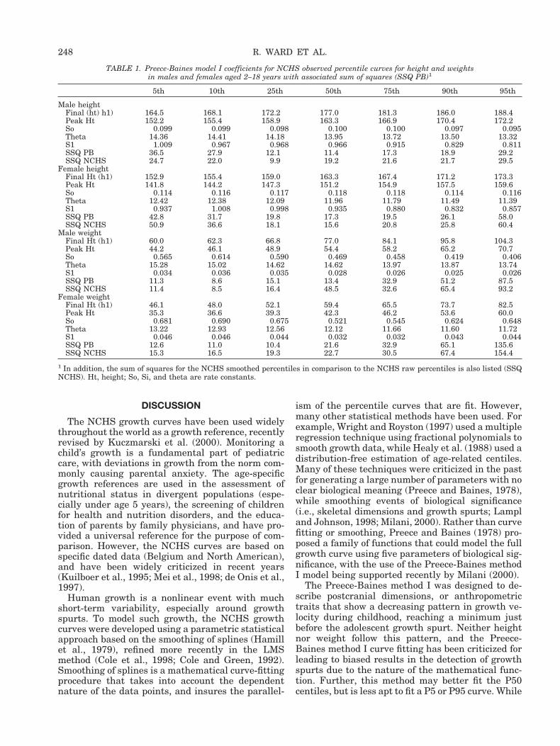
Table 1 shows the calculated Preece-Baines coef-ficients for the NCHS height and weight observedpercentile curves for boys and girls. Also displayedwere the sums of squares for the fit of the equation.The sums of squares indicate that the data werewell-fit by the Preece-Baines equation; in fact, in themajority of fits, the sum of squares for the Preece-Baines equation was lower than for the correspond-ing sum of squares for the NCHS cubic splinesmoothed. Figure 1 shows the fit of the Preece-Baines smoothed percentile curves to the observedpercentiles for boys’ height aged 2–18 years.

The Preece-Baines curve better fit the shape of theobserved percentiles in comparison to the NCHSsmoothed curves. This difference in shape is evidentby examination of the residuals. Figure 2 shows theresiduals between the observed data for males’height and the NCHS smoothed curves for all re-ported percentiles. There is a distinct pattern to theresiduals showing an underestimation around 7–8years of age, an overestimation at 10–13 years, andthen an underestimation at about 14 years. Thisillustrates the inability of the cubic splining methodto adequately follow the pattern of human growth;in Figure 3, the corresponding residuals for thePreece-Baines smoothing show a less distinct pat-tern. Figure 4 displays the resultant Preece-Bainessmoothed percentile curves for the NCHS heightand weight observed percentiles for boys and girlsaged 2–18 years.

DEVELOPING PERCENTILE GROWTH CURVES 247

DISCUSSION

The NCHS growth curves have been used widelythroughout the world as a growth reference, recentlyrevised by Kuczmarski et al. (2000). Monitoring achild’s growth is a fundamental part of pediatriccare, with deviations in growth from the norm com-monly causing parental anxiety. The age-specificgrowth references are used in the assessment ofnutritional status in divergent populations (espe-cially under age 5 years), the screening of childrenfor health and nutrition disorders, and the educa-tion of parents by family physicians, and have pro-vided a universal reference for the purpose of com-parison. However, the NCHS curves are based onspecific dated data (Belgium and North American),and have been widely criticized in recent years(Kuilboer et al., 1995; Mei et al., 1998; de Onis et al.,1997).

Human growth is a nonlinear event with muchshort-term variability, especially around growthspurts. To model such growth, the NCHS growthcurves were developed using a parametric statisticalapproach based on the smoothing of splines (Hamillet al., 1979), refined more recently in the LMSmethod (Cole et al., 1998; Cole and Green, 1992).Smoothing of splines is a mathematical curve-fittingprocedure that takes into account the dependentnature of the data points, and insures the parallel-

ism of the percentile curves that are fit. However,many other statistical methods have been used. Forexample, Wright and Royston (1997) used a multipleregression technique using fractional polynomials tosmooth growth data, while Healy et al. (1988) used adistribution-free estimation of age-related centiles.Many of these techniques were criticized in the pastfor generating a large number of parameters with noclear biological meaning (Preece and Baines, 1978),while smoothing events of biological significance(i.e., skeletal dimensions and growth spurts; Lampland Johnson, 1998; Milani, 2000). Rather than curvefitting or smoothing, Preece and Baines (1978) pro-posed a family of functions that could model the fullgrowth curve using five parameters of biological sig-nificance, with the use of the Preece-Baines methodI model being supported recently by Milani (2000).

The Preece-Baines method I was designed to de-scribe postcranial dimensions, or anthropometrictraits that show a decreasing pattern in growth ve-locity during childhood, reaching a minimum justbefore the adolescent growth spurt. Neither heightnor weight follow this pattern, and the Preece-Baines method I curve fitting has been criticized forleading to biased results in the detection of growthspurts due to the nature of the mathematical func-tion. Further, this method may better fit the P50centiles, but is less apt to fit a P5 or P95 curve. While

TABLE 1. Preece-Baines model I coefficients for NCHS observed percentile curves for height and weightsin males and females aged 2–18 years with associated sum of squares (SSQ PB)1

5th 10th 25th 50th 75th 90th 95th

Male heightFinal (ht) h1) 164.5 168.1 172.2 177.0 181.3 186.0 188.4Peak Ht 152.2 155.4 158.9 163.3 166.9 170.4 172.2So 0.099 0.099 0.098 0.100 0.100 0.097 0.095Theta 14.36 14.41 14.18 13.95 13.72 13.50 13.32S1 1.009 0.967 0.968 0.966 0.915 0.829 0.811SSQ PB 36.5 27.9 12.1 11.4 17.3 18.9 29.2SSQ NCHS 24.7 22.0 9.9 19.2 21.6 21.7 29.5

Female heightFinal Ht (h1) 152.9 155.4 159.0 163.3 167.4 171.2 173.3Peak Ht 141.8 144.2 147.3 151.2 154.9 157.5 159.6So 0.114 0.116 0.117 0.118 0.118 0.114 0.116Theta 12.42 12.38 12.09 11.96 11.79 11.49 11.39S1 0.937 1.008 0.998 0.935 0.880 0.832 0.857SSQ PB 42.8 31.7 19.8 17.3 19.5 26.1 58.0SSQ NCHS 50.9 36.6 18.1 15.6 20.8 25.8 60.4

Male weightFinal Ht (h1) 60.0 62.3 66.8 77.0 84.1 95.8 104.3Peak Ht 44.2 46.1 48.9 54.4 58.2 65.2 70.7So 0.565 0.614 0.590 0.469 0.458 0.419 0.406Theta 15.28 15.02 14.62 14.62 13.97 13.87 13.74S1 0.034 0.036 0.035 0.028 0.026 0.025 0.026SSQ PB 11.3 8.6 15.1 13.4 32.9 51.2 87.5SSQ NCHS 11.4 8.5 16.4 48.5 32.6 65.4 93.2

Female weightFinal Ht (h1) 46.1 48.0 52.1 59.4 65.5 73.7 82.5Peak Ht 35.3 36.6 39.3 42.3 46.2 53.6 60.0So 0.681 0.690 0.675 0.521 0.545 0.624 0.648Theta 13.22 12.93 12.56 12.12 11.66 11.60 11.72S1 0.046 0.046 0.044 0.032 0.032 0.043 0.044SSQ PB 12.6 11.0 10.4 21.6 32.9 65.1 135.6SSQ NCHS 15.3 16.5 19.3 22.7 30.5 67.4 154.4

1 In addition, the sum of squares for the NCHS smoothed percentiles in comparison to the NCHS raw percentiles is also listed (SSQNCHS). Ht, height; So, Si, and theta are rate constants.

248 R. WARD ET AL.

this was evident with larger sum of squares for P5and P95 centile curves in the present analysis, itwas concluded that the Preece-Baines smoothingprovided a better fit to the observed percentiles thanthe original cubic splining methodology (based onthe evidence of lower sum of squares and bettershape fit indicated by residual examination). Thisresult is similar to that of Milani (2000), who re-viewed the use of kinetic models to describe humangrowth in healthy children and children with patho-logically impaired growth, suggesting that thePreece-Baines method I model may function well inboth populations.

While this paper could have used any number ofcurve fitting procedures and/or models, the presentpaper demonstrates the ease of use of method I byPreece and Baine (1978) in generating smoothedgrowth curves for both height and weight, using theNCHS growth curve data (Hamill et al., 1979). Inaddition, with the method of iterative curve fittingusing Solver in Microsoft EXCEL described here,other workers may easily produce smoothed percen-tile curves for local growth norms easily, and with-out dedicated software. In doing so, we might even-tually reach the goal of having adequate specificpopulation standards to service the needs of all chil-dren in the world.

Fig. 1. Preece-Baines smoothed percentiles for height in USboys aged 2–18 years, with NCHS reported observed percentiles.

Fig. 2. Plot of residuals between NCHS smoothed percentilesvs. observed percentiles for height in US boys aged 2–18 years.

Fig. 3. Plot of residuals between Preece-Baines smoothed per-centiles vs. observed percentiles for height in US boys aged 2–18years.

Fig. 4. Preece-Baines smoothed percentiles of NCHS reportedheight and weight in US boys and girls aged 2–18 years.

DEVELOPING PERCENTILE GROWTH CURVES 249

AUTHOR’S NOTE

For more information on the use of the MicrosoftEXCEL SOLVER function, consult the Help func-tion within EXCEL, or contact Dr. Richard Ward atrichard_ward@sfu.ca.

LITERATURE CITED

Black MM, Krishanakumar A. 1999. Predicting longitudinalgrowth curves of height and weight using ecological factors forchildren with and without early growth deficiency. J Nutr 129:539–543.

Cameron N. 1986. Standards for human growth—their construc-tion and use. S Afr Med J 70:422–425.

Cole TJ. 1996. A critique of the NCHS weight for height standard.Hum Biol 57:183–190.

Cole TJ, Green PJ. 1992. Smoothing reference centile curves: theLMS method and penalized likelihood. Stat Med 11:1305–1319.

Cole TJ, Freeman JV, Preece MA. 1998. British 1990 growthreference centiles for weight, height, body mass index and headcircumference fitted by maximum penalized likelihood. StatMed 17:407–429.

Cremers MJ, van der Tweel I, Boersma B, Wit JM, Zonderland M,1996. Growth curves of Dutch children with Down’s syndrome.J Intellect Disabil Res 40:412–420.

de Onis M, Garza C, Habicht JP. 1997. Time for a new growthreference. Pediatrics 100:8.

Hamill PVV, Dridzd TA, Johnson CL, Reed RB, Roche AF, MooreWM. 1979. Physical growth: National Center for Health Sta-tistics percentiles. Am J Clin Nutr 32:607–629.

Healy MJR, Rasbash J, Yang M. 1988. Distribution-free estima-tion of age-related centiles. Ann Hum Biol 15:17–22.

Huggins RM, Loesch DZ. 1998. On the analysis of mixed longitu-dinal growth data. Biometrics 54:583–595.

Kuczmarski RJ, Ogden CL, Grummer-Strawn LM, Flegal KM,Guo SS, Wei R, Mei Z, Curtin LR, Roche AF, Johnson CL. 2000.CDC growth charts: United States. Adv Data 314:1–28 [re-vised].

Kuilboer MM, Wilson DM, Musen MA, Wit JM. 1995. CALIPER:individualized-growth curves for the monitoring of children’sgrowth. Medinfo 8:1686.

Lampl M, Johnson ML. 1998. Wrinkles induced by use of smooth-ing procedures applied to serial growth data. Ann Hum Biol25:187–202.

Leung SS, Lau JT, Tse LY, Oppenheimer SJ. 1996. Weight-for-age and weight-for-height references for Hong Kong childrenfrom birth to 18 years. J Paediatr Child Health 32:103–109.

Li H, Leung SSF, Lam PKW, Zhang X, Chen XX, Wang SL. 1999.Height and weight percentile curves for Beijing children andadolescents 0–18 years, 1995. Ann Hum Biol 26:457–471.

Martins SJ, Menezes RC. 1997. A mathematical approach forestimating reference values for weight-for-age, weight-for-height and height-for-age. Growth Dev Aging 61:3–10.

Mei Z, Yip R, Grummer Strawn LM, Trowbridge FL. 1998. De-velopment of a research child growth reference and its compar-ison with the current international growth reference. ArchPediatr Adolesc Med 152:471–479.

Milani S. 2000. Kinetic models for normal and impaired growth.Ann Hum Biol 27:1–18.

Partsch CJ, Dreyer G, Gosch A, Winter M, Schneppenheim R,Wessel A, Pankau R. 1999. Longitudinal evaluation of growth,puberty, and bone maturation in children with Williams syn-drome. J Pediatr 134:82–89.

Preece MA, Baines MJ. 1978. A new family of mathematicalmodels describing the human growth curve. Ann Hum Biol5:1–24.

Wright EM, Royston P. 1997. Simplified estimation of age-specificreference intervals for skewed data. Stat Med 16:2785–2803.

Zoppi G, Bressan F, Luciano A. 1996. Height and weight refer-ence charts for children aged 2–18 years from Verona, Italy.Eur J Clin Nutr 50:462–468.

250 R. WARD ET AL.