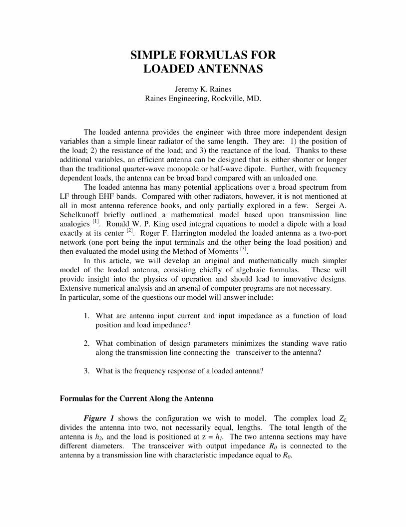
SIMPLE FORMULAS FOR

LOADED ANTENNAS

Jeremy K. Raines

Raines Engineering, Rockville, MD.

The loaded antenna provides the engineer with three more independent design

variables than a simple linear radiator of the same length. They are: 1) the position of

the load; 2) the resistance of the load; and 3) the reactance of the load. Thanks to these

additional variables, an efficient antenna can be designed that is either shorter or longer

than the traditional quarter-wave monopole or half-wave dipole. Further, with frequency

dependent loads, the antenna can be broad band compared with an unloaded one.

The loaded antenna has many potential applications over a broad spectrum from

LF through EHF bands. Compared with other radiators, however, it is not mentioned at

all in most antenna reference books, and only partially explored in a few. Sergei A.

Schelkunoff briefly outlined a mathematical model based upon transmission line

analogies [1]

. Ronald W. P. King used integral equations to model a dipole with a load

exactly at its center [2]

. Roger F. Harrington modeled the loaded antenna as a two-port

network (one port being the input terminals and the other being the load position) and

then evaluated the model using the Method of Moments [3]

.

In this article, we will develop an original and mathematically much simpler

model of the loaded antenna, consisting chiefly of algebraic formulas. These will

provide insight into the physics of operation and should lead to innovative designs.

Extensive numerical analysis and an arsenal of computer programs are not necessary.

In particular, some of the questions our model will answer include:

1. What are antenna input current and input impedance as a function of load

position and load impedance?

2. What combination of design parameters minimizes the standing wave ratio

along the transmission line connecting the transceiver to the antenna?

3. What is the frequency response of a loaded antenna?

Formulas for the Current Along the Antenna

Figure 1 shows the configuration we wish to model. The complex load ZL

divides the antenna into two, not necessarily equal, lengths. The total length of the

antenna is h2, and the load is positioned at z = h1. The two antenna sections may have

different diameters. The transceiver with output impedance R0 is connected to the

antenna by a transmission line with characteristic impedance equal to R0.

Figure 1. The loaded antenna provides three more independent design variables (load position, load resistance and load reactance) than an unloaded antenna of the same length. Shown are the essential geometry and design parameters.

The current on each section of the antenna is the superposition of forward and

reverse traveling waves. The current on the upper section is:

The current on the lower section is:

In Equation 1, we have arbitrarily set the complex amplitude of the forward traveling

wave to unity without loss of generality. In Equations 1 and 2, the wave number is:

Where λ is the wavelength, f is is the frequency, and c is the velocity of light.

In a recent book [4]

, the author used the analogy between antennas and

transmission lines to write down simple formulas for traveling waves of voltage

propagating along the antenna. On the upper section, the voltage is:

On the lower section, the voltage is:

jkzjkz eezI Γ−= −)(2

jkz

R

jkz

FeIeIzI += −

)(1

c

fk

π

λ

π 22==

( )jkzjkzeeZzV Γ+= −

022)(

)1(

)2(

)3(

)4(

In the same book, the author derived simple formulas for the characteristic impedances

[5]

:

In Equation 6, η is the impedance of free space and ai is the radius of the antenna section.

The quasi-static wave number k’ is [6]

:

In Equation 7, γ is Euler’s constant (577215…).

In a recent paper [7]

, the author expanded the analogy between antennas and

transmission lines and derived a simple yet accurate formula for the reflection coefficient

Γ in Equation 8:

In Equation 8, the complex impedance Zs models the antenna end effect at the tip of the

upper section. In many antenna models, Zs is approximated as an open circuit; however,

for lengths greater than a quarter wavelength, this approximation leads to infinity as the

value for antenna input impedance at integer multiples of half wavelength. While this

value is a good zeroth order approximation, it is of little practical use. Instead, a better

and more useful representation for Zs is the parallel combination of the radiation

resistance of a virtual annular slot and the antenna end capacitance:

In Equation 9, the radiation resistance Rs of the virtual annular slot is approximately

112.5 Ω for any antenna radius. The reactance of the end capacitance is:

)()(011

jkz

R

jkz

FeIeIZzV −= −

( ) 2,1'ln2

0=−= iakZ

iiπ

η

)5(

)6(

ke

k2

'γ

=

s

skhj

ZZ

ZZe

+

−=Γ −

02

022 2

s

s

sRjX

jXRZ

+=

216

1

afX

επ−=

)7(

)8(

)9(

)10(

)7(

In Equation 10, ε is the permittivity of free space.

So far, we have uniquely specified all of the variables in the formulas except for

the complex amplitudes IF and IR in Equation 2. To determine those, we need two

independent equations, and those are boundary conditions at the load. First, we require

that the currents on the upper and lower sections be continuous through the load:

Second, we require that the voltage and current at the load satisfy the constitutive law of

the impedance ZL:

If we apply Equations 1 and 2 to Equations 11 and 12, then, after some algebra, we obtain

formulas for the complex amplitudes of the currents on the lower section. The amplitude

of the forward traveling wave is:

The amplitude of the reverse or reflected traveling wave is:

In Equations 13 and 14, the forward traveling wave function is:

)()(1112

hIhI =

LZhIhVhV )()()(

111211=−

( )( ) ( )

F

RFRFL

FZ

ZZZI

ψ

ψψψψ

01

0201

2

Γ++Γ−+=

( )( ) ( )

R

RFRFL

R

F

RZ

ZZZI

ψ

ψψψψ

ψ

ψ

01

0201

2

Γ++Γ−+−Γ−=

1jkh

Fe

−=ψ

)11(

)12(

)13(

)14(

)15(

The reverse traveling wave function is:

Antenna Input Current and Input Reactance

Using the derivations of the previous section, it is a straight forward procedure to

obtain formulas for the input current and reactance of the antenna. From Equation 2, the

input current is:

The terms on the right side of Equation 17 can be evaluated using Equations 13 and 14.

From Equation 5, the antenna input voltage is:

The input impedance follows immediately from Equations 17 and 18:

Equation 19 does not include the contribution from radiation resistance. We will derive a

formula for that in the next section. If the load ZL has a resistive component, however,

then that will show up in Zin. Otherwise, Zin will be completely imaginary, or reactive. In

any case, the antenna input reactance is the imaginary part of the right side of Equation

19:

1jkh

Re=ψ

RFinIIII +== )0(

1

)16(

)17(

( )RFin

IIZVV −==011

)0(

RF

RF

in

in

inII

IIZ

I

VZ

+

−==

01

2Im

201

π≥

+

−= kh

II

IIZX

RF

RF

in

)18(

)19(

)20(

For antennas shorter than a quarter wavelength, a self contained formula is just as

accurate and more convenient:

In Equation 21,

Equations 20 and 21 join seamlessly at kh2 = π/2.

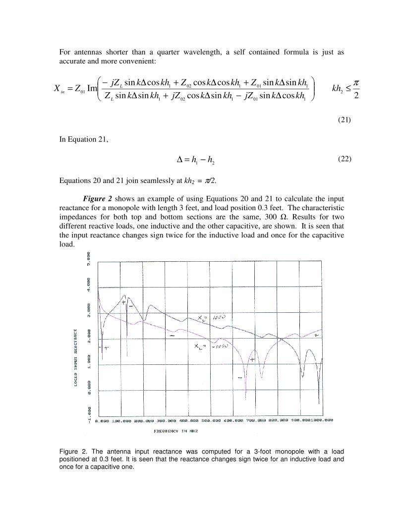
Figure 2 shows an example of using Equations 20 and 21 to calculate the input

reactance for a monopole with length 3 feet, and load position 0.3 feet. The characteristic

impedances for both top and bottom sections are the same, 300 Ω. Results for two

different reactive loads, one inductive and the other capacitive, are shown. It is seen that

the input reactance changes sign twice for the inductive load and once for the capacitive

load.

Figure 2. The antenna input reactance was computed for a 3-foot monopole with a load positioned at 0.3 feet. It is seen that the reactance changes sign twice for an inductive load and once for a capacitive one.

2cossinsincossinsin

sinsincoscoscossinIm

2

1011021

1011021

01

π≤

∆−∆+∆

∆+∆+∆−= kh

khkjZkhkjZkhkZ

khkZkhkZkhkjZZX

L

L

in

21hh −=∆

)21(

)22(

Radiated Electromagnetic Field and Radiation Resistance

The current distribution described by Equations 1 and 2 readily determines the

radiated electric field [8]

:

In equation 23, the vertical radiation characteristic is:

Equation 24 can be evaluated exactly in terms of simple functions [9]

; however, with

modern desktop computers, it is quickly evaluated numerically as well. The integration

ranges over both the upper and lower sections of the antenna.

From the radiated electric field, the radiated power density, or Poynting vector, is

readily obtained:

and also the total radiated power:

For vertical or z-directed wires, using Equations 23 to 25, Equation 26 becomes:

Finally, the input radiation resistance is:

)(4

sinθ

π

θηθ

Fr

ejE

jkr−

=

( )∫+=

kl

jkzkzdezIF

θθ cos)()(

ηθ

2

ES =

∫∫=ππ

θθϕ0

2

2

0

sin dSrdP

( )∫=π

θθθη

0

22sin2

FdP

( )∫==π

θθθη

0

22

22sin

2Fd

II

PR

inin

in

)23(

)242(

)(23(

)264(

)275(

)276(

)23(

)24(

)25(

)26(

)27(

)28(

Equation 17 is used to compute Iin in Equation 28.

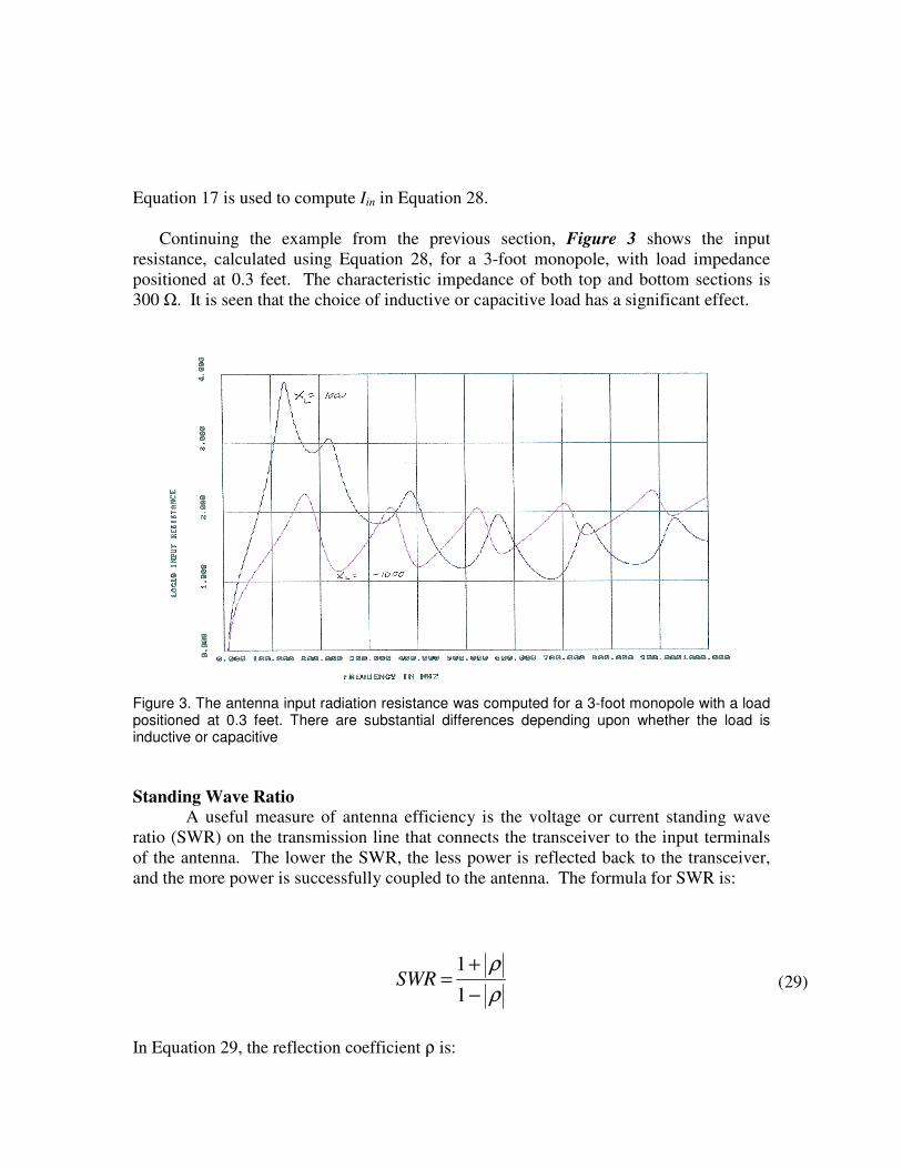
Continuing the example from the previous section, Figure 3 shows the input

resistance, calculated using Equation 28, for a 3-foot monopole, with load impedance

positioned at 0.3 feet. The characteristic impedance of both top and bottom sections is

300 Ω. It is seen that the choice of inductive or capacitive load has a significant effect.

Figure 3. The antenna input radiation resistance was computed for a 3-foot monopole with a load positioned at 0.3 feet. There are substantial differences depending upon whether the load is inductive or capacitive

Standing Wave Ratio

A useful measure of antenna efficiency is the voltage or current standing wave

ratio (SWR) on the transmission line that connects the transceiver to the input terminals

of the antenna. The lower the SWR, the less power is reflected back to the transceiver,

and the more power is successfully coupled to the antenna. The formula for SWR is:

In Equation 29, the reflection coefficient ρ is:

ρ

ρ

−

+=

1

1SWR )29(

In Equation 30, R0 is the characteristic impedance and l is the length of the transmission

line illustrated in Figure 1. The antenna input impedance ZA is:

In Equation 31, Rin and Xin are calculated using Equations 28 and 20, respectively.

The standing wave ratio is often expressed in terms of decibels, in which case Equation

29 is replaced by:

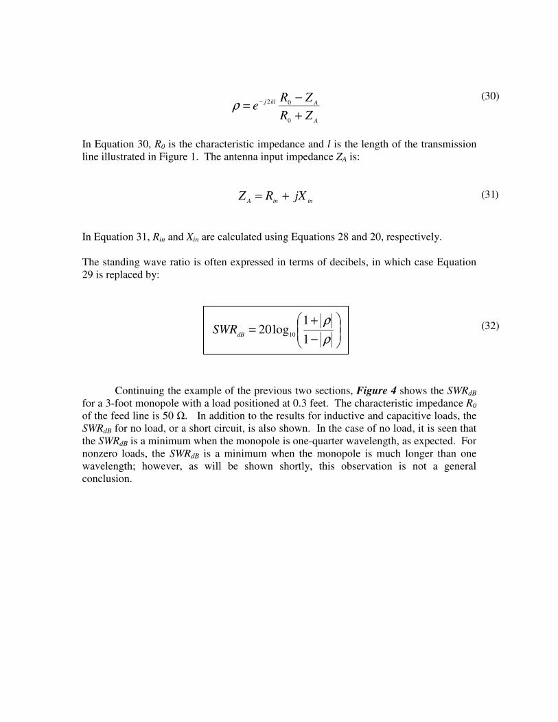
Continuing the example of the previous two sections, Figure 4 shows the SWRdB

for a 3-foot monopole with a load positioned at 0.3 feet. The characteristic impedance R0

of the feed line is 50 Ω. In addition to the results for inductive and capacitive loads, the

SWRdB for no load, or a short circuit, is also shown. In the case of no load, it is seen that

the SWRdB is a minimum when the monopole is one-quarter wavelength, as expected. For

nonzero loads, the SWRdB is a minimum when the monopole is much longer than one

wavelength; however, as will be shown shortly, this observation is not a general

conclusion.

A

Aklj

ZR

ZRe

+

−= −

0

02ρ

ininAjXRZ +=

−

+=

ρ

ρ

1

1log20

10dBSWR

)30(

)31(

)32(

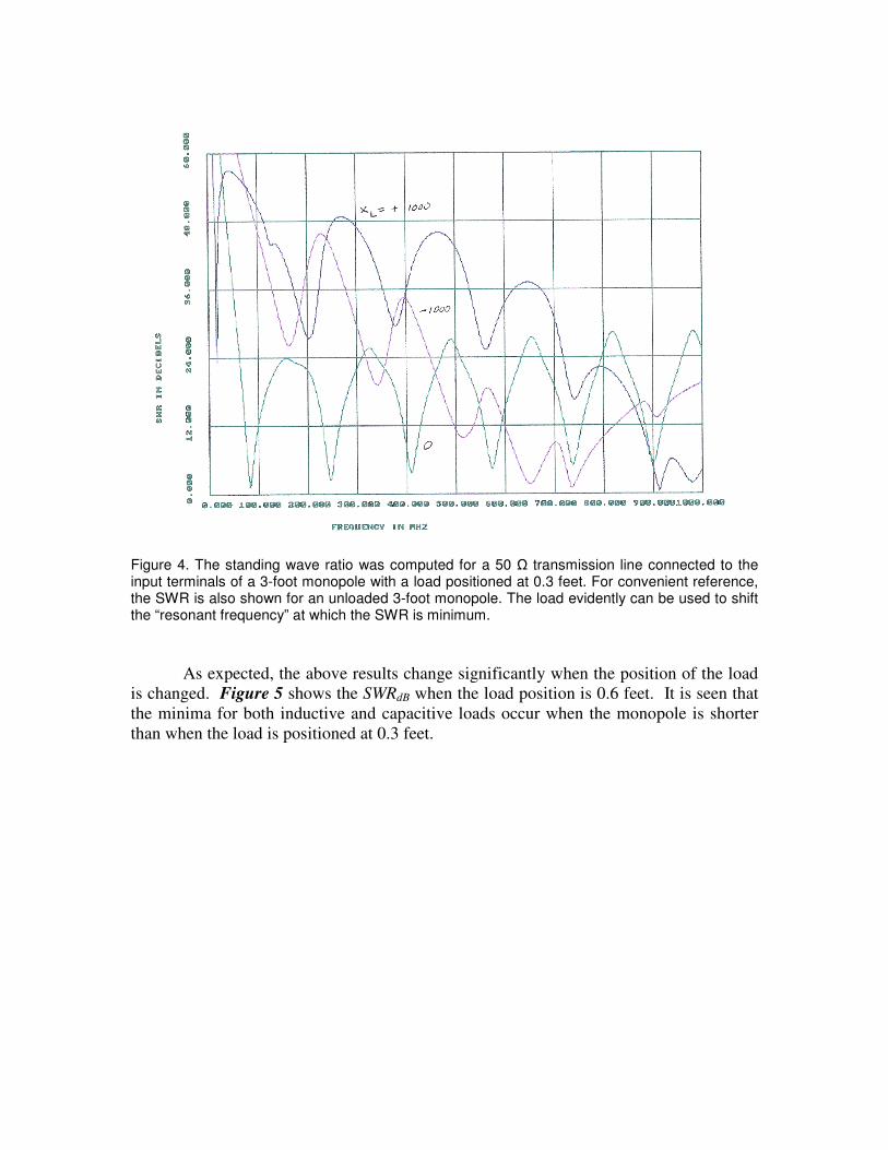
Figure 4. The standing wave ratio was computed for a 50 Ω transmission line connected to the input terminals of a 3-foot monopole with a load positioned at 0.3 feet. For convenient reference, the SWR is also shown for an unloaded 3-foot monopole. The load evidently can be used to shift the “resonant frequency” at which the SWR is minimum.

As expected, the above results change significantly when the position of the load

is changed. Figure 5 shows the SWRdB when the load position is 0.6 feet. It is seen that

the minima for both inductive and capacitive loads occur when the monopole is shorter

than when the load is positioned at 0.3 feet.

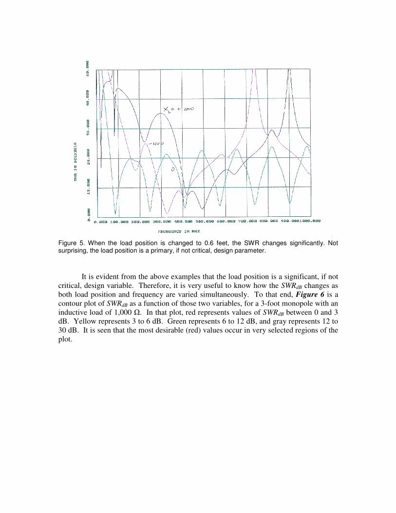
Figure 5. When the load position is changed to 0.6 feet, the SWR changes significantly. Not surprising, the load position is a primary, if not critical, design parameter.

It is evident from the above examples that the load position is a significant, if not

critical, design variable. Therefore, it is very useful to know how the SWRdB changes as

both load position and frequency are varied simultaneously. To that end, Figure 6 is a

contour plot of SWRdB as a function of those two variables, for a 3-foot monopole with an

inductive load of 1,000 Ω. In that plot, red represents values of SWRdB between 0 and 3

dB. Yellow represents 3 to 6 dB. Green represents 6 to 12 dB, and gray represents 12 to

30 dB. It is seen that the most desirable (red) values occur in very selected regions of the

plot.

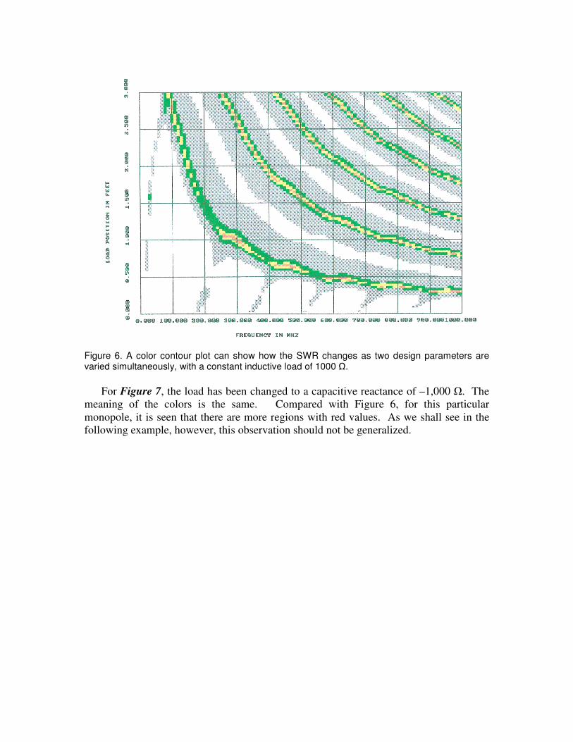
Figure 6. A color contour plot can show how the SWR changes as two design parameters are varied simultaneously, with a constant inductive load of 1000 Ω.

For Figure 7, the load has been changed to a capacitive reactance of –1,000 Ω. The

meaning of the colors is the same. Compared with Figure 6, for this particular

monopole, it is seen that there are more regions with red values. As we shall see in the

following example, however, this observation should not be generalized.

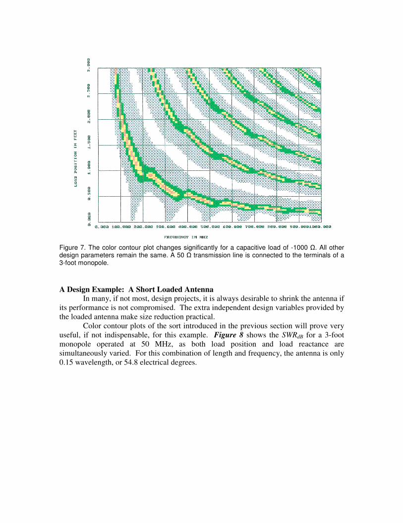
Figure 7. The color contour plot changes significantly for a capacitive load of -1000 Ω. All other design parameters remain the same. A 50 Ω transmission line is connected to the terminals of a 3-foot monopole.

A Design Example: A Short Loaded Antenna

In many, if not most, design projects, it is always desirable to shrink the antenna if

its performance is not compromised. The extra independent design variables provided by

the loaded antenna make size reduction practical.

Color contour plots of the sort introduced in the previous section will prove very

useful, if not indispensable, for this example. Figure 8 shows the SWRdB for a 3-foot

monopole operated at 50 MHz, as both load position and load reactance are

simultaneously varied. For this combination of length and frequency, the antenna is only

0.15 wavelength, or 54.8 electrical degrees.

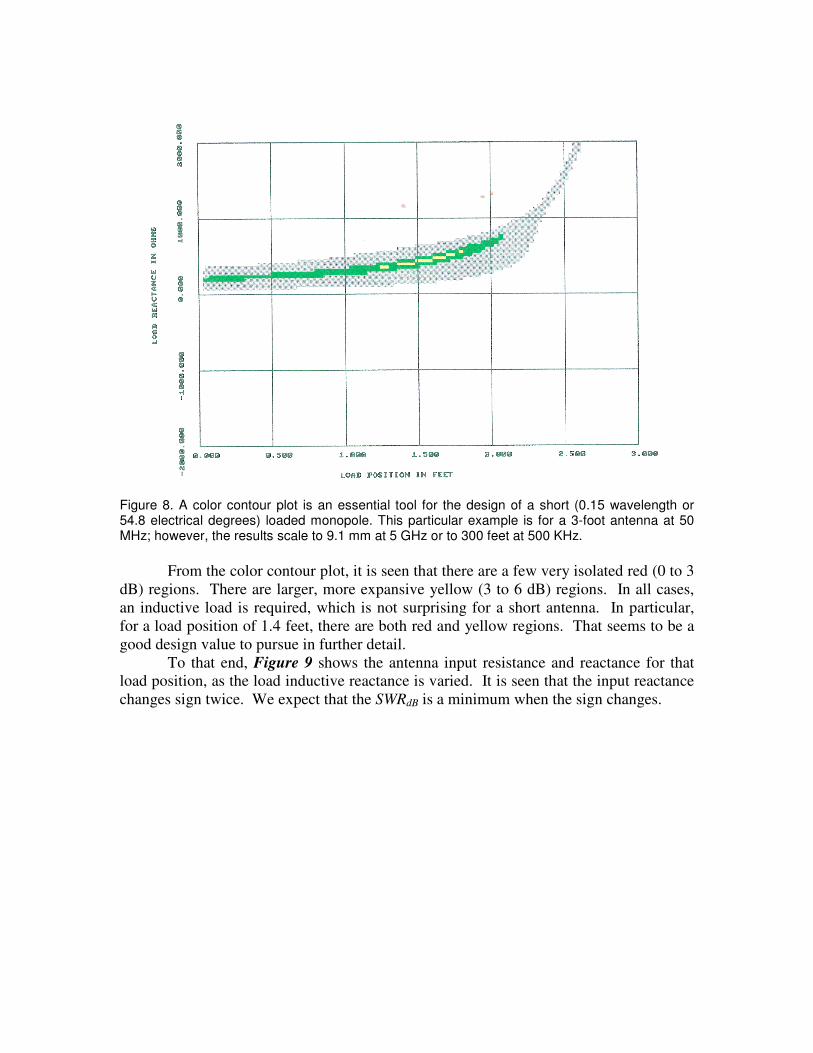
Figure 8. A color contour plot is an essential tool for the design of a short (0.15 wavelength or 54.8 electrical degrees) loaded monopole. This particular example is for a 3-foot antenna at 50 MHz; however, the results scale to 9.1 mm at 5 GHz or to 300 feet at 500 KHz.

From the color contour plot, it is seen that there are a few very isolated red (0 to 3

dB) regions. There are larger, more expansive yellow (3 to 6 dB) regions. In all cases,

an inductive load is required, which is not surprising for a short antenna. In particular,

for a load position of 1.4 feet, there are both red and yellow regions. That seems to be a

good design value to pursue in further detail.

To that end, Figure 9 shows the antenna input resistance and reactance for that

load position, as the load inductive reactance is varied. It is seen that the input reactance

changes sign twice. We expect that the SWRdB is a minimum when the sign changes.

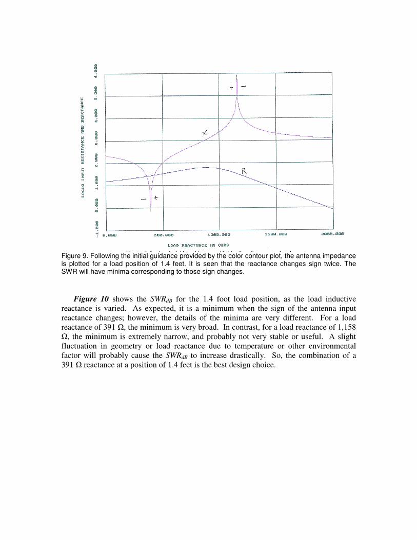
Figure 9. Following the initial guidance provided by the color contour plot, the antenna impedance is plotted for a load position of 1.4 feet. It is seen that the reactance changes sign twice. The SWR will have minima corresponding to those sign changes.

Figure 10 shows the SWRdB for the 1.4 foot load position, as the load inductive

reactance is varied. As expected, it is a minimum when the sign of the antenna input

reactance changes; however, the details of the minima are very different. For a load

reactance of 391 Ω, the minimum is very broad. In contrast, for a load reactance of 1,158

Ω, the minimum is extremely narrow, and probably not very stable or useful. A slight

fluctuation in geometry or load reactance due to temperature or other environmental

factor will probably cause the SWRdB to increase drastically. So, the combination of a

391 Ω reactance at a position of 1.4 feet is the best design choice.

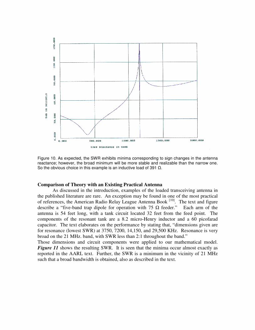
Figure 10. As expected, the SWR exhibits minima corresponding to sign changes in the antenna reactance; however, the broad minimum will be more stable and realizable than the narrow one. So the obvious choice in this example is an inductive load of 391 Ω.

Comparison of Theory with an Existing Practical Antenna

As discussed in the introduction, examples of the loaded transceiving antenna in

the published literature are rare. An exception may be found in one of the most practical

of references, the American Radio Relay League Antenna Book [10]

. The text and figure

describe a “five-band trap dipole for operation with 75 Ω feeder.” Each arm of the

antenna is 54 feet long, with a tank circuit located 32 feet from the feed point. The

components of the resonant tank are a 8.2 micro-Henry inductor and a 60 picofarad

capacitor. The text elaborates on the performance by stating that, “dimensions given are

for resonance (lowest SWR) at 3750, 7200, 14,150, and 29,500 KHz. Resonance is very

broad on the 21 MHz. band, with SWR less than 2:1 throughout the band.”

Those dimensions and circuit components were applied to our mathematical model.

Figure 11 shows the resulting SWR. It is seen that the minima occur almost exactly as

reported in the AARL text. Further, the SWR is a minimum in the vicinity of 21 MHz

such that a broad bandwidth is obtained, also as described in the text.

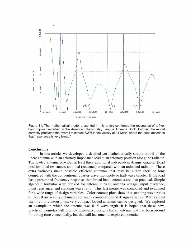
Figure 11. The mathematical model presented in this article confirmed the resonance of a five-band dipole described in the American Radio relay League Antenna Book. Further, the model correctly predicted the overall minimum SWR in the vicinity of 21 MHz, where the book describes that “resonance is very broad.”

Conclusions

In this article, we developed a detailed yet mathematically simple model of the

linear antenna with an arbitrary impedance load at an arbitrary position along the radiator.

The loaded antenna provides at least three additional independent design variables (load

position, load resistance, and load reactance) compared with an unloaded radiator. These

extra variables make possible efficient antennas that may be either short or long

compared with the conventional quarter-wave monopole or half-wave dipole. If the load

has a prescribed frequency response, then broad band antennas are also practical. Simple

algebraic formulas were derived for antenna current, antenna voltage, input reactance,

input resistance, and standing wave ratio. This last metric was computed and examined

for a wide range of design variables. Color contour plots show that standing wave ratios

of 0-3 dB are readily obtainable for many combinations of design variables. With careful

use of color contour plots, very compact loaded antennas can be designed. We explored

an example in which the antenna was 0.15 wavelength. It is hoped that these new,

practical, formulas will promote innovative designs for an antenna that has been around

for a long time conceptually, but that still has much unexplored potential.

Acknowledgment

The author thanks Mr. Ron Nott, of Nott Limited, Farmington, New Mexico for

suggesting the standing wave ratio as a convenient and meaningful measure of antenna

performance.

References

1 S. A. Schelkunoff and H. T., Friis, “Antennas Theory and Practice,” John

Wiley & Sons, Hoboken, NJ. 1952, pp. 246-247.

2 R. W. P. King, “The Theory of Linear Antennas,” Harvard University

Press, Cambridge, MA, 1956, pp. 461-501.

3 R. F. Harrington, “Field Computation by Moment Methods,” The

Macmillan Company, New York, NY., 1968, pp. 110-115.

4 J. K. Raines, “The Folded Unipole Antenna Theory and Applications,”

McGraw-Hill, New York, NY., 2007, pp. 11-12.

5 Ibid., p. 225-32.

6 Ibid., p. 231.

7 J. K. Raines, “The Virtual Outer Conductor for Linear Antennas,” The

Microwave Journal, Vol. 52, No. 1, January, 2009, pp.

8 E. A. Wolff, “Antenna Analysis,” John Wiley & Sons, Hoboken, NJ.,1966,

p. 77.

9 J. K. Raines, “The Folded Unipole Antenna Theory and Applications,”

McGraw-Hill, New York, NY., 2007, p. 45.

10 “The ARRL Antenna Book,” Newington, CN., 1964, p. 194.

Biography

Jeremy Keith Raines received his BS degree in electrical science and engineering from

MIT, his MS degree in applied physics from Harvard University and his Ph.D. degree in

electromagnetics from MIT. He is a registered professional engineer in the state of

Maryland. Since 1972, he has been a consulting engineer in electromagnetics. Antennas

designed by him span the spectrum from ELF through SHF, and they may be found on

satellites deep in space, on ships, on submarines, on aircraft, and at a variety of terrestrial

sites. He may be contacted at www.rainesengineering.com.