Simple Efficient Solutions for Semidefinite Programming

Henry Wolkowicz ∗

October 4, 2001

University of WaterlooDepartment of Combinatorics & Optimization

Waterloo, Ontario N2L 3G1, CanadaResearch Report CORR 2001-49 1

Key words: Semidefinite Programming, large sparse problems, inexact Gauss-Newtonmethod, preconditioned conjugate gradients, optimal diagonal preconditioner, Max-Cut Prob-lem.

Abstract

This paper provides a simple approach for solving a semidefinite program, SDP.As is common with many other approaches, we apply a primal-dual method that usesthe perturbed optimality equations for SDP, Fµ(X, y, Z) = 0, where X, Z are n × n

symmetric matrices and y ∈ ℜm. However, as in Kruk et al [19], we look at this as anoverdetermined system of nonlinear (bilinear) equations on vectors X, y, Z which hasa zero residual at optimality. We do not use any symmetrization on this system. Thatthe vectors X, Z are symmetric matrices is ignored. What is different in this paper is apreprocessing step that results in one single, well-conditioned, overdetermined bilinearequation. We do not form a Schur complement form for the linearized system. Inaddition, asymptotic q-quadratic convergence is obtained with a crossover approachthat switches to affine scaling without maintaining the positive (semi)definiteness ofX and Z. This results in a marked reduction in the number and the complexity of theiterations.

We use the long accepted method for nonlinear least squares problems, the Gauss-Newton method. For large sparse data, we use an inexact Gauss-Newton approachwith a preconditioned conjugate gradient method applied directly on the linearizedequations in matrix space. This does not require any operator formations into a Schurcomplement system or matrix representations of linear operators.

∗Research supported by The Natural Sciences and Engineering Research Council of Canada. E-mailhwolkowicz@uwaterloo.ca

1A modified version of this paper, Semidefinite Programming and Some Closest Matrix Approximation

Problems, was presented at the 1st Annual McMaster Optimization Conference (MOPTA 01), August 2-4,2001 Hamilton, Ontario.

1 URL for paper and MATLAB programs:http://orion.math.uwaterloo.ca/˜hwolkowi/henry/reports/ABSTRACTS.html

1

To illustrate the approach, we apply it to the well known SDP relaxation of theMax-Cut problem. The cost of an iteration consists almost entirely in the solution

of a (generally well-conditioned) least squares problem of size n2 ×(

n + 12

)

. This

system consists of one large (sparse) block with

(

n

2

)

columns (one CG iteration

cost is one sparse matrix multiplication) and one small (dense) block with n columns(one CG iteration cost is one matrix row scaling). Exact primal and dual feasibilityare guaranteed throughout the iterations. We include the derivation of the optimal

diagonal preconditioner. The numerical tests show that the algorithm exploits sparsityand obtains q-quadratic convergence.

Contents

1 Introduction 21.1 Historical Remarks and Motivation . . . . . . . . . . . . . . . . . . . . . . . 4

1.1.1 Related Work . . . . . . . . . . . . . . . . . . . . . . . . . . . . . . . 61.2 Further Background and Notation . . . . . . . . . . . . . . . . . . . . . . . . 6

1.2.1 Adjoint Operators; Generalized Inverses; Projections . . . . . . . . . 7

2 Duality and Optimality Conditions 92.1 Preprocessing . . . . . . . . . . . . . . . . . . . . . . . . . . . . . . . . . . . 10

3 Primal-Dual Interior-Point Algorithm 113.1 Preconditioning . . . . . . . . . . . . . . . . . . . . . . . . . . . . . . . . . . 13

3.1.1 Optimal Diagonal Column Preconditioning . . . . . . . . . . . . . . . 133.2 Crossover Criteria . . . . . . . . . . . . . . . . . . . . . . . . . . . . . . . . . 13

4 Numerical Tests 144.1 Tables and Figures . . . . . . . . . . . . . . . . . . . . . . . . . . . . . . . . 15

5 Conclusion 15

A Current Numerical Results 23

1 Introduction

The many applications, elegant theory, and practical algorithms for Semidefinite Program-ming (SDP) has, arguably, made SDP the hottest area of optimization during the last fiveyears. It’s popularity, however, remains concentrated among specialists rather than main-stream nonlinear programming practitioners and users. Most of the current algorithmicapproaches use symmetrizations and apply Newton’s method. The next (complicated andcostly) step is to construct the matrix for the Schur complement system. In general, thisresults in a dense ill-conditioned system. There is a lack of SDP solvers that can efficientlyexploit sparsity and avoid the ill-conditioning of the Schur complement system. This raises

2

doubts whether SDP will replace the simpler Linear Programming (LP) even in the caseswhere SDP provides stronger relaxations.

The main purpose of this paper is to illustrate a simple alternative algorithmic develop-ment for SDP completely based on standard principles from numerical analysis, i.e. on the(inexact) Gauss-Newton method with preconditioned conjugate gradients. The only addi-tional tool we use is the definition of a linear operator and its adjoint. There is no need toconstruct matrix representations of operators. And, no ill-conditioned system is formed. Weillustrate this approach on the well-known Max-Cut problem.

The primal SDP we consider is

(PSDP)p∗ := max trace CX

s.t. AX = bX � 0.

(1.1)

Its dual is

(DSDP)d∗ := min bT y

s.t. A ∗y − Z = CZ � 0,

(1.2)

where X, Z ∈ Sn , Sn denotes the space of n × n real symmetric matrices, and � denotespositive semidefiniteness. A : Sn → ℜm is a linear operator and A ∗ is the adjoint operator.

SDP looks just like a linear program and many of the properties from linear programmingfollow through. (We discuss the similarity with linear programming and its influence onthe algorithmic development for SDP in Section 1.1 below.) Weak duality p∗ ≤ d∗ holds.However, as in general convex programming, strong duality can fail; there can exist a nonzeroduality gap at optimality p∗ < d∗ and/or the dual may not be attained. (Strong duality canbe ensured using a suitable constraint qualification.)

The primal-dual pair leads to the elegant primal-dual optimality conditions, i.e. primalfeasibility, dual feasibility, and complementary slackness.

Theorem 1.1 Suppose that suitable constraint qualifications hold for (PSDP), (DSDP). Theprimal-dual variables (X, y, Z), with X, Z � 0, are optimal for the primal-dual pair of SDPsif and only if

F (X, y, Z) :=

A ∗y − Z − CAX − b

ZX

= 0. (1.3)

Note that F : Sn ×ℜm×Sn → Sn ×ℜm×Mn , whereMn is the space of n×n matrices, sincethe product ZX is not necessarily symmetric. (Z,X are diagonal matrices in the LP case.This is one of the differences between SDP and LP that, perhaps, has had the most influenceon algorithmic development for SDP.) Currently, the successful primal-dual algorithmsare path following algorithms that use Newton’s method to solve (symmetrizations of) the

3

perturbed optimality conditions:

Fµ(X, y, Z) :=

A ∗y − Z − CAX − bZX − µI

= 0. (1.4)

1.1 Historical Remarks and Motivation

Though studied as early as the 1960s, the popularity of SDP increased tremendously in theearly 1990s, see e.g. the historical summary in [27]. This was partly a result of the manypowerful applications and elegant theory of this area; but the main influence followed fromthe knowledge that interior-point methods can solve SDPs; and, the field of optimizationhad just completed a tremendous upheaval following the great success and excitement ofinterior-point methods for Linear Programming, (LP), developed in the 1980s. Many of theresearchers from the LP area moved into SDP.

As in LP, the early successful algorithms were developed using the log-barrier approach.The optimality conditions of the log-barrier problems led to the

X − µZ−1 = 0 (1.5)

form of the perturbed complementary slackness equation. However, it was quickly discoveredthat the algorithms based on this form were inefficient, i.e. the result was slow convergencewith numerical difficulties arising from ill-conditioning when the barrier parameter µ wasclose to 0. Premultiplication by Z (a form of preconditioning) led to the ZX − µI = 0 formin (1.4) given above, i.e. the form that paralleled the classical approach in Fiacco-McCormick[12], and the one that exhibited great success for LPs.

However, one could not apply Newton’s method to the nonsquare system (1.4) and New-ton’s method was the driving force for the success in interior-point methods for LP. There-fore, the effort was then put into symmetrization schemes so that techniques from LP couldbe applied. Furthermore, after the symmetrization schemes are applied, the Schur com-plement approach reduces the size of the linear system to be solved. Often, forming thisSchur complement system requires more work than solving the resulting reduced system oflinear equations. Moreover, both the symmetrized system and this reduced system are, ingeneral, ill-conditioned even if the original system was not. And, contrary to the case oflinear programming, it is not easy to avoid this ill-conditioning.

These symmetrization schemes can be considered from the view of preconditioning of theoptimality conditions (1.4), with the form (1.5), using some preconditioner. Suppose thatwe start with the optimality conditions that arise from the log-barrier problem.

A ∗y − Z − CAX − b

X − µZ−1

= 0. (1.6)

Premultiplication by Z (a form of preconditioning) leads to a less nonlinear system, avoidsthe ill-conditioning, and results in the more familiar (ZX − µI) form.

I 0 00 I 00 0 Z·

A ∗y − Z − CAX − b

X − µZ−1

=

A ∗y − Z − CAX − bZX − µI

= 0. (1.7)

4

We now precondition a second time using the linear operator P with symmetrization operatorS.

PFµ(x, y, Z) =

I 0 00 I 00 0 S

I 0 00 I 00 0 Z·

A ∗y − Z − CAX − b

X − µZ−1

= 0. (1.8)

However, the symmetrizations used in the literature, in general, reverse the previous process,i.e. after the symmetrization the ill-conditioning problem has returned. This frameworkencompasses many different symmetrized systems with various acronyms, similar to the areaof quasi-Newton methods, e.g. AHO, HKM, NT, GT, MTW. The survey of search directionsby Todd [25] presented several search directions and their theoretical properties, including:well-definedness, scale invariance, and primal-dual symmetry. For example, section 4 in thatpaper studies twenty different primal-dual search directions. (Though the Gauss-Newtondirection studied here is not included.)

The point of view and motivation taken in this paper is that the framework of sym-metrization in itself (contrary to the premultiplication by Z) can be counterproductive. Thiscan be seen from basic texts in Numerical Analysis and the preconditioning point of view in(1.8). Let us ignore that some of the variables are in matrix space, and look at the overde-termined nonlinear system (1.4), Fµ(x, y, Z) = 0, with zero residual. Then the approach inany standard text (e.g. [9]) is to apply the Gauss-Newton method. This method has manydesirable features. Preconditioning (from the left, since it is scale invariant from the right)is recommended if it results in improved conditioning of the problem, or in a problem that isless nonlinear. This view can be used to motivate our GN approach, i.e. the symmetrizationschemes used in the literature are not motivated by conditioning considerations. But, on theother hand, they attempt to recreate the LP type framework. In instances studied in [19],theoretical and empirical evidence shows that conditioning worsened for these symmetriza-tion schemes, i.e. the opposite effect of preconditioning was observed. In particular, many ofthe symmetrized directions are ill-posed (singular Jacobian) at µ = 0, resulting in numericaldifficulties in obtaining high accuracy approximations of optimal solutions.

Further motivation for GN arises from the need to exploit sparsity in many applicationsof SDP. The symmetrizations and the corresponding Schur complement systems make itextremely difficult to exploit sparsity. Many attempts have been made. But in each case thematrix problem is changed to a vector problem and then the structure of the original problemis used in the vector problem. For the GN method, a standard approach to solving largesparse problems is to use a preconditioned conjugate gradient method. Again, as above, thisdoes not need to take into account that some of the variables are in a matrix space. Thereis no need to change back and forth between matrices and vectors. One should consider thefunction as an operator between vector spaces, i.e. a black box for the Gauss-Newton (GN)method with preconditioned conjugate gradients (PCG). To fully exploit this approach, weeliminate the linear equations from the optimality conditions in a preprocessing phase.

For simplicity, we restrict ourselves in this paper to the semidefinite relaxation of theMax-Cut problem; and, we derive and use the optimal diagonal preconditioner in the PCGmethod. Our approach is currently being applied to several other problems with moresophisticated preconditioners, see e.g. [1, 24, 15].

5

1.1.1 Related Work

Several recent papers have concentrated on exploiting the special structure of the SDPrelaxation for the Max-Cut problem (see (P) below). A discussion of several of the methodsis given in Burer-Montreiro [5]. In particular, Benson et al [3] present an interior-pointmethod based on potential-reduction and dual-scaling; while, Helmberg-Rendl [17] use abundle-trust approach on a nondifferentiable function arising from the Lagrangian dual.Both of these methods exploit the small dimension n of the dual problem compared to the

dimension

(

n + 12

)

= n(n + 1)/2 of the primal problem. Moreover, the dual feasibility

equation is sparse if the matrix of the quadratic form Q is sparse. Therefore each iterationis inexpensive. However, these are not primal-dual methods and do not easily obtain highaccuracy approximations of optimal solutions without many iterations.

The method in [5] uses the transformation X = V V T and discards the semidefinite con-straint. The problem reduces to a first order gradient projection method. They argue forusing a search direction based on first order information only (rather than second orderinformation as used in interior-point methods) since this results in fast and inexpensive it-erations. However, the cost is that they need many iterations, contrary to interior-pointmethods which need relatively few. Therefore, their approach is useful in obtaining opti-

mal solutions to moderate accuracy. Their formulation has

(

n2

)

= n(n − 1)/2 variables

(unknowns).

Similarly, Our algorithm has

(

n + 12

)

variables. However, it is based on the primal-

dual framework. We make the opposite arguement, (common in nonlinear programming),i.e. it is important to start with a good search direction. We find a Gauss-Newton searchdirection using a PCG approach. We use an inexact Newton framework, e.g. [8], to lowerthe cost of each iteration. In fact, restricting CG to one iteration results in a first ordermethod with the same cost per iteration as that in [5]. In our algorithm, we try to staywell-centered until we reach the region of quadratic convergence for affine scaling. Sincewe have a well-posed system, (full rank Jacobian at optimality), we can obtain q-quadraticconvergence and highly accurate approximations of optimal solutions. The cost of each CGiteration is a sparse matrix multiplication (essentially Z∆X) and a matrix scaling (essentiallyDiag (∆y)X).

1.2 Further Background and Notation

The Max-Cut problem, e.g. [11], consists in finding a partition of the set of vertices of agiven undirected graph with weights on the edges so that the sum of the weights of theedges cut by the partition is maximized. This NP-hard discrete optimization problem canbe formulated as the following (quadratic) program (e.g. Q is a multiple of the Laplacianmatrix of the graph).

(MC0)µ∗ := max vT Qv

s.t. v2i = 1, i = 1, . . . , n.

(1.9)

6

Using Lagrangian relaxation, (see e.g. [2]), one can derive the following semidefinite relax-ation of (MC0).

(P)µ∗ ≤ ν∗ := max trace QX

s.t. diag (X) = eX � 0, X ∈ Sn ,

(1.10)

where diag denotes the vector formed from the diagonal elements and e denotes the (column)vector of ones. For our purposes we assume, without loss of generality, that diag (Q) = 0.This relaxation has been extensively studied. It has been found to be suprisingly strongboth in theory and in practice. (See e.g. the survey paper [13].)

We work with the trace inner product in matrix space

〈M, N〉 = trace MT N, M,N ∈Mn .

This definition follows through to Sn , the space of n× n symmetric matrices. The inducednorm is the Frobenius norm, ‖M‖F =

√trace MT M . Upper case letters M, X, . . . are used

to denote matrices; while lower case letters are used for vectors.

1.2.1 Adjoint Operators; Generalized Inverses; Projections

We define several linear operators on vectors and matrices. We also need the adjoints whenfinding the dual SDP and also when applying the conjugate gradient method. Though notessential for our development, we include information on generalized inverses and projections.

v = vec (M) :=

M11

M21

. . .M12

M22

M32

. . .

∈ ℜn2

, columnwise if M ∈Mm,n

takes the general rectangular matrix M and forms a vector from its columns. The inversemapping Mat := vec −1.

x = u2svec (X) :=√

2

X12

X13

X23

X14

. . .

∈ ℜ(

n2

)

(columnwise, strict upper triangular if X ∈ Sn )

is√

2 times the vector obtained columnwise from the strictly upper triangular part of the

symmetric matrix X;

(

n2

)

= n(n−1)2

. (The multiplication by√

2 makes the mapping an

isometry. Define vector q similarly, q = u2svec (Q).) Let u2sMat := u2svec † denote theMoore-Penrose generalized inverse mapping into Sn . This is an inverse mapping if werestrict to the subspace of matrices with zero diagonal.

7

The adjoint operator u2sMat ∗ = u2svec , since

〈u2sMat (v), S〉 = trace u2sMat (v)S

= vT u2svec (S) = 〈v, u2svec (S)〉 .

LetoffDiag (S) := S −Diag (diag (S)),

where diag (S) denotes the diagonal of S and diag ∗(v) = diag †(v) = Diag (v) is the ad-joint operator, i.e. the diagonal matrix with diagonal elements from the vector v. Thendiag Diag = I on ℜn,

Diag diag ∗ = Diag diag †

is the orthogonal projection on the subspace of diagonal matrices in Sn , the range of Diag ,and

u2sMat u2sMat ∗ = u2sMat u2sMat † = offDiag = offDiag ∗,

is the orthogonal projection onto the subspace of matrices with 0 diagonal, the range ofu2sMat .

For a linear constraint A (X) = b, where the linear operator A is rank m, let the linear

operator N : ℜ(

n + 12

)

−m → Sn have range equal to the null space of A . (We assume,without loss of generality that A is onto.) Then

A (X) = b iff X = A †b + (I −AA †)W, for some W ∈ Sn

iff X = A †b +N (w), for some w ∈ ℜ(

n + 12

)

−m.

(1.11)

When we apply (1.11) to (P), we obtain

diag (X) = e iff X := I + u2sMat (x), for some x ∈ ℜ(

n2

)

. (1.12)

Below, we equate X := u2sMat (x) + I, Z := Diag (y) − Q. The following operatorsmap Sn → ℜn2

. These are the two operators used in the optimality conditions and in theGauss-Newton method.

X (·) := vec (Diag (·)X); Z(·) := vec (Zu2sMat (·)). (1.13)

We evaluate the adjoint operators. Let A ◦ B denote the Hadamard (elementwise) productof the matrices A, B. Let w = vec (W ).

〈w,X (v)〉 = trace W T Diag (v)X

= trace Diag (v)XW T

= vT diag (XMat (w)T )

= (eT (X ◦Mat (w)T ))v

= ((X ◦Mat (w))e)T v

= 〈X ∗(w), v〉 .

8

〈w,Z(v)〉 = trace W T Zu2sMat (v)

= trace u2sMat (v)1

2

{

ZW + W T Z}

= vT 1

2u2svec

{

ZMat (w) + Mat (w)T Z}

= 〈Z∗(w), v〉 .

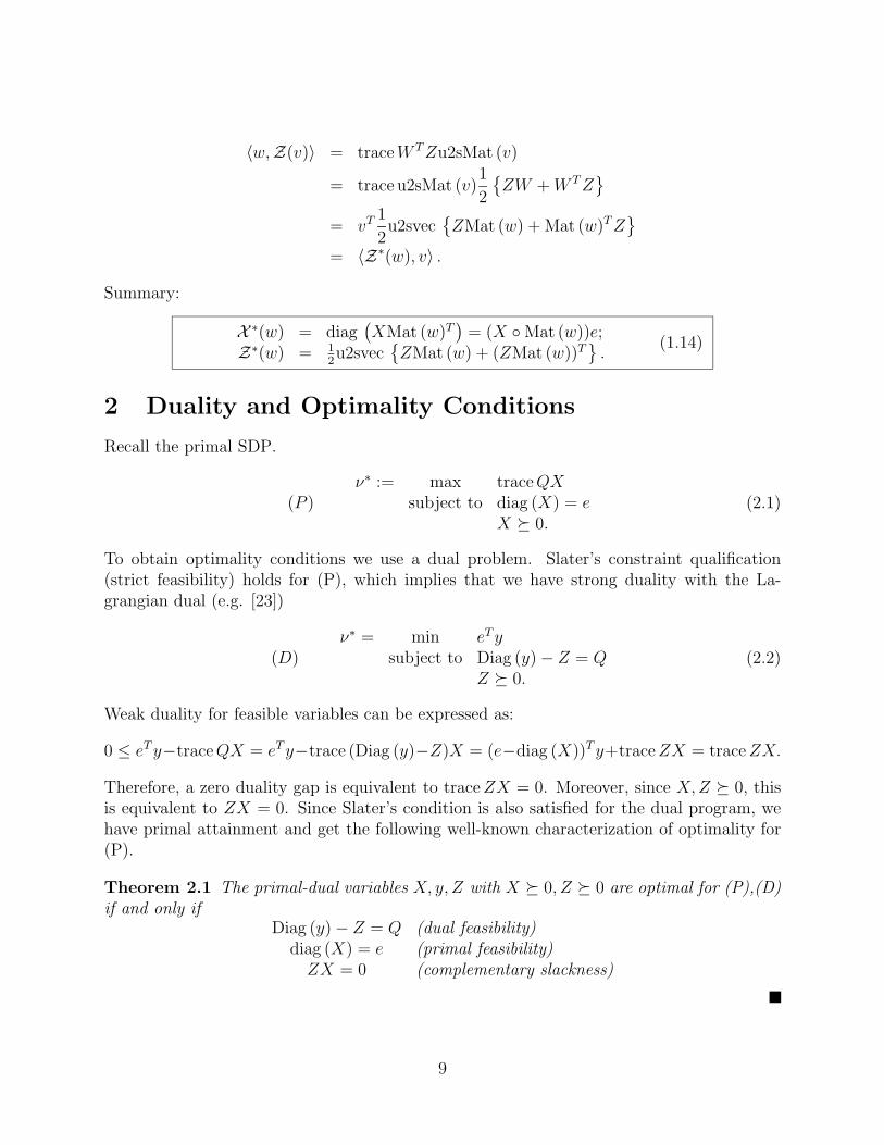
Summary:

X ∗(w) = diag(

XMat (w)T)

= (X ◦Mat (w))e;Z∗(w) = 1

2u2svec

{

ZMat (w) + (ZMat (w))T}

.(1.14)

2 Duality and Optimality Conditions

Recall the primal SDP.

(P )ν∗ := max trace QX

subject to diag (X) = eX � 0.

(2.1)

To obtain optimality conditions we use a dual problem. Slater’s constraint qualification(strict feasibility) holds for (P), which implies that we have strong duality with the La-grangian dual (e.g. [23])

(D)ν∗ = min eT y

subject to Diag (y)− Z = QZ � 0.

(2.2)

Weak duality for feasible variables can be expressed as:

0 ≤ eT y−trace QX = eT y−trace (Diag (y)−Z)X = (e−diag (X))T y+trace ZX = trace ZX.

Therefore, a zero duality gap is equivalent to trace ZX = 0. Moreover, since X, Z � 0, thisis equivalent to ZX = 0. Since Slater’s condition is also satisfied for the dual program, wehave primal attainment and get the following well-known characterization of optimality for(P).

Theorem 2.1 The primal-dual variables X, y, Z with X � 0, Z � 0 are optimal for (P),(D)if and only if

Diag (y)− Z = Q (dual feasibility)diag (X) = e (primal feasibility)

ZX = 0 (complementary slackness)

9

2.1 Preprocessing

Since the diagonal of X is fixed, we can use the constant K = eT diag (Q) in the objectivefunction. We could also set diag (Q) = 0 so that K = 0. Therefore we assume without lossof generality that

Diag (Q) = 0.

The simplicity of the primal feasibility equation yields an equivalent problem to (P) with therepresentation x = u2svec (X), X = u2sMat (x) + I. This representation is a key elementin our approach, i.e. we found an initial positive solution using an operator whose rangeis the null space of A . In the general SDP notation, we found AX = b is equivalent toX = N (x) + X, where N is a linear operator with range equal to the null space of A andX is a particular solution that satisfies X = N (x) + X ≻ 0. This approach can be directlyapplied to general problems with constraints of the form AX � b, X � 0. Obtaining aninitial feasible starting point can be done using the self-dual embedding e.g. [6, 7].

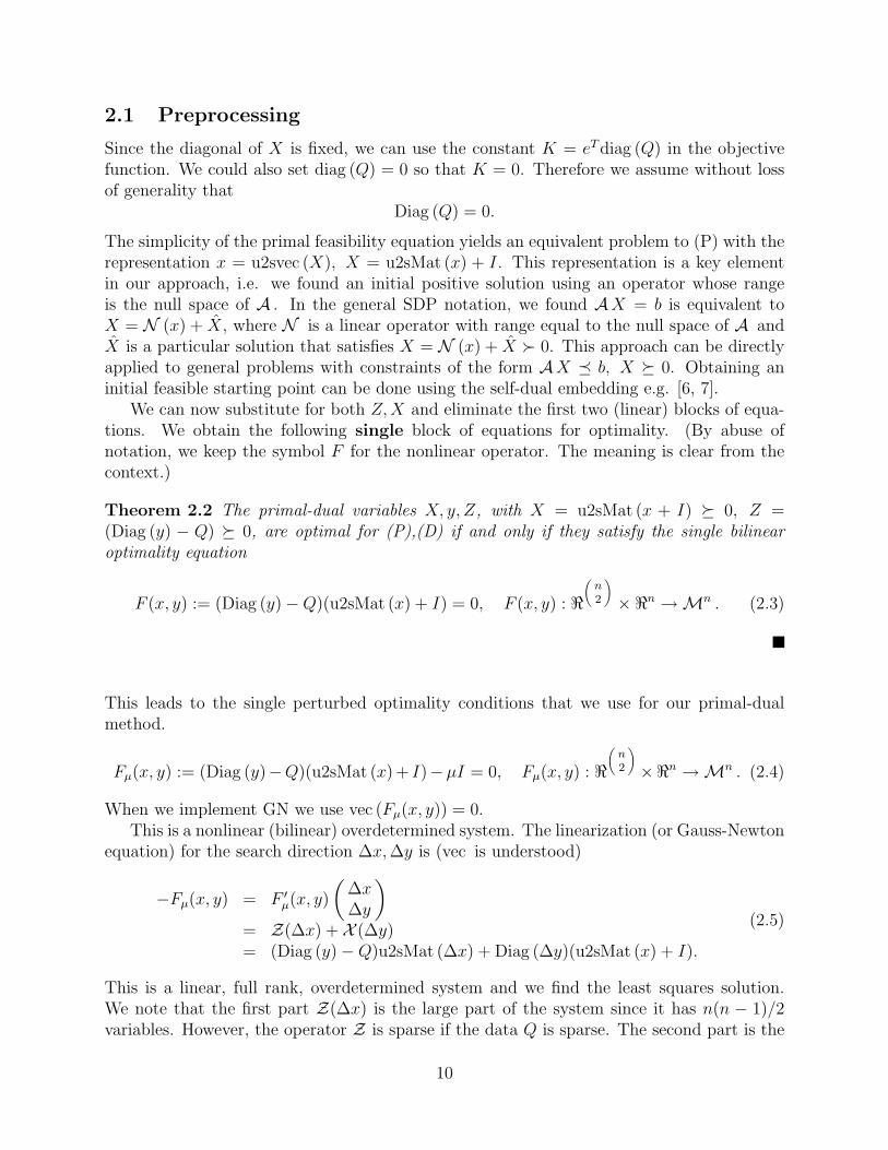
We can now substitute for both Z,X and eliminate the first two (linear) blocks of equa-tions. We obtain the following single block of equations for optimality. (By abuse ofnotation, we keep the symbol F for the nonlinear operator. The meaning is clear from thecontext.)

Theorem 2.2 The primal-dual variables X, y, Z, with X = u2sMat (x + I) � 0, Z =(Diag (y) − Q) � 0, are optimal for (P),(D) if and only if they satisfy the single bilinearoptimality equation

F (x, y) := (Diag (y)−Q)(u2sMat (x) + I) = 0, F (x, y) : ℜ(

n2

)

×ℜn →Mn . (2.3)

This leads to the single perturbed optimality conditions that we use for our primal-dualmethod.

Fµ(x, y) := (Diag (y)−Q)(u2sMat (x)+ I)−µI = 0, Fµ(x, y) : ℜ(

n2

)

×ℜn →Mn . (2.4)

When we implement GN we use vec (Fµ(x, y)) = 0.This is a nonlinear (bilinear) overdetermined system. The linearization (or Gauss-Newton

equation) for the search direction ∆x, ∆y is (vec is understood)

−Fµ(x, y) = F ′µ(x, y)

(

∆x∆y

)

= Z(∆x) + X (∆y)= (Diag (y)−Q)u2sMat (∆x) + Diag (∆y)(u2sMat (x) + I).

(2.5)

This is a linear, full rank, overdetermined system and we find the least squares solution.We note that the first part Z(∆x) is the large part of the system since it has n(n − 1)/2variables. However, the operator Z is sparse if the data Q is sparse. The second part is the

10

small part since it only has n variables, though the operator X is usually dense. This is thesize of the Schur complement system that arises in the standard approaches for SDP. Sparseleast squares techniques can be applied. In particular, the distinct division into two sets ofcolumns can be exploited using projection and multifrontal methods, e.g. [4, 14, 20, 21].

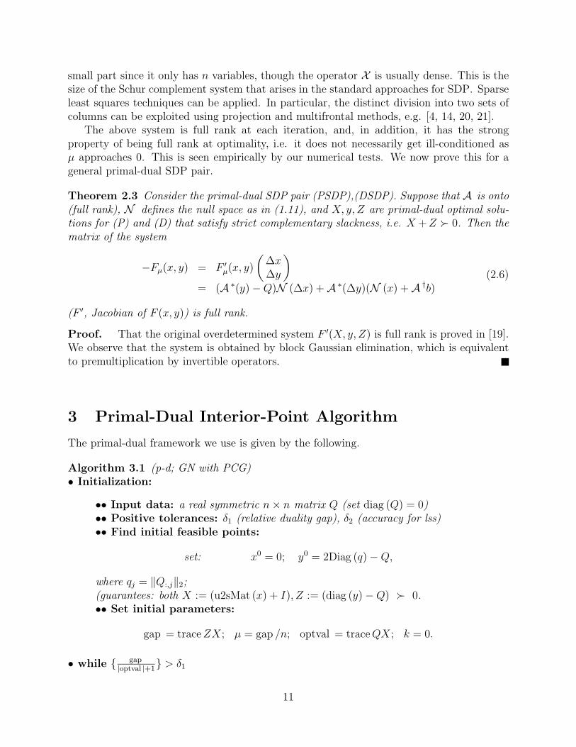
The above system is full rank at each iteration, and, in addition, it has the strongproperty of being full rank at optimality, i.e. it does not necessarily get ill-conditioned asµ approaches 0. This is seen empirically by our numerical tests. We now prove this for ageneral primal-dual SDP pair.

Theorem 2.3 Consider the primal-dual SDP pair (PSDP),(DSDP). Suppose that A is onto(full rank), N defines the null space as in (1.11), and X, y, Z are primal-dual optimal solu-tions for (P) and (D) that satisfy strict complementary slackness, i.e. X + Z ≻ 0. Then thematrix of the system

−Fµ(x, y) = F ′µ(x, y)

(

∆x∆y

)

= (A ∗(y)−Q)N (∆x) +A ∗(∆y)(N (x) +A †b)(2.6)

(F ′, Jacobian of F (x, y)) is full rank.

Proof. That the original overdetermined system F ′(X, y, Z) is full rank is proved in [19].We observe that the system is obtained by block Gaussian elimination, which is equivalentto premultiplication by invertible operators.

3 Primal-Dual Interior-Point Algorithm

The primal-dual framework we use is given by the following.

Algorithm 3.1 (p-d; GN with PCG)• Initialization:

•• Input data: a real symmetric n× n matrix Q (set diag (Q) = 0)•• Positive tolerances: δ1 (relative duality gap), δ2 (accuracy for lss)•• Find initial feasible points:

set: x0 = 0; y0 = 2Diag (q)−Q,

where qj = ‖Q:,j‖2;(guarantees: both X := (u2sMat (x) + I), Z := (diag (y)−Q) ≻ 0.•• Set initial parameters:

gap = trace ZX; µ = gap /n; optval = trace QX; k = 0.

• while { gap|optval |+1

} > δ1

11

•• solve for the search direction (to tolerance max

{

δ210

, min{µ1

3 ,1}106

}

, in a least

squares sense with PCG, using k-th iterate (x, y) = (xk, yk))

F ′σµ(x, y)

(

∆x∆y

)

= −Fσµ(x, y),

where σk centering, µk = trace (Diag (y)−Q)(u2sMat (x) + I)/n

xk+1 = x + αk∆x, yk+1 = y + αk∆y; αk > 0,

so that both (X := u2sMat (xk+1) + I), (Z := Diag (yk+1) − Q) ≻ 0, before thecrossover; so that sufficient decrease in ‖ZX‖F is guaranteed, after the crossover.•• update

k ← k + 1 and then update

µk, σk (σk = 0 after the crossover).

• end (while).• Conclusion: optimal X is approx. u2sMat (x) + I

We use equation (2.4) and the linearization (2.5) to develop the primal-dual interior-pointAlgorithm 3.1, (This modifies the standard approach in e.g. [28].) We include a centeringparameter σk (rather than the customary predictor-corrector approach). Our approach dif-fers in that we have eliminated, in advance, the primal and dual linear feasibility equations.We work with an overdetermined nonlinear system rather than a square symmetrized sys-tem; thus we use a Gauss-Newton approach, [19]. We use a crossover step, i.e. we use affinescaling, σ = 0, and we do not backtrack to preserve positive definiteness of Z,X once wehave found the region of quadratic convergence. The search direction is found using a pre-conditioned conjugate gradient method, lsqr [22]. The cost of each CG iteration is a (sparse)matrix multiplication and a diagonal matrix scaling, see e.g. (2.5).

There are many advantages for this algorithm:•Primal and dual feasibility is exact during each iteration (assuming that the the basis forthe null space was computed precisely);•there is no (costly, dense) Schur complement system to form;•There is no need to find Z−1 (which becomes ill-conditioned as µ goes to 0);•the sparsity of the data Q is exploited completely;•by the robustness of the algorithm, there is no need to enforce positivity of Z,X once µgets small enough; q-quadratic convergence is obtained;•the entire work of the algorithm lies in finding the search direction at each iteration bysolving a (sparse) least squares problem using a CG type algorithm. Each iteration of theCG algorithm involves a (sparse) matrix-matrix multiplication and a diagonal row scalingof a matrix. The more efficiently we can solve these least squares problems, the faster ouralgorithm will be. Better preconditioners, better solvers, and better parallelization in thefuture will improve the algorithm;•the techniques can be extended directly to general SDPs, depending on efficient (sparse)representations of the primal (and/or dual) feasibility equation.

12

3.1 Preconditioning

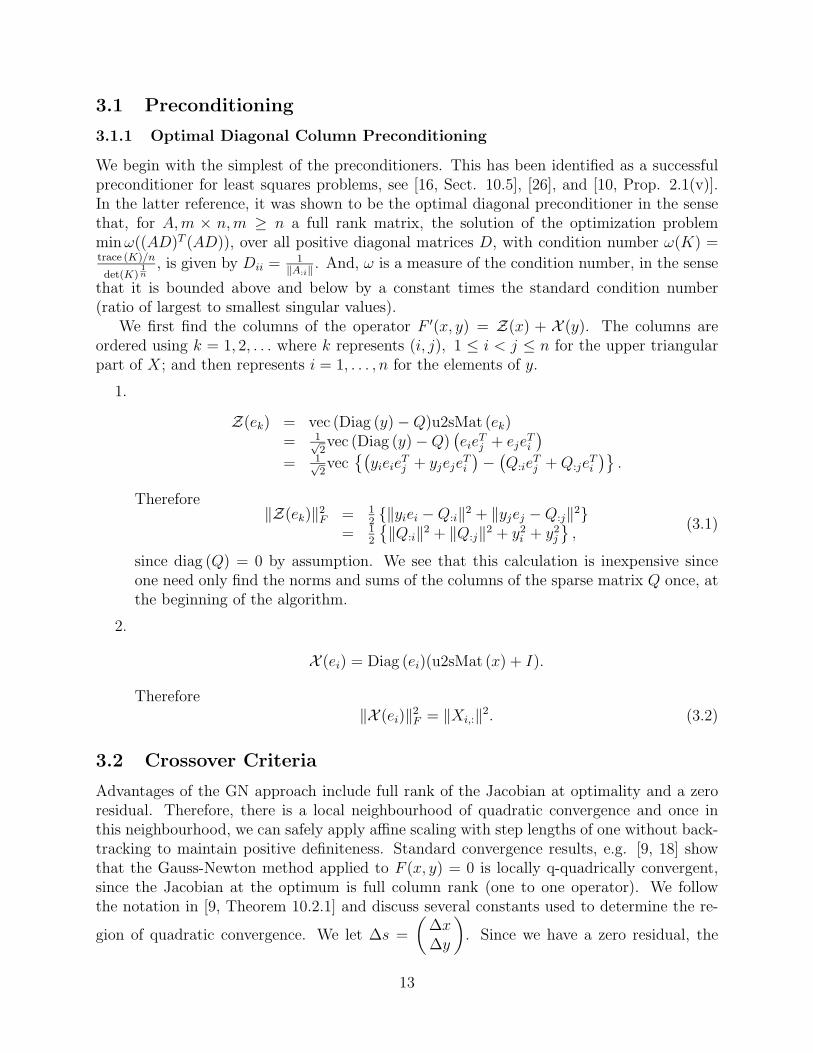
3.1.1 Optimal Diagonal Column Preconditioning

We begin with the simplest of the preconditioners. This has been identified as a successfulpreconditioner for least squares problems, see [16, Sect. 10.5], [26], and [10, Prop. 2.1(v)].In the latter reference, it was shown to be the optimal diagonal preconditioner in the sensethat, for A, m × n, m ≥ n a full rank matrix, the solution of the optimization problemmin ω((AD)T (AD)), over all positive diagonal matrices D, with condition number ω(K) =trace (K)/n

det(K)1n

, is given by Dii = 1‖A:i‖ . And, ω is a measure of the condition number, in the sense

that it is bounded above and below by a constant times the standard condition number(ratio of largest to smallest singular values).

We first find the columns of the operator F ′(x, y) = Z(x) + X (y). The columns areordered using k = 1, 2, . . . where k represents (i, j), 1 ≤ i < j ≤ n for the upper triangularpart of X; and then represents i = 1, . . . , n for the elements of y.

1.

Z(ek) = vec (Diag (y)−Q)u2sMat (ek)= 1√

2vec (Diag (y)−Q)

(

eieTj + eje

Ti

)

= 1√2vec

{(

yieieTj + yjeje

Ti

)

−(

Q:ieTj + Q:je

Ti

)}

.

Therefore‖Z(ek)‖2F = 1

2{‖yiei −Q:i‖2 + ‖yjej −Q:j‖2}

= 12

{

‖Q:i‖2 + ‖Q:j‖2 + y2i + y2

j

}

,(3.1)

since diag (Q) = 0 by assumption. We see that this calculation is inexpensive sinceone need only find the norms and sums of the columns of the sparse matrix Q once, atthe beginning of the algorithm.

2.

X (ei) = Diag (ei)(u2sMat (x) + I).

Therefore‖X (ei)‖2F = ‖Xi,:‖2. (3.2)

3.2 Crossover Criteria

Advantages of the GN approach include full rank of the Jacobian at optimality and a zeroresidual. Therefore, there is a local neighbourhood of quadratic convergence and once inthis neighbourhood, we can safely apply affine scaling with step lengths of one without back-tracking to maintain positive definiteness. Standard convergence results, e.g. [9, 18] showthat the Gauss-Newton method applied to F (x, y) = 0 is locally q-quadrically convergent,since the Jacobian at the optimum is full column rank (one to one operator). We followthe notation in [9, Theorem 10.2.1] and discuss several constants used to determine the re-

gion of quadratic convergence. We let ∆s =

(

∆x∆y

)

. Since we have a zero residual, the

13

corresponding constant σ = 0. Since

‖F ′(∆s)‖F = ‖Zu2sMat (∆x) + Diag (∆y)X‖F≤ ‖Zu2sMat (∆x)‖F + ‖Diag (∆y)X‖F≤ ‖Z‖F‖u2sMat (∆x)‖F + ‖Diag (∆y)‖F‖X‖F= ‖Z‖F‖∆x‖2 + ‖∆y‖2‖X‖F≤

√

‖Z‖2F + ‖X‖2F‖∆s‖2, (by Cauchy-Schwartz inequality)

the bound on the norm of the Jacobian is

α =√

‖Z‖2F + ‖X‖2F .

‖F ′(s− s)(∆s)‖F = ‖(Z − Z)u2sMat (∆x) + Diag (∆y)(X − X)‖F≤ ‖(Z − Z)‖F‖u2sMat (∆x)‖F + ‖Diag (∆y)‖F‖(X − X)‖F= ‖(y − y)‖2‖∆x‖2 + ‖∆y‖2‖(x− x)‖2.

Therefore the Lipschitz constant isγ = 1. (3.3)

Now suppose that the optimum s∗ is unique and the smallest singular value satisfiesσmin(F

′(s)) ≥√

K, for all s in an ǫ1 neighbourhood of s∗, for some constant K > 0.Following [9, Page 223], we define

ǫ := min

{

ǫ1,1

Kαγ

}

= min

{

ǫ1,1

K√

‖Z∗‖2F + ‖X∗‖2F

}

.

Then q-quadratic convergence is guaranteed once the current iterate is in this ǫ neigh-bourhood of the optimum. One possible heuristic for this is to start the crossover ifσmin(F

′(s)) ≥ 2‖ZX‖2. In our tests we started the crossover when the relative dualitygap trace ZX

|trace QX|+1< .1. This simpler heuristic never failed to converge, though q-quadratic

convergence was not immediately detected.

4 Numerical Tests

We have performed preliminary testing to illustrate some of the features of the method. Wesee that the crossover to using a steplength of 1, not maintaining interiority, and using affinescaling, has a significant effect on both the number of iterations and the conditioning of thelinear system. The number of iterations are approximately halved. The best results wereobtained by staying well-centered before the crossover. This is in line with what we knowfrom the theory. This appeared to help with the conditioning of the Jacobian and loweredthe number of CG iterations. For simplicity, the crossover was done when the relative dualitygap was less than .1 and we used a steplength of 1 after the crossover, rather than a linesearch to guarantee sufficient decrease in ‖ZX‖F . In all our tests on random problems, wenever failed to converge to a high accuracy solution.

The tests were done using MATLAB 6.0.0.88 (R12) on a SUNW, Ultra 5− 10 with oneGB of RAM using SunOS 5.8 (denoted by SUN), as well as on a Toshiba Pentium II, 300

14

MHZ, with 128 MB of RAM (denoted by PII). 99% of the cputime was spent on finding thesearch direction, i.e. in the PCG part of the code in finding the (approximate) least squaressolution of the Gauss-Newton equation. Randomly generated problems of size up to n = 550were solved in a reasonable time to high accuracy. To prevent zero columns in Q, the firstupper (lower) diagonal of Q was set to a vector of ones.

The cost for the early iterations was very low, e.g. 21, 50 CG iterations, 24, 58 cpu secondsfor the first two iterations for n = 365 on the SUN. This cost increased as the relative dualitygap (and the requested tolerance for the least squares solution) decreased. Low accuracysolutions were obtained quickly, e.g. one decimal accuracy after 4 to 5 iterations. The costper iteration increased steadily and then levelled off near the optimum.

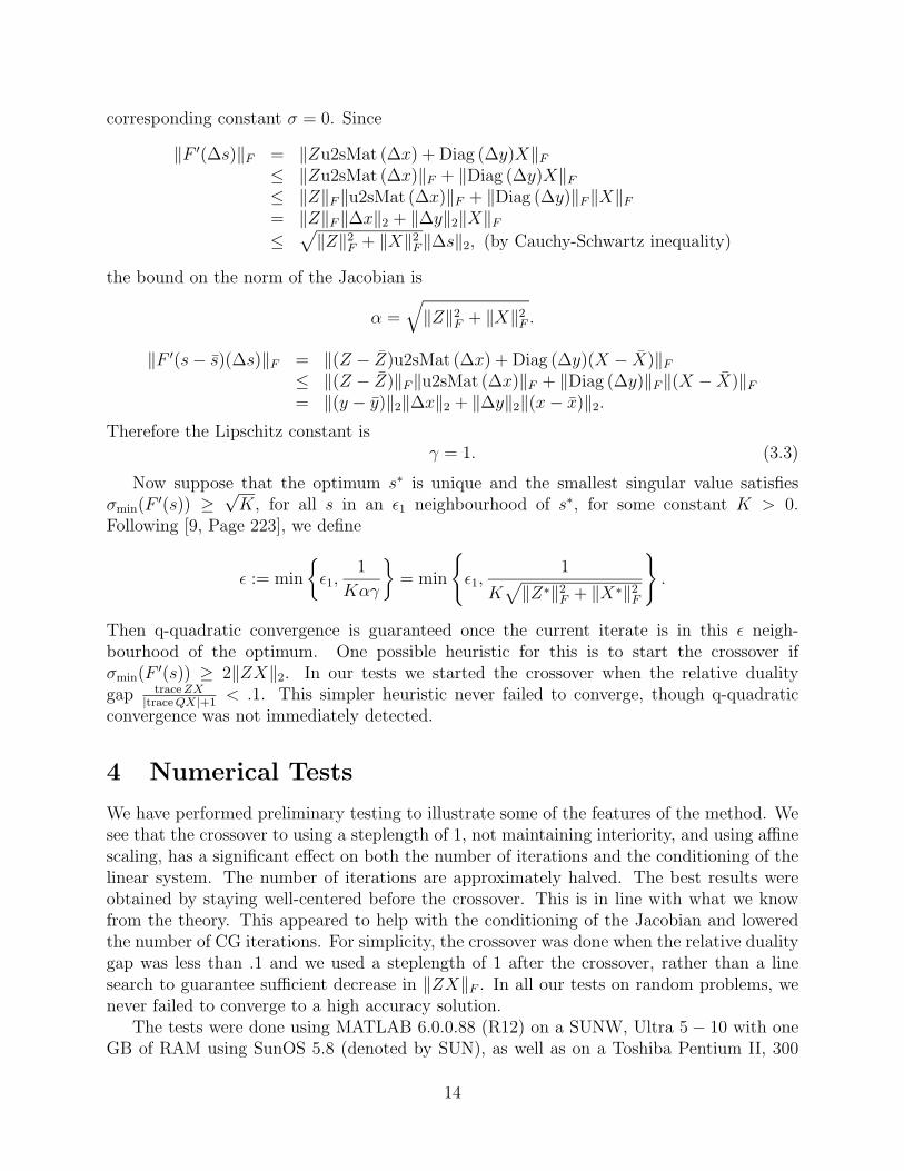
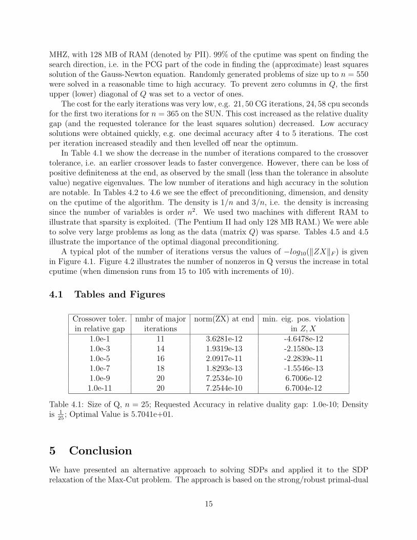
In Table 4.1 we show the decrease in the number of iterations compared to the crossovertolerance, i.e. an earlier crossover leads to faster convergence. However, there can be loss ofpositive definiteness at the end, as observed by the small (less than the tolerance in absolutevalue) negative eigenvalues. The low number of iterations and high accuracy in the solutionare notable. In Tables 4.2 to 4.6 we see the effect of preconditioning, dimension, and densityon the cputime of the algorithm. The density is 1/n and 3/n, i.e. the density is increasingsince the number of variables is order n2. We used two machines with different RAM toillustrate that sparsity is exploited. (The Pentium II had only 128 MB RAM.) We were ableto solve very large problems as long as the data (matrix Q) was sparse. Tables 4.5 and 4.5illustrate the importance of the optimal diagonal preconditioning.

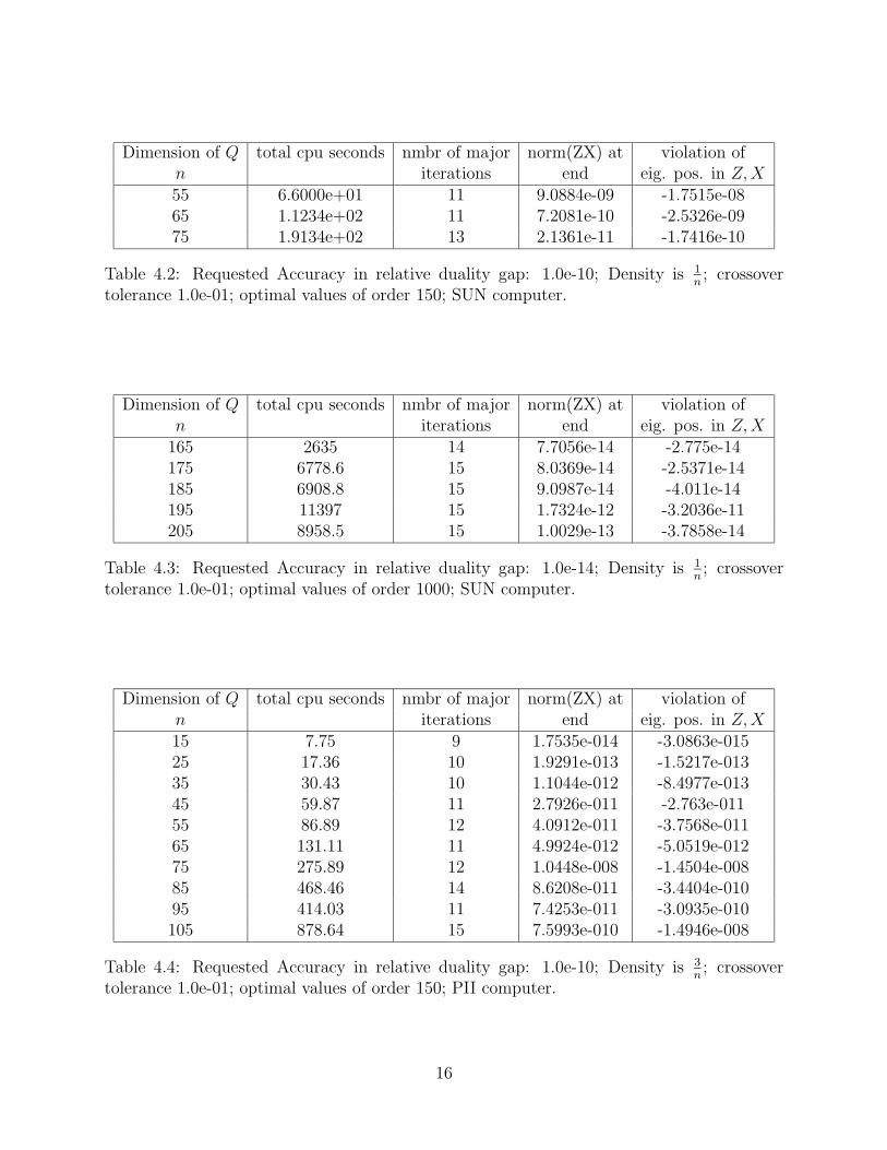
A typical plot of the number of iterations versus the values of −log10(‖ZX‖F ) is givenin Figure 4.1. Figure 4.2 illustrates the number of nonzeros in Q versus the increase in totalcputime (when dimension runs from 15 to 105 with increments of 10).

4.1 Tables and Figures

Crossover toler. nmbr of major norm(ZX) at end min. eig. pos. violationin relative gap iterations in Z,X

1.0e-1 11 3.6281e-12 -4.6478e-121.0e-3 14 1.9319e-13 -2.1580e-131.0e-5 16 2.0917e-11 -2.2839e-111.0e-7 18 1.8293e-13 -1.5546e-131.0e-9 20 7.2534e-10 6.7006e-121.0e-11 20 7.2544e-10 6.7004e-12

Table 4.1: Size of Q, n = 25; Requested Accuracy in relative duality gap: 1.0e-10; Densityis 1

25; Optimal Value is 5.7041e+01.

5 Conclusion

We have presented an alternative approach to solving SDPs and applied it to the SDPrelaxation of the Max-Cut problem. The approach is based on the strong/robust primal-dual

15

Dimension of Q total cpu seconds nmbr of major norm(ZX) at violation ofn iterations end eig. pos. in Z,X55 6.6000e+01 11 9.0884e-09 -1.7515e-0865 1.1234e+02 11 7.2081e-10 -2.5326e-0975 1.9134e+02 13 2.1361e-11 -1.7416e-10

Table 4.2: Requested Accuracy in relative duality gap: 1.0e-10; Density is 1n; crossover

tolerance 1.0e-01; optimal values of order 150; SUN computer.

Dimension of Q total cpu seconds nmbr of major norm(ZX) at violation ofn iterations end eig. pos. in Z,X

165 2635 14 7.7056e-14 -2.775e-14175 6778.6 15 8.0369e-14 -2.5371e-14185 6908.8 15 9.0987e-14 -4.011e-14195 11397 15 1.7324e-12 -3.2036e-11205 8958.5 15 1.0029e-13 -3.7858e-14

Table 4.3: Requested Accuracy in relative duality gap: 1.0e-14; Density is 1n; crossover

tolerance 1.0e-01; optimal values of order 1000; SUN computer.

Dimension of Q total cpu seconds nmbr of major norm(ZX) at violation ofn iterations end eig. pos. in Z,X15 7.75 9 1.7535e-014 -3.0863e-01525 17.36 10 1.9291e-013 -1.5217e-01335 30.43 10 1.1044e-012 -8.4977e-01345 59.87 11 2.7926e-011 -2.763e-01155 86.89 12 4.0912e-011 -3.7568e-01165 131.11 11 4.9924e-012 -5.0519e-01275 275.89 12 1.0448e-008 -1.4504e-00885 468.46 14 8.6208e-011 -3.4404e-01095 414.03 11 7.4253e-011 -3.0935e-010105 878.64 15 7.5993e-010 -1.4946e-008

Table 4.4: Requested Accuracy in relative duality gap: 1.0e-10; Density is 3n; crossover

tolerance 1.0e-01; optimal values of order 150; PII computer.

16

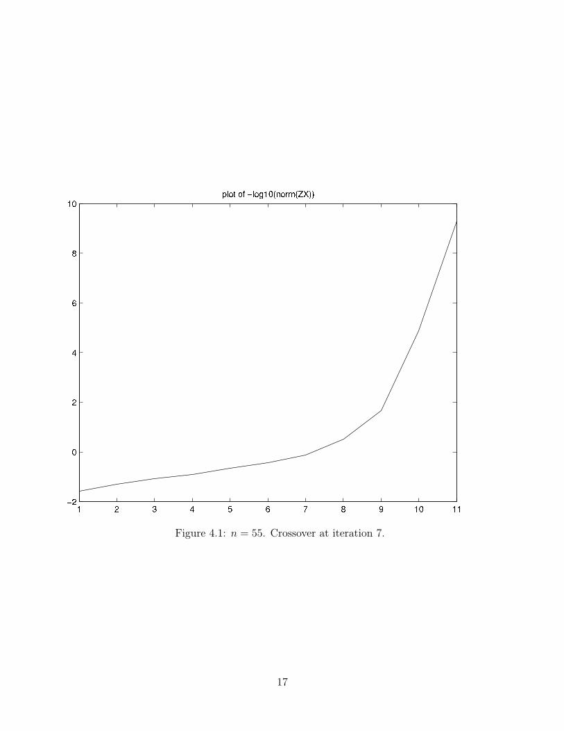
Figure 4.1: n = 55. Crossover at iteration 7.

17

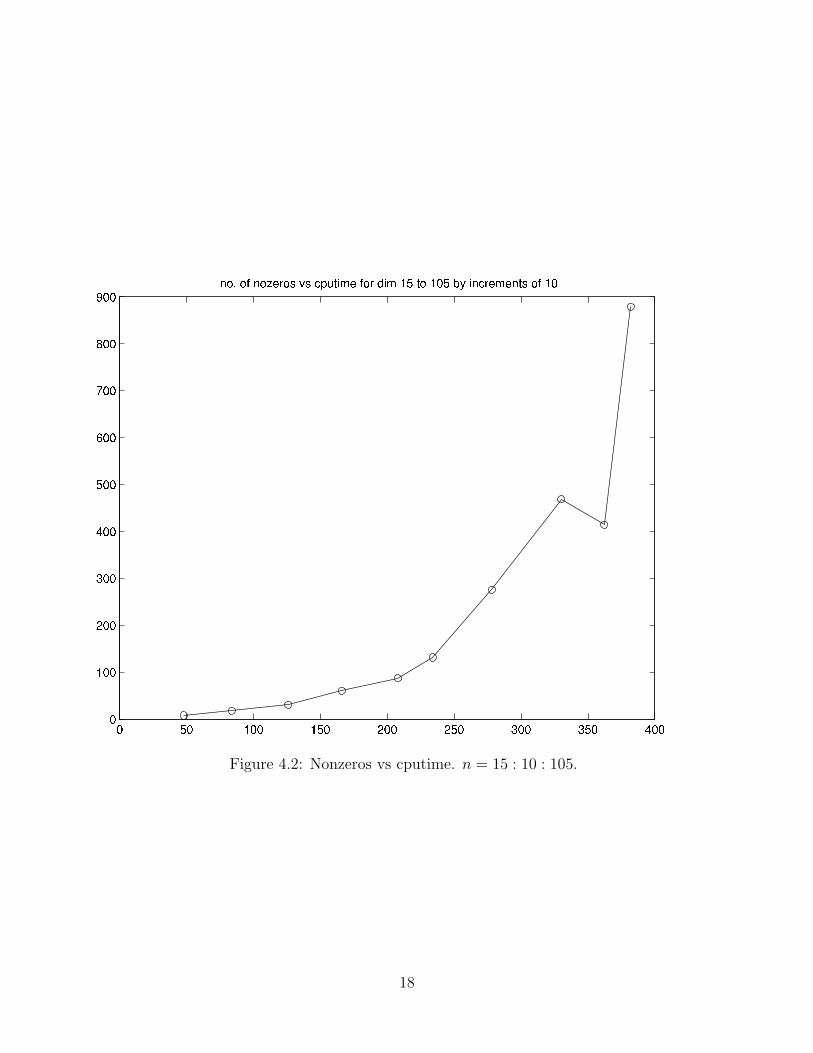
Figure 4.2: Nonzeros vs cputime. n = 15 : 10 : 105.

18

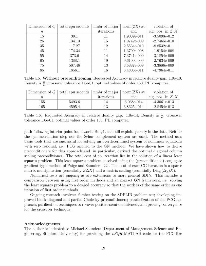
Dimension of Q total cpu seconds nmbr of major norm(ZX) at violation ofn iterations end eig. pos. in Z,X15 30.1 11 1.9039e-011 -3.5098e-01225 134.13 15 1.9742e-009 -2.7465e-01035 117.27 12 2.5534e-010 -8.8532e-01145 174.34 11 1.3799e-008 -1.9154e-00855 373.6 14 7.3741e-009 -3.1854e-00965 1388.1 19 9.6109e-009 -2.7634e-00975 507.46 13 3.5887e-009 -3.3886e-00985 1856.1 16 6.4806e-011 -4.7964e-011

Table 4.5: Without preconditioning; Requested Accuracy in relative duality gap: 1.0e-10;Density is 3

n; crossover tolerance 1.0e-01; optimal values of order 150; PII computer.

Dimension of Q total cpu seconds nmbr of major norm(ZX) at violation ofn iterations end eig. pos. in Z,X

155 5493.6 14 6.068e-014 -4.3061e-013165 4595.4 13 3.8625e-014 -2.8454e-013

Table 4.6: Requested Accuracy in relative duality gap: 1.0e-14; Density is 1n; crossover

tolerance 1.0e-01; optimal values of order 150; PII computer.

path-following interior-point framework. But, it can still exploit sparsity in the data. Neitherthe symmetrization step nor the Schur complement system are used. The method usesbasic tools that are successful for solving an overdetermined system of nonlinear equationswith zero residual, i.e. PCG applied to the GN method. We have shown how to derivepreconditioners for this approach and, in particular, derived the optimal diagonal columnscaling preconditioner. The total cost of an iteration lies in the solution of a linear leastsquares problem. This least squares problem is solved using the (preconditioned) conjugategradient type method of Paige and Saunders [22]. The cost of each CG iteration is a sparsematrix multiplication (essentially Z∆X) and a matrix scaling (essentially Diag (∆y)X).

Numerical tests are ongoing as are extensions to more general SDPs. This includes acomparison between using first order methods and an inexact GN framework, i.e. solvingthe least squares problem to a desired accuracy so that the work is of the same order as oneiteration of first order methods.

Ongoing research involves: further testing on the SDPLIB problem set; developing im-proved block diagonal and partial Cholesky preconditioners; parallelization of the PCG ap-proach; purification techniques to recover positive semi-definiteness; and proving convergencefor the crossover technique.

AcknowledgmentsThe author is indebted to Michael Saunders (Department of Management Science and En-gineering, Stanford University) for providing the LSQR MATLAB code for the PCG-like

19

method. The author would also like to thank Nick Higham (Department of Mathematics,University of Manchester) and Levent Tuncel (Department of Combinatorics and Optimiza-tion, Univerity of Waterloo) for many helpful discussions and comments.

References

[1] M.F. ANJOS, N. HIGHAM, and H. WOLKOWICZ. A semidefinite programming ap-proach for the closest correlation matrix problem. Technical Report CORR 2001-inprogress, University of Waterloo, Waterloo, Ontario, 2001.

[2] M.F. ANJOS and H. WOLKOWICZ. A strengthened SDP relaxation via a secondlifting for the Max-Cut problem. Special Issue of Discrete Applied Mathematics devotedto Foundations of Heuristics in Combinatorial Optimization, to appear.

[3] S. J. BENSON, Y. YE, and X. ZHANG. Solving large-scale sparse semidefinite programsfor combinatorial optimization. SIAM J. Optim., 10(2):443–461 (electronic), 2000.

[4] A. BJORCK. Methods for sparse least squares problems. In J.R. Bunch and D. J. Rose,editors, Sparse Matrix Computations, pages 177–199. Academic Press, New York, 1976.

[5] S. BURER and R.D.C. MONTEIRO. A projected gradient algorithm for solving themaxcut SDP relaxation. Optimization Methods and Software, 15(3-4):175–200, 2001.

[6] E. de KLERK. Interior point methods for semidefinite programming. PhD thesis, DelftUniversity, 1997.

[7] E. de KLERK, C. ROOS, and T. TERLAKY. Initialization in semidefinite programmingvia a self-dual skew-symmetric embedding. Oper. Res. Lett., 20(5):213–221, 1997.

[8] R.S DEMBO, S.C. EISENSTAT, and T. STEIHAUG. Inexact Newton methods. SIAMJ. Numer. Anal., 19:400–408, 1982.

[9] J.E. DENNIS Jr. and R.B. SCHNABEL. Numerical methods for unconstrained optimiza-tion and nonlinear equations, volume 16 of Classics in Applied Mathematics. Societyfor Industrial and Applied Mathematics (SIAM), Philadelphia, PA, 1996. Correctedreprint of the 1983 original.

[10] J.E. DENNIS Jr. and H. WOLKOWICZ. Sizing and least-change secant methods. SIAMJ. Numer. Anal., 30(5):1291–1314, 1993.

[11] M.M. DEZA and M. LAURENT. Geometry of cuts and metrics. Springer-Verlag, Berlin,1997.

[12] A.V. FIACCO and G.P. McCORMICK. Nonlinear programming. Society for Industrialand Applied Mathematics (SIAM), Philadelphia, PA, second (first 1968) edition, 1990.Sequential unconstrained minimization techniques.

20

[13] M.X. GOEMANS and F. RENDL. Combinatorial optimization. In H. Wolkowicz, R. Sai-gal, and L. Vandenberghe, editors, HANDBOOK OF SEMIDEFINITE PROGRAM-MING: Theory, Algorithms, and Applications. Kluwer Academic Publishers, Boston,MA, 2000.

[14] G. H. GOLUB and V. PEREYRA. The differentiation of pseudoinverses and nonlinearleast squares problems whose variables separate. SIAM J. Numer. Anal., 10:413–432,1973.

[15] M. GONZALEZ-LIMA and H. WOLKOWICZ. Primal-dual methods using least squaresfor linear programming. Technical Report CORR 2001-in progress, University of Wa-terloo, Waterloo, Ontario, 2001.

[16] A. GREENBAUM. Iterative methods for solving linear systems. Society for Industrialand Applied Mathematics (SIAM), Philadelphia, PA, 1997.

[17] C. HELMBERG and F. RENDL. A spectral bundle method for semidefinite program-ming. SIAM J. Optim., 10(3):673 – 696, 2000.

[18] C. T. KELLEY. Iterative methods for linear and nonlinear equations. Society forIndustrial and Applied Mathematics (SIAM), Philadelphia, PA, 1995. With separatelyavailable software.

[19] S. KRUK, M. MURAMATSU, F. RENDL, R.J. VANDERBEI, and H. WOLKOWICZ.The Gauss-Newton direction in linear and semidefinite programming. OptimizationMethods and Software, 15(1):1–27, 2001.

[20] P. MATSTOMS. The Multifrontal Solution of Sparse Linear Least Squares Problems.Licentiat thesis, Department of Mathematics, Linkoping University, Sweden, 1991.

[21] P. MATSTOMS. Sparse QR factorization in MATLAB. ACM Trans. Math. Software,20:136–159, 1994.

[22] C.C. PAIGE and M.A. SAUNDERS. LSQR: an algorithm for sparse linear equationsand sparse least squares. ACM Trans. Math. Software, 8(1):43–71, 1982.

[23] M.V. RAMANA, L. TUNCEL, and H. WOLKOWICZ. Strong duality for semidefiniteprogramming. SIAM J. Optim., 7(3):641–662, 1997.

[24] F. RENDL, R. SOTIROV, and H. WOLKOWICZ. Exploiting sparsity in interior pointmethods: applications to SDP and QAP. Technical Report in progress, University ofWaterloo, Waterloo, Canada, 2001.

[25] M.J. TODD. A study of search directions in primal-dual interior-point methods forsemidefinite programming. Optim. Methods Softw., 11&12:1–46, 1999.

[26] A. VAN der SLUIS. Condition numbers and equilibration of matrices. Numer. Math.,14:14–23, 1969/1970.

21

[27] H. WOLKOWICZ, R. SAIGAL, and L. VANDENBERGHE, editors. HANDBOOK OFSEMIDEFINITE PROGRAMMING: Theory, Algorithms, and Applications. KluwerAcademic Publishers, Boston, MA, 2000. xxvi+654 pages.

[28] S. WRIGHT. Primal-Dual Interior-Point Methods. Society for Industrial and AppliedMathematics (SIAM), Philadelphia, Pa, 1996.

22

A Current Numerical Results

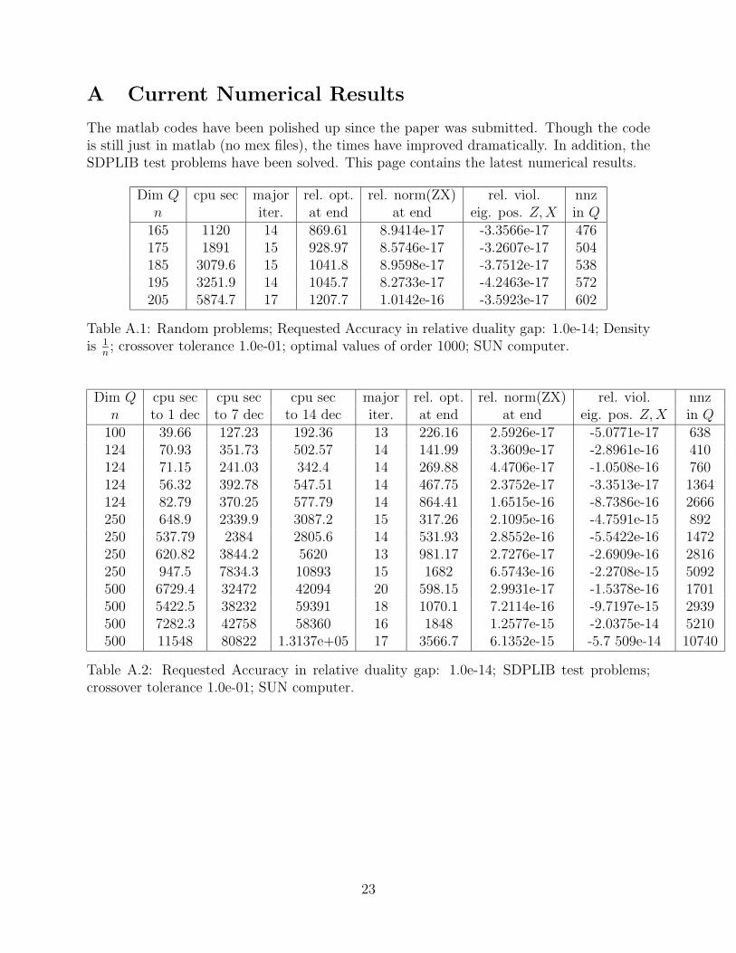
The matlab codes have been polished up since the paper was submitted. Though the codeis still just in matlab (no mex files), the times have improved dramatically. In addition, theSDPLIB test problems have been solved. This page contains the latest numerical results.

Dim Q cpu sec major rel. opt. rel. norm(ZX) rel. viol. nnzn iter. at end at end eig. pos. Z,X in Q

165 1120 14 869.61 8.9414e-17 -3.3566e-17 476175 1891 15 928.97 8.5746e-17 -3.2607e-17 504185 3079.6 15 1041.8 8.9598e-17 -3.7512e-17 538195 3251.9 14 1045.7 8.2733e-17 -4.2463e-17 572205 5874.7 17 1207.7 1.0142e-16 -3.5923e-17 602

Table A.1: Random problems; Requested Accuracy in relative duality gap: 1.0e-14; Densityis 1

n; crossover tolerance 1.0e-01; optimal values of order 1000; SUN computer.

Dim Q cpu sec cpu sec cpu sec major rel. opt. rel. norm(ZX) rel. viol. nnzn to 1 dec to 7 dec to 14 dec iter. at end at end eig. pos. Z,X in Q

100 39.66 127.23 192.36 13 226.16 2.5926e-17 -5.0771e-17 638124 70.93 351.73 502.57 14 141.99 3.3609e-17 -2.8961e-16 410124 71.15 241.03 342.4 14 269.88 4.4706e-17 -1.0508e-16 760124 56.32 392.78 547.51 14 467.75 2.3752e-17 -3.3513e-17 1364124 82.79 370.25 577.79 14 864.41 1.6515e-16 -8.7386e-16 2666250 648.9 2339.9 3087.2 15 317.26 2.1095e-16 -4.7591e-15 892250 537.79 2384 2805.6 14 531.93 2.8552e-16 -5.5422e-16 1472250 620.82 3844.2 5620 13 981.17 2.7276e-17 -2.6909e-16 2816250 947.5 7834.3 10893 15 1682 6.5743e-16 -2.2708e-15 5092500 6729.4 32472 42094 20 598.15 2.9931e-17 -1.5378e-16 1701500 5422.5 38232 59391 18 1070.1 7.2114e-16 -9.7197e-15 2939500 7282.3 42758 58360 16 1848 1.2577e-15 -2.0375e-14 5210500 11548 80822 1.3137e+05 17 3566.7 6.1352e-15 -5.7 509e-14 10740

Table A.2: Requested Accuracy in relative duality gap: 1.0e-14; SDPLIB test problems;crossover tolerance 1.0e-01; SUN computer.

23

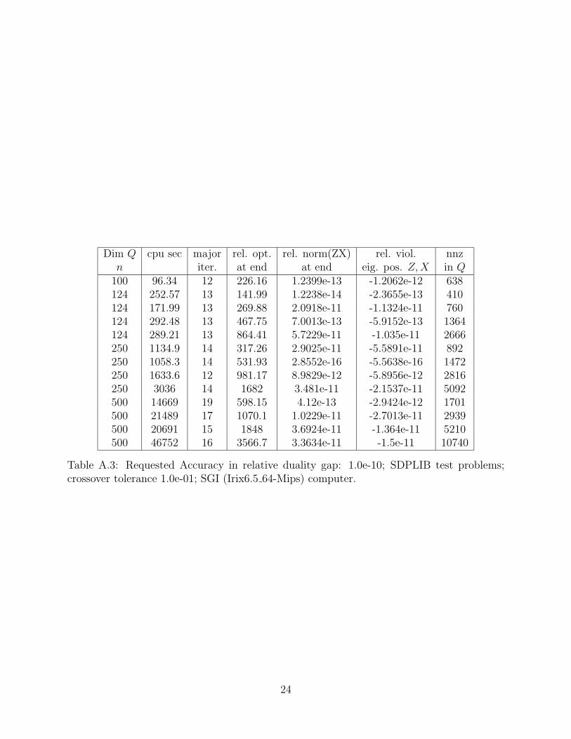
Dim Q cpu sec major rel. opt. rel. norm(ZX) rel. viol. nnzn iter. at end at end eig. pos. Z,X in Q

100 96.34 12 226.16 1.2399e-13 -1.2062e-12 638124 252.57 13 141.99 1.2238e-14 -2.3655e-13 410124 171.99 13 269.88 2.0918e-11 -1.1324e-11 760124 292.48 13 467.75 7.0013e-13 -5.9152e-13 1364124 289.21 13 864.41 5.7229e-11 -1.035e-11 2666250 1134.9 14 317.26 2.9025e-11 -5.5891e-11 892250 1058.3 14 531.93 2.8552e-16 -5.5638e-16 1472250 1633.6 12 981.17 8.9829e-12 -5.8956e-12 2816250 3036 14 1682 3.481e-11 -2.1537e-11 5092500 14669 19 598.15 4.12e-13 -2.9424e-12 1701500 21489 17 1070.1 1.0229e-11 -2.7013e-11 2939500 20691 15 1848 3.6924e-11 -1.364e-11 5210500 46752 16 3566.7 3.3634e-11 -1.5e-11 10740

Table A.3: Requested Accuracy in relative duality gap: 1.0e-10; SDPLIB test problems;crossover tolerance 1.0e-01; SGI (Irix6.5 64-Mips) computer.

24