SIMPLE DATA ANALYSISFOR BIOLOGISTS

ERIC BARANFIONA WARRY

SIMPLE DATA ANALYSISFOR BIOLOGISTS

Eric BARAN, Fiona WARRY

WorldFish Center is one of the 15 international researchcenters of the Consultative Group on InternationalAgricultural Research (CGIAR) that has initiated the publicawareness campaign, Future Harvest.

SIMPLE DATA ANALYSIS FOR BIOLOGISTS

Authors:Eric BARAN, Fiona WARRY

Published by the WorldFish Center and the Fisheries AdministrationHeadquarters: P.O. Box 500 GPO, 10670, Penang, MalaysiaGreater Mekong office: P.O. Box 1135 (Wat Phnom),

#35, Street 71, Sangkat Boeng Keng Kang 1Phnom Penh, CambodiaE-mail: worldfish-cambodia@cgiar.org

Citation: Baran E., Warry F. 2008 Simple data analysis for biologists. WorldFish Center and the FisheriesAdministration. Phnom Penh, Cambodia. 67 pages.

Photos by Paul Stewart | www.mouthtosource.netLayout and printing by Digital Graphic, Phnom Penh, CambodiaISBN: 9789995071011WorldFish Center Contribution No. 1881

AcknowledgmentsThis document was originally developed as lecture notes for hydrobiologists of the World HealthOrganization's Onchocerciasis Control Program in West Africa. Notes were substantially expandedduring the WorldFish/ADB project "Capacity building of the Inland Fisheries Research andDevelopment Institute" in Cambodia. Feedback and demand from trainees contributed to reshapingthe notes in order to better meet the needs of young fish biologists working in tropical countries. Thiswas the main impetus for developing an additional section on statistical tests and highlights thediffuse but essential contribution of multiple members of the Cambodian Fisheries Administration tothis document. This input was supplemented by that of trainees from Cantho University (Vietnam)in 2006, 2007, and 2008.

In this manual, the section on multivariate statistics is rooted in the Laboratory of Biometry andEvolutionary Biology of University Lyon 1 in France (http://pbil.univ lyon1.fr), and credit is due to Dr.Daniel Chessel and his colleagues of the French school of multivariate statistics for environmentaldata analysis for making complex methods accessible to a wide audience.

The section on statistical tests written by Fiona Warry was initially drafted by Ghislain Morard ofEcole Centrale in Paris. The Australian Youth Ambassadors for Development program in Cambodia,funded by AusAid, has contributed to this primer by funding the stay of Mrs. Warry during a year atWorldFish and at IFReDI.

Last, the creation of this document was financially supported by the European Commission and byWorldFish core funds.

The authors would like to express their sincere thanks to all these contributors.

TABLE OF CONTENTS

1. PRINCIPLES AND METHODS 61-1. MAIN FIELDS IN DATA ANALYSIS 61-2. TRANSLATING BIOLOGY INTO STATISTICS 8

1-2-1. Formulating a biological question 81-2-2. Terminology 91-2-3. Description of data acquired 91-2-4. Coding and formatting data 121-2-5. Translating biological questions into statistical questions 131-2-6. Amount of data required 131-2-7. Missing data 15

2. USING MS EXCEL FOR DATA ANALYSIS 162-1. MENU CUSTOMIZATION 162-2. SORTING DATA 182-3. FILTERING 182-4. USEFUL FORMULAS 192-5. PIVOT TABLE 202-6. CHARTS 23

2-6-1. Lines 232-6-2. Complex charts 242-6-3. Regression and trendlines 242-6-4. Charts with bars 242-6-5. Three dimensional charts 262-6-6. Customizing a chart 27

3. UNDERSTANDING EXPLORATORY ANALYSIS OF DATA 303-1. GEOMETRICAL APPROACH TO VARIABLES 31

3-1-1. Variables as dimensions 313-1-2. From variables to hyperspace 323-1-3. Variance as a geometric notion 33

3-2. OBJECTIVES AND PRINCIPLES OF MULTIVARIATE ANALYSIS 333-2-1. Projection onto a factorial map 333-2-2. Projection onto successive factorial maps 353-2-3. Projection of variables or of samples 35

3-3. SOME PROPERTIES OF MULTIVARIATE ANALYSES 363-4. READING A FACTORIAL MAP 37

3-4-1. Variables and repetitions 373-4-2. Map of variables, map of repetitions 373-4-3. Application 38

3-5. PRE-ANALYSIS DATA PROCESSING 403-5-1. Centering 403-5-2. Reducing 403-5-3. Normalizing 41

3-6. MAIN TYPES OF ANALYSES 413-6-1. One-table analyses (PCA, COA and others) 413-6-2. Two-table and K-table analyses 43

4. STASTICAL TESTS FOR COMPARING SAMPLES 464-1. DEFINITIONS AND PRINCIPLES 46

4-1-1. Mean, median, radiance 464-1-2. Normal distribution 474-1-3. Questions and hypotheses 484-1-4. Probability and significance 48

4-2. CHOOSING THE APPROPRIATE STATISTICAL TEST 494-2-1. Parametric versus non-parametric statistical tests 504-2-2. Transformations 504-2-3. Independent versus matched pairs 51

4-3. FROM EXCEL INTO SPSS 514-4. COMMON PARAMETRIC TESTS 52

4-4-1. Testing for normality and homogeneity of variances 524-4-2. T-test (Student's t-test) 544-4-3. Paired t-test 574-4-4. Simple Analyses of Variance (ANOVA) 59

4-5. SOME USEFUL NON-PARAMETRIC TESTS 614-5-1. Mann - Whitney U test 614-5-2. Wilcoxon test for matched pairs 634-5-3. Kruskal-Wallis test 64

This document is not just another course in statistics (lots of good books are available on themarket), but rather a simple introduction to research methods and analysis tools for biologists orenvironmental scientists, with particular emphasis on fish biology in developing countries.

Our initial assumptions, based on experience, are that the biologist has gathered data to answerbio-ecological questions, but he/she doesn't know anything about statistics, or has some vaguememories of arid formulas. He/she has access to a number of programs in statistical packages, butcould not find a simple book detailing the range of statistical methods or tools available. He/sheneeds numerical analyses and tests, but biology and statistics speak two different languages:ecological features and biological questions must be translated into quantitative tables andstatistical questions before they can be processed.

This primer therefore aims at reviewing some principles and tools, so that the biologist can:- ask questions and format data in a way compatible with numerical analysis;- explore data and perform basic analyses;- answer the questions he/she faces;- deepen knowledge in statistics books, without being repulsed straight away.

This document is thus divided into four main sections:-Principles and methods in data analysis (to pave the way for statistical analysis),-Simple - but effective - data processing with MS Excel,-Intuitive approach of multivariate analysises (an attempt to make these powerful methods more accessible), and

-Statistical tests for comparing samples, since this is one of the comon tasks in analysing data.

We hope that this manual will be useful to biologists, and will demonstrate that quality researchcan be achieved with simple and rigorous methods.

The authors

FOREWORD

Sim

ple

dat

a an

alys

is fo

r b

iolo

gis

ts

5

1-1. MAIN FIELDS IN DATA ANALYSIS

Two major fields exist in data analysis: exploratory methods and inferential statistics.

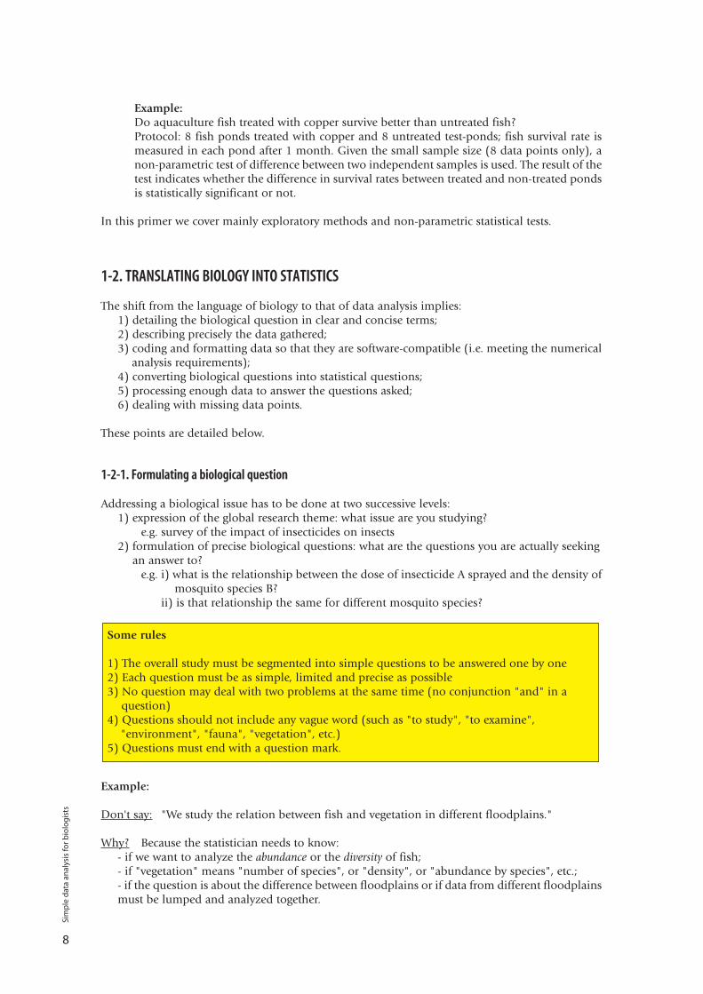
Exploratory analyses are also called "descriptive analyses". Their objectives are to:- simplify and clarify a situation or pattern not well known and apparently complex;- summarize the information contained in the data;- make apparent the relationships between variables.

Their way of expression is mostly graphic: histograms, scatter plots, factorial maps, etc. Thusexploratory statistics describe patterns or typologies. They do not assume any distribution amongvariables and they do not allow numerical testing of hypotheses.

Examples:

i) What is the relationship between fish migrations in ariver at certain times of the year, and the water level in thatriver at the same time? simple dual-axis histogram of fishcatches and water levels in the river

ii) what is the relationship between fish food regime, fishgrowth, maximal length and meat quality? factorial mapbased on a multivariate analysis; it highlights the relation-ship (= correlation) between herbivory and high growthrate, and the high meat quality of carnivore fishes.

1PRINCIPLES ANDMETHODS

6

Sim

ple

dat

a an

alys

is fo

r b

iolo

gis

ts

0

500

1000

1500

2000

0

2

4

6

8

10

12

14

Fish catchWater level

Wat

er le

vel i

n th

e riv

er (m

eter

s)

Fish

cat

ch (t

onne

s)

0

500

1000

1500

2000

0

2

4

6

8

10

12

14

Fish catchWater level

Wat

er le

vel i

n th

e riv

er (m

eter

s)

Fish

cat

ch (t

onne

s)

HerbivoresGrowth

Detritivores

CarnivoreMax length

Meat quality

HerbivoresGrowth

Detritivores

CarnivoreMax length

Meat quality

Inferential analyses, on the contrary, aim at predicting rules based on existing data, i.e. to inferfrom the sample to the population. Generally speaking inferential methods consist in quantifyinga dependent variable as a function of driving variables.

Example:Does the survival rate S of fish in an aquaculture pond depend upon (= is a function of)stocking density D? Protocol: 40 fish ponds with different stocking densities are monitored and the survival rateof fish in each pond is recorded. The relationship between S and D is calculated by a linearregression: Survival rate = f(stocking density) + errorOnce this equation is calculated, it allows predicting (= inferring) the survival rate of fishgiven the stocking density in any new pond.

Statistical tests are complementary tools often used to assess difference or similarity betweensamples.

Parametric tests are used for data that follow a standard distribution (e.g. normal,binomial, hypergeometric, etc.), and use the parameters of that distribution, such as averageor standard deviation. They require a fairly high sample size (see section 4).Non parametric tests, on the contrary, do not assume any distribution in data but are lesspowerful than parametric tests in detecting differences; however they are often useful tobiologists since they require much less data than parametric tests.

7

Sim

ple

dat

a an

alys

is fo

r b

iolo

gis

ts

8

Example:Do aquaculture fish treated with copper survive better than untreated fish?Protocol: 8 fish ponds treated with copper and 8 untreated test-ponds; fish survival rate ismeasured in each pond after 1 month. Given the small sample size (8 data points only), anon-parametric test of difference between two independent samples is used. The result of thetest indicates whether the difference in survival rates between treated and non-treated pondsis statistically significant or not.

In this primer we cover mainly exploratory methods and non-parametric statistical tests.

1-2. TRANSLATING BIOLOGY INTO STATISTICS

The shift from the language of biology to that of data analysis implies:1) detailing the biological question in clear and concise terms;2) describing precisely the data gathered;3) coding and formatting data so that they are software-compatible (i.e. meeting the numerical

analysis requirements);4) converting biological questions into statistical questions;5) processing enough data to answer the questions asked;6) dealing with missing data points.

These points are detailed below.

1-2-1. Formulating a biological question

Addressing a biological issue has to be done at two successive levels:1) expression of the global research theme: what issue are you studying?

e.g. survey of the impact of insecticides on insects2) formulation of precise biological questions: what are the questions you are actually seeking

an answer to?e.g. i) what is the relationship between the dose of insecticide A sprayed and the density of

mosquito species B?ii) is that relationship the same for different mosquito species?

Example:

Don't say: "We study the relation between fish and vegetation in different floodplains."

Why? Because the statistician needs to know:- if we want to analyze the abundance or the diversity of fish;- if "vegetation" means "number of species", or "density", or "abundance by species", etc.;- if the question is about the difference between floodplains or if data from different floodplainsmust be lumped and analyzed together.

Some rules

1) The overall study must be segmented into simple questions to be answered one by one2) Each question must be as simple, limited and precise as possible3) No question may deal with two problems at the same time (no conjunction "and" in a

question)4) Questions should not include any vague word (such as "to study", "to examine",

"environment", "fauna", "vegetation", etc.)5) Questions must end with a question mark.

Sim

ple

dat

a an

alys

is fo

r b

iolo

gis

ts

Say:1) "in floodplain X, in different vegetation patches, is the fish abundance correlated to the

height of the vegetation?"; or2) "is there a variability in fish species composition between similar vegetation patches of

northern and southern floodplains?"; or3) "is fish species richness proportional to vegetation species richness in different floodplain

vegetation patches?"; etc

1-2-2. Terminology

When gathering data the biologist goes into the field several times, either at different moments orin different places; then he/she records various parameters such as number of species caught, fishlength, individual weight, water temperature, water pH, etc.

In statistical terms the biologist studies factors that vary, i.e. he/she studies variables, of whichhe/she measures repetitions (= samples).

Examples: temperature in physics; number of fish species caught in fish biology; numberof people in demography, etc.

Variables can be:• continuous (expressed in real numbers or in decimals)

• quantitativee.g. temperature = 26.3°C, oxygen rate = 4.6 mg.l-1, etc.

• discontinuous (expressed as integers)= discrete = in classes

• quantitativee.g. number of children per family = 0 / 1 / 2 / 3 /etc

• semi-quantitative (expressed in ordered classes)= ordinal = semi-qualitative

e.g. water current = slow / medium / strong• qualitative (expressed in words)= nominal. e.g. patient = smoker / non-smoker or man / woman

Examples: several dates of sampling; several sites of sampling; several fishing sessions analysed; several individuals measured. With one measure only, one could not see any variation in a variable.

1-2-3. Description of data acquired

For a proper presentation and analysis of data gathered, the biologist must detail:

1) the list of variablesWhat are the variables measured and available in the data set? They should be detailed one byone, and their respective unit should be indicated.

2) the list of samples (= repetitions)How often or in how many places were data gathered? The sampling protocol can focus on time(= different dates), space (= different sites), groups (e.g. different populations; men / women),or others and this should be specified. Basically, it should be clear what a unit data line(= 1 sample) consists of.

Repetitions are repeated measures of the same variable

A variable is a parameter that varies if measured several times

9

Sim

ple

dat

a an

alys

is fo

r b

iolo

gis

ts

3) what the values at the intersection Variable x Sample aree.g. - abundance of a species at a given site

- density of a species on a certain date - presence of a species at a certain site- temperature value on a specific date

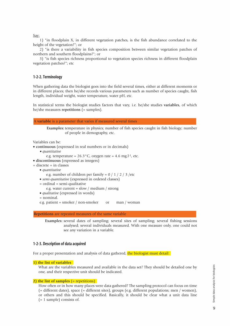
By convention variables are presented as columns, and samples (or repetitions) as rows:

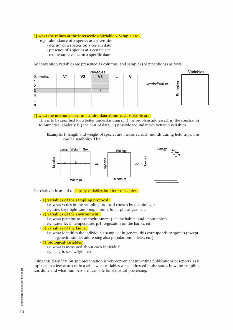
4) what the methods used to acquire data about each variable areThis is to be specified for a better understanding of i) the problem addressed; ii) the constraintsto numerical analysis; iii) the cost of data; iv) possible redundancies between variables.

Example: If length and weight of species are measured each month during field trips, this can be symbolized by:

For clarity it is useful to classify variables into four categories:

- 1) variables of the sampling protocoli.e. what varies in the sampling protocol chosen by the biologiste.g. site, day/night sampling; month, lunar phase, gear, etc.

- 2) variables of the environmenti.e. what pertains to the environment (i.e. the habitat and its variables)e.g. water level, temperature, pH, vegetation on the banks, etc.

- 3) variables of the faunai.e. what identifies the individuals sampled; in general this corresponds to species (except

in genetics studies addressing also populations, alleles, etc.)- 4) biological variables

i.e. what is measured about each individuale.g. length, sex, weight, etc.

Using this classification and presentation is very convenient in writing publications or reports, as itexplains in a few words or in a table what variables were addressed in the study, how the samplingwas done and what numbers are available for statistical processing.

10

Sim

ple

dat

a an

alys

is fo

r b

iolo

gis

ts

Example:

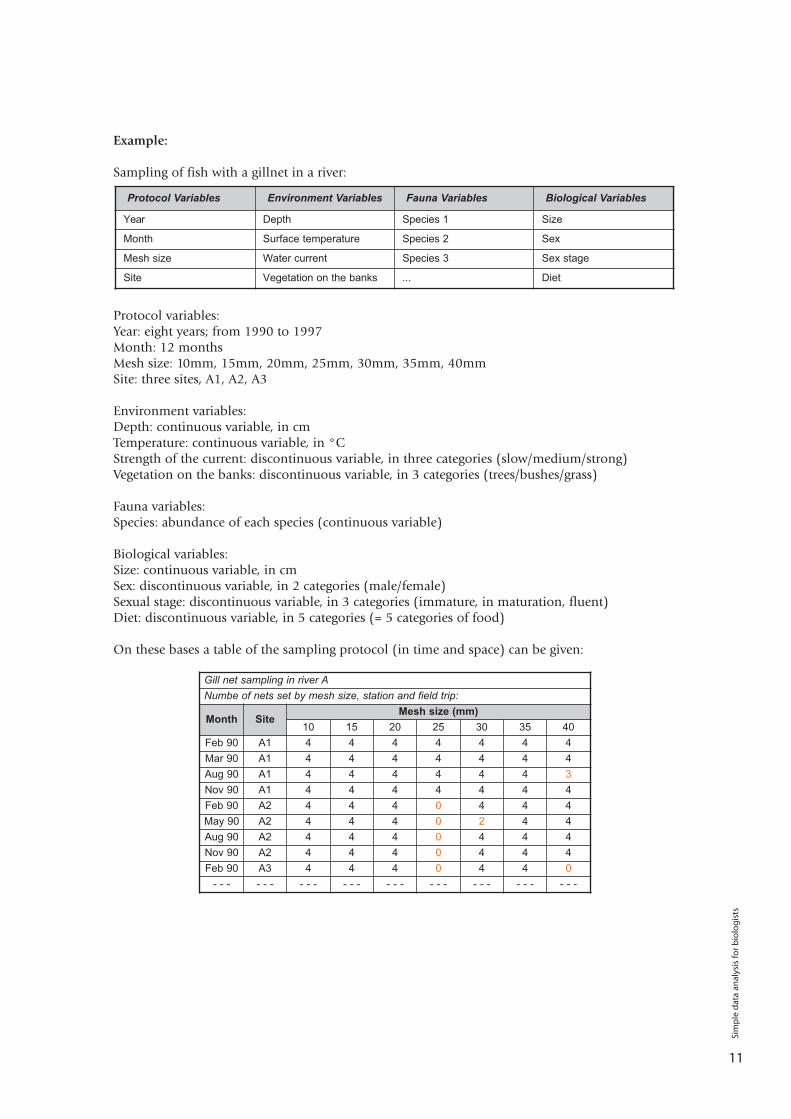
Sampling of fish with a gillnet in a river:

Protocol variables:Year: eight years; from 1990 to 1997Month: 12 monthsMesh size: 10mm, 15mm, 20mm, 25mm, 30mm, 35mm, 40mmSite: three sites, A1, A2, A3

Environment variables:Depth: continuous variable, in cmTemperature: continuous variable, in °CStrength of the current: discontinuous variable, in three categories (slow/medium/strong)Vegetation on the banks: discontinuous variable, in 3 categories (trees/bushes/grass)

Fauna variables:Species: abundance of each species (continuous variable)

Biological variables:Size: continuous variable, in cmSex: discontinuous variable, in 2 categories (male/female)Sexual stage: discontinuous variable, in 3 categories (immature, in maturation, fluent)Diet: discontinuous variable, in 5 categories (= 5 categories of food)

On these bases a table of the sampling protocol (in time and space) can be given:

Gill net sampling in river ANumbe of nets set by mesh size, station and field trip:

Month SiteMesh size (mm)

10 15 20 25 30 35 40Feb 90 A1 4 4 4 4 4 4 4Mar 90 A1 4 4 4 4 4 4 4Aug 90 A1 4 4 4 4 4 4 3Nov 90 A1 4 4 4 4 4 4 4Feb 90 A2 4 4 4 0 4 4 4May 90 A2 4 4 4 0 2 4 4Aug 90 A2 4 4 4 0 4 4 4Nov 90 A2 4 4 4 0 4 4 4Feb 90 A3 4 4 4 0 4 4 0

- - - - - - - - - - - - - - - - - - - - - - - - - - -

Protocol Variables Environment Variables Fauna Variables Biological Variables

Year Depth Species 1 Size

Month Surface temperature Species 2 Sex

Mesh size Water current Species 3 Sex stage

Site Vegetation on the banks ... Diet

11

Sim

ple

dat

a an

alys

is fo

r b

iolo

gis

ts

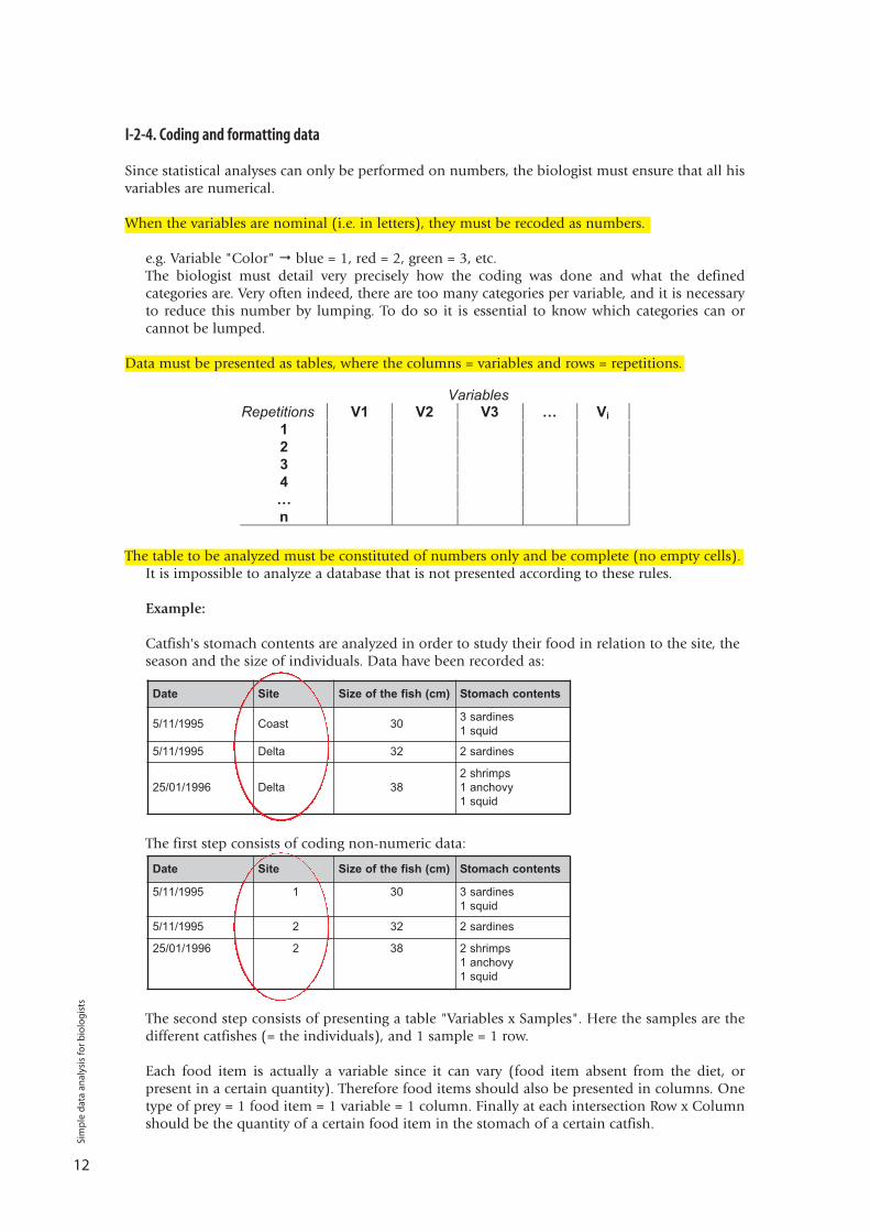
I-2-4. Coding and formatting data

Since statistical analyses can only be performed on numbers, the biologist must ensure that all hisvariables are numerical.

When the variables are nominal (i.e. in letters), they must be recoded as numbers.

e.g. Variable "Color" blue = 1, red = 2, green = 3, etc. The biologist must detail very precisely how the coding was done and what the definedcategories are. Very often indeed, there are too many categories per variable, and it is necessaryto reduce this number by lumping. To do so it is essential to know which categories can orcannot be lumped.

Data must be presented as tables, where the columns = variables and rows = repetitions.

The table to be analyzed must be constituted of numbers only and be complete (no empty cells). It is impossible to analyze a database that is not presented according to these rules.

Example:

Catfish's stomach contents are analyzed in order to study their food in relation to the site, theseason and the size of individuals. Data have been recorded as:

The first step consists of coding non-numeric data:

The second step consists of presenting a table "Variables x Samples". Here the samples are thedifferent catfishes (= the individuals), and 1 sample = 1 row.

Each food item is actually a variable since it can vary (food item absent from the diet, orpresent in a certain quantity). Therefore food items should also be presented in columns. Onetype of prey = 1 food item = 1 variable = 1 column. Finally at each intersection Row x Columnshould be the quantity of a certain food item in the stomach of a certain catfish.

Date Site Size of the fish (cm) Stomach contents

5/11/1995 1 30 3 sardines1 squid

5/11/1995 2 32 2 sardines

25/01/1996 2 38 2 shrimps1 anchovy1 squid

Date Site Size of the fish (cm) Stomach contents

5/11/1995 Coast 30 3 sardines1 squid

5/11/1995 Delta 32 2 sardines

25/01/1996 Delta 382 shrimps1 anchovy1 squid

12

Sim

ple

dat

a an

alys

is fo

r b

iolo

gis

ts

Hence the final data table:

Only this final table can be processed for a statistical analysis; the previous table formats areintermediate stages that do not allow proper data analysis.

1-2-5. Translating biological questions into statistical questions

Although biological questions can be clear, they have to be translated into statistical questions, i.e.questions about data and no longer about biology or ecology. Therefore the biological questionsmust be reformulated in terms of correlations or statistical tests between rows, columns or tables.

Example:biological question: "is fish more abundant in coral reefs that feature high species diversity?"statistical question: - "is there a correlation between fish biomass and coral reef species

richness?"or, better: - "is there a correlation between fish catch per unit effort (CPUE) and

the coral species richness in different reefs?"

1-2-6. Amount of data required

Quality increases with quantityA fundamental issue in data analysis is: how much data should be gathered or analyzed to answera biological question?

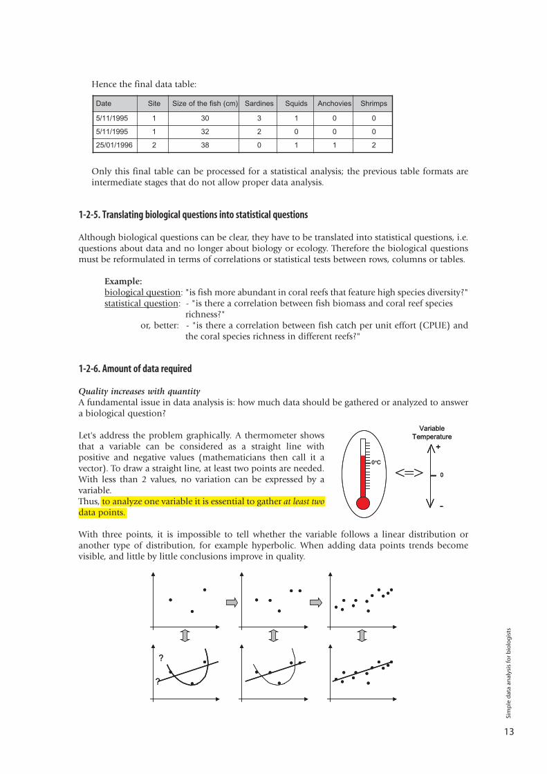
Let's address the problem graphically. A thermometer showsthat a variable can be considered as a straight line withpositive and negative values (mathematicians then call it avector). To draw a straight line, at least two points are needed.With less than 2 values, no variation can be expressed by avariable.Thus, to analyze one variable it is essential to gather at least twodata points.

With three points, it is impossible to tell whether the variable follows a linear distribution oranother type of distribution, for example hyperbolic. When adding data points trends becomevisible, and little by little conclusions improve in quality.

Date Site Size of the fish (cm) Sardines Squids Anchovies Shrimps

5/11/1995 1 30 3 1 0 0

5/11/1995 1 32 2 0 0 0

25/01/1996 2 38 0 1 1 2

13

Sim

ple

dat

a an

alys

is fo

r b

iolo

gis

ts

So the quality of the mathematical description of a phenomenon depends on the number of pointsexpressing the variables. Consequently, there is no threshold in the amount of data required toanswer a question.

Instead there should be a certain ratio between the number of variables studied and the number ofmeasurements (= of samples).

Ratio between variables studied and data gatheredThe quality of conclusions drawn from data depends on the ratio between the number of variablesand the number of data points measured. For instance, conclusions about the average age,education level and income in a village (i.e. 3 variables) will be relatively good if at least 30villagers are interviewed, but they will not be acceptable if only 5 villagers are interviewed. The ratiobetween "number of variables" and "number of samples" is an essential quality criterion.

As a rule of thumb, when studying n variables it is not acceptable to draw conclusions from lessthan 5n samples.

Exploratory statisticsIn exploratory statistics (= multivariate analyses), data and conclusions are good when there are atleast 10n samples to study n variables.

Parametric testsIn order to perform parametric tests (assuming a certain distribution) on variables or betweenvariables, at least 30 data points per variable are required.

Non-parametric testsThe minimum amount of data required to perform non-parametric tests is 6 data points pervariable.

Total number of variables studiedIn fact the number of data points or samples is easy to assess, but the actual number of variablesrequires more attention.

Identification of hidden variablesThe best way to identify all variables is to ask:

"What are the factors that can vary from a sample to another?" Each of them is a variable.

Example:Fish sampling was undertaken in 5 villages with two gears (gillnets and traps) in order toidentify fish species present in each place. It is clear that the main variables are Location(5 villages), Gear (gillnet or trap), and Fish species, However in each village two types ofenvironments were sampled: wetlands and river mainstream. Also gillnets are made of threemesh sizes (small, medium, large) to catch the whole range of fish sizes. So instead of threevariables, there are actually five variables. They can be identified by asking the question:"What are the factors that can vary from a sample to another?", i.e. i) Location (5 villages);ii) Environment (wetland or mainstream); iii) Gear (gillnet or trap); iv) Mesh size (small,medium or large), and v) Fish species.

Identification of variable categories as independent variablesWhen a variable is discontinuous, i.e. expressed in classes (e.g. colour: green/yellow/red), each classactually counts as one variable by the software running the numerical analysis. It is thus necessaryto transform each discontinuous variable including n classes into n columns of codes 0 and 1 only.This process is automated in most statistical packages.

Each class of a discontinuous variable must be considered as ONE variableAs a consequence the total number of variables involved in the analysis often increases drastically,and the ratio Number of samples / Number of variables becomes insufficient for proper analysis.

14

Sim

ple

dat

a an

alys

is fo

r b

iolo

gis

ts

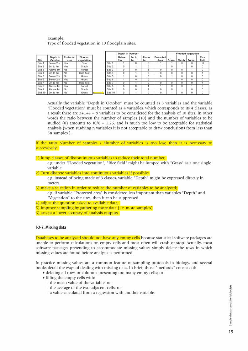
Example:Type of flooded vegetation in 10 floodplain sites:

Actually the variable "Depth in October" must be counted as 3 variables and the variable"Flooded vegetation" must be counted as 4 variables, which corresponds to its 4 classes; asa result there are 3+1+4 = 8 variables to be considered for the analysis of 10 sites. In otherwords the ratio between the number of samples (10) and the number of variables to bestudied (8) amounts to 10/8 = 1.25, and is much too low to be acceptable for statisticalanalysis (when studying n variables it is not acceptable to draw conclusions from less than5n samples.).

If the ratio Number of samples / Number of variables is too low, then it is necessary tosuccessively:

1) lump classes of discontinuous variables to reduce their total number;e.g. under "Flooded vegetation", "Rice field" might be lumped with "Grass" as a one singlevariable

2) Turn discrete variables into continuous variables if possible; e.g. instead of being made of 3 classes, variable "Depth" might be expressed directly inmeters

3) make a selection in order to reduce the number of variables to be analyzed;e.g. if variable "Protected area" is considered less important than variables "Depth" and"Vegetation" to the sites, then it can be suppressed

4) adjust the question asked to available data;5) improve sampling by gathering more data (i.e. more samples)6) accept a lower accuracy of analysis outputs.

I-2-7. Missing data

Databases to be analyzed should not have any empty cells because statistical software packages areunable to perform calculations on empty cells and most often will crash or stop. Actually, mostsoftware packages pretending to accommodate missing values simply delete the rows in whichmissing values are found before analysis is performed.

In practice missing values are a common feature of sampling protocols in biology, and severalbooks detail the ways of dealing with missing data. In brief, those "methods" consists of:

• deleting all rows or columns presenting too many empty cells; or• filling the empty cells with:

- the mean value of the variable; or- the average of the two adjacent cells; or- a value calculated from a regression with another variable.

Depth in OctoberProtected

Area

Flooded vegetationBelow2m

2m to4m

Above4m Grass Shrub Forest

Ricefield

Site 1 1 0 0 1 1 0 0 0Site 2 0 1 0 1 0 1 0 0Site 3 0 0 1 0 0 0 1 0Site 4 0 1 0 0 0 0 0 1Site 5 1 0 0 0 1 0 0 0Site 6 1 0 0 1 1 0 0 0Site 7 0 1 0 0 0 0 0 1Site 8 0 0 1 1 0 0 1 0Site 9 0 0 1 0 0 1 0 0Site 10 0 1 0 0 1 0 0 0

SiteDepth inOctober

Protectedarea

Floodedvegetation

Site 1 Below 2m Yes GrasSite 2 2m to 4m Yes ShrubSite 3 Above 4m No ForestSite 4 2m to 4m No Rice fieldSite 5 Below 2m No GrassSite 6 Below 2m Yes GrassSite 7 2m to 4m No Rice fieldSite 8 Above 4m Yes ForestSite 9 Above 4m No ShrubSite 10 2m to 4m No Grass

15

Sim

ple

dat

a an

alys

is fo

r b

iolo

gis

ts

2-1. MENU CUSTOMIZATION

Some tools in Excel are very useful and should always be at hand. The procedure to put them onyour main toolbar is as follows:

Menu

Drag the button you want from the Commands box to the toolbar on the top of your Word page.

The commands you need to have on your main toolbar are:

Category Edit • Paste Values (pastes only the values from the copied cells into the selected cells)• Paste Format (pastes only the format of the copied cells into the selected cells)• Down (copies the contents and format of the topmost cell of a selected range into the cells

below)• Right (copies the contents and format of the leftmost cell of a selected range into the right

selected cells)• Clear (deletes the selected object or text without putting it on the Clipboard.

This command is available only if an object or text is selected) • Clear Formatting (removes only the format from selected cells; cell contents and notes

remain unchanged)

CommandsCustomize

Tools

In the box, click a category (here Edit)Categoriestab.

2 USING MS EXCEL FORDATA ANALYSIS

16

Sim

ple

dat

a an

alys

is fo

r b

iolo

gis

ts

Category Insert• Chart• Paste Function • Autosum• Increase decimal• Decrease decimal

Category Data• PivotTable and PivotChart Report

Your standard toolbar should ultimately look like this:

17

Sim

ple

dat

a an

alys

is fo

r b

iolo

gis

ts

18

2-2. SORTING DATA

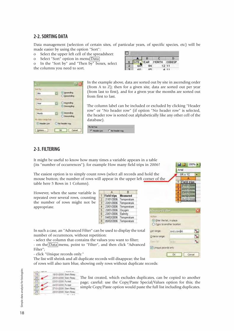
Data management (selection of certain sites, of particular years, of specific species, etc) will bemade easier by using the option "Sort":o Select the upper left cell of the spreadsheet:o Select "Sort" option in menu Datao In the "Sort by" and "Then by" boxes, selectthe columns you need to sort.

In the example above, data are sorted out by site in ascending order(from A to Z); then for a given site, data are sorted out per year(from last to first), and for a given year the months are sorted outfrom first to last.

The column label can be included or excluded by clicking "Headerrow" or "No header row" (if option "No header row" is selected,the header row is sorted out alphabetically like any other cell of thedatabase).

2-3. FILTERING

It might be useful to know how many times a variable appears in a table(its "number of occurrences"); for example How many field trips in 2006?

The easiest option is to simply count rows (select all records and hold themouse button; the number of rows will appear in the upper left corner of thetable here 5 Rows in 1 Column).

However, when the same variable isrepeated over several rows, countingthe number of rows might not beappropriate.

In such a case, an "Advanced Filter" can be used to display the totalnumber of occurrences, without repetition:- select the column that contains the values you want to filter;- on the Data menu, point to "Filter", and then click "AdvancedFilter";- click "Unique records only."The list will shrink and all duplicate records will disappear; the listof rows will also turn blue, showing only rows without duplicate records:

The list created, which excludes duplicates, can be copied to anotherpage; careful: use the Copy/Paste Special/Values option for this; thesimple Copy/Paste option would paste the full list including duplicates.

Sim

ple

dat

a an

alys

is fo

r b

iolo

gis

ts

19

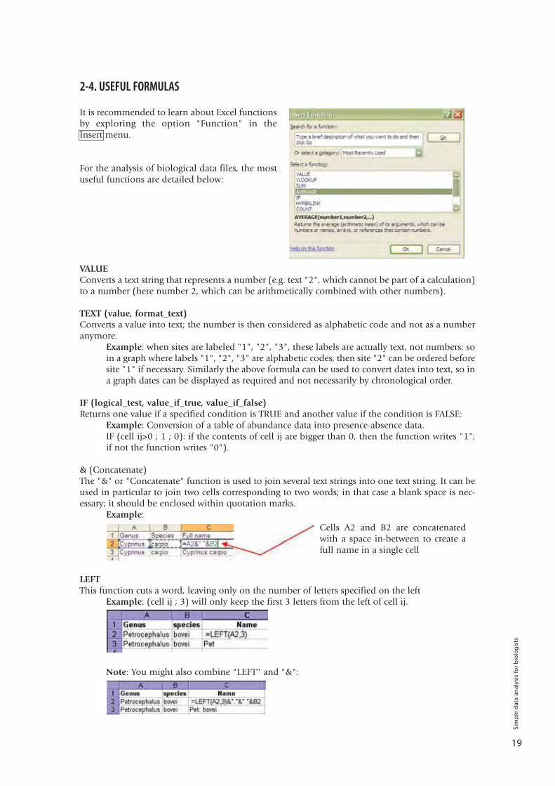
2-4. USEFUL FORMULAS

It is recommended to learn about Excel functionsby exploring the option "Function" in theInsert menu.

For the analysis of biological data files, the mostuseful functions are detailed below:

VALUEConverts a text string that represents a number (e.g. text "2", which cannot be part of a calculation)to a number (here number 2, which can be arithmetically combined with other numbers).

TEXT (value, format_text)Converts a value into text; the number is then considered as alphabetic code and not as a numberanymore.

Example: when sites are labeled "1", "2", "3", these labels are actually text, not numbers; soin a graph where labels "1", "2", "3" are alphabetic codes, then site "2" can be ordered beforesite "1" if necessary. Similarly the above formula can be used to convert dates into text, so ina graph dates can be displayed as required and not necessarily by chronological order.

IF (logical_test, value_if_true, value_if_false) Returns one value if a specified condition is TRUE and another value if the condition is FALSE:

Example: Conversion of a table of abundance data into presence-absence data.IF (cell ij>0 ; 1 ; 0): if the contents of cell ij are bigger than 0, then the function writes "1";if not the function writes "0").

& (Concatenate)The "&" or "Concatenate" function is used to join several text strings into one text string. It can beused in particular to join two cells corresponding to two words; in that case a blank space is nec-essary; it should be enclosed within quotation marks.

Example:

LEFTThis function cuts a word, leaving only on the number of letters specified on the left

Example: (cell ij ; 3) will only keep the first 3 letters from the left of cell ij.

Note: You might also combine "LEFT" and "&":

Cells A2 and B2 are concatenatedwith a space in-between to create afull name in a single cell

Sim

ple

dat

a an

alys

is fo

r b

iolo

gis

ts

20

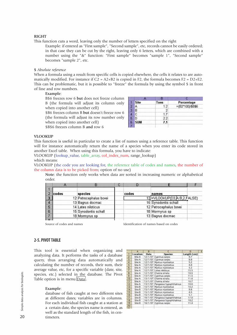
RIGHTThis function cuts a word, leaving only the number of letters specified on the right

Example: if entered as "First sample", "Second sample", etc, records cannot be easily ordered;in that case they can be cut by the right, leaving only 6 letters, which are combined with anumber using the "&" function: "First sample" becomes "sample 1", "Second sample"becomes "sample 2", etc.

$ Absolute referenceWhen a formula using a result from specific cells is copied elsewhere, the cells it relates to are auto-matically modified. For instance if C2 = A2+B2 is copied in F2, the formula becomes F2 = D2+E2.This can be problematic, but it is possible to "freeze" the formula by using the symbol $ in frontof line and row numbers.

Example:B$6 freezes row 6 but does not freeze columnB (the formula will adjust its column onlywhen copied into another cell) $B6 freezes column B but doesn't freeze row 6(the formula will adjust its row number onlywhen copied into another cell) $B$6 freezes column B and row 6

VLOOKUPThis function is useful in particular to create a list of names using a reference table. This functionwill for instance automatically return the name of a species when you enter its code stored inanother Excel table. When using this formula, you have to indicate:VLOOKUP (lookup_value, table_array, col_index_num, range_lookup)which means:VLOOKUP (the code you are looking for, the reference table of codes and names, the number ofthe column data is to be picked from; option of no use)

Note: the function only works when data are sorted in increasing numeric or alphabeticalorder.

Source of codes and names Identification of names based on codes

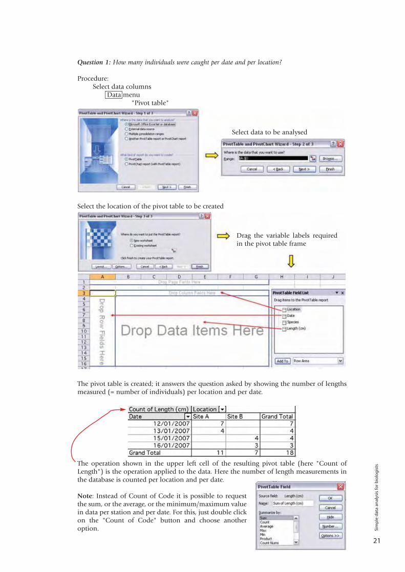
2-5. PIVOT TABLE

This tool is essential when organizing andanalyzing data. It performs the tasks of a databasequery, thus arranging data automatically andcalculating the number of records, their sum, theiraverage value, etc, for a specific variable (date, site,species, etc.) selected in the database. The PivotTable option is in menu Data .

Example:database of fish caught at two different sitesat different dates; variables are in columns.For each individual fish caught at a station ata certain date, the species name is entered, aswell as the standard length of the fish, in cen-timeters.

Sim

ple

dat

a an

alys

is fo

r b

iolo

gis

ts

21

Question 1: How many individuals were caught per date and per location?

Procedure:Select data columns

Data menu"Pivot table"

Select the location of the pivot table to be created

The pivot table is created; it answers the question asked by showing the number of lengthsmeasured (= number of individuals) per location and per date.

The operation shown in the upper left cell of the resulting pivot table (here "Count ofLength") is the operation applied to the data. Here the number of length measurements inthe database is counted per location and per date.

Note: Instead of Count of Code it is possible to requestthe sum, or the average, or the minimum/maximum valuein data per station and per date. For this, just double clickon the "Count of Code" button and choose anotheroption.

Drag the variable labels requiredin the pivot table frame

Select data to be analysed

Sim

ple

dat

a an

alys

is fo

r b

iolo

gis

ts

22

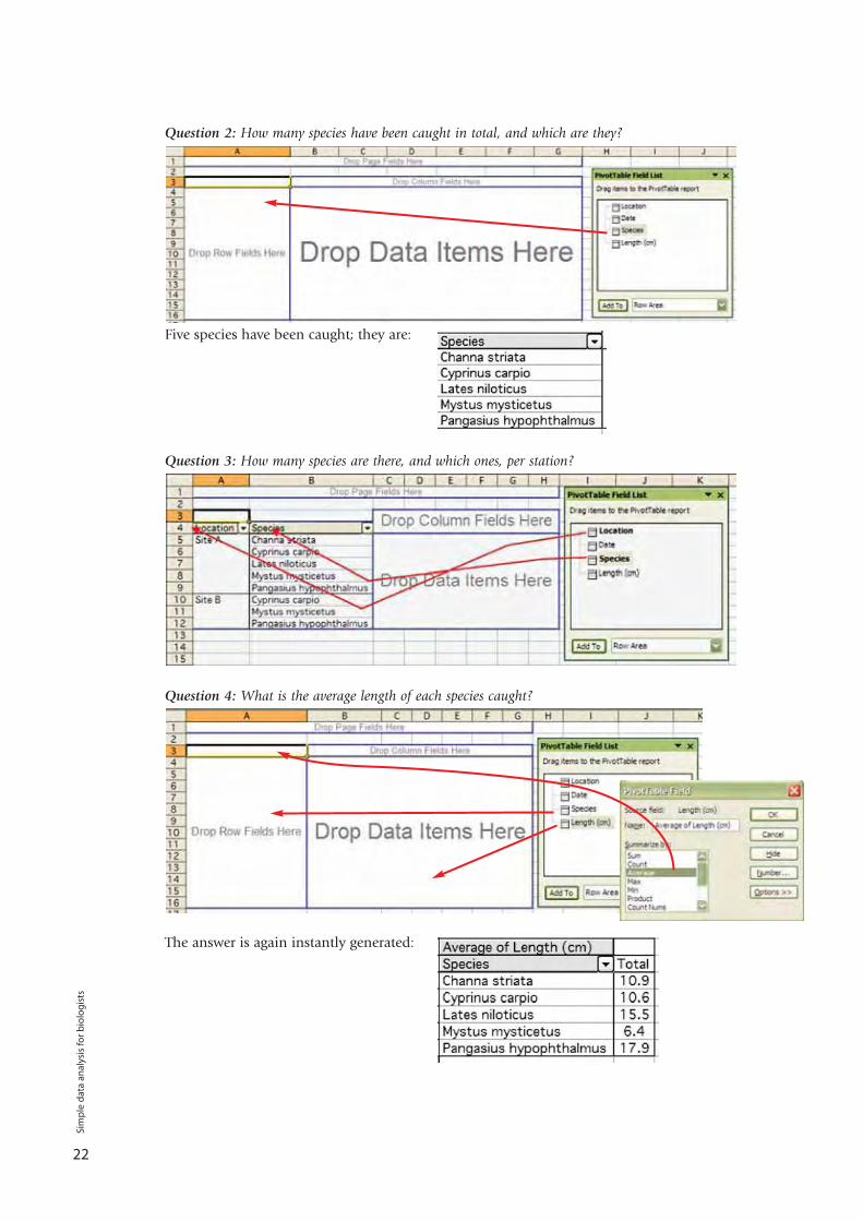
Question 2: How many species have been caught in total, and which are they?

Five species have been caught; they are:

Question 3: How many species are there, and which ones, per station?

Question 4: What is the average length of each species caught?

The answer is again instantly generated:

Sim

ple

dat

a an

alys

is fo

r b

iolo

gis

ts

23

2-6. CHARTS

This section is intended to highlight useful and often overlooked features available in the MS Excelchart options.

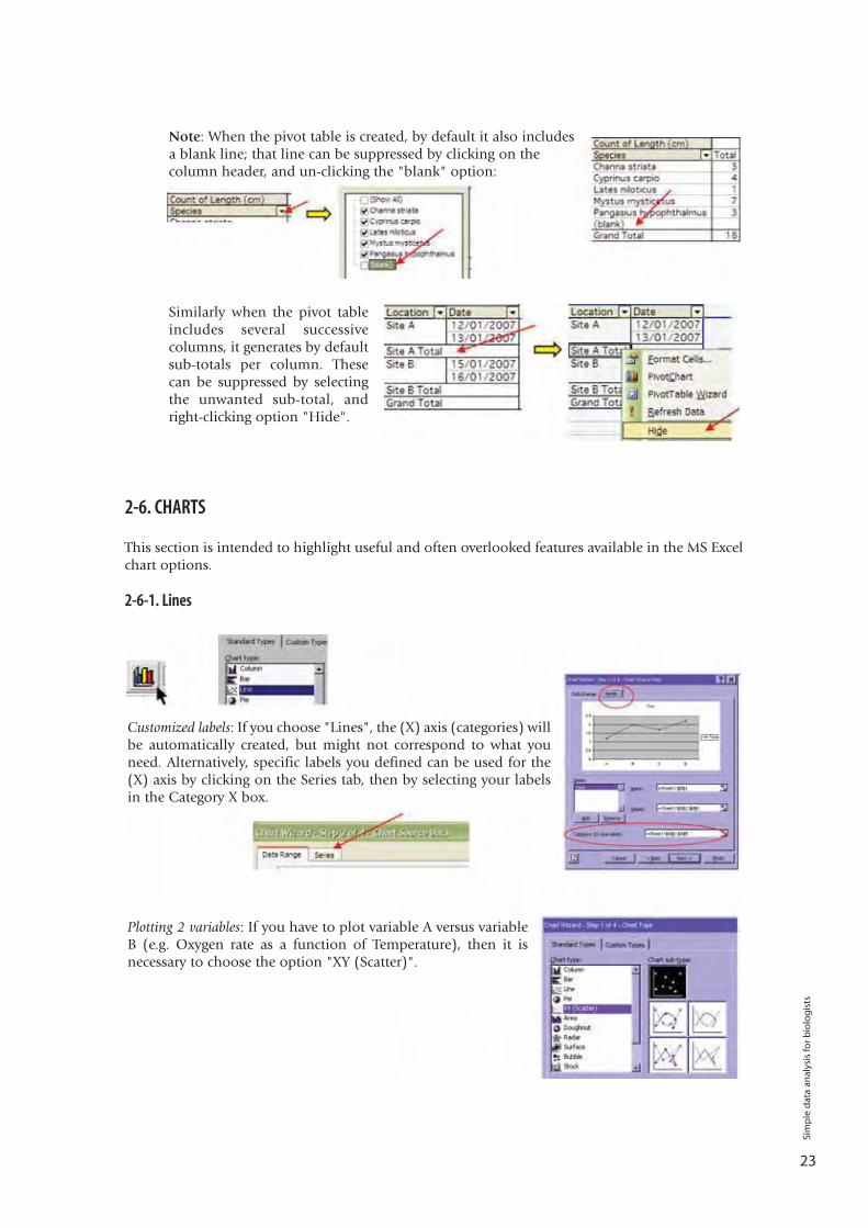
2-6-1. Lines

Customized labels: If you choose "Lines", the (X) axis (categories) willbe automatically created, but might not correspond to what youneed. Alternatively, specific labels you defined can be used for the(X) axis by clicking on the Series tab, then by selecting your labelsin the Category X box.

Plotting 2 variables: If you have to plot variable A versus variableB (e.g. Oxygen rate as a function of Temperature), then it isnecessary to choose the option "XY (Scatter)".

Similarly when the pivot tableincludes several successivecolumns, it generates by defaultsub-totals per column. Thesecan be suppressed by selectingthe unwanted sub-total, andright-clicking option "Hide".

Note: When the pivot table is created, by default it also includesa blank line; that line can be suppressed by clicking on thecolumn header, and un-clicking the "blank" option:

Sim

ple

dat

a an

alys

is fo

r b

iolo

gis

ts

24

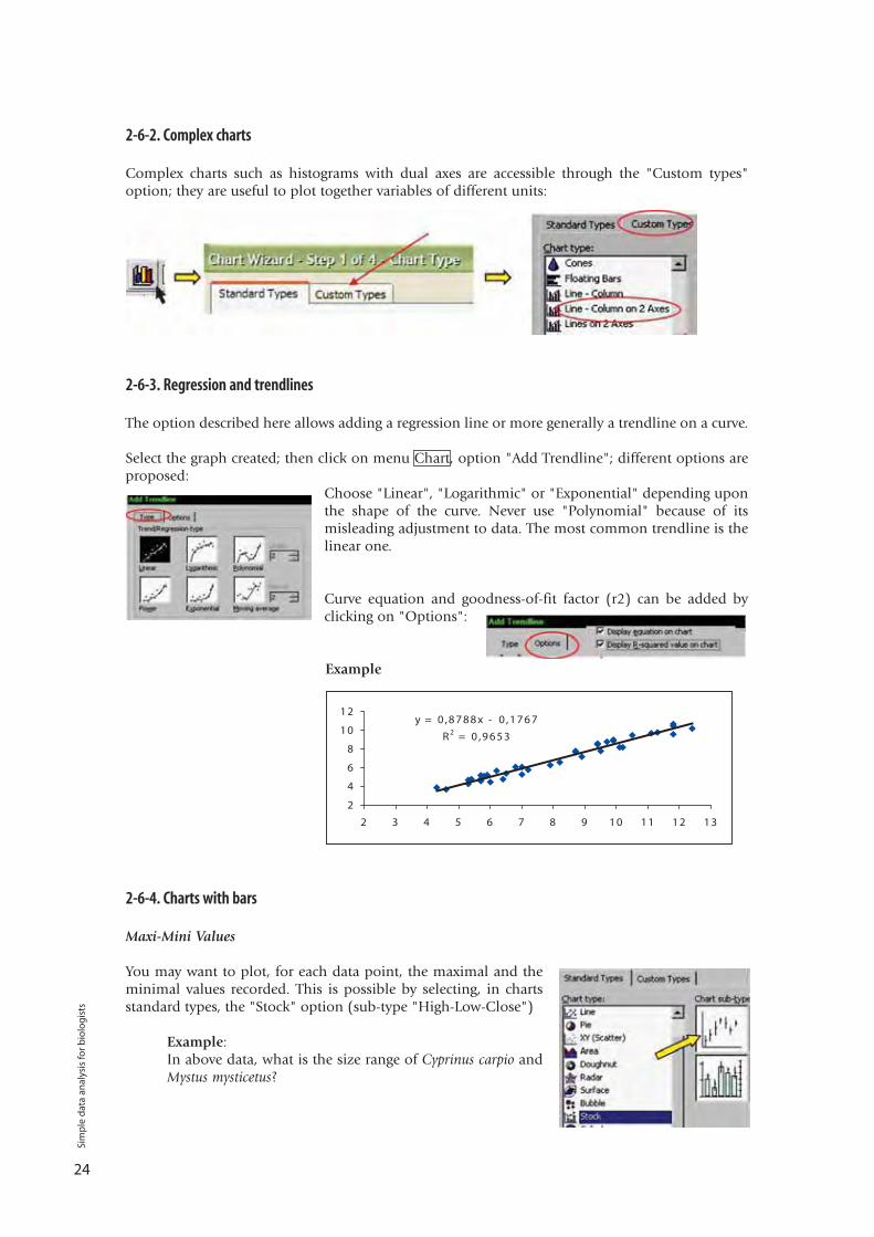
2-6-2. Complex charts

Complex charts such as histograms with dual axes are accessible through the "Custom types"option; they are useful to plot together variables of different units:

2-6-3. Regression and trendlines

The option described here allows adding a regression line or more generally a trendline on a curve.

Select the graph created; then click on menu Chart, option "Add Trendline"; different options areproposed:

Choose "Linear", "Logarithmic" or "Exponential" depending uponthe shape of the curve. Never use "Polynomial" because of itsmisleading adjustment to data. The most common trendline is thelinear one.

Curve equation and goodness-of-fit factor (r2) can be added byclicking on "Options":

Example

2-6-4. Charts with bars

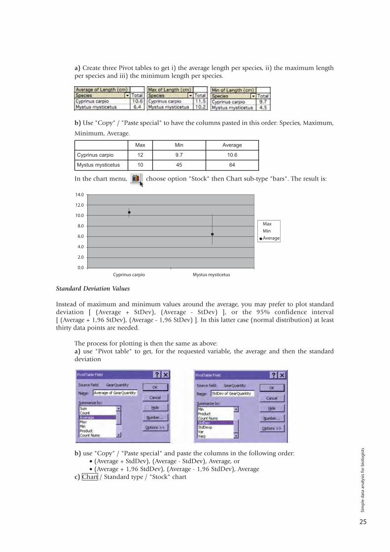
Maxi-Mini Values

You may want to plot, for each data point, the maximal and theminimal values recorded. This is possible by selecting, in chartsstandard types, the "Stock" option (sub-type "High-Low-Close")

Example:In above data, what is the size range of Cyprinus carpio andMystus mysticetus?

Sim

ple

dat

a an

alys

is fo

r b

iolo

gis

ts

25

a) Create three Pivot tables to get i) the average length per species, ii) the maximum lengthper species and iii) the minimum length per species.

b) Use "Copy" / "Paste special" to have the columns pasted in this order: Species, Maximum,

Minimum, Average.

In the chart menu, choose option "Stock" then Chart sub-type "bars". The result is:

Standard Deviation Values

Instead of maximum and minimum values around the average, you may prefer to plot standarddeviation [ (Average + StDev), (Average - StDev) ], or the 95% confidence interval[ (Average + 1,96 StDev), (Average - 1,96 StDev) ]. In this latter case (normal distribution) at leastthirty data points are needed.

The process for plotting is then the same as above:a) use "Pivot table" to get, for the requested variable, the average and then the standarddeviation

b) use "Copy" / "Paste special" and paste the columns in the following order: • (Average + StdDev), (Average - StdDev), Average, or• (Average + 1,96 StdDev), (Average - 1,96 StdDev), Average

c) Chart / Standard type / "Stock" chart

Max Min Average

Cyprinus carpio 12 9.7 10.6

Mystus mysticetus 10 45 64

Sim

ple

dat

a an

alys

is fo

r b

iolo

gis

ts

26

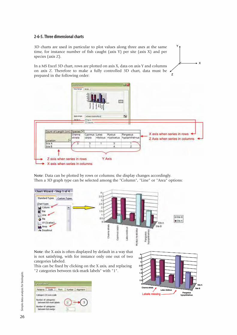
2-6-5. Three dimensional charts

3D charts are used in particular to plot values along three axes at the sametime, for instance number of fish caught (axis Y) per site (axis X) and perspecies (axis Z).

In a MS Excel 3D chart, rows are plotted on axis X, data on axis Y and columnson axis Z. Therefore to make a fully controlled 3D chart, data must beprepared in the following order:

Note: Data can be plotted by rows or columns; the display changes accordingly.Then a 3D graph type can be selected among the "Column", "Line" or "Area" options:

Note: the X axis is often displayed by default in a way thatis not satisfying, with for instance only one out of twocategories labeled.This can be fixed by clicking on the X axis, and replacing "2 categories between tick-mark labels" with "1".

Sim

ple

dat

a an

alys

is fo

r b

iolo

gis

ts

27

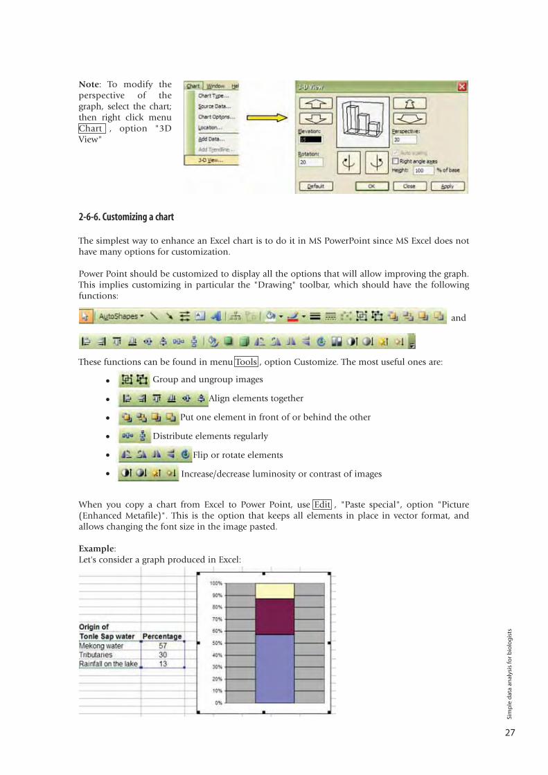
Note: To modify theperspective of thegraph, select the chart;then right click menuChart , option "3DView"

2-6-6. Customizing a chart

The simplest way to enhance an Excel chart is to do it in MS PowerPoint since MS Excel does nothave many options for customization.

Power Point should be customized to display all the options that will allow improving the graph.This implies customizing in particular the "Drawing" toolbar, which should have the followingfunctions:

and

These functions can be found in menu Tools , option Customize. The most useful ones are:

Group and ungroup images

Align elements together

Put one element in front of or behind the other

Distribute elements regularly

Flip or rotate elements

Increase/decrease luminosity or contrast of images

When you copy a chart from Excel to Power Point, use Edit , "Paste special", option "Picture(Enhanced Metafile)". This is the option that keeps all elements in place in vector format, andallows changing the font size in the image pasted.

Example:Let's consider a graph produced in Excel:

•

•

•

•

•

•

Sim

ple

dat

a an

alys

is fo

r b

iolo

gis

ts

28

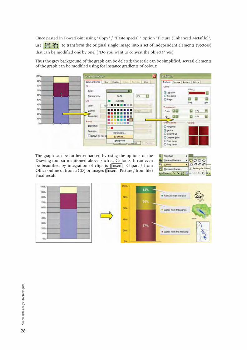
Once pasted in PowerPoint using "Copy" / "Paste special," option "Picture (Enhanced Metafile)",

use to transform the original single image into a set of independent elements (vectors)

that can be modified one by one. ("Do you want to convert the object?" Yes)

Thus the grey background of the graph can be deleted; the scale can be simplified, several elementsof the graph can be modified using for instance gradients of colour:

The graph can be further enhanced by using the options of theDrawing toolbar mentioned above, such as Callouts. It can evenbe beautified by integration of cliparts (Insert , Clipart / fromOffice online or from a CD) or images (Insert , Picture / from file)Final result:

Sim

ple

dat

a an

alys

is fo

r b

iolo

gis

ts

29

Sim

ple

dat

a an

alys

is fo

r b

iolo

gis

ts

Exploratory analysis consists of analyzing data about a situation or environment that is not wellknown and that often involves several variables. For instance:- the response of an aquatic species to its environment (several environmental variables);- the distribution of fish species (several species as variables) in a river;- the behaviour of consumers (many individuals as variables) in response to a given socio-economic context (multiple social and environmental variables).

The tools used for exploratory analyses are mainly multivariate methods, i.e. statistical methodsdealing with many variables at the same time.

Note: One analysis, data analysis, but several analyses (irregular plural).

The two basic tools of exploratory analysis (= exploratory statistics) are the Principal ComponentAnalysis (PCA) and the Correspondence Analysis (CA or COA). These two methods are based onthe same fundamental principles. Their role is to visually summarize all analyzed variables, and toreveal their inter-relationships.

The principles are presented below following the French school of multivariate statistics (initiatedby Benzecri et al. in the 1970's), in which variables are expressed geometrically as vectors,correlations as angles between vectors and analyses are seen as projections of these vectors ontoplanes. Emphasis is given to this school as it is very graphic and has proven to be easily understoodby those who are not familiar or at ease with mathematics. However, this brief introduction shouldnot prevent the biologist from reading about the classical (i.e. arithmetical or analytical) approachof multivariate analyses, since geometric and arithmetical approaches are the two sides of the samecoin, and thus complement one another.

We do not detail here the way to run multivariate analyses with computer software (manuals detailthis procedure, which is program-specific), but rather how to understand the underlying principlesand interpret the outcomes of multivariate analyses, in particular the two basic ones: principalcomponent analysis and correspondence analysis.

3 UNDERSTANDINGEXPLORATORYANALYSIS OF DATA

30

Sim

ple

dat

a an

alys

is fo

r b

iolo

gis

ts

3-1. GEOMETRICAL APPROACH TO VARIABLES

3-1-1. Variables as dimensions

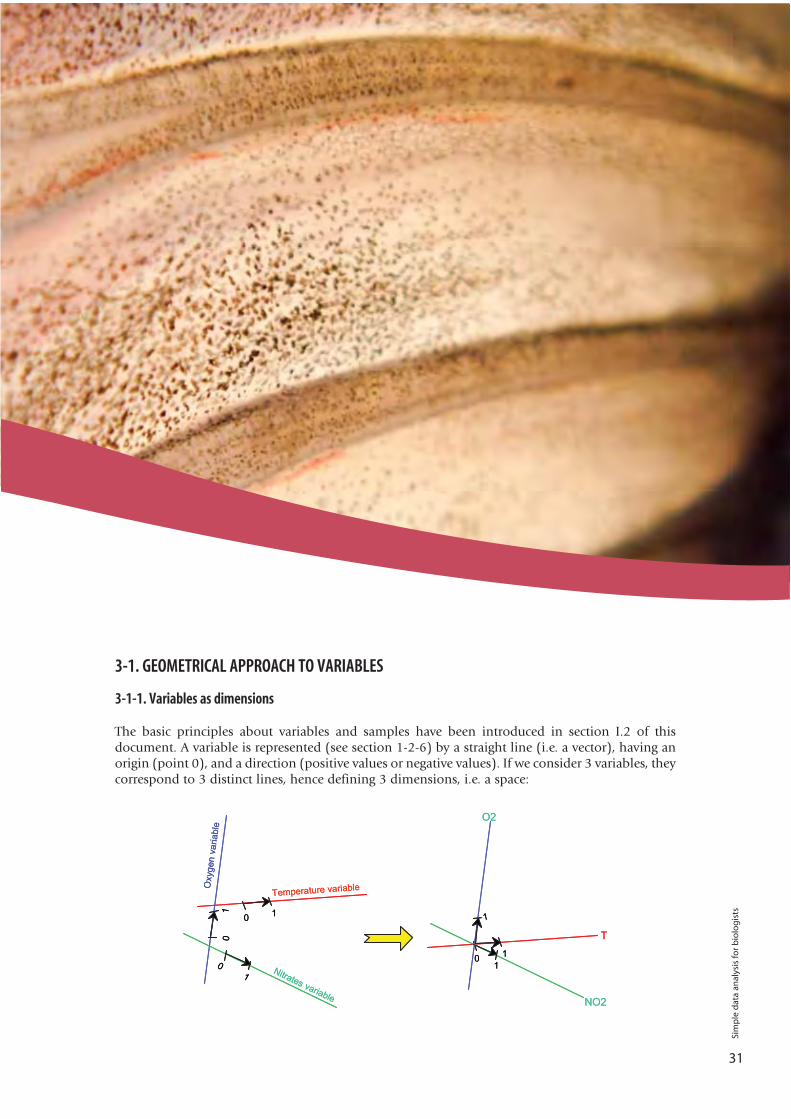
The basic principles about variables and samples have been introduced in section I.2 of thisdocument. A variable is represented (see section 1-2-6) by a straight line (i.e. a vector), having anorigin (point 0), and a direction (positive values or negative values). If we consider 3 variables, theycorrespond to 3 distinct lines, hence defining 3 dimensions, i.e. a space:

31

Sim

ple

dat

a an

alys

is fo

r b

iolo

gis

ts

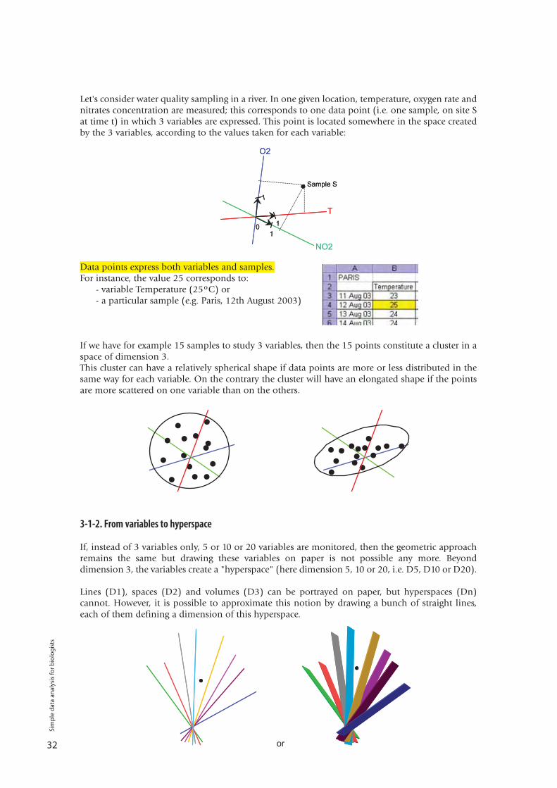
Let's consider water quality sampling in a river. In one given location, temperature, oxygen rate andnitrates concentration are measured; this corresponds to one data point (i.e. one sample, on site Sat time t) in which 3 variables are expressed. This point is located somewhere in the space createdby the 3 variables, according to the values taken for each variable:

Data points express both variables and samples. For instance, the value 25 corresponds to:

- variable Temperature (25ºC) or - a particular sample (e.g. Paris, 12th August 2003)

If we have for example 15 samples to study 3 variables, then the 15 points constitute a cluster in aspace of dimension 3. This cluster can have a relatively spherical shape if data points are more or less distributed in thesame way for each variable. On the contrary the cluster will have an elongated shape if the pointsare more scattered on one variable than on the others.

3-1-2. From variables to hyperspace

If, instead of 3 variables only, 5 or 10 or 20 variables are monitored, then the geometric approachremains the same but drawing these variables on paper is not possible any more. Beyonddimension 3, the variables create a "hyperspace" (here dimension 5, 10 or 20, i.e. D5, D10 or D20).

Lines (D1), spaces (D2) and volumes (D3) can be portrayed on paper, but hyperspaces (Dn)cannot. However, it is possible to approximate this notion by drawing a bunch of straight lines,each of them defining a dimension of this hyperspace.

32

Sim

ple

dat

a an

alys

is fo

r b

iolo

gis

ts

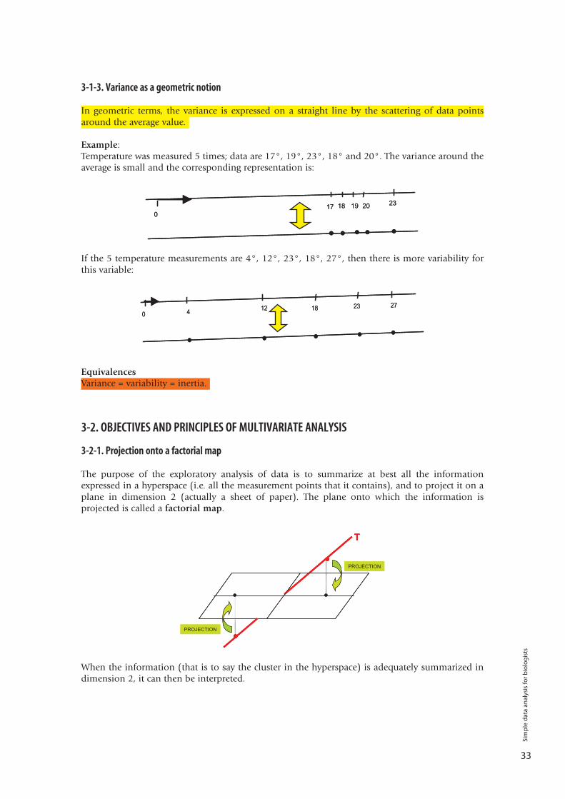
3-1-3. Variance as a geometric notion

In geometric terms, the variance is expressed on a straight line by the scattering of data pointsaround the average value.

Example:Temperature was measured 5 times; data are 17°, 19°, 23°, 18° and 20°. The variance around theaverage is small and the corresponding representation is:

If the 5 temperature measurements are 4°, 12°, 23°, 18°, 27°, then there is more variability forthis variable:

EquivalencesVariance = variability = inertia.

3-2. OBJECTIVES AND PRINCIPLES OF MULTIVARIATE ANALYSIS

3-2-1. Projection onto a factorial map

The purpose of the exploratory analysis of data is to summarize at best all the informationexpressed in a hyperspace (i.e. all the measurement points that it contains), and to project it on aplane in dimension 2 (actually a sheet of paper). The plane onto which the information isprojected is called a factorial map.

When the information (that is to say the cluster in the hyperspace) is adequately summarized indimension 2, it can then be interpreted.

33

Sim

ple

dat

a an

alys

is fo

r b

iolo

gis

ts

34

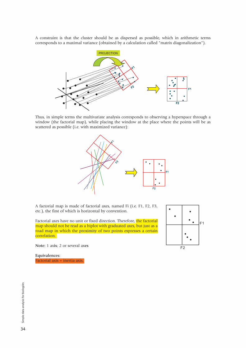
A constraint is that the cluster should be as dispersed as possible, which in arithmetic termscorresponds to a maximal variance (obtained by a calculation called "matrix diagonalization").

Thus, in simple terms the multivariate analysis corresponds to observing a hyperspace through awindow (the factorial map), while placing the window at the place where the points will be asscattered as possible (i.e. with maximized variance):

A factorial map is made of factorial axes, named Fi (i.e. F1, F2, F3,etc.), the first of which is horizontal by convention.

Factorial axes have no unit or fixed direction. Therefore, the factorialmap should not be read as a biplot with graduated axes, but just as aroad map in which the proximity of two points expresses a certaincorrelation.

Note: 1 axis; 2 or several axes

Equivalences:Factorial axis = inertia axis.

Sim

ple

dat

a an

alys

is fo

r b

iolo

gis

ts

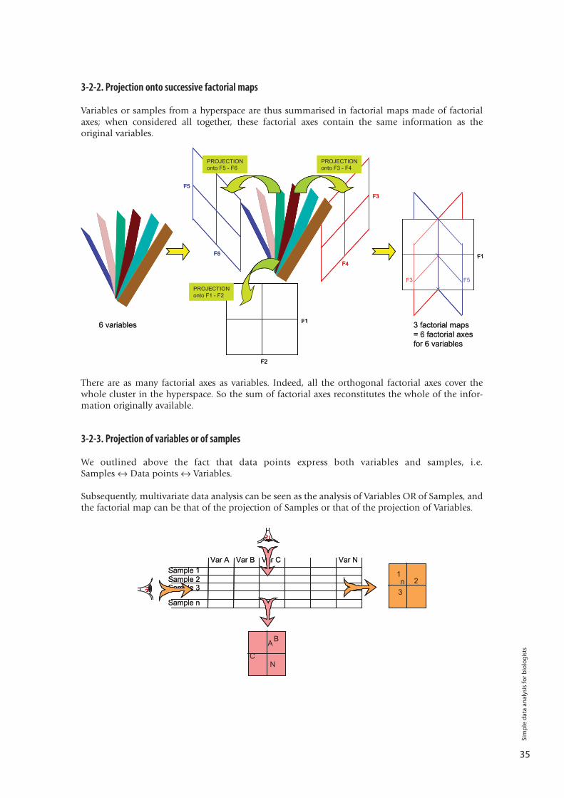
3-2-2. Projection onto successive factorial maps

Variables or samples from a hyperspace are thus summarised in factorial maps made of factorialaxes; when considered all together, these factorial axes contain the same information as theoriginal variables.

There are as many factorial axes as variables. Indeed, all the orthogonal factorial axes cover thewhole cluster in the hyperspace. So the sum of factorial axes reconstitutes the whole of the infor-mation originally available.

3-2-3. Projection of variables or of samples

We outlined above the fact that data points express both variables and samples, i.e. Samples ↔ Data points ↔ Variables.

Subsequently, multivariate data analysis can be seen as the analysis of Variables OR of Samples, andthe factorial map can be that of the projection of Samples or that of the projection of Variables.

35

Sim

ple

dat

a an

alys

is fo

r b

iolo

gis

ts

3-3. SOME PROPERTIES OF MULTIVARIATE ANALYSES

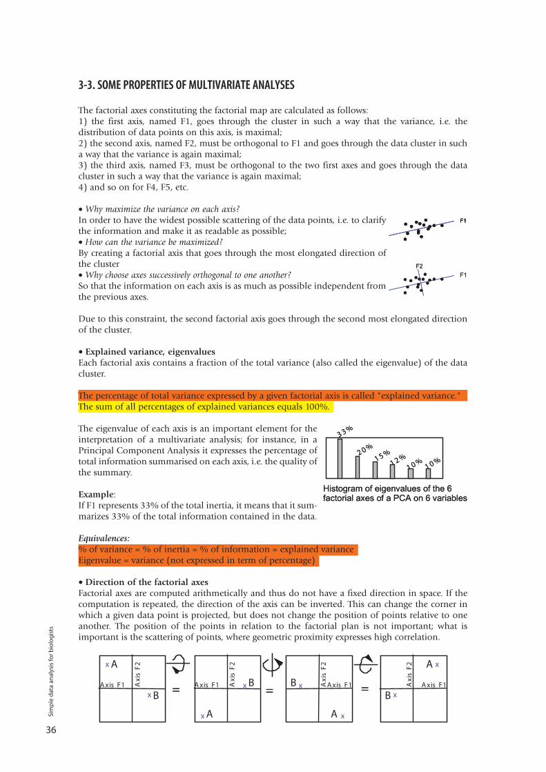
The factorial axes constituting the factorial map are calculated as follows: 1) the first axis, named F1, goes through the cluster in such a way that the variance, i.e. thedistribution of data points on this axis, is maximal;2) the second axis, named F2, must be orthogonal to F1 and goes through the data cluster in sucha way that the variance is again maximal;3) the third axis, named F3, must be orthogonal to the two first axes and goes through the datacluster in such a way that the variance is again maximal;4) and so on for F4, F5, etc.

• Why maximize the variance on each axis?In order to have the widest possible scattering of the data points, i.e. to clarifythe information and make it as readable as possible;• How can the variance be maximized?By creating a factorial axis that goes through the most elongated direction ofthe cluster • Why choose axes successively orthogonal to one another? So that the information on each axis is as much as possible independent fromthe previous axes.

Due to this constraint, the second factorial axis goes through the second most elongated directionof the cluster.

• Explained variance, eigenvaluesEach factorial axis contains a fraction of the total variance (also called the eigenvalue) of the datacluster.

The percentage of total variance expressed by a given factorial axis is called "explained variance." The sum of all percentages of explained variances equals 100%.

The eigenvalue of each axis is an important element for theinterpretation of a multivariate analysis; for instance, in aPrincipal Component Analysis it expresses the percentage oftotal information summarised on each axis, i.e. the quality ofthe summary.

Example:If F1 represents 33% of the total inertia, it means that it sum-marizes 33% of the total information contained in the data.

Equivalences:% of variance = % of inertia = % of information = explained varianceEigenvalue = variance (not expressed in term of percentage)

• Direction of the factorial axesFactorial axes are computed arithmetically and thus do not have a fixed direction in space. If thecomputation is repeated, the direction of the axis can be inverted. This can change the corner inwhich a given data point is projected, but does not change the position of points relative to oneanother. The position of the points in relation to the factorial plan is not important; what isimportant is the scattering of points, where geometric proximity expresses high correlation.

36

Sim

ple

dat

a an

alys

is fo

r b

iolo

gis

ts

• Proximity on the factorial map vs. correlationVariables are originally in a hyperspace (dimensionn), but are projected onto a plane (dimension 2). Inthis process of dimensions reduction, it can happenthat variables that are distant in the hyperspace areprojected close to one another on the factorial map(see figure).

Geographic proximity of variables or sites on afactorial map is an indication of strong correlation(i.e. a similar covariance), but this should always beconfirmed by a review of numerical correlationcoefficients.

The geographical proximity between two variables on the map will be meaningful only if theircorrelation is strong, i.e. if the angle between the two variables is small.

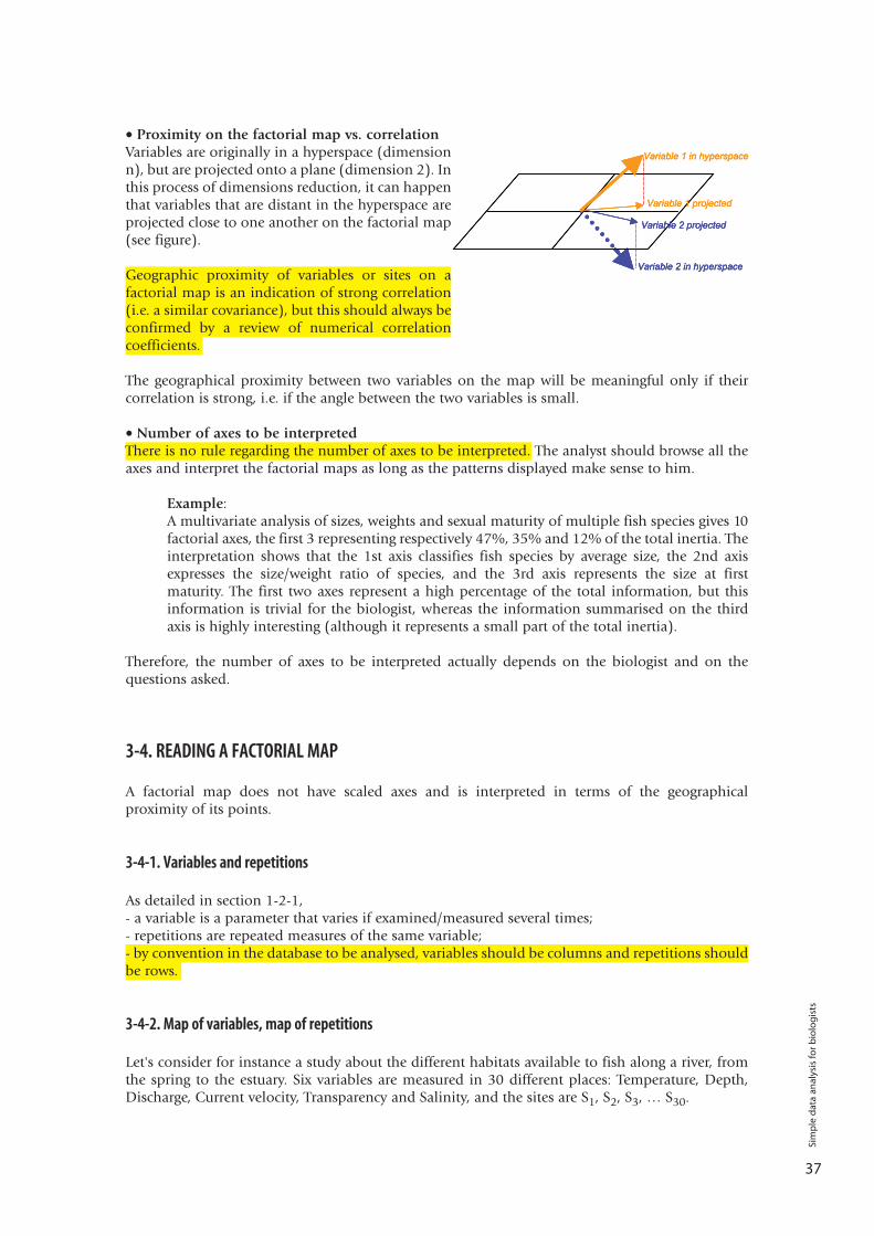
• Number of axes to be interpretedThere is no rule regarding the number of axes to be interpreted. The analyst should browse all theaxes and interpret the factorial maps as long as the patterns displayed make sense to him.

Example:A multivariate analysis of sizes, weights and sexual maturity of multiple fish species gives 10factorial axes, the first 3 representing respectively 47%, 35% and 12% of the total inertia. Theinterpretation shows that the 1st axis classifies fish species by average size, the 2nd axisexpresses the size/weight ratio of species, and the 3rd axis represents the size at firstmaturity. The first two axes represent a high percentage of the total information, but thisinformation is trivial for the biologist, whereas the information summarised on the thirdaxis is highly interesting (although it represents a small part of the total inertia).

Therefore, the number of axes to be interpreted actually depends on the biologist and on thequestions asked.

3-4. READING A FACTORIAL MAP

A factorial map does not have scaled axes and is interpreted in terms of the geographicalproximity of its points.

3-4-1. Variables and repetitions

As detailed in section 1-2-1,- a variable is a parameter that varies if examined/measured several times;- repetitions are repeated measures of the same variable;- by convention in the database to be analysed, variables should be columns and repetitions shouldbe rows.

3-4-2. Map of variables, map of repetitions

Let's consider for instance a study about the different habitats available to fish along a river, fromthe spring to the estuary. Six variables are measured in 30 different places: Temperature, Depth,Discharge, Current velocity, Transparency and Salinity, and the sites are S1, S2, S3, … S30.

37

Sim

ple

dat

a an

alys

is fo

r b

iolo

gis

ts

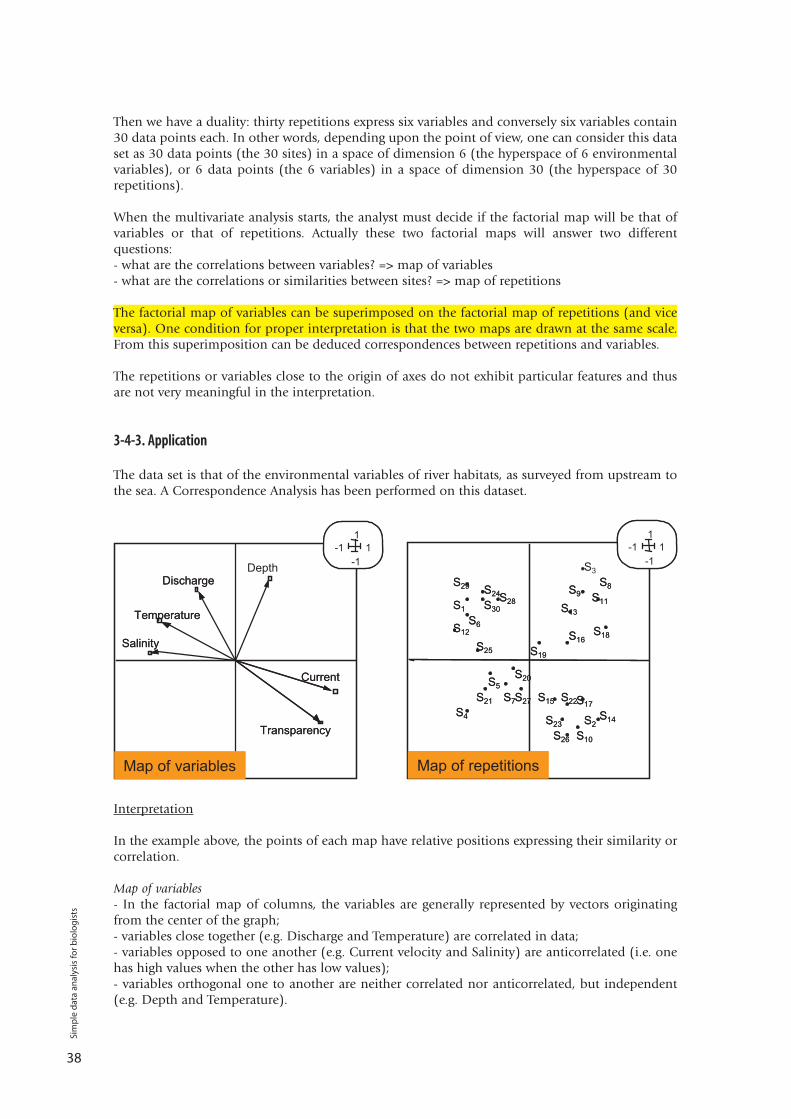
Then we have a duality: thirty repetitions express six variables and conversely six variables contain30 data points each. In other words, depending upon the point of view, one can consider this dataset as 30 data points (the 30 sites) in a space of dimension 6 (the hyperspace of 6 environmentalvariables), or 6 data points (the 6 variables) in a space of dimension 30 (the hyperspace of 30repetitions).

When the multivariate analysis starts, the analyst must decide if the factorial map will be that ofvariables or that of repetitions. Actually these two factorial maps will answer two differentquestions:- what are the correlations between variables? => map of variables- what are the correlations or similarities between sites? => map of repetitions

The factorial map of variables can be superimposed on the factorial map of repetitions (and viceversa). One condition for proper interpretation is that the two maps are drawn at the same scale.From this superimposition can be deduced correspondences between repetitions and variables.

The repetitions or variables close to the origin of axes do not exhibit particular features and thusare not very meaningful in the interpretation.

3-4-3. Application

The data set is that of the environmental variables of river habitats, as surveyed from upstream tothe sea. A Correspondence Analysis has been performed on this dataset.

Interpretation

In the example above, the points of each map have relative positions expressing their similarity orcorrelation.

Map of variables- In the factorial map of columns, the variables are generally represented by vectors originatingfrom the center of the graph;- variables close together (e.g. Discharge and Temperature) are correlated in data;- variables opposed to one another (e.g. Current velocity and Salinity) are anticorrelated (i.e. onehas high values when the other has low values);- variables orthogonal one to another are neither correlated nor anticorrelated, but independent(e.g. Depth and Temperature).

38

Sim

ple

dat

a an

alys

is fo

r b

iolo

gis

ts

Map of repetitions- Sites close together in a particular area of the map are similar in terms of variables measured (e.g.sites S1, S29, S24 have similar values of Temperature and Discharge);- sites opposed one to another on the factorial map have opposed values for their variables (e.g.high values of Temperature and Discharge in sites S1 or S29 but low values in sites S10 or S14);- sites located on a direction orthogonal to others do not have correlated variables (e.g. sites S11, S3,S8 do not have common features with sites S14, S2 or S10).

Global interpretationData actually reflect the evolution of habitats along the river. Sites located upstream, in themountains, have high current speed, high transparency (clear water), as well as low temperatureand low discharge; this defines a typical small mountain stream. Conversely, sites located by thesea, in the estuary, have higher salinity values, higher temperatures, and bigger discharge. Deeppools can also be found along the river, and then the depth is not correlated to any other variable.

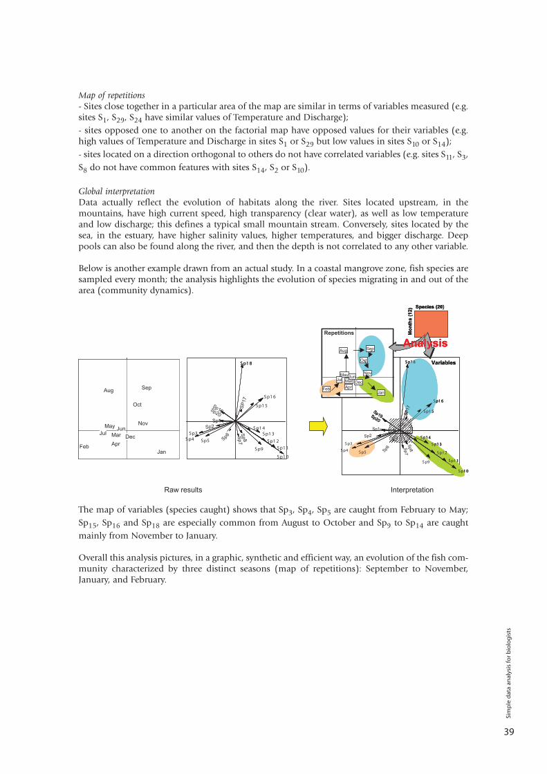
Below is another example drawn from an actual study. In a coastal mangrove zone, fish species aresampled every month; the analysis highlights the evolution of species migrating in and out of thearea (community dynamics).

The map of variables (species caught) shows that Sp3, Sp4, Sp5 are caught from February to May;Sp15, Sp16 and Sp18 are especially common from August to October and Sp9 to Sp14 are caughtmainly from November to January.

Overall this analysis pictures, in a graphic, synthetic and efficient way, an evolution of the fish com-munity characterized by three distinct seasons (map of repetitions): September to November,January, and February.

39

Sim

ple

dat

a an

alys

is fo

r b

iolo

gis

ts

3-5. PRE-ANALYSIS DATA PROCESSING

3-5-1. Centering

Centering a dataset consists of substracting a value from each cell; this value is calculated from ablock of rows or columns.

There are three types of centering: Centering by columnThis corresponds to deducing from each cell of a table the average value of the column to which itbelongs. In a table where columns are variables, centering by column corresponds to deducingfrom each value of the variable the mean of this variable.

Centering by rowThis corresponds to deducing from each cell of a table the average value of the row it belongs to. Ifrows consist of repetitions, then centering by row corresponds to deducing from each repetition themean of the values measured for this point.

Centering by blockThis corresponds to deducing from each cell of a block of values the average value of the block itbelongs to. For instance, in the case of a table of 50 rows corresponding to measures made in 5different locations (10 measures in site S1, 10 in site S2, etc.), centering by block corresponds toremoving from each cell of a block (= of a site) the average of measures in this site.

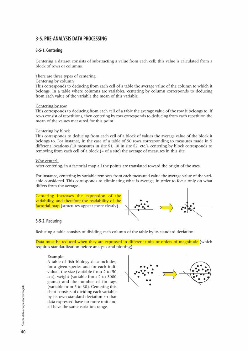
Why center? After centering, in a factorial map all the points are translated toward the origin of the axes.

For instance, centering by variable removes from each measured value the average value of the vari-able considered. This corresponds to eliminating what is average, in order to focus only on whatdiffers from the average.

Centering increases the expression of thevariability, and therefore the readability of thefactorial map (structures appear more clearly).

3-5-2. Reducing

Reducing a table consists of dividing each column of the table by its standard deviation.

Data must be reduced when they are expressed in different units or orders of magnitude (whichrequires standardization before analysis and plotting).

Example:A table of fish biology data includes,for a given species and for each indi-vidual, the size (variable from 2 to 50cm), weight (variable from 2 to 3000grams) and the number of fin rays(variable from 5 to 30). Centering thischart consists of dividing each variableby its own standard deviation so thatdata expressed have no more unit andall have the same variation range.

40

Sim

ple

dat

a an

alys

is fo

r b

iolo

gis

ts

3-5-3. Normalizing

Normalizing consists of centering and reducing data.

Equivalences:Centering + Reducing = NormalizingNormalizing = Standardizing

The reasons for normalizing are the sameas those for centering and reducing, i.e.respectively removing the mean to betterexpress specific patterns and homogenizingdata expressed in different units.

In a multivariate analysis, after normaliza-tion, the factorial axes will be expressed asa unit (+1) and the factorial map can berepresented as a circle.

3-6. MAIN TYPES OF ANALYSES

The various methods of multivariate analyses are classified into 3 broad categories: one-, two-, andK-tables analyses:- one-table analyses: one dataset is analysed (e.g. analysis of fish species caught at one site);- two-table analyses: two datasets are simultaneously analysed and compared (e.g. one table ofenvironmental variables and one table of fish data measured at one site);- K-table analyses: more than 2 datasets are simultaneously analysed and compared (e.g. tables offish species and of environmental variables measured at 3 different sites during 5 successive years(2 tables x 3 sites x 5 years = 30 tables).

Of course these analyses are of increasing complexity, and some methods developed to addressK-tables are quite recent and are not yet widely disseminated. They are just mentioned here forinformation.

3-6-1. One-table analyses (PCA, COA and others)

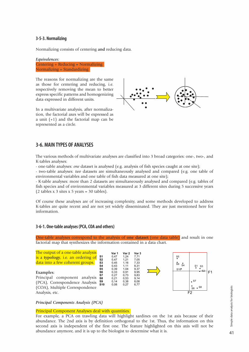
One-table analyses correspond to the analysis of one dataset (one data table) and result in onefactorial map that synthesizes the information contained in a data chart.

The output of a one-table analysisis a typology, i.e. an ordering ofdata into a few coherent groups.

Examples:Principal component analysis(PCA), Correspondence Analysis(COA), Multiple CorrespondenceAnalysis, etc.

Principal Components Analysis (PCA)

Principal Component Analyses deal with quantities.For example, a PCA on trawling data will highlight sardines on the 1st axis because of theirabundance. The 2nd axis is by definition orthogonal to the 1st. Thus, the information on thissecond axis is independent of the first one. The feature highlighted on this axis will not beabundance anymore, and it is up to the biologist to determine what it is. 41

Sim

ple

dat

a an

alys

is fo

r b

iolo

gis

ts

Thus, in a multivariate analysis of sizes, weights and sexual maturity of multiple fish species, axisF1 might classify fish species by average size, then F2 classify species according to their size/weightratio, and F3 order species according to their size at first maturity.

There are 2 fundamental types of PCAs: - covariance matrix PCAs, on centered but non-reduced data

for analyses of variables expressed in the same unit (e.g. abundance of each species)- correlation matrix PCAs, on standardized (=centered + reduced) data

for analyses of variables of different units (e.g. temperature, salinity, etc.)

Correspondence Analysis (COA)

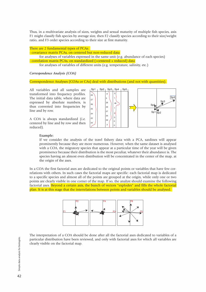
Correspondence Analyses (COAs or CAs) deal with distributions (and not with quantities).

All variables and all samples aretransformed into frequency profiles.The initial data table, where data areexpressed by absolute numbers, isthus converted into frequencies byline and by row.

A COA is always standardized (i.e.centered by line and by row and thenreduced).

Example:If we consider the analysis of the trawl fishery data with a PCA, sardines will appearprominently because they are more numerous. However, when the same dataset is analysedwith a COA, the migratory species that appear at a particular time of the year will be givenprominence because their distribution is the most peculiar, whatever their abundance is. Thespecies having an almost even distribution will be concentrated in the center of the map, atthe origin of the axes.

In a COA the first factorial axes are dedicated to the original points or variables that have few cor-relations with others. In such cases the factorial maps are specific: each factorial map is dedicatedto a specific species and almost all of the points are grouped at the origin, while only one or twopoints are clearly visible in one corner of the map. If so, the analyst should examine the followingfactorial axes. Beyond a certain axis, the bunch of vectors "explodes" and fills the whole factorialplan. It is at this stage that the interrelations between points and variables should be analysed.

The interpretation of a COA should be done after all the factorial axes dedicated to variables of aparticular distribution have been reviewed, and only with factorial axes for which all variables areclearly visible on the factorial map.

42

Sim

ple

dat

a an

alys

is fo

r b

iolo

gis

ts

There are two doctrines for the interpretation of a COA. The ancient school holds that:- some original but trivial rows or columns "disrupt" the analysis; once noticed they are removedfrom the data table, and the analysis is run again on the remaining data; - the explained variance expressed by axes F1 and F2 (after removal of "trivial" variables orrepetitions) illustrates the quality of the summary interpreted.The recent school holds instead that: - removing data introduces unwelcome biases and should not be done;- the first axes, containing an important part of the total inertia, are dedicated to specificities andare of little interest in exploratory terms. On the other hand, at the level of axes that better expressrelationships between variables, the explained variance is low. This is not a problem and the per-centage of inertia expressed by those two axes is not integrated into the interpretation.

Multiple Correspondence Analysis (MCA)

The multiple correspondence analysis is the equivalent of a correspondence analysis performed ona data table in which variables are discontinuous (i.e. expressed in the form of categories).

The calculation is almost the same as for a COA; the only difference is that the software transforms("discretizes") the initial discontinuous variables into as many variables as there are categoriesoverall, before processing them like a COA. These discretized variables will then be analyzed andthen interpreted like a standard COA.

Example:Analysis of the results of a poll on personal tastes. Question: Do you like beef/chicken/pork/fish?Answer: not at all/a little/a lot Repetitions are persons. For each food type, the answer of a person falls into 3 possiblecategories. The analysis software will transform these categories into disjunctive variables(Not at all: yes/no; A little: yes/no; A lot: yes/no).

3-6-2. Two-table and K-table analyses

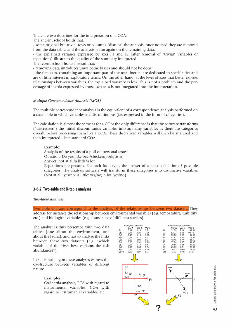
Two-table analyses

Two-table analyses correspond to the analysis of the relationships between two datasets. Theyaddress for instance the relationship between environmental variables (e.g. temperature, turbidity,etc.) and biological variables (e.g. abundance of different species).

The analyst is thus presented with two datatables (one about the environment, oneabout the fauna), and has to analyse the linksbetween these two datasets (e.g. "whichvariable of the river best explains the fishabundance?").

In statistical jargon these analyses express theco-structure between variables of differentnature.

Examples:Co-inertia analysis, PCA with regard toinstrumental variables, COA withregard to instrumental variables, etc.

43

Sim

ple

dat

a an

alys

is fo

r b

iolo

gis

ts

K-table analyses

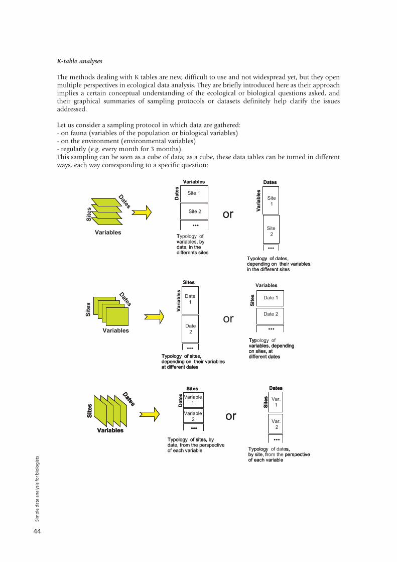
The methods dealing with K tables are new, difficult to use and not widespread yet, but they openmultiple perspectives in ecological data analysis. They are briefly introduced here as their approachimplies a certain conceptual understanding of the ecological or biological questions asked, andtheir graphical summaries of sampling protocols or datasets definitely help clarify the issuesaddressed.

Let us consider a sampling protocol in which data are gathered:- on fauna (variables of the population or biological variables) - on the environment (environmental variables) - regularly (e.g. every month for 3 months).This sampling can be seen as a cube of data; as a cube, these data tables can be turned in differentways, each way corresponding to a specific question:

44

Sim

ple

dat

a an

alys

is fo

r b

iolo

gis

ts

45

Sim

ple

dat

a an

alys

is fo

r b

iolo

gis

ts

4-1. DEFINITIONS AND PRINCIPLES

4-1-1. Mean, median, variance

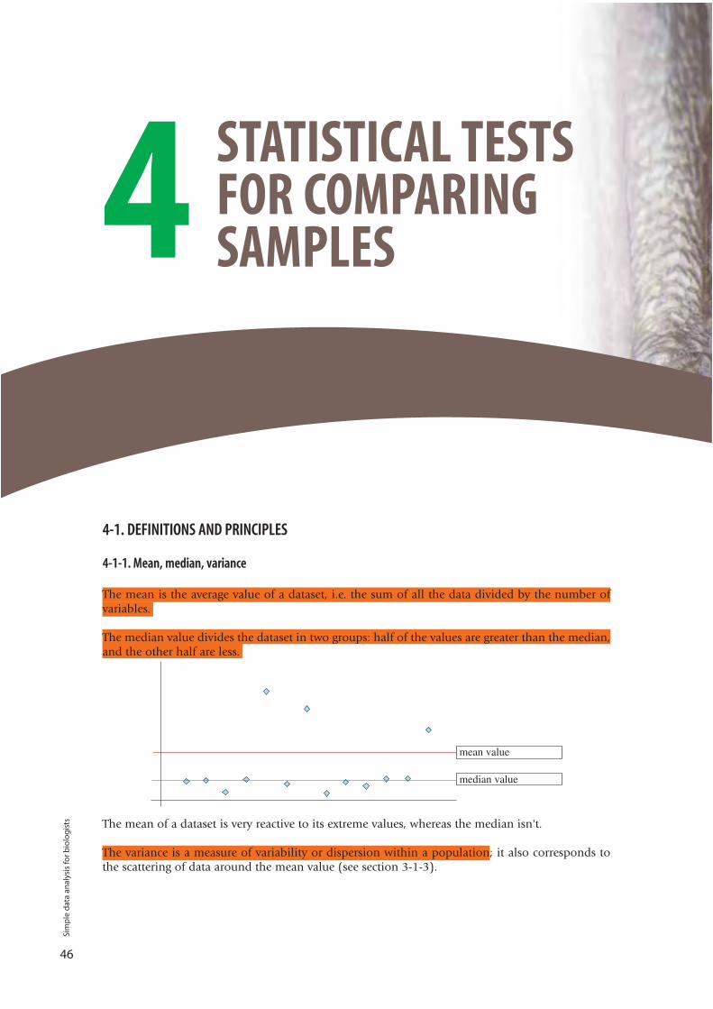
The mean is the average value of a dataset, i.e. the sum of all the data divided by the number ofvariables.

The median value divides the dataset in two groups: half of the values are greater than the median,and the other half are less.

The mean of a dataset is very reactive to its extreme values, whereas the median isn't.

The variance is a measure of variability or dispersion within a population; it also corresponds tothe scattering of data around the mean value (see section 3-1-3).

4 STATISTICAL TESTSFOR COMPARINGSAMPLES

46

Sim

ple

dat

a an

alys

is fo

r b

iolo

gis

ts

4-1-2. Normal distribution

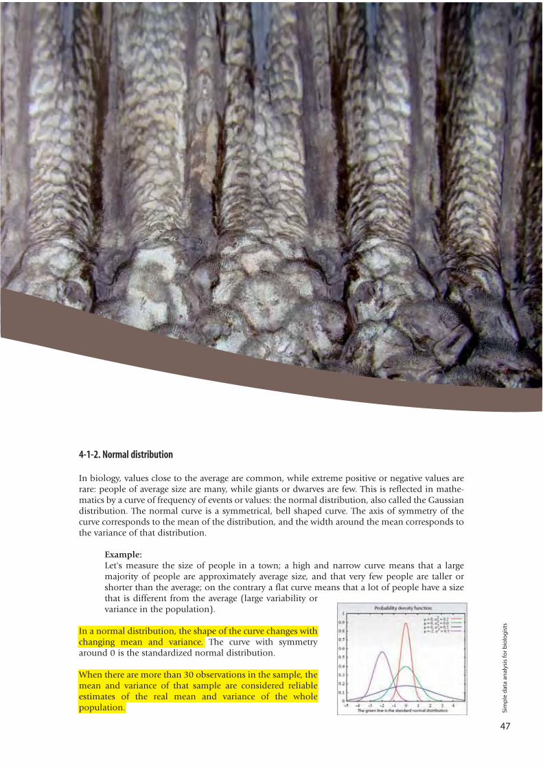
In biology, values close to the average are common, while extreme positive or negative values arerare: people of average size are many, while giants or dwarves are few. This is reflected in mathe-matics by a curve of frequency of events or values: the normal distribution, also called the Gaussiandistribution. The normal curve is a symmetrical, bell shaped curve. The axis of symmetry of thecurve corresponds to the mean of the distribution, and the width around the mean corresponds tothe variance of that distribution.

Example:Let's measure the size of people in a town; a high and narrow curve means that a largemajority of people are approximately average size, and that very few people are taller orshorter than the average; on the contrary a flat curve means that a lot of people have a sizethat is different from the average (large variability orvariance in the population).

In a normal distribution, the shape of the curve changes withchanging mean and variance. The curve with symmetryaround 0 is the standardized normal distribution.

When there are more than 30 observations in the sample, themean and variance of that sample are considered reliableestimates of the real mean and variance of the wholepopulation.

47

Sim

ple

dat

a an

alys

is fo

r b

iolo

gis

ts

4-1-3. Questions and hypotheses

A hypothesis is a predictive statement that is tested by investigation, and investigation may provideevidence to support or reject the hypothesis.

From a statistical viewpoint, a biological question has to be phrased as an experimentalhypothesis, which creates in turn a null hypothesis. The null hypothesis is the opposite of thehypothesis; the hypothesis typically assumes that there is a difference between samples, whereasthe null hypothesis typically assumes that there is no difference between samples ("nullhypothesis = difference is nil")

Biological question: is the density of fish in the flooded forest different to the density of fish in theriver mainstream? Experimental hypothesis: the density of fish in flooded forest habitats is different to the density offish in rivers.Null hypothesis: there is no difference between the density of fish in flooded forests and in rivers(in other words, the mean density of fish in flooded forests equals the mean density of fish inrivers).

To decide whether to accept or reject the null hypothesis a statistical test must be run. Statistical tests test the null hypothesis.

The statistical test produces a probability value that indicates the probability of obtaining oursample values if the null hypothesis is true. If this probability value is less than a pre-determined critical threshold (or significance level) thenthe null hypothesis is rejected.

4-1-4. Probability and significance

In most statistical analyses uncertainty is thought of in terms of probabilities. Probability is usual-ly viewed in terms of events; the probability of event A occurring is written P(A). Probabilities canbe between 0 and 1. When P(A) = 0 then the event is impossible; when P(A) = 1 then the event iscertain.

A statistical test is performed to determine the probability that two samples have come from thesame statistical population (i.e. to determine if the two samples are the same or different). The testswill produce a P value which is the probability of obtaining our sample values (or ones moreextreme) if the null hypothesis is true, i.e. if our samples come from the same population.

If the calculated P value is below a critical threshold, the samples are said to be significantlydifferent.

If a test produces a probability value that is equal to or less than a certain arbitrary threshold, theresult is said to be statistically significant, i.e. the probability of the tested event occurring is lessthan the scientist is willing to accept.

While significance levels are arbitrary, they are conventionally set at α = 0.05 (i.e. 1 in 20) andα = 0.01 (i.e. 1 in 100). Whichever significance level is adopted, it must be set before the statisticaltest is run i.e. it must be set a priori.

Example:A fisheries scientist wants to determine if catfish in the Tonle Sap Lake are larger or smallerthan catfish in the Mekong River.• Question: Is the size of Tonle Sap catfish different from the size of Mekong River catfish? • Hypothesis: Catfish in the Tonle Sap Lake will be a different size to those in the MekongRiver.• Null Hypothesis: Catfish in the Tonle Sap Lake will be the same size as those in the MekongRiver48

Sim

ple

dat

a an

alys

is fo

r b

iolo

gis

ts

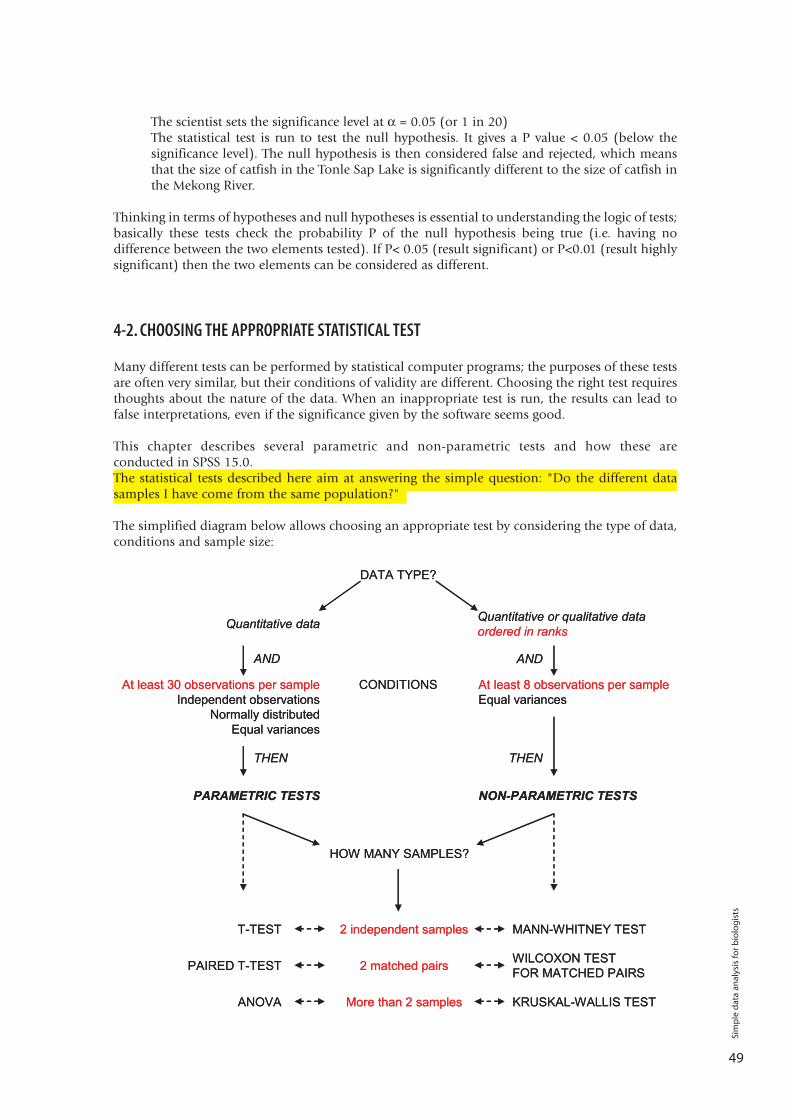
49

The scientist sets the significance level at α = 0.05 (or 1 in 20)The statistical test is run to test the null hypothesis. It gives a P value < 0.05 (below thesignificance level). The null hypothesis is then considered false and rejected, which meansthat the size of catfish in the Tonle Sap Lake is significantly different to the size of catfish inthe Mekong River.

Thinking in terms of hypotheses and null hypotheses is essential to understanding the logic of tests;basically these tests check the probability P of the null hypothesis being true (i.e. having nodifference between the two elements tested). If P< 0.05 (result significant) or P<0.01 (result highlysignificant) then the two elements can be considered as different.

4-2. CHOOSING THE APPROPRIATE STATISTICAL TEST

Many different tests can be performed by statistical computer programs; the purposes of these testsare often very similar, but their conditions of validity are different. Choosing the right test requiresthoughts about the nature of the data. When an inappropriate test is run, the results can lead tofalse interpretations, even if the significance given by the software seems good.

This chapter describes several parametric and non-parametric tests and how these areconducted in SPSS 15.0.The statistical tests described here aim at answering the simple question: "Do the different datasamples I have come from the same population?"

The simplified diagram below allows choosing an appropriate test by considering the type of data,conditions and sample size:

Sim

ple

dat

a an

alys

is fo

r b

iolo

gis

ts

50

4-2-1. Parametric versus non-parametric tests

Parametric tests allow testing hypotheses related to means. They use rigorous and often complexmathematical theory and require a probability distribution to be specified for the populations fromwhich samples were taken (this is usually the normal distribution).

Non-parametric tests use ranks of the observations to compare medians rather than means. Thisremoves the need for data to be normally distributed. Non-parametric tests are less powerful thanparametric tests, because they don't use the actual values of the observations, but only the ranks ofthe observations (thus, it is often said that they lose information).

Both parametric and non-parametric tests have assumptions about the data that must be met toensure that the test is reliable.

Conditions of parametric testsParametric tests have three assumptions that theoretically must be met in order for the outcomesof the tests to be reliable. The assumptions of parametric tests are as follows:

1. The samples come from normally distributed populations. However, parametric tests are usually fairly robust to moderate violations of this assumption providing the sample sizes of the samples to be compared are equal. Transformation of the variable to a different scale can also improve its normality (see section 4-2-2.).

2. The samples come from populations with equal variances. This assumption is more critical than that of normality but again tests are reasonably robust if sample sizes are equal. In addition, variances are often unequal because distributions are skewed. Therefore fixing issues of non-normality through transformation will often makevariances more similar.

3. The observations should be independent of each other, both within and betweensample groups. This assumption must be considered in the design phase of the study.

The presence of outliers (extreme values that are very different from the rest) often have strongeffects on the outcomes of the tests. Both parametric and non-parametric tests are influenced by thepresence of outliers; but non-parametric tests are less sensitive to outliers.

Conditions of non-parametric testsWhile there are fewer conditions required to run non-parametric tests, some should still be met toensure the reliability of the tests. The assumptions of non-parametric tests are as follows:

1. The samples must have equal variances.2. Distributions of the populations must be similar (but they do not have to follow the

normal distribution).

One of the big advantages of non-parametric tests is that they do not require data to be normallydistributed. Non-parametric tests are recommended over parametric tests when (i) distributions arevery strange and not improved by transformation and/or (ii) outliers are present.

4-2-2. Transformations

Transformations are performed on raw observation values in order to help data meet theassumptions of particular statistical tests; specifically: (i) to make the data closer to a normaldistribution; (ii) to help variances become more equal and; (iii) to reduce the influence of outliers.Because of these things, running statistical tests on transformed data will often make the tests morereliable; however, whether the data meets the assumptions of the tests should always be re-checkedafter transformation. Data transformation is not considered fiddling with data or cheating becausemany scales of measurement are arbitrary. However, a decision to transform data must always bemade before the analysis is done!

Sim

ple

dat

a an

alys

is fo

r b

iolo

gis

ts

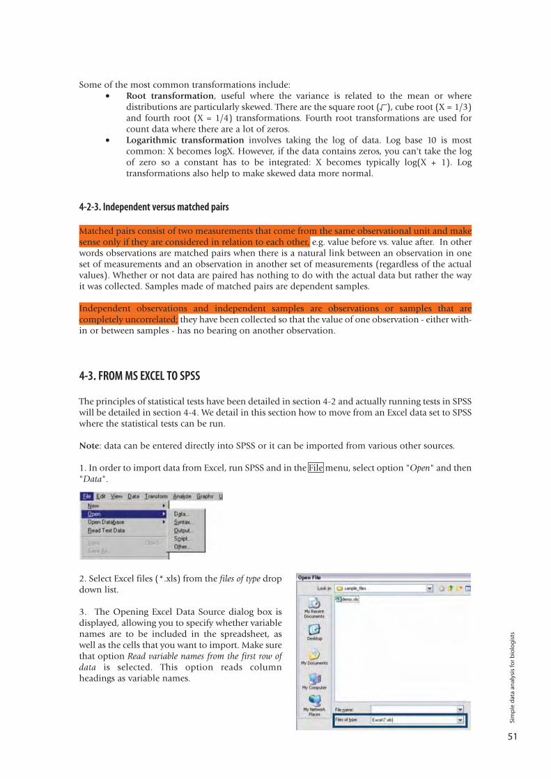
51

Some of the most common transformations include:• Root transformation, useful where the variance is related to the mean or where

distributions are particularly skewed. There are the square root ( ), cube root (X = 1/3) and fourth root (X = 1/4) transformations. Fourth root transformations are used for count data where there are a lot of zeros.

• Logarithmic transformation involves taking the log of data. Log base 10 is most common: X becomes logX. However, if the data contains zeros, you can't take the log of zero so a constant has to be integrated: X becomes typically log(X + 1). Log transformations also help to make skewed data more normal.

4-2-3. Independent versus matched pairs

Matched pairs consist of two measurements that come from the same observational unit and makesense only if they are considered in relation to each other, e.g. value before vs. value after. In otherwords observations are matched pairs when there is a natural link between an observation in oneset of measurements and an observation in another set of measurements (regardless of the actualvalues). Whether or not data are paired has nothing to do with the actual data but rather the wayit was collected. Samples made of matched pairs are dependent samples.

Independent observations and independent samples are observations or samples that arecompletely uncorrelated; they have been collected so that the value of one observation - either with-in or between samples - has no bearing on another observation.

4-3. FROM MS EXCEL TO SPSS

The principles of statistical tests have been detailed in section 4-2 and actually running tests in SPSSwill be detailed in section 4-4. We detail in this section how to move from an Excel data set to SPSSwhere the statistical tests can be run.

Note: data can be entered directly into SPSS or it can be imported from various other sources.

1. In order to import data from Excel, run SPSS and in the File menu, select option "Open" and then"Data".

2. Select Excel files (*.xls) from the files of type dropdown list.

3. The Opening Excel Data Source dialog box isdisplayed, allowing you to specify whether variablenames are to be included in the spreadsheet, aswell as the cells that you want to import. Make surethat option Read variable names from the first row ofdata is selected. This option reads columnheadings as variable names.

Sim

ple

dat

a an

alys

is fo

r b

iolo

gis

ts

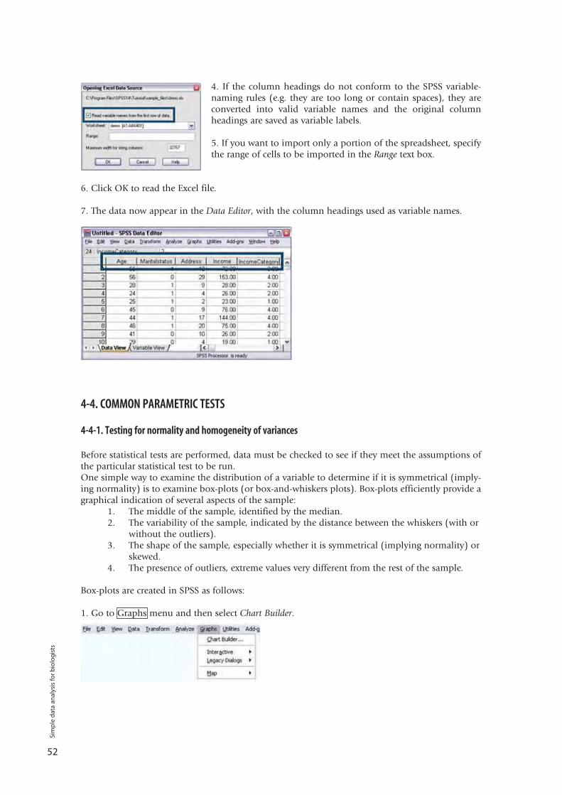
52

4. If the column headings do not conform to the SPSS variable-naming rules (e.g. they are too long or contain spaces), they areconverted into valid variable names and the original columnheadings are saved as variable labels.

5. If you want to import only a portion of the spreadsheet, specifythe range of cells to be imported in the Range text box.

6. Click OK to read the Excel file.

7. The data now appear in the Data Editor, with the column headings used as variable names.

4-4. COMMON PARAMETRIC TESTS

4-4-1. Testing for normality and homogeneity of variances

Before statistical tests are performed, data must be checked to see if they meet the assumptions ofthe particular statistical test to be run. One simple way to examine the distribution of a variable to determine if it is symmetrical (imply-ing normality) is to examine box-plots (or box-and-whiskers plots). Box-plots efficiently provide agraphical indication of several aspects of the sample:

1. The middle of the sample, identified by the median.2. The variability of the sample, indicated by the distance between the whiskers (with or

without the outliers).3. The shape of the sample, especially whether it is symmetrical (implying normality) or

skewed.4. The presence of outliers, extreme values very different from the rest of the sample.

Box-plots are created in SPSS as follows:

1. Go to Graphs menu and then select Chart Builder.

Sim

ple

dat

a an

alys

is fo

r b

iolo

gis

ts

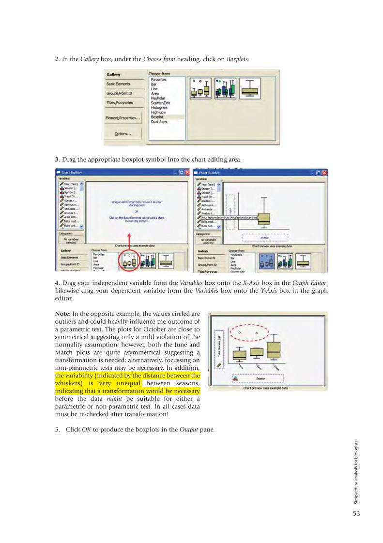
53

2. In the Gallery box, under the Choose from heading, click on Boxplots.

3. Drag the appropriate boxplot symbol into the chart editing area.

4. Drag your independent variable from the Variables box onto the X-Axis box in the Graph Editor.Likewise drag your dependent variable from the Variables box onto the Y-Axis box in the grapheditor.

Note: In the opposite example, the values circled areoutliers and could heavily influence the outcome ofa parametric test. The plots for October are close tosymmetrical suggesting only a mild violation of thenormality assumption; however, both the June andMarch plots are quite asymmetrical suggesting atransformation is needed; alternatively, focussing onnon-parametric tests may be necessary. In addition,the variability (indicated by the distance between thewhiskers) is very unequal between seasons,indicating that a transformation would be necessarybefore the data might be suitable for either aparametric or non-parametric test. In all cases datamust be re-checked after transformation!

5. Click OK to produce the boxplots in the Output pane.

Sim

ple

dat

a an

alys

is fo

r b

iolo

gis

ts

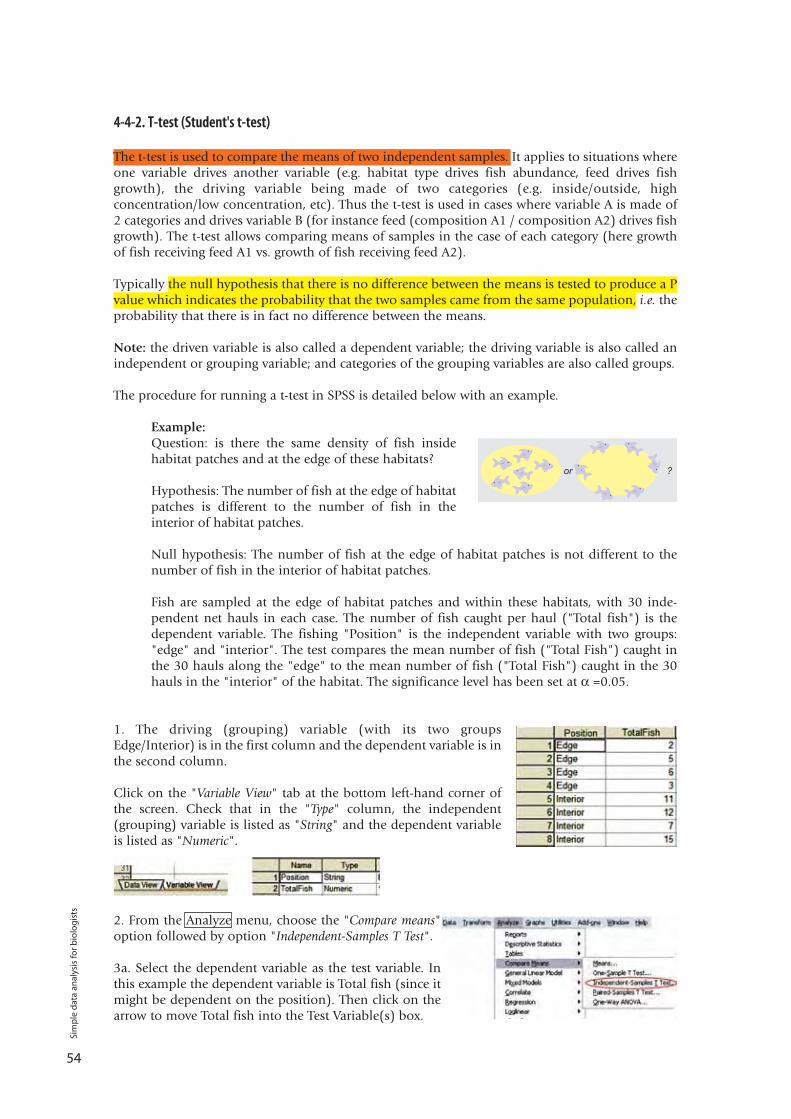
54

4-4-2. T-test (Student's t-test)

The t-test is used to compare the means of two independent samples. It applies to situations whereone variable drives another variable (e.g. habitat type drives fish abundance, feed drives fishgrowth), the driving variable being made of two categories (e.g. inside/outside, highconcentration/low concentration, etc). Thus the t-test is used in cases where variable A is made of2 categories and drives variable B (for instance feed (composition A1 / composition A2) drives fishgrowth). The t-test allows comparing means of samples in the case of each category (here growthof fish receiving feed A1 vs. growth of fish receiving feed A2).

Typically the null hypothesis that there is no difference between the means is tested to produce a Pvalue which indicates the probability that the two samples came from the same population, i.e. theprobability that there is in fact no difference between the means.

Note: the driven variable is also called a dependent variable; the driving variable is also called anindependent or grouping variable; and categories of the grouping variables are also called groups.

The procedure for running a t-test in SPSS is detailed below with an example.

Example:Question: is there the same density of fish insidehabitat patches and at the edge of these habitats?

Hypothesis: The number of fish at the edge of habitatpatches is different to the number of fish in theinterior of habitat patches.

Null hypothesis: The number of fish at the edge of habitat patches is not different to thenumber of fish in the interior of habitat patches.

Fish are sampled at the edge of habitat patches and within these habitats, with 30 inde-pendent net hauls in each case. The number of fish caught per haul ("Total fish") is thedependent variable. The fishing "Position" is the independent variable with two groups:"edge" and "interior". The test compares the mean number of fish ("Total Fish") caught inthe 30 hauls along the "edge" to the mean number of fish ("Total Fish") caught in the 30hauls in the "interior" of the habitat. The significance level has been set at α =0.05.

1. The driving (grouping) variable (with its two groupsEdge/Interior) is in the first column and the dependent variable is inthe second column.

Click on the "Variable View" tab at the bottom left-hand corner ofthe screen. Check that in the "Type" column, the independent(grouping) variable is listed as "String" and the dependent variableis listed as "Numeric".

2. From the Analyze menu, choose the "Compare means"option followed by option "Independent-Samples T Test".

3a. Select the dependent variable as the test variable. Inthis example the dependent variable is Total fish (since itmight be dependent on the position). Then click on thearrow to move Total fish into the Test Variable(s) box.

Sim

ple

dat

a an

alys

is fo

r b

iolo

gis

ts

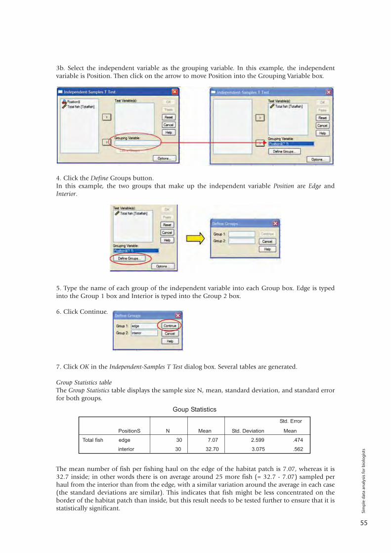
55

3b. Select the independent variable as the grouping variable. In this example, the independentvariable is Position. Then click on the arrow to move Position into the Grouping Variable box.

4. Click the Define Groups button.In this example, the two groups that make up the independent variable Position are Edge andInterior.

5. Type the name of each group of the independent variable into each Group box. Edge is typedinto the Group 1 box and Interior is typed into the Group 2 box.

6. Click Continue.

7. Click OK in the Independent-Samples T Test dialog box. Several tables are generated.

Group Statistics tableThe Group Statistics table displays the sample size N, mean, standard deviation, and standard errorfor both groups.

The mean number of fish per fishing haul on the edge of the habitat patch is 7.07, whereas it is32.7 inside; in other words there is on average around 25 more fish (= 32.7 - 7.07) sampled perhaul from the interior than from the edge, with a similar variation around the average in each case(the standard deviations are similar). This indicates that fish might be less concentrated on theborder of the habitat patch than inside, but this result needs to be tested further to ensure that it isstatistically significant.

Goup Statistics

Std. Error

PositionS N Mean Std. Deviation Mean

Total fish edge 30 7.07 2.599 .474

interior 30 32.70 3.075 .562

Sim

ple

dat

a an

alys

is fo

r b

iolo

gis

ts

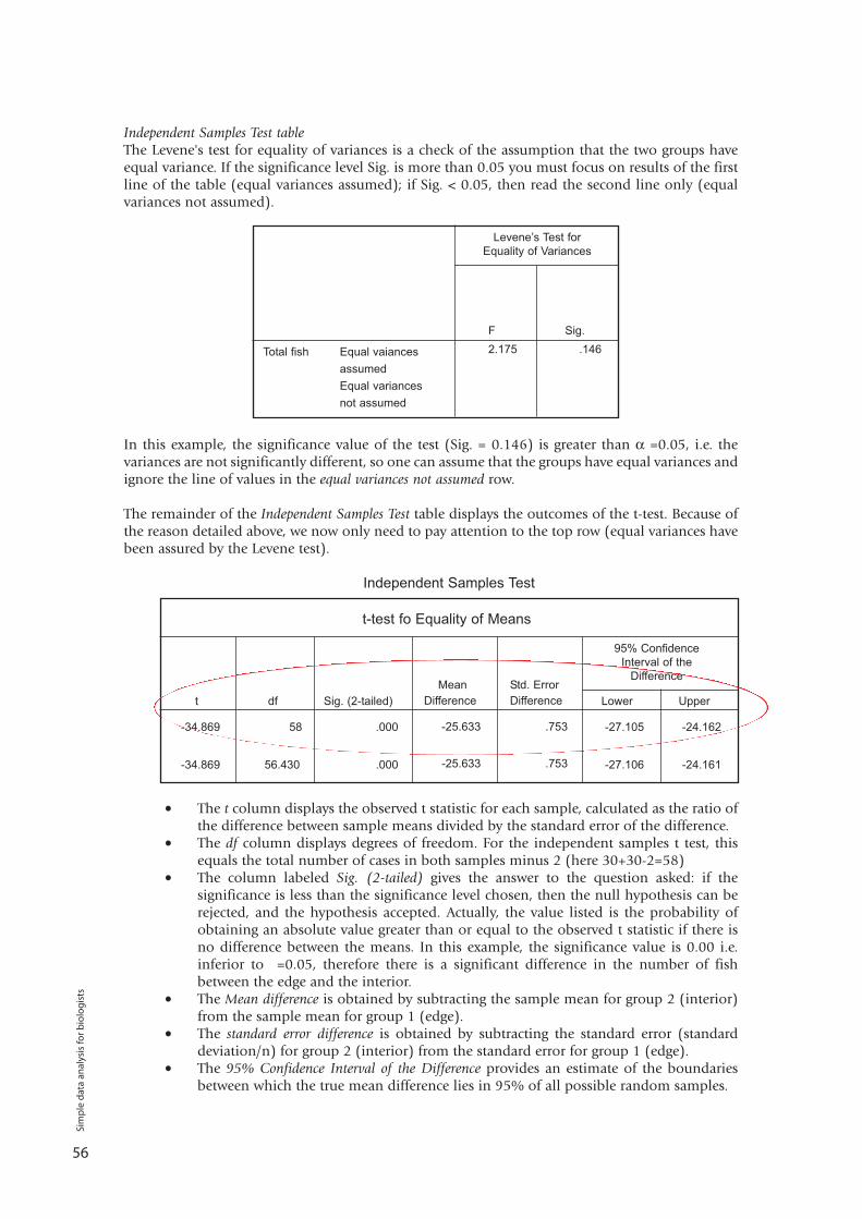
56

Independent Samples Test tableThe Levene's test for equality of variances is a check of the assumption that the two groups haveequal variance. If the significance level Sig. is more than 0.05 you must focus on results of the firstline of the table (equal variances assumed); if Sig. < 0.05, then read the second line only (equalvariances not assumed).

In this example, the significance value of the test (Sig. = 0.146) is greater than α =0.05, i.e. thevariances are not significantly different, so one can assume that the groups have equal variances andignore the line of values in the equal variances not assumed row.

The remainder of the Independent Samples Test table displays the outcomes of the t-test. Because ofthe reason detailed above, we now only need to pay attention to the top row (equal variances havebeen assured by the Levene test).

• The t column displays the observed t statistic for each sample, calculated as the ratio of the difference between sample means divided by the standard error of the difference.

• The df column displays degrees of freedom. For the independent samples t test, this equals the total number of cases in both samples minus 2 (here 30+30-2=58)

• The column labeled Sig. (2-tailed) gives the answer to the question asked: if the significance is less than the significance level chosen, then the null hypothesis can be rejected, and the hypothesis accepted. Actually, the value listed is the probability of obtaining an absolute value greater than or equal to the observed t statistic if there is no difference between the means. In this example, the significance value is 0.00 i.e. inferior to =0.05, therefore there is a significant difference in the number of fish between the edge and the interior.

• The Mean difference is obtained by subtracting the sample mean for group 2 (interior) from the sample mean for group 1 (edge).

• The standard error difference is obtained by subtracting the standard error (standard deviation/n) for group 2 (interior) from the standard error for group 1 (edge).

• The 95% Confidence Interval of the Difference provides an estimate of the boundaries between which the true mean difference lies in 95% of all possible random samples.

Levene’s Test forEquality of Variances

Total fish Equal vaiancesassumedEqual variancesnot assumed

F Sig.2.175 .146

Independent Samples Test

t-test fo Equality of Means

t

-34.869

-34.869

df

58

56.430

Sig. (2-tailed)

.000

.000

Lower

-27.105

-27.106

95% ConfidenceInterval of the

Difference

Upper

-24.162

-24.161

MeanDifference

-25.633

-25.633

Std. ErrorDifference

.753

.753

Sim

ple

dat

a an

alys

is fo

r b

iolo

gis

ts

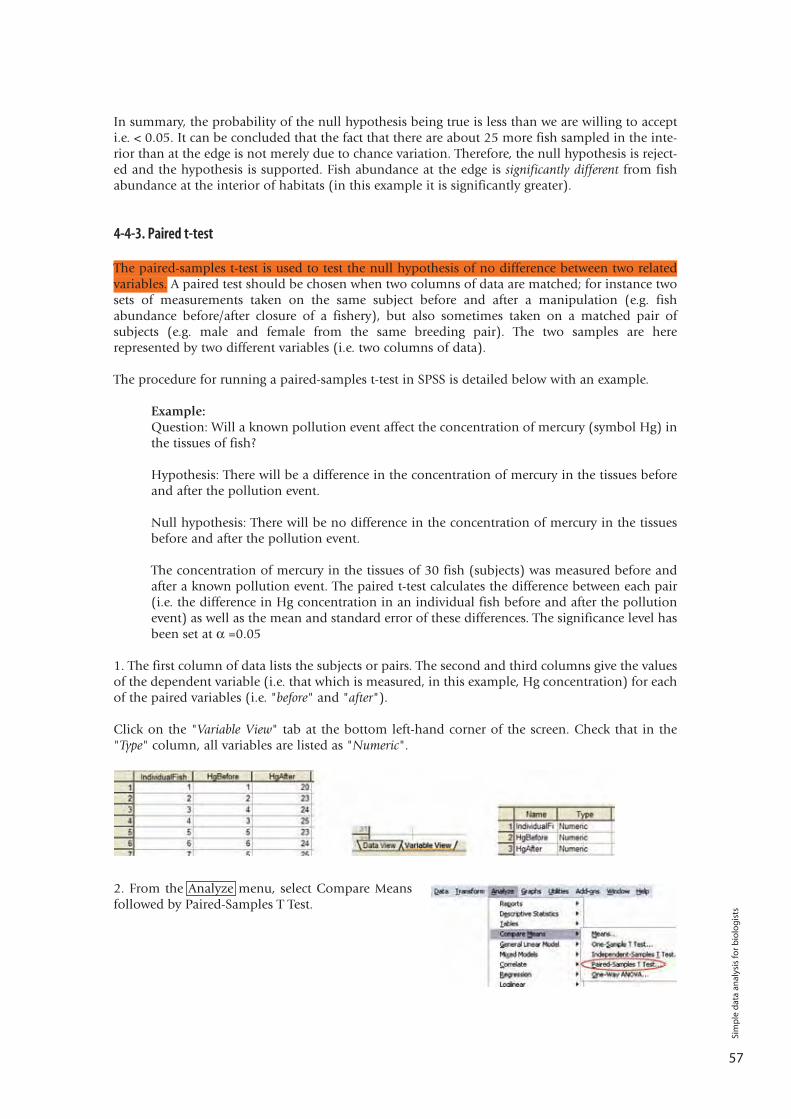
57

In summary, the probability of the null hypothesis being true is less than we are willing to accepti.e. < 0.05. It can be concluded that the fact that there are about 25 more fish sampled in the inte-rior than at the edge is not merely due to chance variation. Therefore, the null hypothesis is reject-ed and the hypothesis is supported. Fish abundance at the edge is significantly different from fishabundance at the interior of habitats (in this example it is significantly greater).

4-4-3. Paired t-test

The paired-samples t-test is used to test the null hypothesis of no difference between two relatedvariables. A paired test should be chosen when two columns of data are matched; for instance twosets of measurements taken on the same subject before and after a manipulation (e.g. fishabundance before/after closure of a fishery), but also sometimes taken on a matched pair ofsubjects (e.g. male and female from the same breeding pair). The two samples are hererepresented by two different variables (i.e. two columns of data).

The procedure for running a paired-samples t-test in SPSS is detailed below with an example.

Example:Question: Will a known pollution event affect the concentration of mercury (symbol Hg) inthe tissues of fish?

Hypothesis: There will be a difference in the concentration of mercury in the tissues beforeand after the pollution event.

Null hypothesis: There will be no difference in the concentration of mercury in the tissuesbefore and after the pollution event.

The concentration of mercury in the tissues of 30 fish (subjects) was measured before andafter a known pollution event. The paired t-test calculates the difference between each pair(i.e. the difference in Hg concentration in an individual fish before and after the pollutionevent) as well as the mean and standard error of these differences. The significance level hasbeen set at α =0.05

1. The first column of data lists the subjects or pairs. The second and third columns give the valuesof the dependent variable (i.e. that which is measured, in this example, Hg concentration) for eachof the paired variables (i.e. "before" and "after").

Click on the "Variable View" tab at the bottom left-hand corner of the screen. Check that in the"Type" column, all variables are listed as "Numeric".

2. From the Analyze menu, select Compare Meansfollowed by Paired-Samples T Test.

Sim

ple

dat

a an

alys

is fo

r b

iolo

gis

ts

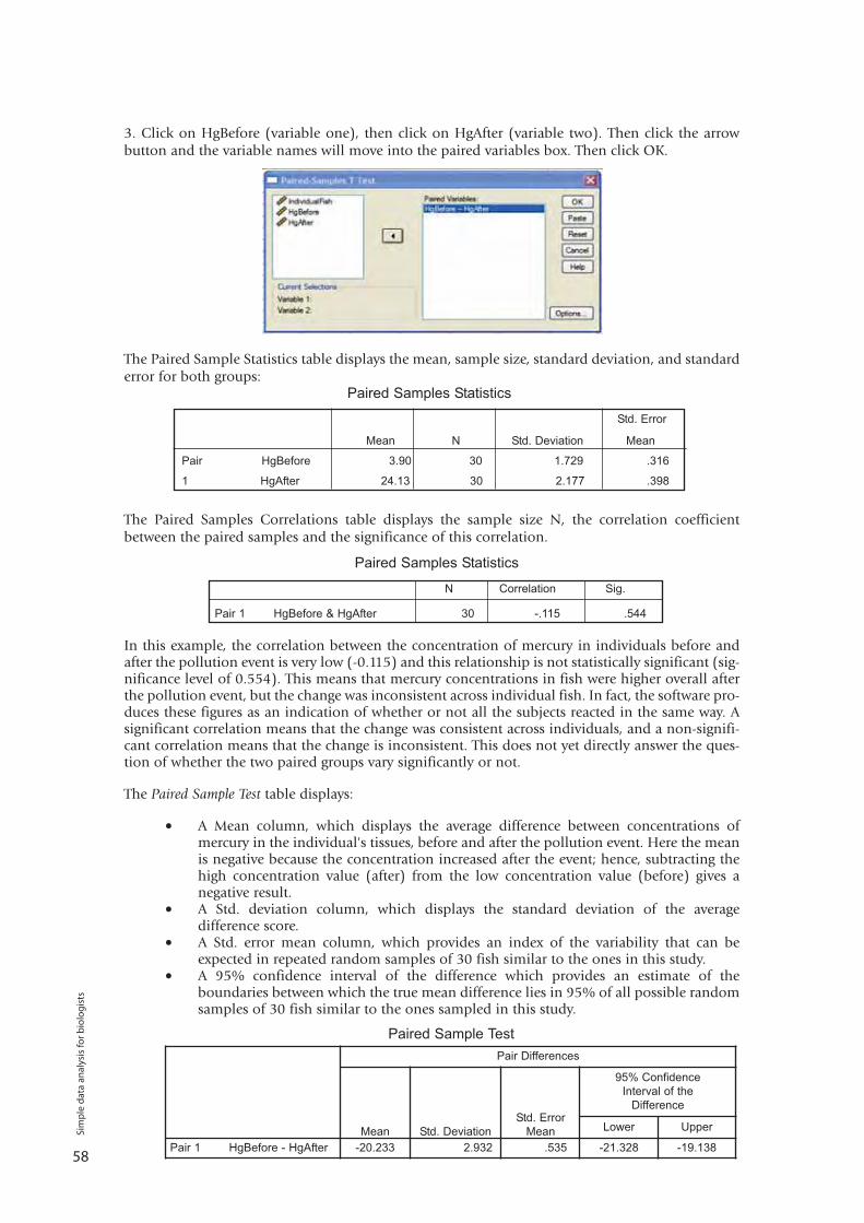
58

3. Click on HgBefore (variable one), then click on HgAfter (variable two). Then click the arrowbutton and the variable names will move into the paired variables box. Then click OK.

The Paired Sample Statistics table displays the mean, sample size, standard deviation, and standarderror for both groups:

The Paired Samples Correlations table displays the sample size N, the correlation coefficientbetween the paired samples and the significance of this correlation.

In this example, the correlation between the concentration of mercury in individuals before andafter the pollution event is very low (-0.115) and this relationship is not statistically significant (sig-nificance level of 0.554). This means that mercury concentrations in fish were higher overall afterthe pollution event, but the change was inconsistent across individual fish. In fact, the software pro-duces these figures as an indication of whether or not all the subjects reacted in the same way. Asignificant correlation means that the change was consistent across individuals, and a non-signifi-cant correlation means that the change is inconsistent. This does not yet directly answer the ques-tion of whether the two paired groups vary significantly or not.

The Paired Sample Test table displays:

• A Mean column, which displays the average difference between concentrations of mercury in the individual's tissues, before and after the pollution event. Here the mean is negative because the concentration increased after the event; hence, subtracting the high concentration value (after) from the low concentration value (before) gives anegative result.

• A Std. deviation column, which displays the standard deviation of the averagedifference score.

• A Std. error mean column, which provides an index of the variability that can beexpected in repeated random samples of 30 fish similar to the ones in this study.

• A 95% confidence interval of the difference which provides an estimate of theboundaries between which the true mean difference lies in 95% of all possible random samples of 30 fish similar to the ones sampled in this study.

Paired Samples Statistics

Std. Error

Mean N Std. Deviation Mean

Pair HgBefore 3.90 30 1.729 .316

1 HgAfter 24.13 30 2.177 .398

Paired Samples Statistics

N Correlation Sig.

Pair 1 HgBefore & HgAfter 30 -.115 .544

Sim

ple

dat

a an

alys

is fo

r b

iolo

gis

ts

Pair Differences

Mean Std. DeviationStd. Error

Mean

95% ConfidenceInterval of the

Difference

Lower Upper

Pair 1 HgBefore - HgAfter -20.233 2.932 .535 -21.328 -19.138

Paired Sample Test

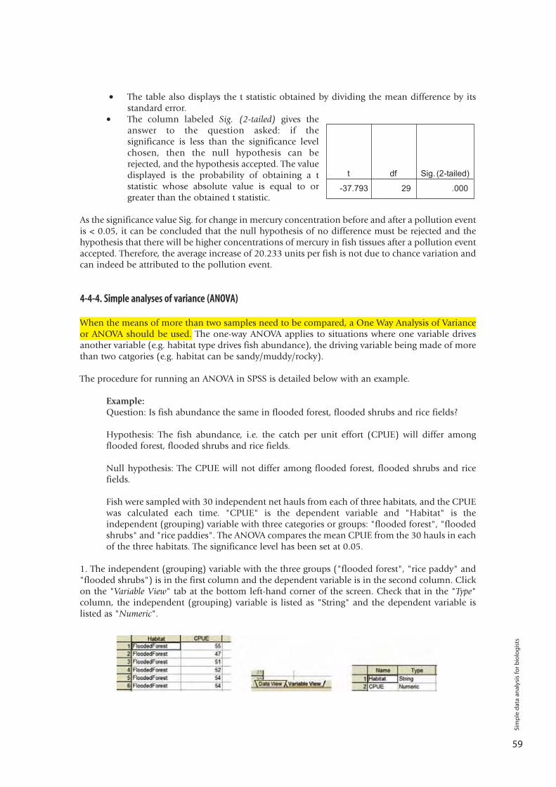
59

• The table also displays the t statistic obtained by dividing the mean difference by its standard error.

• The column labeled Sig. (2-tailed) gives the answer to the question asked: if thesignificance is less than the significance level chosen, then the null hypothesis can be rejected, and the hypothesis accepted. The value displayed is the probability of obtaining a tstatistic whose absolute value is equal to or greater than the obtained t statistic.

As the significance value Sig. for change in mercury concentration before and after a pollution eventis < 0.05, it can be concluded that the null hypothesis of no difference must be rejected and thehypothesis that there will be higher concentrations of mercury in fish tissues after a pollution eventaccepted. Therefore, the average increase of 20.233 units per fish is not due to chance variation andcan indeed be attributed to the pollution event.

4-4-4. Simple analyses of variance (ANOVA)

When the means of more than two samples need to be compared, a One Way Analysis of Varianceor ANOVA should be used. The one-way ANOVA applies to situations where one variable drivesanother variable (e.g. habitat type drives fish abundance), the driving variable being made of morethan two catgories (e.g. habitat can be sandy/muddy/rocky).

The procedure for running an ANOVA in SPSS is detailed below with an example.

Example:Question: Is fish abundance the same in flooded forest, flooded shrubs and rice fields?

Hypothesis: The fish abundance, i.e. the catch per unit effort (CPUE) will differ amongflooded forest, flooded shrubs and rice fields.

Null hypothesis: The CPUE will not differ among flooded forest, flooded shrubs and ricefields.

Fish were sampled with 30 independent net hauls from each of three habitats, and the CPUEwas calculated each time. "CPUE" is the dependent variable and "Habitat" is theindependent (grouping) variable with three categories or groups: "flooded forest", "floodedshrubs" and "rice paddies". The ANOVA compares the mean CPUE from the 30 hauls in eachof the three habitats. The significance level has been set at 0.05.

1. The independent (grouping) variable with the three groups ("flooded forest", "rice paddy" and"flooded shrubs") is in the first column and the dependent variable is in the second column. Clickon the "Variable View" tab at the bottom left-hand corner of the screen. Check that in the "Type"column, the independent (grouping) variable is listed as "String" and the dependent variable islisted as "Numeric".

Sim

ple

dat

a an

alys

is fo

r b

iolo

gis

ts

t df Sig. (2-tailed)

-37.793 29 .000

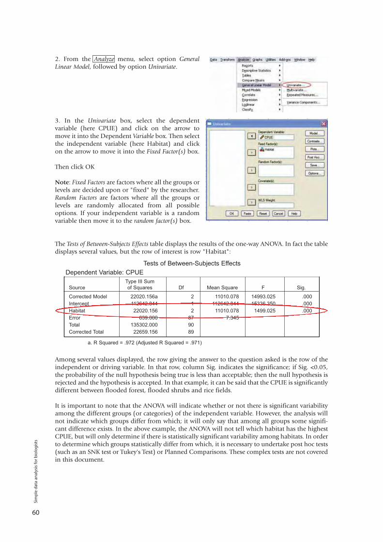
60

2. From the Analyze menu, select option GeneralLinear Model, followed by option Univariate.

3. In the Univariate box, select the dependentvariable (here CPUE) and click on the arrow tomove it into the Dependent Variable box. Then selectthe independent variable (here Habitat) and clickon the arrow to move it into the Fixed Factor(s) box.

Then click OK

Note: Fixed Factors are factors where all the groups orlevels are decided upon or "fixed" by the researcher.Random Factors are factors where all the groups orlevels are randomly allocated from all possibleoptions. If your independent variable is a randomvariable then move it to the random factor(s) box.

The Tests of Between-Subjects Effects table displays the results of the one-way ANOVA. In fact the tabledisplays several values, but the row of interest is row "Habitat":

Among several values displayed, the row giving the answer to the question asked is the row of theindependent or driving variable. In that row, column Sig. indicates the significance; if Sig. <0.05,the probability of the null hypothesis being true is less than acceptable; then the null hypothesis isrejected and the hypothesis is accepted. In that example, it can be said that the CPUE is significantlydifferent between flooded forest, flooded shrubs and rice fields.

It is important to note that the ANOVA will indicate whether or not there is significant variabilityamong the different groups (or categories) of the independent variable. However, the analysis willnot indicate which groups differ from which; it will only say that among all groups some signifi-cant difference exists. In the above example, the ANOVA will not tell which habitat has the highestCPUE, but will only determine if there is statistically significant variability among habitats. In orderto determine which groups statistically differ from which, it is necessary to undertake post hoc tests(such as an SNK test or Tukey's Test) or Planned Comparisons. These complex tests are not coveredin this document.

Type III SumSource of Squares Df Mean Square F Sig.

Corrected Model 22020.156a 2 11010.078 14993.025 .000Intercept 112642.844 1 112642.844 15336.350 .000Habitat 22020.156 2 11010.078 1499.025 .000Error 639.000 87 7.345Total 135302.000 90Corrected Total 22659.156 89

Tests of Between-Subjects EffectsDependent Variable: CPUE

a. R Squared = .972 (Adjusted R Squared = .971)

Sim

ple

dat

a an

alys

is fo

r b

iolo

gis

ts

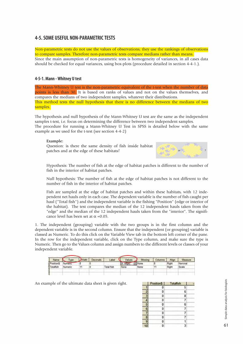
61

4-5. SOME USEFUL NON-PARAMETRIC TESTS

Non-parametric tests do not use the values of observations; they use the rankings of observationsto compare samples. Therefore non-parametric tests compare medians rather than means.Since the main assumption of non-parametric tests is homogeneity of variances, in all cases datashould be checked for equal variances, using box-plots (procedure detailed in section 4-4-1.).

4-5-1. Mann - Whitney U test

The Mann-Whitney U test is the non-parametric equivalent of the t-test when the number of datapoints is less than 30. It is based on ranks of values and not on the values themselves, andcompares the medians of two independent samples, whatever their distributions. This method tests the null hypothesis that there is no difference between the medians of twosamples.

The hypothesis and null hypothesis of the Mann-Whitney U test are the same as the independentsamples t-test, i.e. focus on determining the difference between two independent samples. The procedure for running a Mann-Whitney U Test in SPSS is detailed below with the sameexample as we used for the t-test (see section 4-4-2)

Example:Question: is there the same density of fish inside habitatpatches and at the edge of these habitats?

Hypothesis: The number of fish at the edge of habitat patches is different to the number offish in the interior of habitat patches.

Null hypothesis: The number of fish at the edge of habitat patches is not different to thenumber of fish in the interior of habitat patches.

Fish are sampled at the edge of habitat patches and within these habitats, with 12 inde-pendent net hauls only in each case. The dependent variable is the number of fish caught perhaul ("Total fish") and the independent variable is the fishing "Position" (edge or interior ofthe habitat). The test compares the median of the 12 independent hauls taken from the"edge" and the median of the 12 independent hauls taken from the "interior". The signifi-cance level has been set at α =0.05.

1. The independent (grouping) variable with the two groups is in the first column and thedependent variable is in the second column. Ensure that the independent (or grouping) variable isclassed as Numeric. To do this click on the Variable View tab in the bottom left corner of the pane.In the row for the independent variable, click on the Type column, and make sure the type isNumeric. Then go to the Values column and assign numbers to the different levels or classes of yourindependent variable.

An example of the ultimate data sheet is given right.

Sim

ple

dat

a an

alys

is fo

r b

iolo

gis

ts

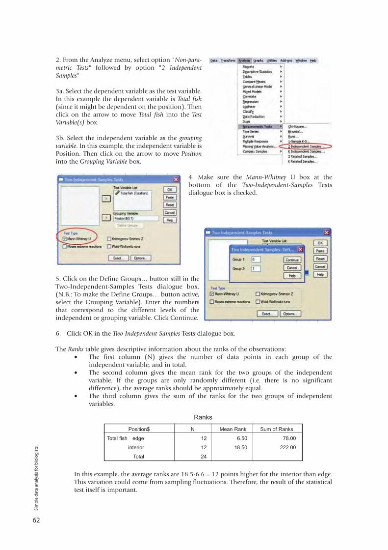
2. From the Analyze menu, select option "Non-para-metric Tests" followed by option "2 IndependentSamples"

3a. Select the dependent variable as the test variable.In this example the dependent variable is Total fish(since it might be dependent on the position). Thenclick on the arrow to move Total fish into the TestVariable(s) box.

3b. Select the independent variable as the groupingvariable. In this example, the independent variable isPosition. Then click on the arrow to move Positioninto the Grouping Variable box.

4. Make sure the Mann-Whitney U box at thebottom of the Two-Independent-Samples Testsdialogue box is checked.

5. Click on the Define Groups… button still in theTwo-Independent-Samples Tests dialogue box.(N.B.: To make the Define Groups… button active,select the Grouping Variable). Enter the numbersthat correspond to the different levels of theindependent or grouping variable. Click Continue.

6. Click OK in the Two-Independent-Samples Tests dialogue box.

The Ranks table gives descriptive information about the ranks of the observations: • The first column (N) gives the number of data points in each group of the

independent variable, and in total.• The second column gives the mean rank for the two groups of the independent

variable. If the groups are only randomly different (i.e. there is no significantdifference), the average ranks should be approximately equal.

• The third column gives the sum of the ranks for the two groups of independentvariables.

In this example, the average ranks are 18.5-6.6 = 12 points higher for the interior than edge.This variation could come from sampling fluctuations. Therefore, the result of the statisticaltest itself is important.

62

Position$ N Mean Rank Sum of Ranks

Total fish edge 12 6.50 78.00

interior 12 18.50 222.00

Total 24

Ranks

Sim

ple

dat

a an

alys

is fo

r b

iolo

gis

ts

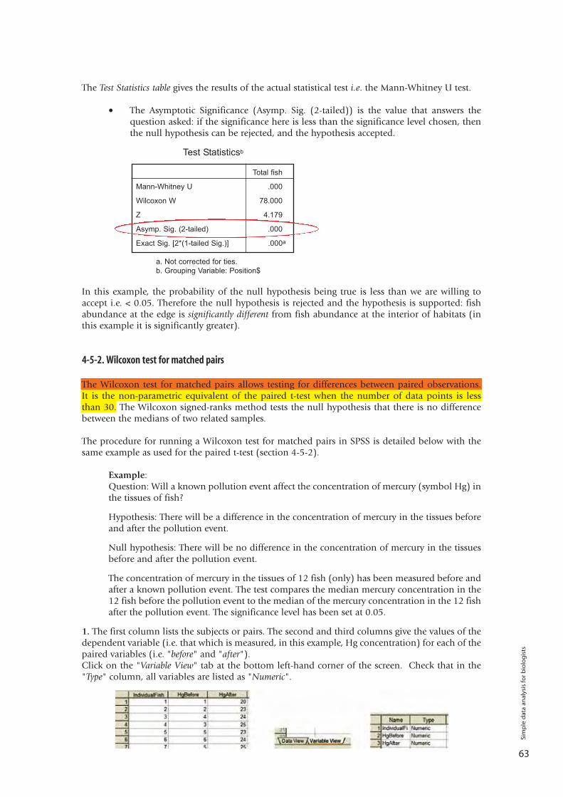
The Test Statistics table gives the results of the actual statistical test i.e. the Mann-Whitney U test.

• The Asymptotic Significance (Asymp. Sig. (2-tailed)) is the value that answers thequestion asked: if the significance here is less than the significance level chosen, then the null hypothesis can be rejected, and the hypothesis accepted.

In this example, the probability of the null hypothesis being true is less than we are willing toaccept i.e. < 0.05. Therefore the null hypothesis is rejected and the hypothesis is supported: fishabundance at the edge is significantly different from fish abundance at the interior of habitats (inthis example it is significantly greater).

4-5-2. Wilcoxon test for matched pairs

The Wilcoxon test for matched pairs allows testing for differences between paired observations.It is the non-parametric equivalent of the paired t-test when the number of data points is lessthan 30. The Wilcoxon signed-ranks method tests the null hypothesis that there is no differencebetween the medians of two related samples.

The procedure for running a Wilcoxon test for matched pairs in SPSS is detailed below with thesame example as used for the paired t-test (section 4-5-2).

Example:Question: Will a known pollution event affect the concentration of mercury (symbol Hg) inthe tissues of fish?

Hypothesis: There will be a difference in the concentration of mercury in the tissues beforeand after the pollution event.

Null hypothesis: There will be no difference in the concentration of mercury in the tissuesbefore and after the pollution event.

The concentration of mercury in the tissues of 12 fish (only) has been measured before andafter a known pollution event. The test compares the median mercury concentration in the12 fish before the pollution event to the median of the mercury concentration in the 12 fishafter the pollution event. The significance level has been set at 0.05.

1. The first column lists the subjects or pairs. The second and third columns give the values of thedependent variable (i.e. that which is measured, in this example, Hg concentration) for each of thepaired variables (i.e. "before" and "after").Click on the "Variable View" tab at the bottom left-hand corner of the screen. Check that in the"Type" column, all variables are listed as "Numeric".

63

Total fish

Mann-Whitney U .000

Wilcoxon W 78.000

Z 4.179

Asymp. Sig. (2-tailed) .000

Exact Sig. [2*(1-tailed Sig.)] .000a

Test Statisticsb

a. Not corrected for ties.b. Grouping Variable: Position$

Sim

ple

dat

a an

alys

is fo

r b

iolo

gis

ts

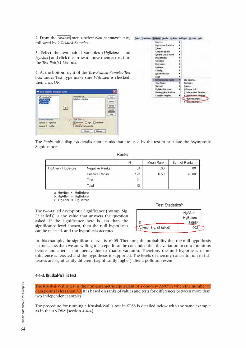
64

2. From the Analyze menu, select Non-parametric tests,followed by 2 Related Samples…

3. Select the two paired variables (HgBefore andHgAfter) and click the arrow to move them across intothe Test Pair(s) List box.

4. At the bottom right of the Two-Related-Samples-Testbox under Test Type make sure Wilcoxon is checked,then click OK.

The Ranks table displays details about ranks that are used by the test to calculate the AsymptoticSignificance:

The two-tailed Asymptotic Significance (Aysmp. Sig.(2 tailed)) is the value that answers the questionasked: if the significance here is less than thesignificance level chosen, then the null hypothesiscan be rejected, and the hypothesis accepted.

In this example, the significance level is <0.05. Therefore, the probability that the null hypothesisis true is less than we are willing to accept. It can be concluded that the variation in concentrationsbefore and after is not merely due to chance variation. Therefore, the null hypothesis of nodifference is rejected and the hypothesis it supported. The levels of mercury concentration in fishtissues are significantly different (significantly higher) after a pollution event.

4-5-3. Kruskal-Wallis test

The Kruskal-Wallis test is the non-parametric equivalent of a one-way ANOVA when the number ofdata points is less than 30. It is based on ranks of values and tests for differences between more thantwo independent samples.

The procedure for running a Kruskal-Wallis test in SPSS is detailed below with the same exampleas in the ANOVA (section 4-4-4).

Ranks

N Mean Rank Sum of Ranks

HgAfter - HgBefore Negative Ranks 0a .00 .00

Positive Ranks 12b 6.50 78.00

Ties 0c

Total 12

a. HgAfter < HgBeforeb. HgAfter > HgBeforeC. HgAfter = HgBefore

Test Statisticsb

HgAfter - HgBefore

Z -3.066a

Asymp. Sig. (2-tailed) .002

Sim

ple

dat

a an

alys

is fo

r b

iolo

gis

ts

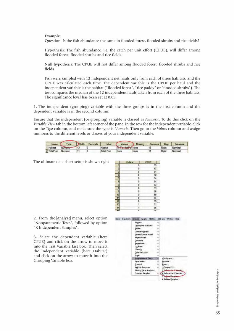
65

Example:Question: Is the fish abundance the same in flooded forest, flooded shrubs and rice fields?

Hypothesis: The fish abundance, i.e. the catch per unit effort (CPUE), will differ amongflooded forest, flooded shrubs and rice fields.

Null hypothesis: The CPUE will not differ among flooded forest, flooded shrubs and ricefields.

Fish were sampled with 12 independent net hauls only from each of three habitats, and theCPUE was calculated each time. The dependent variable is the CPUE per haul and theindependent variable is the habitat ("flooded forest", "rice paddy" or "flooded shrubs"). Thetest compares the median of the 12 independent hauls taken from each of the three habitats.The significance level has been set at 0.05.

1. The independent (grouping) variable with the three groups is in the first column and thedependent variable is in the second column.

Ensure that the independent (or grouping) variable is classed as Numeric. To do this click on theVariable View tab in the bottom left corner of the pane. In the row for the independent variable, clickon the Type column, and make sure the type is Numeric. Then go to the Values column and assignnumbers to the different levels or classes of your independent variable.

The ultimate data sheet setup is shown right

2. From the Analyze menu, select option"Nonparametric Tests", followed by option"K Independent Samples".

3. Select the dependent variable (hereCPUE) and click on the arrow to move itinto the Test Variable List box. Then selectthe independent variable (here Habitat)and click on the arrow to move it into theGrouping Variable box.

Sim

ple

dat

a an

alys

is fo

r b

iolo

gis

ts

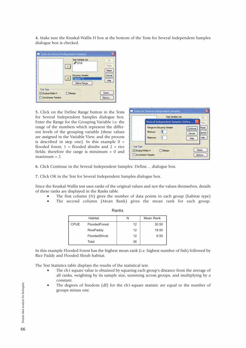
66

4. Make sure the Kruskal-Wallis H box at the bottom of the Tests for Several Independent Samplesdialogue box is checked.

5. Click on the Define Range button in the Testsfor Several Independent Samples dialogue box.Enter the Range for the Grouping Variable i.e. therange of the numbers which represent the differ-ent levels of the grouping variable (these valuesare assigned in the Variable View, and the processis described in step one). In this example 0 =flooded forest; 1 = flooded shrubs and 2 = ricefields; therefore the range is minimum = 0 andmaximum = 2.

6. Click Continue in the Several Independent Samples: Define… dialogue box.

7. Click OK in the Test for Several Independent Samples dialogue box.

Since the Kruskal-Wallis test uses ranks of the original values and not the values themselves, detailsof these ranks are displayed in the Ranks table.

• The first column (N) gives the number of data points in each group (habitat type)• The second column (Mean Rank) gives the mean rank for each group.

In this example Flooded Forest has the highest mean rank (i.e. highest number of fish) followed byRice Paddy and Flooded Shrub habitat.

The Test Statistics table displays the results of the statistical test.• The ch1-square value is obtained by squaring each group's distance from the average of

all ranks, weighting by its sample size, summing across groups, and multiplying by a constant.

• The degrees of freedom (df) for the ch1-square statistic are equal to the number of groups minus one.

Ranks

Habitat N Mean Rank

CPUE FloodedForest 12 30.50

RicePaddy 12 18.50

FloodedShrub 12 6.50

Total 36

Sim

ple

dat

a an

alys

is fo

r b

iolo

gis

ts

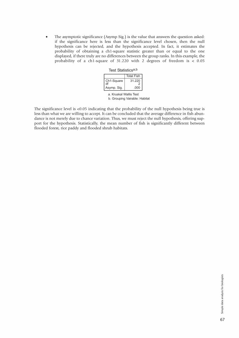
67

• The asymptotic significance (Asymp Sig.) is the value that answers the question asked: if the significance here is less than the significance level chosen, then the null hypothesis can be rejected, and the hypothesis accepted. In fact, it estimates theprobability of obtaining a ch1-square statistic greater than or equal to the onedisplayed, if there truly are no differences between the group ranks. In this example, the probability of a ch1-square of 31.220 with 2 degrees of freedom is < 0.05

The significance level is <0.05 indicating that the probability of the null hypothesis being true isless than what we are willing to accept. It can be concluded that the average difference in fish abun-dance is not merely due to chance variation. Thus, we must reject the null hypothesis, offering sup-port for the hypothesis. Statistically, the mean number of fish is significantly different betweenflooded forest, rice paddy and flooded shrub habitats.

Sim

ple

dat

a an

alys

is fo

r b

iolo

gis

ts

Total FishCh1-Square 31.220df 2Asymp. Sig. .000

Test Statisticsa,b

a. Kruskal Wallis Testb. Grouping Vairable: Habitat

Layout and print by Digital Graphic

WorldFish Center -Greater Mekong Region

P.O. Box 1135(Wat Phnom)

#35, Street 71, SangkatBeng Keng Kang 1,

Phnom Penh, CambodiaE-mail:

worldfish-cambodia@cgiar.org

Fisheries Administrationand IFReDI

#186, Norodom Blvd.,P.O. Box 582,

Phnom Penh, Cambodia.

SIMPLE DATA ANALYSISFOR BIOLOGISTS

Eric BARAN, Fiona WARRY

This book is a simple introduction to research methodsand analysis tools for biologists or environmentalscientists, with particular emphasis on fish biology indeveloping countries.

Financed by The WorldFish Center, the Asian Development Bank, AusAID and the European Union.