Simon Fraser Universitysummit.sfu.ca/system/files/iritems1/10018/etd5925.pdf · Abstract Wireless...
82
EQUALIZATION TECHNIQUES FOR BROADBAND WIRELESS NETWORKS by Homa Eghbali B.A.Sc., American University of Sharjah, Sharjah, U.A.E, 2009 Thesis submitted in partial fulfillment of the requirements for the degree of Masters of Science In the School of Engineering Science c Homa Eghbali 2010 SIMON FRASER UNIVERSITY Spring 2010 All rights reserved. However, in accordance with the Copyright Act of Canada, this work may be reproduced, without authorization, under the conditions for Fair Dealing. Therefore, limited reproduction of this work for the purposes of private study, research, criticism, review and news reporting is likely to be in accordance with the law, particularly if cited appropriately.
Transcript of Simon Fraser Universitysummit.sfu.ca/system/files/iritems1/10018/etd5925.pdf · Abstract Wireless...

EQUALIZATION TECHNIQUES FOR BROADBAND
WIRELESS NETWORKS
by
Homa Eghbali
B.A.Sc., American University of Sharjah, Sharjah, U.A.E, 2009
Thesis submitted in partial fulfillment
of the requirements for the degree of
Masters of Science
In the School
of
Engineering Science
c© Homa Eghbali 2010
SIMON FRASER UNIVERSITY
Spring 2010
All rights reserved. However, in accordance with the Copyright Act of Canada,
this work may be reproduced, without authorization, under the conditions for Fair
Dealing. Therefore, limited reproduction of this work for the purposes of private
study, research, criticism, review and news reporting is likely to be in
accordance with the law, particularly if cited appropriately.


Last revision: Spring 09
Declaration of Partial Copyright Licence The author, whose copyright is declared on the title page of this work, has granted to Simon Fraser University the right to lend this thesis, project or extended essay to users of the Simon Fraser University Library, and to make partial or single copies only for such users or in response to a request from the library of any other university, or other educational institution, on its own behalf or for one of its users.
The author has further granted permission to Simon Fraser University to keep or make a digital copy for use in its circulating collection (currently available to the public at the “Institutional Repository” link of the SFU Library website <www.lib.sfu.ca> at: <http://ir.lib.sfu.ca/handle/1892/112>) and, without changing the content, to translate the thesis/project or extended essays, if technically possible, to any medium or format for the purpose of preservation of the digital work.
The author has further agreed that permission for multiple copying of this work for scholarly purposes may be granted by either the author or the Dean of Graduate Studies.
It is understood that copying or publication of this work for financial gain shall not be allowed without the author’s written permission.
Permission for public performance, or limited permission for private scholarly use, of any multimedia materials forming part of this work, may have been granted by the author. This information may be found on the separately catalogued multimedia material and in the signed Partial Copyright Licence.
While licensing SFU to permit the above uses, the author retains copyright in the thesis, project or extended essays, including the right to change the work for subsequent purposes, including editing and publishing the work in whole or in part, and licensing other parties, as the author may desire.
The original Partial Copyright Licence attesting to these terms, and signed by this author, may be found in the original bound copy of this work, retained in the Simon Fraser University Archive.
Simon Fraser University Library Burnaby, BC, Canada
Abstract
Wireless sensor networks (WSNs) are characterized by low-power devices equipped with
communication capabilities. Due to the lack of a set infrastructure, WSNs exhibit char-
acteristics fundamentally different from traditional networks. The existing literature in
conventional wireless networks, therefore, cannot be applied to WSN design.
The recently introduced Cooperative diversity techniques exploit the broadcast nature
of wireless transmission, creating a virtual antenna array through cooperating nodes. This
form of diversity is therefore well suited for WSNs. The research in this field is however,
still in it’s infancy. Particularly, most of the current literature in this area assumes an
idealized transmission environment with an underlying frequency-flat fading channel model
and perfect channel state information, which are far away from being realistic if wideband
sensor applications or mobile sensor networks are considered.
Motivated by these practical concerns, this thesis addresses the analysis and design of
efficient equalization techniques for non-cooperative and cooperative wireless networks.
iii

Dedication
To My Dearest Parents and My Lovely Brother
iv

Acknowledgement
I wish to thank my loving parents. Without their endless love, knowledge, wisdom, and
guidance, I would not have the goals I have to strive and reach my dreams. I am heartily
thankful to my senior supervisor, Professor Sami Muhaidat, whose encouragement, guidance
and support from the initial to the final level enabled me to develop an understanding of
the subject. I would like to thank Professor Naofal Al-Dhahir from university of Texas at
Dallas and Professor Murat Uysal from university of Waterloo for their helpful cooperation.
I would also like to thank Professor Rodney G. Vaughan for serving on my supervisory
committee and Professor Paul K. M. Ho for serving as the internal examiner of my thesis.
It is also my honor to thank the defense chair, Professor Jie Liang, for his time and efforts.
Lastly, I offer my regards and blessings to all of those who supported me in any respect
during the completion of the project. Special thanks go to the current and past members
of our lab, Jinyun Ren, Maryam Dehghan, Sayed Alireza Banani, and Saad Mahboob to
name but a few, for their help and lively discussions on research, and beyond.
Homa
v
Publications
1) H. Eghbali, S. Muhaidat, and N. Al-Dhahir, “A Novel Receiver Design for Single-
Carrier Frequency Domain Equalization in Broadband Wireless Networks with Amplify-and-
Forward Relaying,” Accepted to IEEE Transactions on Wireless Communications, January
2010
2) H. Eghbali, S. Muhaidat, and N. Al-Dhahir, “A New Reduced Complexity Detection
Scheme for Zero-Padded OFDM Transmissions,” submitted to IEEE Transactions on Sig-
nal Processing as a Correspondence, February 2010
3) H. Eghbali, S. Muhaidat, and N. Al-Dhahir, “A Low Complexity two Stage MMSE-Based
Receiver for Single-Carrier Frequency-Domain Equalization Transmissions over Frequency-
Selective Channels,” IEEE GLOBECOM’09, Honolulu, Hawaii, USA, November 2009.
4) H. Eghbali, and M. El-Tarhuni, “Multipath Detection for TH-PPM UWB Systems,”
ISSPIT2009, Ajman, U.A.E , December 2009.
5) H. Eghbali, S. Muhaidat, and N. Al-Dhahir, “A Novel Reduced Complexity MMSE-based
Receiver for OFDM Broadband Wireless Networks,” IEEE WCNC 2010, Sydney, Australia,
April 2010.
6) H. Eghbali, S. Muhaidat, and N. Al-Dhahir, “A Novel Reduced Complexity Detection
Scheme for Distributed Single-Carrier Frequency Domain Equalization,” to be submitted
to IEEE VTC 2010.
7) H. Eghbali, S. Muhaidat, and N. Al-Dhahir, “Performance Analysis of Distributed Space-
Time Block Codes Using Frequency Domain Equalization Techniques Over Nakagami-n
fading Channels,” to be submitted to IEEE GLOBECOM’10.
8) H. Eghbali, S. Muhaidat, and N. Al-Dhahir, “A New Receiver Design for Single-Carrier
Frequency-Domain Equalization in Broadband Cooperative Networks ,” to be submitted to
IEEE GLOBECOM’10.
vi
Contents
Approval ii
Abstract iii
Dedication iv
Acknowledgement v
Publications vi
Contents vii
List of Tables x
List of Figures xi
1 Introduction 1
1.1 Thesis Motivation . . . . . . . . . . . . . . . . . . . . . . . . . . . . . . . . 1
1.2 Outline and Main Contributions . . . . . . . . . . . . . . . . . . . . . . . . 2
1.3 Notations and Acronyms . . . . . . . . . . . . . . . . . . . . . . . . . . . . . 5
2 Background 8
2.1 Introduction . . . . . . . . . . . . . . . . . . . . . . . . . . . . . . . . . . . . 8
2.2 Diversity Techniques for Fading Channels . . . . . . . . . . . . . . . . . . . 9
2.2.1 Time Diversity . . . . . . . . . . . . . . . . . . . . . . . . . . . . . . 10
2.2.2 Frequency Diversity . . . . . . . . . . . . . . . . . . . . . . . . . . . 10
2.2.3 Space Diversity . . . . . . . . . . . . . . . . . . . . . . . . . . . . . . 10
vii

2.2.4 Diversity Combining Techniques . . . . . . . . . . . . . . . . . . . . 11
2.3 Transmit Diversity . . . . . . . . . . . . . . . . . . . . . . . . . . . . . . . . 11
2.4 Space-Time Coding . . . . . . . . . . . . . . . . . . . . . . . . . . . . . . . . 13
2.5 Cooperative Diversity . . . . . . . . . . . . . . . . . . . . . . . . . . . . . . 16
2.6 Orthogonal frequency division multiplexing . . . . . . . . . . . . . . . . . . 19
2.7 Single-carrier frequency domain equalization . . . . . . . . . . . . . . . . . . 20
2.8 Summary . . . . . . . . . . . . . . . . . . . . . . . . . . . . . . . . . . . . . 21
3 A New Detection Scheme for Zero-Padded OFDM 22
3.1 Introduction . . . . . . . . . . . . . . . . . . . . . . . . . . . . . . . . . . . . 22
3.2 Overview . . . . . . . . . . . . . . . . . . . . . . . . . . . . . . . . . . . . . 22
3.3 System Model . . . . . . . . . . . . . . . . . . . . . . . . . . . . . . . . . . . 24
3.4 Reduced complexity MMSE-based receiver . . . . . . . . . . . . . . . . . . . 25
3.5 Computational Complexity Analysis . . . . . . . . . . . . . . . . . . . . . . 27
3.6 Numerical Results . . . . . . . . . . . . . . . . . . . . . . . . . . . . . . . . 28
3.7 Summary . . . . . . . . . . . . . . . . . . . . . . . . . . . . . . . . . . . . . 29
4 MMSE-Based Receiver Design for Single-Carrier Frequency Domain Equal-
ization 34
4.1 Introduction . . . . . . . . . . . . . . . . . . . . . . . . . . . . . . . . . . . . 34
4.2 System Model . . . . . . . . . . . . . . . . . . . . . . . . . . . . . . . . . . . 35
4.3 MMSE-based receiver for D-SC-STBC . . . . . . . . . . . . . . . . . . . . . 36
4.4 Diversity Gain Analysis . . . . . . . . . . . . . . . . . . . . . . . . . . . . . 40
4.5 Computational Complexity Analysis . . . . . . . . . . . . . . . . . . . . . . 45
4.6 Numerical Results . . . . . . . . . . . . . . . . . . . . . . . . . . . . . . . . 46
4.7 Summary . . . . . . . . . . . . . . . . . . . . . . . . . . . . . . . . . . . . . 49
5 Distributed Single-Carrier Frequency Domain Equalization in Multi-Relay
Networks. 50
5.1 introduction . . . . . . . . . . . . . . . . . . . . . . . . . . . . . . . . . . . . 50
5.2 overview . . . . . . . . . . . . . . . . . . . . . . . . . . . . . . . . . . . . . . 50
5.3 Transmission Model . . . . . . . . . . . . . . . . . . . . . . . . . . . . . . . 51
5.4 Diversity Gain Analysis . . . . . . . . . . . . . . . . . . . . . . . . . . . . . 55
5.5 Numerical Results . . . . . . . . . . . . . . . . . . . . . . . . . . . . . . . . 60
viii
5.6 Summary . . . . . . . . . . . . . . . . . . . . . . . . . . . . . . . . . . . . . 63
6 Conclusion 64
6.1 Conclusions . . . . . . . . . . . . . . . . . . . . . . . . . . . . . . . . . . . . 64
6.2 Future works . . . . . . . . . . . . . . . . . . . . . . . . . . . . . . . . . . . 65
Bibliography 66
ix

List of Tables
1.1 List of notations. . . . . . . . . . . . . . . . . . . . . . . . . . . . . . . . . . 5
1.2 List of acronyms. . . . . . . . . . . . . . . . . . . . . . . . . . . . . . . . . . 7
2.1 Cooperation protocols for single-relay networks. . . . . . . . . . . . . . . . . 19
3.1 Comparison of overall computational complexity in the HL2. . . . . . . . . 28
4.1 Comparison of overall computational complexity. . . . . . . . . . . . . . . . 46
x

List of Figures
2.1 Block diagram of a space-time coded system. . . . . . . . . . . . . . . . . . 13
2.2 Relay assisted transmission. . . . . . . . . . . . . . . . . . . . . . . . . . . . 17
2.3 OFDM and SC-FDE– signal processing similarities and differences. . . . . . 21
3.1 Proposed low-complexity MMSE-ZP-OFDM receiver block diagram. . . . . 30
3.2 Computational complexity of the proposed receiver compared to ZP-OFDM-
MMSE. . . . . . . . . . . . . . . . . . . . . . . . . . . . . . . . . . . . . . . 31
3.3 BER performance of ZP-OFDM-MMSE, single stage receiver and proposed
receiver, uniform power-delay profile (L =3). . . . . . . . . . . . . . . . . . 31
3.4 BER performance of ZP-OFDM-MMSE, single stage receiver and proposed
receiver, uniform power-delay profile (L =4). . . . . . . . . . . . . . . . . . 32
3.5 BER performance of ZP-OFDM-MMSE, single stage receiver and proposed
receiver, exponential power-delay profile (L =6). . . . . . . . . . . . . . . . 32
3.6 BER performance of ZP-OFDM-MMSE, single stage receiver and proposed
receiver, exponential power-delay profile (L =7). . . . . . . . . . . . . . . . 33
4.1 Percentage increase in the computational complexity of the proposed receiver
compared to MMSE-D-SC-STBC. . . . . . . . . . . . . . . . . . . . . . . . 45
4.2 SER performance of MMSE-D-STBC-SC and proposed receiver. . . . . . . 46
4.3 SER performance of MMSE-D-STBC-SC and proposed receiver. . . . . . . 47
4.4 SER performance of MMSE-D-STBC-SC and proposed receiver. . . . . . . 47
5.1 SER performance of the DSTBC SC-FDE system with two relays. . . . . . 60
5.2 SER performance of the DSTBC SC-FDE system with three relays. . . . . 61
5.3 SER performance of the DSTBC SC-FDE system for different K-factor values. 62
xi

Chapter 1
Introduction
1.1 Thesis Motivation
Recent advances in miniaturization and low-cost, low-power electronics have led to active
research in large-scale networks of small, wireless, low-power sensors and actuators. Per-
vasive sensing that is freed from the burden of infrastructure will revolutionize the way we
observe the world around us. Sensor networks already automatically warn us of invisible
hazards, i.e. the contaminants in the air we breath or the water we drink, and far-away
earthquakes soon to arrive. WSNs can open the eyes of a new generation of scientist to
phenomena never before observable, paving the way to new eras of understanding in the
natural sciences. These networks are characterized by small, low-power devices equipped
with sensing and communication capabilities. With numerous applications and impact on
several industries, WSNs are envisioned to be a key technology area for enormous growth
in the near future. WSNs exhibit characteristics fundamentally different from traditional
networks, due to the lack of a set infrastructure. Therefore, it’s not possible to apply the
existing rich literature in conventional wireless networks to WSN designs.
Cooperative diversity is a form of diversity well studied for WSNs, exploiting the broad-
cast nature of wireless transmissions by creating a virtual antenna array through cooperative
nodes. Although cooperative diversity has recently gained much attention, research in this
field is still in its infancy. The pioneering works in this area address mainly information-
theoretic aspects, deriving fundamental performance bounds. However, practical implemen-
tation of cooperative diversity requires an in-depth investigation of several physical layer
1
CHAPTER 1. INTRODUCTION 2
issues such as channel estimation, equalization, and synchronization integrating the under-
lying cooperation protocols and relaying modes. Moreover, most of the current literature in
the area of cooperative diversity assume an idealized transmission environment with an un-
derlying frequency-flat fading channel model and perfect channel state information, which
can be justified for fixed infrastructure narrowband WSNs, but are far away from being
realistic for wideband sensor applications or mobile sensor networks.
Motivated by the practical concerns aforementioned, the main purpose of this thesis is
to investigate and develop low-power consuming and efficient equalization techniques for
non-distributed and distributed wireless networks.
1.2 Outline and Main Contributions
In chapter 2, we provide a brief review of important background materials related to the
thesis. We first review different diversity techniques for fading channels including time
diversity, frequency diversity, and space diversity, followed by an introduction to different
diversity combining techniques. We then introduce the important concepts that will be
used extensively throughout the thesis, including transmit diversity, space-time coding,
cooperative diversity, multi-carrier modulation schemes, single carrier frequency-domain
equalization (SC-FDE), orthogonal frequency division multiplexing (OFDM), and space-
time block coded (STBC) SC-FDE.
In chapter 3, we study a new detection scheme for zero-padding (ZP)-OFDM. Recently,
ZP-OFDM has been proposed as an alternative solution to coded-OFDM, which often incurs
high decoding complexity. Various ZP-OFDM receivers have been proposed in the literature,
trading off performance with complexity. To trade-off Bit Error Rate (BER) performance
for extra savings in complexity, two low complexity equalizers for ZP-OFDM are derived in
[1]. However, the BER performance of the two sub-optimal receivers proposed in [1] is not
as good as minimum mean square error (MMSE)-ZP-OFDM. We propose a novel reduced
complexity receiver design for ZP-OFDM transmissions, that not only outperforms MMSE-
ZP-OFDM, but also uses low-complexity computational methods that bring a significant
power saving to the proposed receiver. This makes it a strong candidate for WSNs which are
characterized by small and low-power devices. We show that linear processing collects both
multipath and spatial diversity gains, leading to significant improvement in performance,
while maintaining low complexity. The material of this chapter has appeared in [2].
CHAPTER 1. INTRODUCTION 3
In chapter 4, we introduce a novel MMSE-based receiver design for SC-FDE. Although
most of the current literature on SC-FDE is limited to point-to-point systems, there have
been recent results reported on FDE in the context of cooperative scenarios [3, 4]. dis-
tributed (D)-STBC SC-FDE has been discussed in [3], assuming the maximum likelihood
sequence detection (MLSD) equalization. Although significant diversity gains were demon-
strated, the complexity of MLSD equalizers increases with the channel memory, signal con-
stellation size, and the number of transmit/receive antennas. This, in turn, places significant
additional computational and power consumption loads on the receiver side. Therefore, low-
complexity equalization schemes without sacrificing performance are particularly desirable,
especially for cases where the receiver implementation is supposed to be simple and required
to operate on a limited battery power.
Building upon the work of [5], we propose a novel reduced-complexity MMSE-based re-
ceiver design for D-STBC SC-FDE transmissions. Specifically, we are considering amplify-
and-forward (AF) relay networks for cooperative scenarios in which either of source to relay
(S → R) or relay to destination (R → D) links are frequency selective Rician fading. We
justify this assumption, by presuming that the line-of-sight (LOS) path exists for either of
(S → R) or R → D) links. We show that, by incorporating linear processing techniques,
our MMSE-based receiver is able to collect full antenna and multipath diversity gains, lead-
ing to significant improvement in performance at nearly no additional complexity. Detailed
diversity order analysis and complexity analysis are presented to corroborate the proposed
system’s outperformance compared to the conventional cooperative MMSE-SC-FDE re-
ceiver. Specifically, under the assumption of perfect power control and high signal-to-noise
ratio (SNR) for the underlying links and assuming either of S → R or R → D links to be
frequency selective Rician fading, our performance analysis demonstrates that the proposed
receiver is able to achieve a maximum diversity order of min(LSR, LRD) + LSD + 2, where
LSR, LRD, and LSD are the channel memory lengths for S → R, R → D, and S → D
links, respectively. Complexity analysis and simulation results demonstrate that within
the bounds of the aforementioned system modeling and assumptions, our proposed receiver
outperforms the conventional cooperative MMSE-SC-FDE receiver by performing close to
matched filter bound (MFB).
In chapter 5, we investigate the performance of D-STBC SC-FDE systems with AF
relaying over frequency-selective Rician fading channels in multi-relay networks. Our per-
formance analysis demonstrates that SC-FDE for DSTBC is able to achieve a maximum

CHAPTER 1. INTRODUCTION 4
diversity order ofR∑
i=1min(LSRi , LRiD) + R, where R is the number of participating relays,
LSRi and LRiD are the channel memory lengths for source to ith relay (S → Ri) link and
ith relay to destination (Ri → D) link , respectively. Simulation results are provided to
corroborate the theoretical analysis.
Finally, we summarize the work in this thesis and present the conclusions in Chapter 6.

CHAPTER 1. INTRODUCTION 5
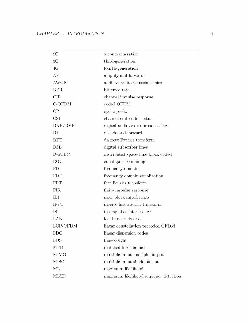
1.3 Notations and Acronyms
In this section we define the notations and acronyms used throughout this thesis.
a A boldface lowercase letter denotes a vector.
A A boldface uppercase letter denotes a matrix.−(.) Conjugate operation.
(.)T Transpose operation.
(.)H Hermitian transpose operation.
(.)−1 Inverse operation.
[.]k,l (k, l)th entry of a matrix.
[.]k kth entry of a vector.
IN identity matrix of size N .
0M×M all-zero matrix of size M ×M .
PN N ×N permutation matrix.
[PqNa]s a ((N − s + q) mod N), for a = [ a0 · · · aN−1]T .
Q N ×N FFT matrix with Q(l, k) = 1/√
N exp(−j2πlk/N).
Table 1.1: List of notations.
CHAPTER 1. INTRODUCTION 6
2G second-generation
3G third-generation
4G fourth-generation
AF amplify-and-forward
AWGN additive white Gaussian noise
BER bit error rate
CIR channel impulse response
C-OFDM coded OFDM
CP cyclic prefix
CSI channel state information
DAB/DVB digital audio/video broadcasting
DF decode-and-forward
DFT discrete Fourier transform
DSL digital subscriber lines
D-STBC distributed space-time block coded
EGC equal gain combining
FD frequency domain
FDE frequency domain equalization
FFT fast Fourier transform
FIR finite impulse response
IBI inter-block interference
IFFT inverse fast Fourier transform
ISI intersymbol interference
LAN local area networks
LCP-OFDM linear constellation precoded OFDM
LDC linear dispersion codes
LOS line-of-sight
MFB matched filter bound
MIMO multiple-input-multiple-output
MISO multiple-input-single-output
ML maximum likelihood
MLSD maximum likelihood sequence detection
CHAPTER 1. INTRODUCTION 7
MMSE minimum mean square error
MRC maximal ratio combining
NAF non-orthogonal amplify-and-forward
OFDM orthogonal frequency division multiplexing
OFDMA orthogonal frequency-division multiple access
pdf probability density function
PAR peak-to-average ratio
PEP pairwise error probability
PSK phase-shift keying
QAM quadrature amplitude modulation
SC selection combining
SC single carrier
SER symbol error rate
SIMO single-input-multiple-output
SNR signal-to-noise ratio
SO-STTC super-orthogonal space-time trellis coding
SR selection relaying
STBC space-time block codes
STTCs space-time trellis codes
TCM trellis-coded modulation
TD time domain
TDMA time-division multiple access
WPANs wireless personal area network
WSN wireless sensor networks
ZP zero padding
Table 1.2: List of acronyms.

Chapter 2
Background
2.1 Introduction
A glimpse of recent technological history reveals out that mobile communication systems
create a new generation roughly every 10 years. First-generation analogue systems were
introduced in the early 1980’s, then second-generation (2G) digital systems came in the
early 1990’s. Later, third-generation (3G) systems gradually unfolded all over the world
while intensive conceptual and research work toward the definition of a future system had
been already started.
2G systems, such as GSM and IS-95, were essentially designed for voice and low data
rate applications. In an effort to address customer demands for high-speed data communi-
cation, telecommunication companies have been launching 3G systems where the business
focus has shifted from voice services to multimedia communication applications over the
Internet. Despite the increasing penetration rate of 3G systems in the wireless market,
3G networks are challenged primarily in meeting the requirements imposed by the ever-
increasing demands of high-throughput multimedia and internet applications. Additionally,
3G systems consist primarily of wide area networks and thus fall short of supporting het-
erogeneous networks, including wireless local area networks (LANs) and wireless personal
area networks (WPANs).
Several wireless technologies co-exist in the current market customized for different
service types, data rates, and users. The next generation systems also known as the fourth
generation (4G) systems are envisioned to accommodate and integrate all existing and
future technologies in a single standard. The key feature of the 4G systems would be ”high
8
CHAPTER 2. BACKGROUND 9
usability” [6]; that is the user would be able to use the system at anytime, anywhere, and
with any technology. Users carrying an integrated wireless terminal would have access to a
variety of multimedia applications in a reliable environment at lower cost. To meet these
demands, next generation wireless communication systems must support high capacity and
variable bit rate information (adaptive) transmission with high bandwidth efficiency to
conserve limited spectrum resources.
2.2 Diversity Techniques for Fading Channels
The characteristics of the wireless channel impose fundamental limitations on the perfor-
mance of wireless communication systems. The wireless channel can be investigated by
decomposing it into two parts, i.e., large-scale (long-term) impairments including path loss,
shadowing and small-scale (short-term) impairment which is commonly referred as fading.
The former component is used to predict the average signal power at the receiver and the
transmission coverage area. The latter is due to the multipath propagation which causes
random fluctuations in the received signal level and affects the instantaneous SNR.
For a typical mobile wireless channel in urban areas where there is no LOS propagation
and the number of scatters is large, the application of central limit theory indicates that
the complex fading channel coefficient has two quadrature components which are zero-
mean Gaussian random processes. As a result, the amplitude of the fading envelope follows
a Rayleigh distribution. In terms of error rate performance, Rayleigh fading converts the
exponential dependency of the bit-error probability on the SNR for the additive white
Gaussian noise (AWGN) channel into an approximately inverse linear one, resulting in a
large SNR penalty.
A common approach to mitigate the degrading effects of fading is the use of diversity
techniques. Diversity improves transmission performance by making use of more than one
independently faded versions of the transmitted signal. If several replicas of the signals are
transmitted over multiple channels that exhibit independent fading with comparable average
strengths, the probability that all the independently faded signal components experience
deep fading simultaneously is significantly reduced.
There are various approaches to extract diversity from the wireless channel. The most
common methods are briefly summarized as follows [7, 8, 9]:
CHAPTER 2. BACKGROUND 10
2.2.1 Time Diversity
In this form of diversity, the same signal is transmitted in different time slots separated by
an interval longer than the coherence time of the channel. Channel coding in conjunction
with interleaving is an efficient technique to provide time diversity. In fast fading envi-
ronments where the mobility is high, time diversity becomes very efficient. However, for
slow-fading channel (e.g., low mobility environments, fixed-wireless applications), it offers
little protection unless significant interleaving delays can be tolerated.
2.2.2 Frequency Diversity
In this form of diversity, the same signal is sent over different frequency carriers, whose
separation must be larger than the coherence bandwidth of the channel to ensure indepen-
dence among diversity channels. Since multiple frequencies are needed, this is generally not
a bandwidth-efficient solution. A natural way of frequency diversity, which is sometimes
referred to as path diversity, arises for frequency-selective channels. When the multipath
delay spread is a significant fraction of the symbol period, the received signal can be in-
terpreted as a linear combination of the transmitted signal weighted by independent fading
coefficients. Therefore, path diversity is obtained by resolving the multipath components at
different delays using a RAKE correlator [7], which is the optimum receiver in the MMSE
sense designed for this type of channels.
2.2.3 Space Diversity
In this form of diversity, which is also sometimes called as antenna diversity, the receiver
and/or transmitter uses multiple antennas. This technique is especially attractive since
it does not require extra bandwidth. To extract full diversity advantages, the spacing
between antenna elements should be wide enough with respect to the carrier wavelength.
The required antenna separation depends on the local scattering environment as well as on
the carrier frequency. For a mobile station which is near the ground with many scatters
around, the channel decorrelates over shorter distances, and typical antenna separation of
half to one carrier wavelength is sufficient. For base stations on high towers, a larger antenna
separation of several to tens of wavelengths may be required.
CHAPTER 2. BACKGROUND 11
2.2.4 Diversity Combining Techniques
There exist different combining techniques, each of which can be used in conjunction with
any of the aforementioned diversity forms. The most common diversity combining tech-
niques are selection, equal gain and maximal ratio combining [7]. Selection combining (SC)
is conceptually the simplest; it consists of selecting at each time, among the available di-
versity branches (channels), the one with the largest value of SNR. Since it requires only
a measure of the powers received from each branch and a switch to choose among the
branches, it is relatively easy to implement. However, the fact that it disregards the in-
formation obtained from all branches except the selected one indicates its non-optimality.
In equal gain combining (EGC), the signals at the output of diversity branches are com-
bined linearly and the phase of the linear combination are selected to maximize the SNR
disregarding the amplitude differences. Since each branch is combined linearly, compared
to SC, EGC performs better. In maximal-ratio-combining (MRC), the signals at the output
of diversity branches are again combined linearly and the coefficients of the linear combina-
tion are selected to maximize the SNR regarding both the phase and the amplitude. The
MRC outperforms the other two, since it makes use of the both fading amplitude and phase
information. However, the difference between EGC and MRC is not considerably large in
terms of power efficiency; therefore, EGC can be preferred where implementation costs are
crucial. It should be emphasized that the effectiveness of any diversity scheme rests on the
availability of independently faded versions of the transmitted signal so that the probability
of two or more versions of the signal undergoing a deep fade is minimum. The reader can
refer to [7, 8, 9] and references therein for a broad overview of diversity combining systems.
2.3 Transmit Diversity
Space diversity, in the form of multiple antenna deployment at the receive side, has been
successfully used in uplink transmission (i.e., from mobile station to base station) of the
cellular communication systems [10]. However, the use of multiple receive antennas at the
mobile handset in the downlink transmission (i.e., from base station to mobile station) is
more difficult to implement because of size limitations and the expense of multiple down-
conversion of RF paths [11]. This motivates the use of multiple transmit antennas at the
base station in the downlink. Since a base station often serves many mobile stations, it
is also more economical to add hardware and additional signal processing to base stations
CHAPTER 2. BACKGROUND 12
rather than the mobile handsets. Despite its obvious advantages, transmit diversity has
traditionally been viewed as more difficult to exploit, in part because the transmitter is
assumed to know less about the channel than the receiver and in part because of the chal-
lenging signaling design problem. Within the last decade, transmit diversity has attracted
a great attention and practical solutions to realize transmit diversity advantages have been
proposed [9].
The transmit diversity techniques can be classified into two broad categories based on the
need for channel state information at the transmit side: Close loop schemes and open loop
schemes. The first category uses feedback, either explicitly or implicitly, from the receiver to
the transmitter to configure the transmitter. Close loop transmit diversity has more power
efficiency compared to open loop transmit diversity. However, it increases the overhead
of transmission and therefore is not bandwidth-efficient. Moreover, in practice, vehicle
movements or interference causes a mismatch between the state of the channel perceived by
the transmitter and that perceived by the receiver, making the feedback unreliable in some
situations.
In open loop transmit diversity schemes, feedback is not required. They use linear
processing at the transmitter to spread the information across multiple antennas. At the
receive side, information is recovered by either linear processing or maximum-likelihood de-
coding techniques. The first of such schemes was proposed by Wittneben [12, 13] where the
operating frequency-flat fading channel is converted intentionally into a frequency-selective
channel to exploit artificial path diversity by means of a maximum-likelihood decoder. It
was later shown in [14] that delay diversity schemes are optimal in providing diversity in
the sense that the diversity advantage experienced by an optimal receiver is equal to the
number of transmit antennas.
The linear filtering used to create delay diversity at the transmitter can be viewed as a
channel code which takes binary or integer input and creates real valued output. Therefore,
from a coding perspective, delay diversity schemes correspond to repetition codes and lead
to the natural question as to whether more sophisticated codes might be designed. The
challenge of designing channel codes for multiple-antenna systems has led to the introduction
of so-called space-time trellis codes by Tarokh, Seshadri and Calderbank [15].
CHAPTER 2. BACKGROUND 13
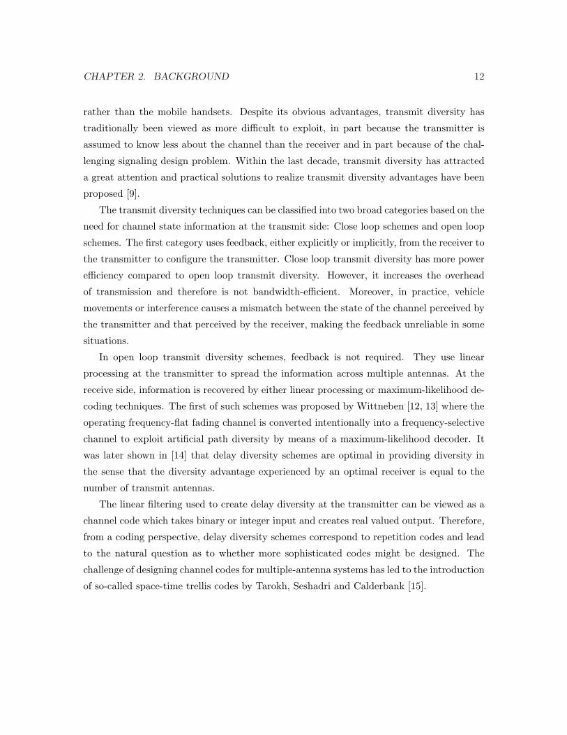
Figure 2.1: Block diagram of a space-time coded system.
2.4 Space-Time Coding
Space-time trellis codes (STTCs) combine the channel code design with symbol mapping
onto multiple transmit antennas. The data symbols are cleverly coded across space and time
to extract diversity advantages [15]. Figure 2.1 illustrates a space-time coded system. Let
space-time code be represented as a W ×MS matrix, where MS is the number of transmit
antennas and W is the codeword length. Each entry of X represents the modulation symbol
transmitted from the mthS (mS = 1, 2, ...MS) antenna during the wth (w = 1, 2, ...W ) symbol
period.
X =
x11 x1
2 ... x1MS
x21 ... ... x2
MS
: ... ... :
xW1 xW
2 ... xWMS
(2.1)
The signal at each receive antenna is a superposition of the MS transmitted signals
corrupted by fading. The received signal at the nth antenna within the wth symbol period
is given by
rwn =
MS∑
mS=1
hnmS
xwmS
+ nwn (2.2)
where hnmS
denotes the frequency flat fading coefficient from the mSth transmit antenna to
the nth receive antenna, that is considered to be quasi static constant over the codeword’s
length W . It is modeled as a complex Gaussian random variable with variance 0.5 per
dimension leading to the well-known Rayleigh fading channel model. In (2.2), nwn models
the additive noise term and is zero-mean complex Gaussian random variable with variance
N0/2 per dimension. In matrix notation, the received signal can be written as
CHAPTER 2. BACKGROUND 14
R = XH + N (2.3)
where R is the received signal matrix of size W×N , N is the number of receive antennas, H
is the channel matrix of size MS×N , and N is the additive noise matrix of size W×N . With
coherent detection and perfect channel state information (CSI), i.e., the fading coefficients
are perfectly estimated and made available to the receiver, the maximum likelihood (ML)
receiver depends on the minimization of the metric
X = arg minX
‖R−XH‖2 (2.4)
The ML receiver decodes in favor of another codeword X and let P(X, X
)denote the
pairwise error probability (PEP) which represents the probability of choosing X when indeed
X was transmitted. PEP is the building block for the derivation of union bounds to the
error probability. It is widely used in the literature to predict the attainable diversity order
where the closed-form error probability expressions are unavailable. In [15], Tarokh et al.
derive a Chernoff bound on the PEP for space-time coded systems given by
P (X, X) ≤
r∏
j=0
λj
(ES
4N0
)−rN
(2.5)
where ES is the average symbol energy, r is the rank of the codeword difference matrix
defined by E =(X− X
) (X− X
)H, and λj denotes the non-zero eigenvalues of E. In
(2.5), rN represents the diversity advantage, (i.e., the slope of the performance curve),
while the product of the non-zero eigen values of E denotes the coding advantage, (i.e.,
the horizontal shift of the performance curve). The design criteria for space-time codes are
further given in [15]:
Rank criterion: The code difference matrix, taken over all possible combinations of code
matrices, should be full rank. This criterion maximizes the diversity gain obtained from the
space-time code. The maximum diversity order that can be achieved is r = min(W,MS).
Therefore, in order to achieve the maximum diversity of MS ×N , E must be full rank.
Determinant criterion: The minimum determinant of E, taken over all possible com-
binations of code matrices, should be maximized. This maximizes the coding gain. From
(2.5), it can be seen that the diversity gain term dominates the error probability at high

CHAPTER 2. BACKGROUND 15
SNR. Therefore, the diversity gain should be maximized before the coding gain in the design
of a space-time code.
Based on the above criteria, Tarokh et al. [15] proposed some handcrafted codes which
perform very well, within the 2-3 dB of the outage capacity derived in [16] for multiple
antenna systems. Since Tarokh’s pioneering work, there has been an extensive research
effort in this area for the design of optimized space-time trellis codes, a few to name are
[17, 18, 19] among many others.
Since every STTC has a well-defined trellis structure, standard soft decision techniques,
such as a Viterbi decoder, can be used at the receiver. For a fixed number of transmit
antennas, the decoding complexity of STTCs (measured by the number of trellis states at
the decoder) increases exponentially with the transmission rate. Space-time block codes
(STBCs) [20, 21, 10] were proposed as an attractive alternative to its trellis counterpart
with a much lower decoding complexity. These codes are defined by a mapping operation
of a block of input symbols into the space and time domains, transmitting the resulting
sequences from different antennas simultaneously. Tarokh et al.’s work in [20] was inspired
by Alamouti’s early work [10], where a simple two-branch transmit diversity scheme was
presented and shown to provide the same diversity order as MRC with two receive antennas.
Alamouti’s scheme is appealing in terms of its performance and simplicity. It requires a
very simple decoding algorithm based only on linear processing at the receiver. STBCs
based on orthogonal designs [20] generalizes Alamouti’s scheme to an arbitrary number of
transmit antennas still preserving the decoding simplicity and are able to achieve the full
diversity at full transmission rate for real signal constellations and at half rate for complex
signal constellations such as QAM or PSK. Over the last few years several contributions
have been made to further improve the data rate of STBCs, e.g., [22, 23] and the references
therein.
Super-orthogonal space-time trellis coding (SO-STTC) [24] is another class of space-
time code family. It combines set-partitioning with a super set of orthogonal STBC. While
providing full-diversity and full-rate, the structure of these new codes allows the coding gain
to be improved over traditional STTC constructions. The underlying orthogonal structure
of these codes can be further exploited to decrease the decoding complexity in comparison to
original STTC designs. Another class of space-time codes is linear dispersion codes (LDC)
[25]. Original LDCs were originally designed to maximize capacity gains and subsume
spatial multiplexing, which is a transmission technique offering a linear (in the number of
CHAPTER 2. BACKGROUND 16
transmit-receive antenna pairs) increase in the transmission rate (or capacity) for the same
bandwidth and with no additional power expenditure, and STBCs as special cases. This
code family is able to provide an efficient trade-off between multiplexing and diversity gains
for arbitrary numbers of transmit and receive antennas [26].
As evidenced by the explosion of research papers on the topic, space-time coding and its
various combinations are becoming well understood in the research community. A detailed
treatment of space-time coding can be found in recently published text-books, e.g., [27, 28,
29].
2.5 Cooperative Diversity
Space-time coding techniques are quite attractive for deployment in the cellular applications
at base stations and have been already included in the 3rd generation wireless standards.
Although transmit diversity is clearly advantageous on a cellular base station, it may not
be practical for other scenarios. Specifically, due to size, cost, or hardware limitations, a
wireless device may not be able to support multiple transmit antennas. Examples include
mobile terminals and wireless sensor networks which are gaining popularity in recent years.
In order to overcome these limitations, yet still emulate transmit antenna diversity, a
new form of realizing spatial diversity has been recently introduced under the name of user
cooperation or cooperative diversity [30, 31, 32, 33, 34]. The basic idea behind cooperative
diversity rests on the observation that in a wireless environment, the signal transmitted by
the source node is overheard by other nodes, which can be defined as ”partners” or ”relays”.
The source and its partners can jointly process and transmit their information, creating a
virtual antenna array although each of them is equipped with only one antenna. Similar to
physical antenna arrays, these virtual antenna arrays combat multipath fading in wireless
channels by providing receivers with essentially redundant signals over independent channels
that can be combined to average individual channel effects. The recent surge of interest
in cooperative communication was subsequent to the works of Sendonaris et al. [30, 31]
and Laneman et al. [32, 33, 34]. However, the basic ideas behind user cooperation can be
traced back to Meulen’s early work on the relay channel [35]. A first rigorous information
theoretical analysis of the relay channel has been introduced in [36] by Cover and Gamal for
AWGN channels. Extending the work of [36] for fading channels, Sendonaris et al. [30, 31]
have investigated the achievable rate region for relay-assisted transmission and coined the

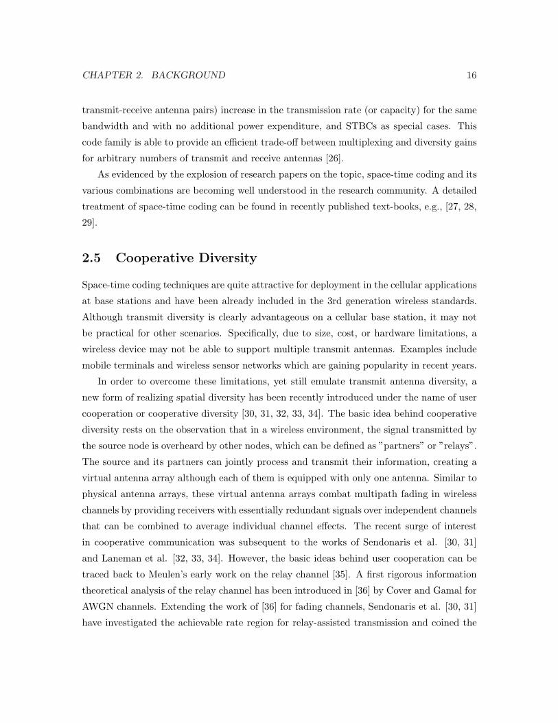
CHAPTER 2. BACKGROUND 17
Figure 2.2: Relay assisted transmission.
term ”user cooperation”.
In an independent work by Laneman et al. [32, 33] it is demonstrated that full spatial
diversity can be achieved through user cooperation. Their proposed user cooperation pro-
tocol is built upon a two-phase transmission scheme. In the first phase (i.e., broadcasting
phase), the source broadcasts to the destination and relay terminals. In the second phase
(i.e., relaying phase), the relays transmit processed version of their received signals to the
destination using either orthogonal subchannels, i.e., repetition based cooperative diversity,
or the same subchannel, i.e., space-time coded cooperative diversity. The latter relies on
the implementation of conventional orthogonal space-time block coding [15] in a distributed
fashion among the relay nodes.
Two main relaying techniques are studied in [32]: AF and Decode-and-Forward (DF).
In DF relaying, the relay node fully decodes, re-encodes and re-transmits the source node’s
message. In AF relaying, the relay retransmits a scaled version of the received signal
without any attempt to decode it. AF relaying can be furthered categorized based on the
availability of CSI at the relay terminal. In CSI-assisted AF scheme [32], the relay uses
instantaneous CSI of the source to relay (S → R) link to scale its received noisy signal
before re-transmission. This ensures that the same output power is maintained for each
CHAPTER 2. BACKGROUND 18
realization. On the hand, the ”blind” AF scheme does not have access to CSI and employs
fixed power constraint. This ensures that an average output power is maintained, but allows
for the instantaneous output power to be much larger than the average. Although blind AF
is not expected to perform as well as CSI-assisted AF relaying, the elimination of channel
estimation at the relay terminal promises low complexity and makes it attractive from a
practical point of view.
Another classification for relaying is also proposed in [32]. In the so-called ”fixed”
relaying, the relay always forwards the message that it receives from the source. The
performance of fixed DF relaying is limited by direct transmission between the source and
relay. An alternative to fixed relaying is ”selection” relaying (SR) which is, in nature,
adaptive to the channel conditions. In this type of relaying, the source reverts to non-
cooperation mode at times when the measured instantaneous SNR falls below a certain
threshold and continues its own direct transmission to the destination. The work in [37, 38]
can be considered as a systematic realization of such adaptive relaying through powerful
channel coding techniques. In so-called ”coded cooperation” of [37, 38], Hunter et al. realize
the concept of user cooperation through the distributed implementation of existing channel
coding methods such as convolutional and turbo codes. The basic idea is that each user
tries to transmit incremental redundancy for its partner. Whenever that is not possible,
the users automatically revert to a non-cooperative mode.
The user cooperation protocol proposed by Laneman et al. in [34] effectively implements
transmit diversity in a distributed manner. In [39], Nabar et al. establish a unified frame-
work of cooperation protocols for single-relay wireless networks. They quantify achievable
performance gains for distributed schemes in an analogy to conventional co-located multi-
antenna configurations. Specifically, they consider three (time-division multiple access)
TDMA-based protocols named Protocol I, Protocol II, and Protocol III which correspond to
traditional MIMO (multi-input-multi-output), SIMO (single-input-multi-output) and MISO
(multi-input -single-output) schemes, respectively (Table 1.1). In the following, we describe
these cooperation protocols which will be also a main focus of our work.
• Protocol I: During the first time slot, the source terminal communicates with the
relay and destination. During the second time slot, both the relay and source ter-
minals communicate with the destination terminal. This protocol realizes maximum
degrees of broadcasting and receive collision. In an independent work by Azarian et

CHAPTER 2. BACKGROUND 19
al. [40], it has been demonstrated that this protocol is optimum in terms of diversity-
multiplexing tradeoff. Protocol I is referred as ”non-orthogonal amplify and forward
(NAF) protocol” in [40].
• Protocol II: The source terminal communicates with the relay and destination ter-
minals in first time slot. In the second time slot, only the relay terminal communicates
with the destination. This protocol realizes a maximum degree of broadcasting and
exhibits no receive collision. This is the same cooperation protocol proposed by Lane-
man et al. in [32].
• Protocol III: This is essentially similar to Protocol I except that the destination
terminal does not receive from the source during the first time slot. This protocol
does not implement broadcasting but realizes receive collision.
Table 2.1: Cooperation protocols for single-relay networks.XXXXXXXXXXXProtocol
TerminalProtocol I Protocol II Protocol III
Time 1 Time 2 Time 1 Time 2 Time 1 Time 2Source • • • − • •Relay ◦ • ◦ • ◦ •
Destination ◦ ◦ ◦ ◦ − ◦
•: Transmitting, ◦: Receiving, −: Idle
2.6 Orthogonal frequency division multiplexing
The goal for people to have access to the capabilities of the global network at any time,
irrespective of the mobility and location, has become increasingly achievable, thanks to the
tremendous growth in wireless communication over the last two decades [41]. Moreover,
the increasing demand for wireless multimedia and interactive Internet services has led to
intensive research efforts on high speed data transmission. Unfortunately, unlike wireline
communication, there are crucial obstacles to wireless communications. Firstly, the radio
spectrum resources are very limited and expensive. Secondly, due to the harsh wireless en-
vironment, signals may undergo rapid fluctuations caused by multipath propagation when
CHAPTER 2. BACKGROUND 20
going through wireless channels [42, 7]. Therefore, the most desirable communication tech-
niques in this era, are those to improve the quality and spectral efficiency of the wireless
communication links.
A key challenge for high-speed broadband applications is the dispersive nature of frequency-
selective fading channels, which causes the so-called intersymbol interference (ISI), leading
to performance degradation.
To mitigate the ISI phenomenon, OFDM was proposed as an anti-multipath multicarrier
modulation scheme. OFDM is a multicarrier technique in which the transmitted bitstream
is divided into many different substreams and sent over many different subchannels, which
are orthogonal under ideal propagation conditions. The data rate on each of the subchannels
is much less than the total data rate, and the corresponding subchannel bandwidth is much
less than the total system bandwidth. The number of substreams is chosen to ensure that
each subchannel has a bandwidth less than the coherence bandwidth of the channel, so that
the subchannels experience relatively flat fading. This implementation, makes the ISI on
each subchannel small [43]. Note that the channel affects only the phase and amplitude of
the subcarrier and therefore, equalizing each subcarrier’s phase and gain, will compensate
for the frequency selective fading.
In order to generate the multiple subcarriers, the inverse fast Fourier transform (IFFT)
is performed at the transmitter side on blocks of M data symbols. Note that the fast
Fourier transform (FFT) block length M is at least 4-10 times longer than the maximum
impulse response span, mainly to minimize the fraction of overhead due to the insertion of
the cyclic prefix (CP) at the beginning of each block. Cyclic prefix is the repetition of the
last data symbols in a block and it serves two goals [44]: firstly, it prevents contamination
of a block by ISI from previous blocks. secondly, it makes the received block appear to be
periodic with period M . Note that the periodicity of the received block, produces circular
convolution, which is essential to the proper functioning of FFT.
2.7 Single-carrier frequency domain equalization
An SC system transmits a modulated single carrier at a high symbol rate and is basically
the frequency domain analog of what is done by conventional linear time domain equalizers.
Note that FDE is performed on a block of data at a time, where the operations on this block
involve an efficient FFT operation and a simple channel inversion operation, that makes it
CHAPTER 2. BACKGROUND 21
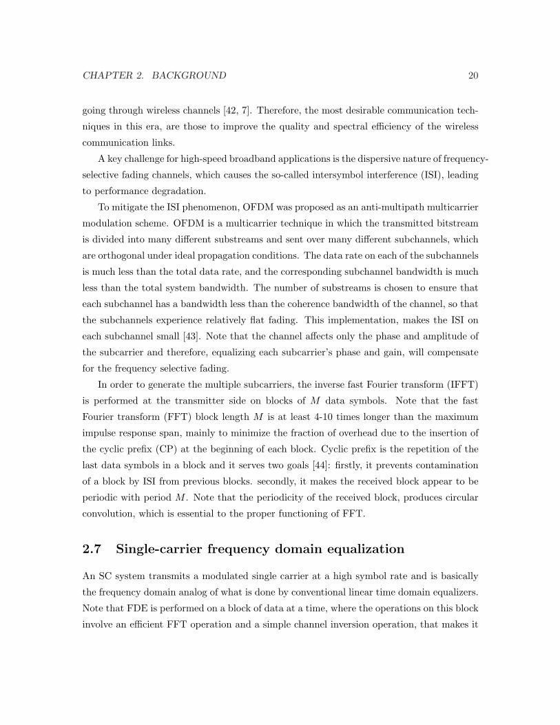
Figure 2.3: OFDM and SC-FDE– signal processing similarities and differences.
computationally simpler than the corresponding TD equalization, for channels with severe
delay spreads. Therefore, the SC system with FDE (SC-FDE) has essentially the same
performance and low complexity as OFDM, when combined with FFT processing and the
use of cyclic prefixing [45].
2.8 Summary
This chapter has covered different areas of wireless communication, knowledge of which is
essential to the rest of the thesis. These subjects include diversity techniques for fading
channels, transmit diversity techniques, space-time coding, cooperative diversity, multicar-
rier modulation techniques, OFDM, SC-FDE, and SC-STBC-FDE.
Chapter 3
A New Detection Scheme for
Zero-Padded OFDM
3.1 Introduction
Recently, ZP-OFDM has been proposed as an alternative solution to coded-OFDM, which
often incurs high decoding complexity. Various ZP-OFDM receivers have been proposed in
the literature, trading off performance with complexity. In this chapter, we propose a novel
low-complexity receiver for ZP-OFDM transmissions. We demonstrate that the proposed
receiver brings a significant complexity reduction in the receiver design, while outperforming
conventional MMSE-ZP-OFDM.
3.2 Overview
The growing demand for high data rate services for wireless multimedia and internet services
has lead to intensive research efforts on high speed data transmission. A key challenge for
high-speed broadband applications is the dispersive nature of frequency-selective fading
channels, which causes the so-called ISI leading to an inevitable performance degradation.
An efficient approach to mitigate ISI is the use of OFDM which converts the ISI channel
with AWGN into parallel ISI-free subchannels by implementing IFFT at the transmitter and
FFT at the receiver side [46]. It has been shown that OFDM is an attractive equalization
scheme for digital audio/video broadcasting (DAB/DVB) [47], and it has successfully been
applied to high-speed modems over digital subscriber lines (DSL) [48]. Recently, it has also
22
CHAPTER 3. A NEW DETECTION SCHEME FOR ZERO-PADDED OFDM 23
been proposed for broadband television systems and mobile wireless local area networks
such as IEEE802.11a and HIPERLAN/2 (HL2) standards [1].
The IFFT precoding at the transmitter side and insertion of CP enable OFDM with very
simple equalization of frequency-selective finite impulse response (FIR) channels. To avoid
InterBlock Interfernce (IBI) between successive FFT processed blocks, the CP is discarded
and the truncated blocks are FFT processed so that the frequency-selective channels are
converted into parallel flat-faded independent subchannels. In this way, the linear chan-
nel convolution is converted into circular convolution and the receiver complexity both in
equalization and the symbol decoding stages is reduced [49]. However, since each symbol is
transmitted over a single flat subchannel, the multipath diversity is lost along with the fact
there is no guarantee for symbol delectability when channel nulls occur in the subchannels.
As an additional counter-measure, coded OFDM (C-OFDM), which is fading resilient, has
been adopted in many standards [50]. Trellis-coded modulation (TCM) [51] and convolu-
tional codes [52, 53] are typical choices for error-control codes. Interleaving together with
TCM enjoys low complexity Viterbi decoding while enabling a better trade off between
bandwidth and efficiency. However, designing systems that achieve diversity gain equal to
code length is difficult considering the standard design paradigms for TCM. Linear constel-
lation precoded OFDM (LCP-OFDM) was further proposed in [54] to improve performance
over fading channels, where a real orthogonal precoder is applied to maximize the minimum
product distance [55, 56] and channel cutoff rate [57], while maintaining the transmission
rate and guaranteeing the symbol recovery. Subcarrier grouping was proposed in [54] to
enable the maximum possible diversity and coding gain. However, the LCP that is used
within each subset of subcarriers is in general complex.
To ensure symbol recovery regardless of channel nulls, ZP of multicarrier transmission
has been proposed to replace the generally non-zero CP. Unlike CP-OFDM, ZP-OFDM
guarantees symbol recovery and FIR equalization of FIR channels. Specifically, the zero
symbols are appended after the IFFT processed information symbols. In such way, the
single FFT required by CP-OFDM is replaced by FIR filtering in ZP-OFDM which adds to
the receiver complexity. To trade-off BER performance for extra savings in complexity, two
low complexity equalizers for ZP-OFDM are derived in [1]. Both schemes are developed
based on the circularity of channel matrix while reducing complexity by avoiding inversion
of a channel dependent matrix. However, the BER performance of the two sub-optimal
receivers proposed in [1] is not as good as MMSE-ZP-OFDM.

CHAPTER 3. A NEW DETECTION SCHEME FOR ZERO-PADDED OFDM 24
In this chapter, we propose a novel reduced complexity receiver design for ZP-OFDM
transmissions that not only outperforms MMSE-ZP-OFDM, but also uses low-complexity
computational methods that bring a significant power saving to the proposed receiver. This
makes it a strong candidate for WSNs which are characterized by small and low-power
devices. We show that linear processing collects both multipath and spatial diversity gains,
leading to significant improvement in performance, while maintaining low complexity.
3.3 System Model
We consider a single transmit single receive antenna system over a frequency-selective fad-
ing wireless channel. The (channel impulse response) CIR of the jth information block
is modeled as an FIR filter with coefficients hj =[hj [0], ..., hj [L]
]T, where L denotes the
corresponding channel memory length. The random vectors hj are assumed to be inde-
pendent zero-mean complex Gaussian with two choices of power delay profile: uniform
power delay profile with variance 1/ (L + 1); and exponentially decaying power-delay pro-
file θ(τk) = Ce−τk/τrms with delays τk that are uniformly and independently distributed
[58].
The jth M × 1 information block xjM is padded by D trailing zeros and IFFT precoded
by the IFFT matrix to yield the time-domain block vector xjzp
xjzp = Qzpx
jM , (3.1)
where
Qzp = [QM0D×M ]H . (3.2)
Therefore, the received block symbol is given by
rjzp = HQzpx
jM + HIBIQzpx
j−1M + nj
N , (3.3)
where N = M + D; H is the N ×N lower triangular Toeplitz filtering matrix with its first
column being[
hj [0], ..., hj [L] 0, ..., 0]T
; HIBI is the N × N upper triangular Toeplitz
filtering matrix that captures the (inter block interference) IBI, with its first row being[0, ..., 0 hj [0], ..., hj [L]
]; and nj
N denotes the AWGN noise. Having HIBIQzp = 0, the
all-zero 0D×M matrix plays the key role in ZP-OFDM by eliminating the IBI. Having the H
CHAPTER 3. A NEW DETECTION SCHEME FOR ZERO-PADDED OFDM 25
matrix partitioned between its first M and last D columns as H = [H0,Hzp], the received
block symbol will be given by
rjzp = HQzpx
jM + nj
N = H0QHMxj
M + njN . (3.4)
The N × M submatrix H0, which corresponds to the first M columns of H, is Toeplitz
and is guaranteed to be invertible, which assures symbol recovery regardless of channel zero
locations. In this case, owing to its channel-irrespective symbol delectability property, ZP-
OFDM is able to exploit fully the underlying multipath diversity [46]. Assuming variance
σ2x = 1 for the symbols, the MMSE equalizer for additive white Gaussian noise of variance
σ2n is given by [1]
Gmmse = QMHH0 (σ2
nIN + H0HH0 )−1. (3.5)
It should be emphasized that channel inversion of an N ×N matrix is costly to be precom-
puted due to its dependence on the channel. This brings about an extra implementation
cost for the MMSE-ZP-OFDM receiver. To overcome this limitation, our proposed scheme
targets practical ZP-OFDM receiver that exploits full multipath diversity.
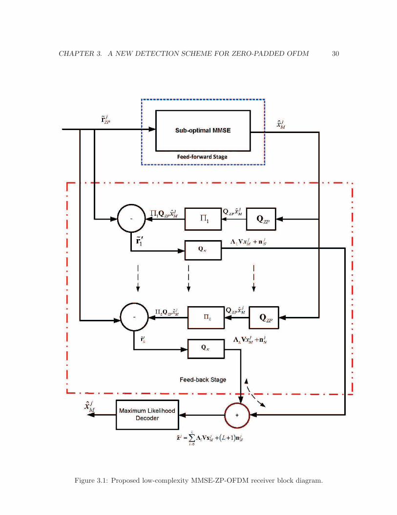
3.4 Reduced complexity MMSE-based receiver
The proposed receiver illustrated in Fig. 3.1 given in page 33, includes a suboptimal chan-
nel independent MMSE equalizer in the feed forward stage, followed by linear processing
operations in the feed-back stage. Specifically, the feed forward stage exploits the circulant
structure of the channel matrices,
H′ = QΛQH , (3.6)
where H′ is an N × N circulant matrix with entries [H′]k,l = h((k − l) mod N); Λ is a
diagonal matrix whose (n, n) element is equal to the nth discrete Fourier transform (DFT)
coefficient of h. Owing to the trailing zeros, the last D columns of H in (3.4) do not affect
the received block. Thus, the Toeplitz matrix H can be replaced by the N × N circulant
matrix H′ and (3.4) can be written as
rjzp = HQzpx
jM + nj
N = H′QzpxjM + nj
N . (3.7)
CHAPTER 3. A NEW DETECTION SCHEME FOR ZERO-PADDED OFDM 26
The H′ matrix takes advantage of FFT to yield a set of flat fading channels that can be
equalized easily. The ZP-OFDM receiver output will be
rjN = QNH′Qzpx
jM + nj
N = QNH′QHNQNQzpx
jM + nj
N = ΛVxjM + nj
N , (3.8)
where
V = QNQzp. (3.9)
After applying the N -point FFT QN to rjzp, the suboptimal MMSE-ZP-OFDM receiver in
the feed forward stage is formed in two steps. First, following [1], we obtain an MMSE
estimator of yjN = Vxj
M using
yjN = E[yj
N (rjN )
H].E−1[rj
N (rjN )
H] = VVHΛH [σ2
nI + ΛVVHΛH ]−1
. (3.10)
Assuming that VVH ≈ (P/N)I, (3.10) can be further simplified to
yjN = ΛH [(N/P )σ2
nI + ΛΛH ]−1. (3.11)
The resulting data streams detected from (3.11) are fed into a minimum Euclidean distance
decoder, yielding xjM , i.e., a decoded version of the transmitted symbols. The decoded sig-
nals are then fed into the feed-back stage, which is responsible for exploiting the underlying
multipath diversity. Specifically, consider the generation of the matrix Πl, l = 0, 1, 2, ..., L,
as follows:
[Πl]p,q =
0 p− q mod N = l
[H′]p,q p− q mod N 6= l, (3.12)
where 1 ≤ p, q ≤ N, then, (3.7) can be re-written as
r′l = rjzp −ΠlQzpx
jM . (3.13)
Under the high SNR assumption, we can safely assume that xjM ≈ xj
M . Therefore, we can
write (3.13) as follows:
r′l = HlQzpxjM + nj
N , (3.14)

CHAPTER 3. A NEW DETECTION SCHEME FOR ZERO-PADDED OFDM 27
where
[Hl]p,q =
[H′]p,q p− q mod N = l
0 p− q mod N 6= l. (3.15)
After taking the FFT of (3.14) we have:
zjl = QNHlQzpx
jM + nj
N = QNHlQHNQNQzpx
jM + nj
N = ΛlVxjM + nj
N , (3.16)
where Hl = QΛlQH ; Λl is a diagonal matrix whose nth element is equal to the DFT
coefficient of hjl = [ 0...0 hj [l] 0...0 ]. Interestingly, the frequency selective channels
are now converted in to parallel independent frequency flat channels. The signals zjl , l =
0, 1, ..., L, can now be combined, resulting in
zj =L∑
l=0
ΛlVxjM + (L + 1)nj
N . (3.17)
The signal in (3.17) is then processed by Λ† and V† where Λ =L∑
l=0
Λl and fed into a
maximum likelihood decoder to recover the transmitted symbols. It is observed from (3.17)
that the maximum achievable diversity order is given by L + 1. This illustrates that our
proposed receiver is able to fully exploit the underlying spatial and multipath diversity gains
relying on simple linear processing operations only.
3.5 Computational Complexity Analysis
In this section, we focus on the computational complexity of the proposed receiver compared
to the conventional MMSE-ZP-OFDM receiver. The computational complexity is measured
based on the number of the complex multiplications and complex divisions. Since complex
divisions can be implemented in various different ways, we did not decompose them into
complex multiplication. The overall computational complexity for the proposed receiver
and the conventional MMSE-ZP-OFDM receiver are summarized in Table 3.1 for the case
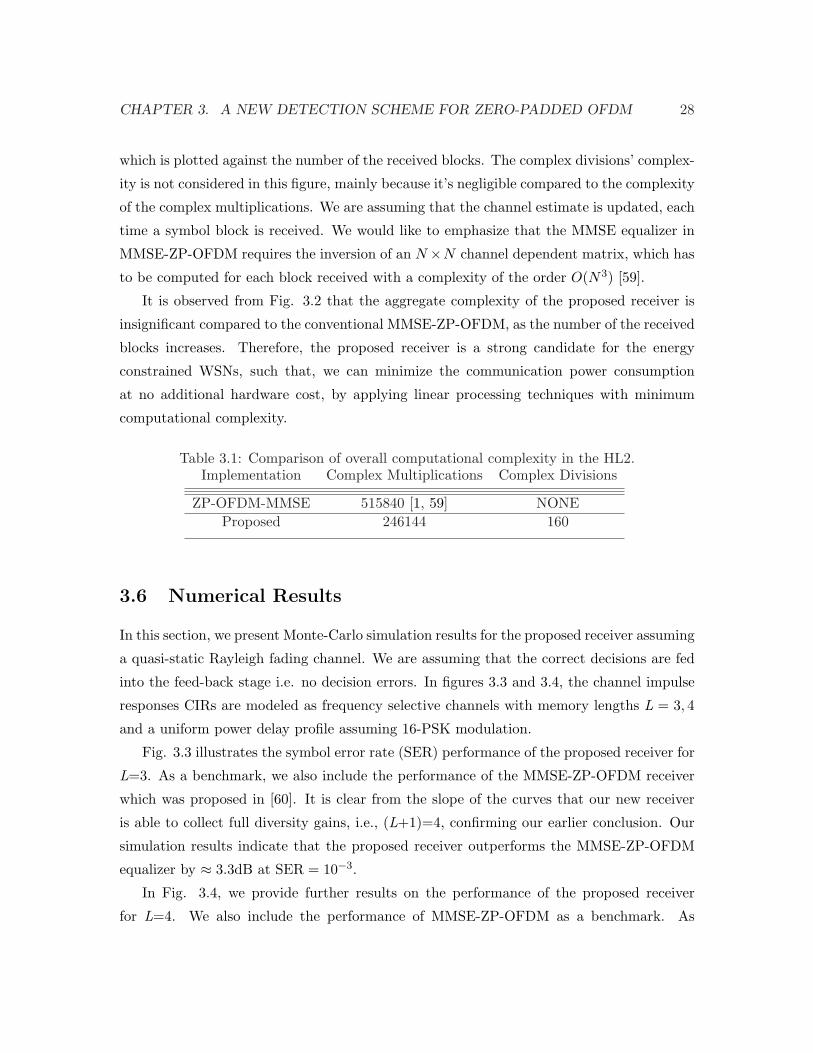
of HL2 (M=64 and N=80).
The computational complexity of the proposed receiver versus the MMSE-ZP-OFDM
receiver in terms of the number of the complex multiplications, is illustrated in Fig. 3.2,
CHAPTER 3. A NEW DETECTION SCHEME FOR ZERO-PADDED OFDM 28
which is plotted against the number of the received blocks. The complex divisions’ complex-
ity is not considered in this figure, mainly because it’s negligible compared to the complexity
of the complex multiplications. We are assuming that the channel estimate is updated, each
time a symbol block is received. We would like to emphasize that the MMSE equalizer in
MMSE-ZP-OFDM requires the inversion of an N×N channel dependent matrix, which has
to be computed for each block received with a complexity of the order O(N3) [59].
It is observed from Fig. 3.2 that the aggregate complexity of the proposed receiver is
insignificant compared to the conventional MMSE-ZP-OFDM, as the number of the received
blocks increases. Therefore, the proposed receiver is a strong candidate for the energy
constrained WSNs, such that, we can minimize the communication power consumption
at no additional hardware cost, by applying linear processing techniques with minimum
computational complexity.
Table 3.1: Comparison of overall computational complexity in the HL2.Implementation Complex Multiplications Complex Divisions
ZP-OFDM-MMSE 515840 [1, 59] NONEProposed 246144 160
3.6 Numerical Results
In this section, we present Monte-Carlo simulation results for the proposed receiver assuming
a quasi-static Rayleigh fading channel. We are assuming that the correct decisions are fed
into the feed-back stage i.e. no decision errors. In figures 3.3 and 3.4, the channel impulse
responses CIRs are modeled as frequency selective channels with memory lengths L = 3, 4
and a uniform power delay profile assuming 16-PSK modulation.
Fig. 3.3 illustrates the symbol error rate (SER) performance of the proposed receiver for
L=3. As a benchmark, we also include the performance of the MMSE-ZP-OFDM receiver
which was proposed in [60]. It is clear from the slope of the curves that our new receiver
is able to collect full diversity gains, i.e., (L+1)=4, confirming our earlier conclusion. Our
simulation results indicate that the proposed receiver outperforms the MMSE-ZP-OFDM
equalizer by ≈ 3.3dB at SER = 10−3.
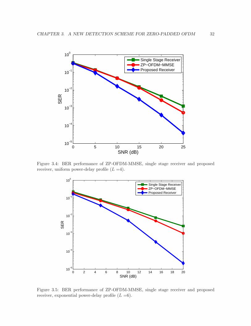
In Fig. 3.4, we provide further results on the performance of the proposed receiver
for L=4. We also include the performance of MMSE-ZP-OFDM as a benchmark. As

CHAPTER 3. A NEW DETECTION SCHEME FOR ZERO-PADDED OFDM 29
can be observed from the slope of the curve, the proposed receiver is able to collect full
diversity gains, i.e., (L+1)=5. Our results indicate that the proposed receiver outperforms
the MMSE-ZP-OFDM equalizer by 4.5dB at SER = 10−3.
In Fig. 3.5 and Fig. 3.6, the SER performance of the proposed receiver for L=6, 7 are
presented with exponential power-delay profile and 16 PSK modulation. In Fig. 3.5 our
results indicate that the proposed receiver outperforms the MMSE-ZP-OFDM equalizer by
8dB at SER = 10−3. This performance improvement is 8dB for Fig. 3.6 at SER = 10−3.
These results assure of the proposed receiver’s SER ourperformance compared to MMSE-
ZP-OFDM, for different power delay profile scenarios. Interestingly, it observed from Figs.
3.3, 3.4, 3.5 and 3.6 that performance improvement of the proposed receiver, in comparison
to the benchmark, increases as L increases.
3.7 Summary
We propose a novel reduced-complexity MMSE-based receiver for ZP-OFDM systems. We
show that, by incorporating linear processing techniques, our MMSE-based receiver is able
to collect full antenna and multipath diversity gains. Simulation results demonstrate that
our proposed receiver outperforms the conventional MMSE-ZP-OFDM receiver, while pro-
viding much less complexity by avoiding channel dependent matrix inversion. By using
linear processing techniques that require minimum computational complexity, the commu-
nication power is minimized at no additional hardware cost which makes the proposed
receiver a strong candidate for the energy constrained WSNs.
CHAPTER 3. A NEW DETECTION SCHEME FOR ZERO-PADDED OFDM 30
Figure 3.1: Proposed low-complexity MMSE-ZP-OFDM receiver block diagram.

CHAPTER 3. A NEW DETECTION SCHEME FOR ZERO-PADDED OFDM 31
1 2 3 4 50
0.5
1
1.5
2
2.5
3x 10
6
Blocks
Num
ber
of C
ompl
ex M
ultip
licat
ions
ZP−OFDM−MMSEProposed Receiver
Figure 3.2: Computational complexity of the proposed receiver compared to ZP-OFDM-MMSE.
0 2 4 6 8 10 12 14 16 18 2010
−4
10−3
10−2
10−1
100
SNR (dB)
SE
R
ZP−OFDM−MMSESingle Stage ReceiverProposed Receiver
Figure 3.3: BER performance of ZP-OFDM-MMSE, single stage receiver and proposedreceiver, uniform power-delay profile (L =3).
CHAPTER 3. A NEW DETECTION SCHEME FOR ZERO-PADDED OFDM 32
0 5 10 15 20 2510
−5
10−4
10−3
10−2
10−1
100
SNR (dB)
SE
R
Single Stage ReceiverZP−OFDM−MMSEProposed Receiver
Figure 3.4: BER performance of ZP-OFDM-MMSE, single stage receiver and proposedreceiver, uniform power-delay profile (L =4).
0 2 4 6 8 10 12 14 16 18 2010
−5
10−4
10−3
10−2
10−1
100
SNR (dB)
SE
R
Single Stage ReceiverZP−OFDM−MMSEProposed Receiver
Figure 3.5: BER performance of ZP-OFDM-MMSE, single stage receiver and proposedreceiver, exponential power-delay profile (L =6).

CHAPTER 3. A NEW DETECTION SCHEME FOR ZERO-PADDED OFDM 33
0 2 4 6 8 10 12 14 16 18 2010
−5
10−4
10−3
10−2
10−1
100
SNR (dB)
SE
R
Single Stage ReceiverZP−OFDM−MMSEProposed Receiver
Figure 3.6: BER performance of ZP-OFDM-MMSE, single stage receiver and proposedreceiver, exponential power-delay profile (L =7).

Chapter 4
MMSE-Based Receiver Design for
Single-Carrier Frequency Domain
Equalization
4.1 Introduction
In this chapter, we propose an efficient receiver design for SC-FDE for relay-assisted trans-
mission scenario over frequency selective channels. Building upon our earlier work [5], we
propose a novel MMSE-based receiver design tailored to broadband cooperative networks.
We show that our MMSE-based receiver is able to collect full antenna and multipath di-
versity gains. Specifically, under the assumption of perfect power control and high SNR
for the underlying links and assuming either of S → R or R → D links to be frequency
selective Rician fading, our performance analysis demonstrates that the proposed receiver
is able to achieve a maximum diversity order of min(LSR, LRD) + LSD + 2, where LSR,
LRD, and LSD are the channel memory lengths for S → R, R → D, and S → D links,
respectively. Complexity analysis and simulation results demonstrate that our proposed
receiver outperforms the conventional cooperative MMSE-SC-FDE receiver by performing
close to MFB, while providing minimal computational complexity.
34

CHAPTER 4. MMSE-BASED RECEIVER DESIGN FOR SC-FDE 35
4.2 System Model
A single-relay assisted cooperative communication scenario is considered. All terminals
are equipped with single transmit and receive antennas. Any linear modulation technique
such as QAM or PSK modulation can be used. We assume AF relaying and adopt the
user cooperation protocol proposed by Nabar et al. [39]. Specifically, the source terminal
communicates with the relay terminal during the first signaling interval. There is no trans-
mission from source-to-destination within this period. In the second signaling interval, both
the relay and source terminals communicate with the destination terminal.
The CIRs for S → R, S → D and R → D links for the jth transmission block
are given by hjSR =
[hj
SR[0], ..., hjSR[LSR]
]T, hj
RD =[hj
SD[0], ..., hjSD[LSD]
]Tand hj
SD =[hj
RD[0], ..., hjRD[LRD]
]T, respectively, where LSR, LRD and LSD denote the corresponding
channel memory lengths. The S → R link is assumed to be frequency selective Rician fading,
while the random vectors hjRD and hj
SD, are assumed to be independent zero-mean complex
Gaussian with power delay profile vectors denoted by vRD = [σ2RD(0), ..., σ2
RD(LRD)] and
vSD = [σ2SD(0), ..., σ2
SD(LSD)] that are normalized such that∑LRD
lRD=0 σ2RD (lRD) = 1 and
∑LSDlSD=0 σ2
SD (lSD) = 1. For the sake of presentation simplicity, the symmetrical scenario, in
which the R → D link is considered to be frequency selective Rician fading is omitted here.
In here we are assuming either of S → R or R → D to be frequncy selective Rician fading
based on the assumption that either of source terminal and relay terminal, or relay terminal
and the destination are close enough, so that the LOS path exists. The CIRs are assumed
to be constant over two consecutive blocks and vary independently every two blocks.
Information symbols are first parsed to two streams of M×1 blocks xji , i = 1, 2 and then
multiplied by a ZP matrix Ψ =[ITM ,0T
M×`
]T of size N×M , where ` = max (LSR, LSD, LRD)
and N is the frame length. The use of zero-padding as the precoding method in a single-
carrier transmission scenario ensures that the available multipath diversity is fully exploited.
To further remove inter-block interference and make the channel matrix circulant, a CP
with length ` is added between adjacent information blocks. Due to the adopted precoding
form, i.e., zero padding, we simply insert additional zeros at the start of the frame as CP.
The transmitted blocks for S → R and S → D links are generated by the encoding rule
dk+11 = −Jdk
2 , dk+12 = Jdk
1 k = 0, 2, 4, 6, ..., where di = Ψxi, i = 1, 2, is the zero-padded
information vector and J = PMN is a N ×N partial permutation matrix.

CHAPTER 4. MMSE-BASED RECEIVER DESIGN FOR SC-FDE 36
4.3 MMSE-based receiver for D-SC-STBC
In this section, we propose a novel, reduced-complexity MMSE-based receiver which enjoys a
remarkably simple decoding scheme. We show in the following section that the new proposed
receiver is able to collect full antenna and multipath diversity gains, while maintaining
minimal complexity.
The proposed receiver includes an MMSE equalizer, followed by linear processing op-
erations. Specifically, the first stage consists of the MMSE-D-STBC-SC scheme [3]. The
signal received at the relay terminal during the first signaling interval is
rjR =
√ESRHj
SRdj1 + nj
R, (4.1)
where njR is the additive white Gaussian noise vector with each entry having zero-mean and
variance of N0/2 per dimension. The relay terminal normalizes each entry of the received
signal [rjR]n, n = 1, 2, ..., N , by a factor of E
(|[rj
R]n|2)
= ESR + N0 to ensure unit average
energy and re-transmits the signal during the second time slot. After some mathematical
manipulations, the received signal at the destination terminal in the second time slot is
given by
rj =√
ERDESR
ESR + N0Hj
RDHjSRdj
1 +√
ESDHjSDdj
2 + nj . (4.2)
In (4.2), each entry of the effective noise term nj (conditioned on hRD) has zero mean and
a variance of ρN0 where ρ is defined by
ρ = 1 +ERD
ESR + N0
L3∑
m=0
|hRD (m)|2. (4.3)
In (4.1)-(4.2), HjSR, Hj
SD and HjRD are N × N circulant matrices with entries [Hj
i ]k,l =
hji ((k − l) mod N), i denotes SR, SD, RD, respectively. Finally, ESR, ESD and ERD are
the average energies available at the respective terminal which take into account possibly
different path loss and shadowing effects between the S → D and R → D links, respectively.
The destination terminal normalizes the received signal by a factor of√
ρ. This does not
affect the SNR, but simplifies the ensuing presentation [39]. After normalization, we obtain
rj =√
γ1HjRDHj
SRdj1 +
√γ2H
jSDdj
2 + nj , (4.4)
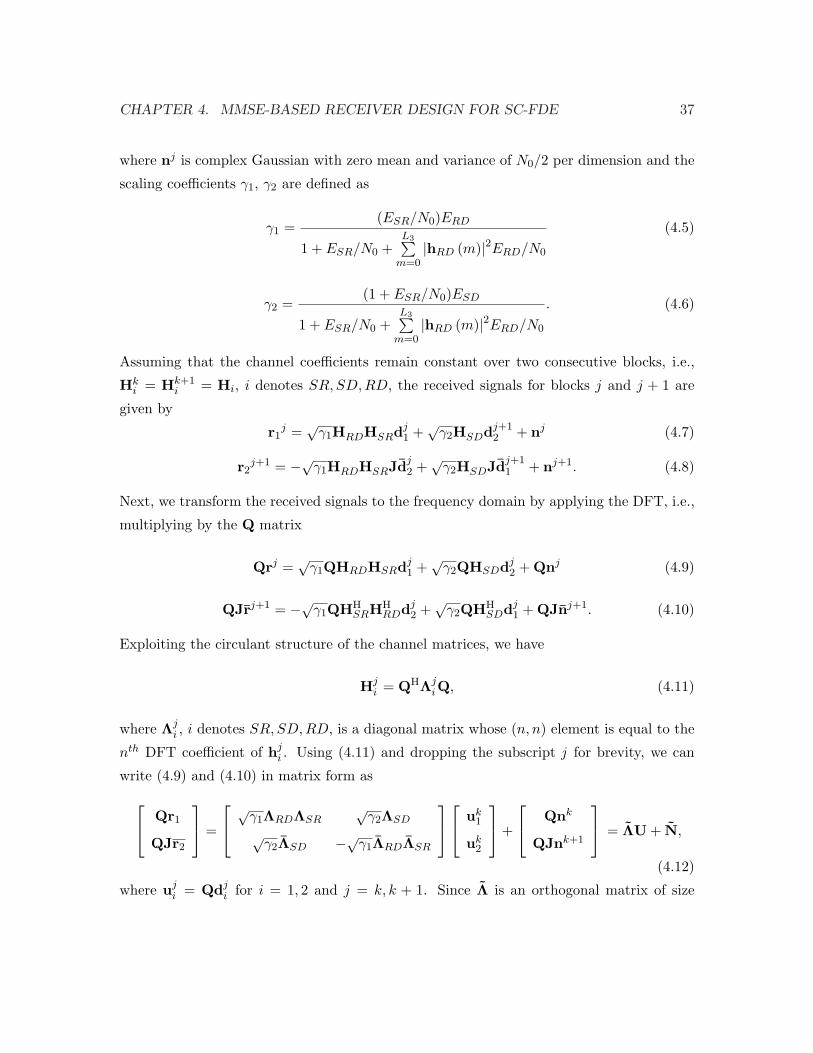
CHAPTER 4. MMSE-BASED RECEIVER DESIGN FOR SC-FDE 37
where nj is complex Gaussian with zero mean and variance of N0/2 per dimension and the
scaling coefficients γ1, γ2 are defined as
γ1 =(ESR/N0)ERD
1 + ESR/N0 +L3∑
m=0|hRD (m)|2ERD/N0
(4.5)
γ2 =(1 + ESR/N0)ESD
1 + ESR/N0 +L3∑
m=0|hRD (m)|2ERD/N0
. (4.6)
Assuming that the channel coefficients remain constant over two consecutive blocks, i.e.,
Hki = Hk+1
i = Hi, i denotes SR, SD,RD, the received signals for blocks j and j + 1 are
given by
r1j =
√γ1HRDHSRdj
1 +√
γ2HSDdj+12 + nj (4.7)
r2j+1 = −√γ1HRDHSRJdj
2 +√
γ2HSDJdj+11 + nj+1. (4.8)
Next, we transform the received signals to the frequency domain by applying the DFT, i.e.,
multiplying by the Q matrix
Qrj =√
γ1QHRDHSRdj1 +
√γ2QHSDdj
2 + Qnj (4.9)
QJrj+1 = −√γ1QHHSRHH
RDdj2 +
√γ2QHH
SDdj1 + QJnj+1. (4.10)
Exploiting the circulant structure of the channel matrices, we have
Hji = QHΛj
iQ, (4.11)
where Λji , i denotes SR, SD, RD, is a diagonal matrix whose (n, n) element is equal to the
nth DFT coefficient of hji . Using (4.11) and dropping the subscript j for brevity, we can
write (4.9) and (4.10) in matrix form as
Qr1
QJr2
=
√
γ1ΛRDΛSR√
γ2ΛSD
√γ2ΛSD −√γ1ΛRDΛSR
uk
1
uk2
+
Qnk
QJnk+1
= ΛU + N,
(4.12)
where uji = Qdj
i for i = 1, 2 and j = k, k + 1. Since Λ is an orthogonal matrix of size
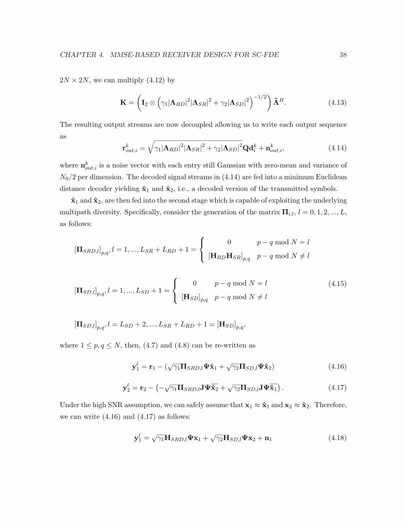
CHAPTER 4. MMSE-BASED RECEIVER DESIGN FOR SC-FDE 38
2N × 2N , we can multiply (4.12) by
K =(I2 ⊗
(γ1|ΛRD|2|ΛSR|2 + γ2|ΛSD|2
)−1/2)
ΛH . (4.13)
The resulting output streams are now decoupled allowing us to write each output sequence
as
rkout,i =
√γ1|ΛRD|2|ΛSR|2 + γ2|ΛSD|2Qdk
i + nkout,i, (4.14)
where nkout,i is a noise vector with each entry still Gaussian with zero-mean and variance of
N0/2 per dimension. The decoded signal streams in (4.14) are fed into a minimum Euclidean
distance decoder yielding x1 and x2, i.e., a decoded version of the transmitted symbols.
x1 and x2, are then fed into the second stage which is capable of exploiting the underlying
multipath diversity. Specifically, consider the generation of the matrix Πi,l, l = 0, 1, 2, ..., L,
as follows:
[ΠSRD,l]p,q, l = 1, ..., LSR + LRD + 1 =
0 p− q mod N = l
[HRDHSR]p,q p− q mod N 6= l
[ΠSD,l]p,q, l = 1, ..., LSD + 1 =
0 p− q mod N = l
[HSD]p,q p− q mod N 6= l
[ΠSD,l]p,q, l = LSD + 2, ..., LSR + LRD + 1 = [HSD]p,q,
(4.15)
where 1 ≤ p, q ≤ N, then, (4.7) and (4.8) can be re-written as
yl1 = r1 − (
√γ1ΠSRD,lΨx1 +
√γ2ΠSD,lΨx2) (4.16)
yl2 = r2 −
(−√γ1ΠSRD,lJΨx2 +√
γ2ΠSD,lJΨx1
). (4.17)
Under the high SNR assumption, we can safely assume that x1 ≈ x1 and x2 ≈ x2. Therefore,
we can write (4.16) and (4.17) as follows:
yl1 =
√γ1HSRD,lΨx1 +
√γ2HSD,lΨx2 + n1 (4.18)

CHAPTER 4. MMSE-BASED RECEIVER DESIGN FOR SC-FDE 39
yl2 = −√γ1HSRD,lJΨx2 +
√γ2HSD,lJΨx1 + n2, (4.19)
where ni (i=1,2) is complex Gaussian with zero mean and variance of N0/2 per dimension
and
[HSRD,l]p,q, l = 1, ..., LSR + LRD + 1 =
[HRDHSR]p,q p− q mod N = l
0 p− q mod N 6= l
[HSD,l]p,q, l = 1, ..., LSD + 1 =
[HSD]p,q p− q mod N = l
0 p− q mod N 6= l
[HSD,l]p,q, l = LSD + 2, ..., LSR + LRD + 1 = 0.
(4.20)
Conjugating Jyl2 and using the fact JHi,lJ = HH
i,l, we obtain
Jyl2 = −√γ1HH
SRD,lΨx2 +√
γ2HHSD,lΨx1 + Jn2. (4.21)
In matrix form, we can write (4.18) and (4.21) as
yl
1
Jyl2
=
√
γ1HSRD,l√
γ2HSD,l
√γ2HH
SD,l −√γ1HHSRD,l
︸ ︷︷ ︸Heq,l
Ψx1
Ψx2
+
n1
Jn2
. (4.22)
Multiplying (4.22) by
(I2 ⊗
(γ1|HSRD,l|2 + γ2|HSD,l|2
)−1/2)
HHeq,l. (4.23)
we observe that the output streams are decoupled (due to orthogonality of Heq,l), allowing
us to write
zli =
√γ1|HSRD,l|2 + γ2|HSD,l|2Ψxi + ni, (4.24)
where the noise term is still complex Gaussian with the variance of N0/2 per dimension.
Interestingly, the frequency selective channels are now converted in to parallel independent

CHAPTER 4. MMSE-BASED RECEIVER DESIGN FOR SC-FDE 40
frequency flat channels. The signals zli, l = 0, 1, ..., L, can now be combined, resulting in
zi =L∑
l=0
√γ1|HSRD,l|2 + γ2|HSD,l|2Ψxi + ni, (4.25)
where without loss of generality, L = LSR + LRD + 1 and ni is complex Gaussian with
variance of N ′0 = (L + 1)N0/2 per dimension. The signals in (4.25) are then fed into a
maximum likelihood decoder to recover the transmitted symbols.
4.4 Diversity Gain Analysis
Here, we investigate the achievable diversity gain for the proposed receiver through the
derivation of the PEP expression.
Defining the transmitted codeword vector and the erroneously-decoded codeword vector
as x and x, respectively, and applying the standard Chernoff bound, we obtain
P (x, x|hSR,hRD,hSD) ≤ exp(−d2(x, x)
4N ′0
), (4.26)
where d2(x, x) denotes the Euclidean distance between x and x. Following [3], the Euclidean
distance in (4.26) can be expressed as
d2(x, x) = γ1‖HRDHSRe1‖2 + γ2‖HSDe2‖2, (4.27)
where ei = di − di, i = 1, 2.
Having ‖Hi‖2 = NLi∑
li=0
(|hi(li)|)2 i = SR, SD , where N is the frame length, (4.27) can
be further simplified to
d2(x, x) ≈ γ1∑LRD
lRD=0hRD(lRD)2‖HSRe1‖2 + γ2‖HSDe2‖2
≈ γ1∑LSR
lSR=0hSR(lSR)2‖HRDe1‖2 + γ2‖HSDe2‖2
(4.28)

CHAPTER 4. MMSE-BASED RECEIVER DESIGN FOR SC-FDE 41
Introducing
<i =
[d]0 [d]1 · · · [d]N−1
[d]N−1 [d]0 · · · [d]N−2
...... · · · ...
[d]N−Li[d]N−Li+1 · · · [d]N−Li−1
(4.29)
and –<i = (<i − <i)(<i − <i)H , for i = 1, 2, (4.28) can be written as follows
d2(x, x) ≈ γ1
LRD∑lRD=0
hRD(lRD)2hTSR–<1(hT
SR)H + γ2hTSD–<2(hT
SD)H . (4.30)
Defining Θi = diag(vi), µi = Θi−1/2hi, and Ai = Θ1/2
i –<iΘ1/2i , i = SR, SD, we have
d2(x, x) ≈ γ1
LRD∑lRD=0
hRD(lRD)2µTSRASR(µT
SR)H + γ2µTSDASD(µT
SD)H , (4.31)
where Ai, i = SR, SD are Hermitian and full rank [3]. Therefore, there exists a unitary
matrix UAi such that UHAi
AiUAi = ∆i where ∆i is a diagonal matrix with elements equal
to the eigenvalues of Ai. Therefore, (4.31) can be expressed as
d2(x, x) ≈ γ1
LRD∑lRD=0
hRD(lRD)2βSR∆SRβHSR + γ2βSD∆SDβH
SD, (4.32)
where βi = µTi UAi , i = SR, SD. Thus, (4.32) can be further simplified to
d2(x, x) ≈ γ1
LRD∑
lRD=0
|hRD(lRD)|2LSR∑
lSR=0
λSR(lSR)|βSR(lSR)|2 + γ2
LSD∑
lSD=0
λSD(lSD)|βSD(lSD)|2,
(4.33)
where λSR(lSR)(λSD(lSD)) denote the lthSR
(lthSD
)eigenvalue of codeword difference matrixes
and βSR (βSD) are zero-mean complex Gaussian vectors with unit variance. Assuming
perfect power control and sufficiently large ESR/N0 > ESD/N0 values, the scaling factors
in (4.5) and (4.6) reduce to γ1 = γ2 = ESD. Then, we can write (6.33) as
d2(x, x) ≈ ESD
LRD∑
lRD=0
|hRD(lRD)|2LSR∑
lSR=0
λSR(lSR)|βSR(lSR)|2+ESD
LSD∑
lSD=0
λSD(lSD)|βSD(lSD)|2.
(4.34)
CHAPTER 4. MMSE-BASED RECEIVER DESIGN FOR SC-FDE 42
In the following, we will derive the PEP expression under two different scenarios:
Case I: LRD > LSR
First, we define the random variables Y2 =∑LSD
lSD=0 λSD(lSD)|βSD(lSD)|2 and Y1 = X1X2
with X1 =∑LRD
lRD=0 |hRD(lRD)|2 and X2 =∑LSR
lSR=0 λSR(lSR)|βSR(lSR)|2. Substituting (4.33)
in (4.26) and averaging the resulting expression with respect to Y1 and Y2, we obtain
P (x, x) ≤ EY1
[exp
(−ESD
4N ′0Y1
)]EY2
[exp
(−ESD
4N ′0Y2
)]
= ΦY1 (ω)|jω=−ESD
4N′0× ΦY2 (ω)|
jω=−ESD4N′0
,(4.35)
where ΦY1 (ω) and ΦY2 (ω) are the characteristic functions of Y1 and Y2 respectively. Since
the entries of |βSD| are Rayleigh distributed, ΦY2 (ω) is given as [61]
ΦY2(ω)|jω=−ESD
4N′0=
LSD∏
lSD=0
(1 +
ESD
4N ′0λSD(lSD)
)−1
. (4.36)
ΦY1 (ω) can be evaluated as [3]
ΦY 1(ω) =
∞∫
0
fX1(x1)ΦX2(ωx1)dx1, (4.37)
where fX1(x1), x1 ≥ 0 is the probability density function (pdf) of X1, and φX2(ωx1) is
the characteristic function of X2. Having X1 to be a chi squared random variable with
2(LRD + 1) degrees of freedom [3],
fX1(x1) =(LRD + 1)LRD+1
Γ(LRD + 1)xLRD
1 e−(LRD+1)x1 (4.38)
and φY1(ωx1) can be evaluated as [3]
φX2(ωx1) =LSR∏
lSR=0
[1 + n2
1 + n2 − ωλSR(lSR)x1e
n2ωλx11+n2−ωλx1
]. (4.39)

CHAPTER 4. MMSE-BASED RECEIVER DESIGN FOR SC-FDE 43
where n is the fading parameter. Having (4.38) and (4.39), (4.37) can be evaluated as
φY1(ω)|jω=
−ESD4N′0
=
=∫∞0
(LRD+1)LRD+1
Γ(LRD+1) xLRD1 e−(LRD+1)x1 ×∏LSR
lSR=0
1+n2
1+n2+ESD4N′0
λSR(lSR)x1
e
−n2 ESD4N′0
λSR(lSR)x1
1+n2+ESD4N′0
λSR(lSR)x1
= (LRD+1)LRD+1
Γ(LRD+1) e−(LRD+1)x1 ×∏LSRlSR=0
∫∞0
xLRD1 (1+n2)
1+n2+ESD4N′0
λSR(lSR)x1
e
−n2 ESD4N′0
λSR(lSR)x1
1+n2+ESD4N′0
λSR(lSR)x1
.
(4.40)
Assuming high SNR, i.e., ESD/4N ′0 À 1, (4.40) can be simplified as
φZ1(ω)|jω=
−ESD4N′0
= R(
ESD4N ′
0
)−(LSR+1)λ−(LSR+1)
× ∫∞0
x
LRD1∏LSR
lSR=0
1ESD4N′0
λSR(lSR)+
x11+n2
e−n2e−(LRD+1)x1
,
(4.41)
where R = (LRD+1)LRD+1
Γ(LRD+1) . After further simplification, (4.41) can be written as
φY1(ω)|jω=
−ESD4N′0
=(1 + n2)LSR+1
(LRD + 1)e−n2(LSR+1)
LRD − LSR×R
(ESD
4N ′0
)−(LSR+1)
λ−(LSR+1)Γ(LRD−LSR).
(4.42)
Substituting (4.42) and (4.36) in (4.35), we find the final PEP expression given as
P (x, x) ≤ (1+n2)LSR+1
(LRD+1)e−n2(LSR+1)
LRD−LSRR
(ESD4N ′
0
)−(LSR+1)
×λ−(LSR+1)Γ(LRD − LSR)∏LSD
lSD=0
(1 + ESD
4N ′0λSD(lSD)
)−1.
(4.43)
Case II: LSR > LRD
Noting that this case is similar to Case I with LSR and LRD interchanged, we consider the
random variable Z2 = X2Y2, with X2 =LSR∑
lSR=0
|hSR(lSR)|2 and Y2 =LRD∑
lRD=0
λRD(lRD)|hRD(lRD)|2.The characteristic function of Z2, φZ2 , can be evaluated as
φZ2(ω) =
∞∫
0
fX2(u)φY2(ωu)du. (4.44)
CHAPTER 4. MMSE-BASED RECEIVER DESIGN FOR SC-FDE 44
Using the integral form given in [62],
fX2(u) =(
(LSR+1+KR)LRD+1
1/(LSR+1)
) [(LSR+1+KR)
KR(1/(LSR+1))
]LSR/2× e
−[KR+
(LSR+1+KR)
1/(LSR+1)u]ILSR
[2√
KR(LSR+1+KR)1/(LSR+1) u
],
(4.45)
where KR =LSR∑
lSR=0
KlSR, and KlSR
is the Rician parameter on the lSRth tap. (4.44) can be
further simplified to
φZ2(ω) = c(c
KR)LSR/2e−k2
∞∫
0
uLSR/2e−cuILSR(2
√KRcu)×
LRD∏
lRD=0
11 + ESD
4N ′0λRD(lRD)u
,
(4.46)
where c = (LSR + 1 + KR) (LSR + 1) and ILSR(α) =(
α2
)LSR∞∑
k=0
(α2
4
)k1
k!Γ(k+LSR+1) . Using
the fact that∫∞0 yn−1e−aydy = a−uΓ(n), after some mathematical manipulations, (4.46)
yields
φZ2(ω) = [(LSR + 1)(LSR + 1 + KR)]LRD−LSR/2 × e−KR
(ESD4N ′
0
)−(LRD+1)
×∏LRDlRD=0 λRD(lRD)−1 ×
∞∑k=0
KRΓ(LSR+k−LRD)k!Γ(LSR+k+1) .
(4.47)
Substituting (4.47) and (4.36) in (4.35), we find the final PEP expression given as
P (x, x) ≤ [(LSR + 1)(LSR + 1 + KR)]LRD−LSR/2 × e−KR
(ESD4N ′
0
)−(LRD+1) LRD∏lRD=0
λRD(lRD)−1
×∞∑
k=0
KRΓ(LSR+k−LRD)k!Γ(LSR+k+1) ×
LSD∏lSD=0
(1 + ESD
4N ′0λSD(lSD)
)−1.
(4.48)
It is observed from (4.43) and (4.48) that the maximum achievable diversity order is given
by min(LSR, LRD) + LSD + 2. This is consistent with the results reported in [3].
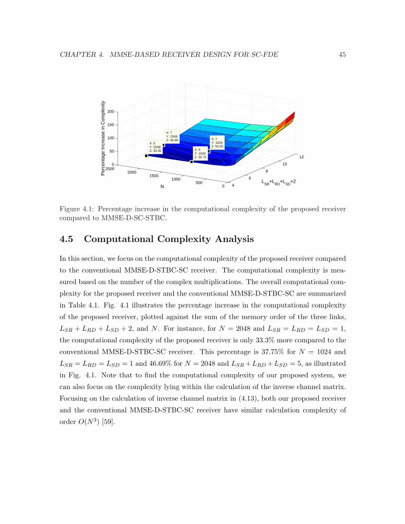
CHAPTER 4. MMSE-BASED RECEIVER DESIGN FOR SC-FDE 45
4
6
8
10
12
0500
10001500
20002500
0
50
100
150
200
LSR
+LRD
+LSD
+2
X: 7Y: 1024Z: 50.05
X: 5Y: 1024Z: 35.75
X: 7Y: 2048Z: 46.69
N
X: 5Y: 2048Z: 33.35
Per
cent
age
Incr
ease
in C
ompl
exity
Figure 4.1: Percentage increase in the computational complexity of the proposed receivercompared to MMSE-D-SC-STBC.
4.5 Computational Complexity Analysis
In this section, we focus on the computational complexity of the proposed receiver compared
to the conventional MMSE-D-STBC-SC receiver. The computational complexity is mea-
sured based on the number of the complex multiplications. The overall computational com-
plexity for the proposed receiver and the conventional MMSE-D-STBC-SC are summarized
in Table 4.1. Fig. 4.1 illustrates the percentage increase in the computational complexity
of the proposed receiver, plotted against the sum of the memory order of the three links,
LSR + LRD + LSD + 2, and N . For instance, for N = 2048 and LSR = LRD = LSD = 1,
the computational complexity of the proposed receiver is only 33.3% more compared to the
conventional MMSE-D-STBC-SC receiver. This percentage is 37.75% for N = 1024 and
LSR = LRD = LSD = 1 and 46.69% for N = 2048 and LSR +LRD +LSD = 5, as illustrated
in Fig. 4.1. Note that to find the computational complexity of our proposed system, we
can also focus on the complexity lying within the calculation of the inverse channel matrix.
Focusing on the calculation of inverse channel matrix in (4.13), both our proposed receiver
and the conventional MMSE-D-STBC-SC receiver have similar calculation complexity of
order O(N3) [59].
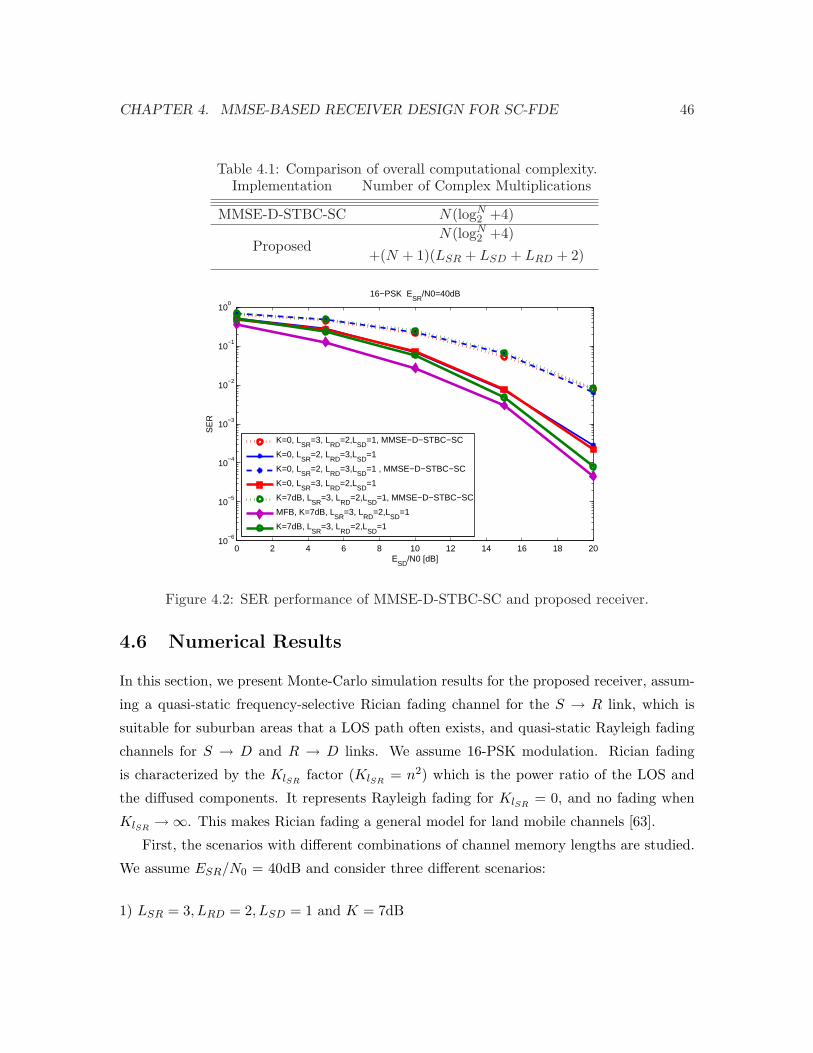
CHAPTER 4. MMSE-BASED RECEIVER DESIGN FOR SC-FDE 46
Table 4.1: Comparison of overall computational complexity.Implementation Number of Complex Multiplications
MMSE-D-STBC-SC N(logN2 +4)
ProposedN(logN
2 +4)+(N + 1)(LSR + LSD + LRD + 2)
0 2 4 6 8 10 12 14 16 18 2010
−6
10−5
10−4
10−3
10−2
10−1
100
ESD
/N0 [dB]
SE
R
16−PSK ESR
/N0=40dB
K=0, LSR
=3, LRD
=2,LSD
=1, MMSE−D−STBC−SC
K=0, LSR
=2, LRD
=3,LSD
=1
K=0, LSR
=2, LRD
=3,LSD
=1 , MMSE−D−STBC−SC
K=0, LSR
=3, LRD
=2,LSD
=1
K=7dB, LSR
=3, LRD
=2,LSD
=1, MMSE−D−STBC−SC
MFB, K=7dB, LSR
=3, LRD
=2,LSD
=1
K=7dB, LSR
=3, LRD
=2,LSD
=1
Figure 4.2: SER performance of MMSE-D-STBC-SC and proposed receiver.
4.6 Numerical Results
In this section, we present Monte-Carlo simulation results for the proposed receiver, assum-
ing a quasi-static frequency-selective Rician fading channel for the S → R link, which is
suitable for suburban areas that a LOS path often exists, and quasi-static Rayleigh fading
channels for S → D and R → D links. We assume 16-PSK modulation. Rician fading
is characterized by the KlSRfactor (KlSR
= n2) which is the power ratio of the LOS and
the diffused components. It represents Rayleigh fading for KlSR= 0, and no fading when
KlSR→∞. This makes Rician fading a general model for land mobile channels [63].
First, the scenarios with different combinations of channel memory lengths are studied.
We assume ESR/N0 = 40dB and consider three different scenarios:
1) LSR = 3, LRD = 2, LSD = 1 and K = 7dB

CHAPTER 4. MMSE-BASED RECEIVER DESIGN FOR SC-FDE 47
0 2 4 6 8 10 12 14 16 18 2010
−5
10−4
10−3
10−2
10−1
100
ESD
/N0 [dB]
SE
R
16 PSK ESR
/N0=40dB
K=7dB, LSR
=3, LRD
=1,LSD
=1
K=0, LSR
=3, LRD
=1,LSD
=1
K=0, LSR
=1, LRD
=3,LSD
=1
K=7dB, LSR
=3, LRD
=1,LSD
=1, MMSE−D−STBC−SC
K=0, LSR
=3, LRD
=1,LSD
=1, MMSE−D−STBC−SC
MFB, K=7dB, LSR
=3, LRD
=1,LSD
=1
Figure 4.3: SER performance of MMSE-D-STBC-SC and proposed receiver.
0 5 10 15 20 25
10−2
10−1
100
ESD
/N0 [dB]
SE
R
16−PSK , K=7 dB, LSR
=4, LSD
=LRD
=3
Proposed, E
SR/N0=20 dB
MMSE−D−SC−STBC, ESR
/N0=20 dB
Proposed, ESR
/N0=35 dB
MMSE−D−SC−STB, ESR
/N0=35 dB
Figure 4.4: SER performance of MMSE-D-STBC-SC and proposed receiver.
2) LSR = 3, LRD = 2, LSD = 1 and K = 0
3) LSR = 2, LRD = 3, LSD = 1 and K = 0
Note that we are choosing ESR/N0= 40dB for the sake of presentation. As long as
CHAPTER 4. MMSE-BASED RECEIVER DESIGN FOR SC-FDE 48
ESR/N0 À 25dB, its safe to assume that there is no error propagation from the first
stage to the feed-back stage.
In Fig. 4.2, Performance of MMSE-D-SC-STBC and the proposed receiver for each of
these scenarios is illustrated. As a benchmark, we also include MFB performance, which
doesn’t take ISI into account. It can be seen that identical SER performance is achieved by
interchanging the values of LSR and LRD, which confirms our previous observations from
PEP analysis. It is clear from the slope of the curves that our new receiver is able to collect
full diversity gains, i.e., min(LRD, LSR) + LSD + 2 = 5, confirming our earlier conclusion.
Our simulation results indicate that, for the first scenario, the proposed receiver outperforms
the MMSE-D-SC-STBC equalizer by ≈5.5dB at BER = 10−2. For the second scenario, the
proposed receiver outperforms the MMSE-D-SC-STBC receiver by ≈4.5dB at BER = 10−2.
The proposed receiver still has a degradation of 1dB compared to the MFB.
Secondly, we assume ESR/N0 = 40dB and consider the following cases in Fig. 4.3,
where performance of the following scenarios is analyzed for MMSE-D-SC-STBC and the
proposed receiver:
1) LSR = 3, LRD = 1, LSD = 1 and K=7dB
2) LSR = 3, LRD = 1, LSD = 1 and K=0dB
3) LSR = 1, LRD = 3, LSD = 1 and K=0dB
4) LSR = 1, LRD = 3, LSD = 1 and K=7dB
Note that similar SER performance is acheived while interchanging the values of LSR and
LRD. Our results indicate that for the first scenario, the proposed receiver outperforms the
MMSE-D-SC-STBC equalizer by 4.5dB at BER = 10−2. Having LSR +LRD +LSD +2 = 7,
the number of complex multiplications for the proposed receiver is 1095 while the MMSE-
D-STBC-SC receiver employs 640 complex multiplication. This extra cost gives ≈4.5dB
performance increase at SER = 10−2 for the proposed receiver. For the second scenario, the
proposed receiver outperforms the MMSE-D-SC-STBC receiver by ≈3dB at BER = 10−2.
The proposed receiver has a degradation of 2dB compared to the MFB.
In Fig. 4.4, we assume LSR = 4, LRD = LSD = 3 and K=7dB and study the per-
formance of the system for different ESR/N0 values. The performance of the proposed
receiver degrades as ESR/N0 decreases, which confirms our earlier observations. It can be

CHAPTER 4. MMSE-BASED RECEIVER DESIGN FOR SC-FDE 49
seen that at SER = 10−2, the proposed receiver working at ESR/N0=35dB outperforms its
counterpart working at ESR/N0=5dB by 15dB. Interestingly, it is observed from Figs. 4.2,
4.3 and 4.4 that performance improvement of the proposed receiver, in comparison to the
benchmark, increases as L increases, which comes at low additional cost.
4.7 Summary
We propose a novel reduced-complexity MMSE-based receiver for D-SC-STBC transmis-
sions. We show that our MMSE-based receiver is able to collect full antenna and multipath
diversity gains. We show that the computational complexity of our proposed system is
comparable to the conventional MMSE-D-SC-STBC receiver while collecting the maximum
achievable diversity order of min(LSR, LRD) + LSD + 2. Simulation results demonstrate
that our proposed receiver outperforms the conventional MMSE-D-SC-STBC receiver, while
maintaining low complexity tradeoff.
Chapter 5
Distributed Single-Carrier
Frequency Domain Equalization in
Multi-Relay Networks.
5.1 introduction
In this chapter, we investigate the performance of SC-FDE for D-STBC systems with
AF relaying over frequency-selective Rician fading channels. Our performance analysis
demonstrates that SC-FDE for DSTB is able to achieve a maximum diversity order ofR∑
i=1min(LSRi , LRiD) + R, where R is the number of participating relays, LSRi and LRiD are
the channel memory lengths for source to ith relay (S → Ri) link and ith relay to destination
(Ri → D) link, respectively. Simulation results are provided to corroborate the theoretical
analysis.
5.2 overview
A combination of STBC with SC-FDE for frequency-selective channels was presented in
[64]. Most of the current literature on SC-FDE is limited to point-to-point communication
systems. However, there have been recent results reported on FDE in the context of coop-
erative scenarios [3, 4]. Assuming the MLSD equalizers, D-STBC SC-FDE has been first
discussed in [3] as an extension of conventional STBC to cooperative systems. The results
50
CHAPTER 5. DSTBC SC-FDE FOR MULTI-RELAY NETWORKS 51
in [3], however, are restricted to a single-relay scenario with AF relaying over Rayleigh fad-
ing channels. The asymptotical PEP behavior for a large number of relays is analyzed in
[65, 66], but this analysis is restricted to frequency flat Rayleigh fading channels.
In this chapter, we extend the work in [3] to a multi-relay scenario. In particular, we drive
a PEP expression for D-SC-FDE-STBC over frequency-selective Rician fading channels and
show that the maximum achievable diversity order isR∑
i=1min(LSRi , LRiD) + R.
5.3 Transmission Model
We consider a multiple-relay assisted cooperative wireless communication system with a
single source (S), R half-duplex relay terminals (Ri), i = 1, 2, ..., R, and a single destination
(D). The source, destination, and all relays are equipped with single transmit and receive
antennas. Any linear modulation technique such as QAM or PSK can be used. We adopt
the transmission protocol in [65] and consider AF relaying. Note that unlike [65], we assume
that there is no direct transmission between the source and destination terminals due to
the presence of shadowing.
The CIRs for S → Ri and Ri → D links for the ith relay terminal are given by hSRi=[
hSRi[0], ..., hSR[LSRi ]
]T, hRiD=
[hRiD
[0], ..., hRiD[LRiD]
]T, respectively, where LSRi and
LRiD denote the corresponding channel memory lengths. All the S → Ri and Ri → D links
are assumed to be frequency selective Rician fading. The random vectors hSRiand hRiD
are
assumed to be independent zero-mean complex Gaussian with power delay profile vectors
denoted by vSRi = [σ2SRi
(0), ..., σ2SRi
(LSRi)] and vRiD = [σ2RiD
(0), ..., σ2RiD
(LRiD)] that are
normalized such that∑LSRi
lSRi=0 σ2
SRi(lSRi) = 1 and
∑LRiD
lRiD=0 σ2RiD
(lRiD) = 1. The CIRs are
assumed to be constant over eight consecutive blocks and vary independently every eight
blocks, where each block consists of five time slots. In the following, we will briefly review
space-time block codes, where this knowledge is fundamental to the rest of this chapter.
The p× n space-time block code transmission matrix G, contains entries that are linear
combinations of the variables x1, x2, ..., xM and their conjugates. The complex space-time
block code C can be constructed, with its entries cti, being ±x1,±x2, ...,±xM , their conju-
gates, or their multiples [16]. Having cti to be the element in the tth row and ith column of
matrix C, at each time slot t = 1, 2, ..., p, cti are transmitted simultaneously from antennas
i = 1, 2, ..., n. Note that in our choice of design, the source terminal is equipped with a
single antenna and the parameter n, will therefore, be replaced with the number of relays
CHAPTER 5. DSTBC SC-FDE FOR MULTI-RELAY NETWORKS 52
R. So, the ith column of matrix C represents the information symbol transmitted to the ith
relay Ri and the tth row of matrix C represents the information symbols transmitted at time
slot t. Having matrix C built upon G, and using the orthogonality between G’s columns,
we are able to use a simple decoding scheme [20]. Note that since R · p time slots are used
to send M information symbols, the rate RC of the space-time code C can be defined as
RC = MRp . As an example, the G2 code has rate one.
In the following, we consider the rate 12 space-time block code G4[20] with four relays
in a cooperative scenario with AF relaying. We would like to point out that extension to
a multiple relay scenario is straightforward. Note that since G4 can be decomposed into
G4 =
Gd
conj(Gd)
, we can divide the encoding process into two sections, each targeting
half of the entries in G4.
Information symbols are first parsed as four streams of M × 1 blocks xi, i = 1, 2, 3, 4
and encoded to cti using the orthogonal space-time block code design C. They are further
multiplied by a ZP matrix Ψ =[ITM ,0T
M×`i
]T of size N ×M , where `i = max (LSRi , LRiD)
and N is the frame length. Note that zero-padding is a precoding method used in single-
carrier transmissions to ensure that the available multipath diversity is fully exploited. To
further remove the inter-block interference and make the channel matrix circulant, a CP
with length `i is added between adjacent information blocks. Due to the adopted precoding
form, i.e., zero padding, additional zeros are inserted at the start of the frame as CP.
During every five time slots, four time slots are devoted to signal transmission from
source to relays, one at a time, and during the last time slot, all R relays retransmit
the normalized received signals to the destination terminal. The signal received at ith,
(i = 1, 2, 3, 4), relay terminal during time slot t is
rtRi
=√
ESRiHSRidri + nRi , (5.1)
where r is the row number in the G code, i.e., r = 1, 2, ..., 8 in the G4 code, t = i + 5r − 5,
dri = Ψcri is the zero-padded information vector, and nRi is the additive white Gaussian
noise vector with each entry having zero-mean and variance of N0/2 per dimension. To
ensure unit average energy [4], each relay terminal normalizes each entry of the received
signal [rtRi
]n, n = 1, 2, ..., N , by a factor of E(|[rt
Ri]n|2
)= ESRi + N0 and re-transmits the
signal during the fifth time slot as

CHAPTER 5. DSTBC SC-FDE FOR MULTI-RELAY NETWORKS 53
rtRi
=
√ESRi
ESRi + N0HSRi
dri +
nRi√ESRi + N0
. (5.2)
In (5.1)-(5.2), HSRi is an N × N circulant matrices with entries [HSRi ]k,l = hSRi((k −l) mod N), and ESRi is the average energy available at relay. During the last signaling
interval of every five time slots, all the four relays retransmit the normalized received signal
to the destination terminal, and the destination receives (5.3)
r5rD =
5r−1∑
t=5r−4
rtRi
=4∑
i=1
√ERiDESRi
ESRi + N0HRiDHSRi
dri + nt
D, (5.3)
where r = 1, 2, 3, 4, and each entry of the effective noise term ntD (conditioned on hRiD)
has zero mean and a variance of ρN0 where ρ is defined by
ρ = 1 +R∑
i=1
ERiD
ESRi + N0
LRiD∑
l=0
|hRiD (l)|2. (5.4)
The destination terminal normalizes the received signal in (5.3) by a factor of√
ρ. This does
not affect the SNR, but simplifies the ensuing presentation [3, 67]. After normalization, we
obtain
r5rD =
4∑
i=1
√γiHRiDHSRi
dri + nt
D, r = 1, 2, 3, 4 (5.5)
where ntD is complex Gaussian with zero mean and variance of N0/2 per dimension and the
scaling coefficients γi is defined as
γi = ERiDESRi
ESRi+N0(1+
R∑i=1
ERiD
ESRi+N0
LRiD∑l=0
|hRiD(l)|2)
=
R∏j=1
(1+SNRSRj 6=i)SNRRiDESRi
R∏j=1
(1+SNRSRj)+
R∑i=1
(R∏
j=1(1+SNRSRj 6=i
)
)SNRRiD
LRiD∑l=0
|hRiD(l)|2,
(5.6)
where SNRSRj =ESRj
N0, and SNRRiD = ERiD
N0. During the next twenty time slots which
covers the second half of space-time block code G4, we will be following similar encoding
rule, except that the transmitted blocks are processed with the J = PMN , which is an N ×N

CHAPTER 5. DSTBC SC-FDE FOR MULTI-RELAY NETWORKS 54
partial permutation matrix. Assuming that the channel coefficients remain constant over
eight consecutive blocks, the received signals for blocks 1 to 8 are given by
r5D =
√γ1HR1DHSR1
d1 +√
γ2HR2DHSR2d2 +
√γ1HR3DHSR3
d3 +√
γ1HR4DHSR4d4 + n5
D,
(5.7)
r10D = −√γ1HR1DHSR1
d2 +√
γ2HR2DHSR2d1 −√γ1HR3DHSR3
d4 +√
γ1HR4DHSR4d3 + n10
D ,
(5.8)
r15D = −√γ1HR1DHSR1
d3 +√
γ2HR2DHSR2d4 +
√γ1HR3DHSR3
d1 −√γ1HR4DHSR4d2 + n15
D ,
(5.9)
r20D = −√γ1HR1DHSR1
d4 −√γ2HR2DHSR2d3 +
√γ1HR3DHSR3
d2 +√
γ1HR4DHSR4d1 + n20
D .
(5.10)
r25D , r30
D , r35D and r40
D are generated similar to (5.7), (5.8), (5.9) and (5.10), respectively, except
that di is replaced with¯di, where di = Ψxi, i = 1, 2, 3, 4. Next, we transform the received
signals to the frequency domain by applying the DFT, i.e., multiplying by the Q matrix.
As an example, r5D and r25
D are transformed to
Qr5D =
√γ1QHR1DHSR1
d1 +√
γ2QHR2DHSR2d2
+√
γ1QHR3DHSR3d3 +
√γ1QHR4DHSR4
d4 + Qn5D,
(5.11)
QJr25D =
√γ1QHH
R1DHHSR1
Jd1 +√
γ2HR2DHSR2Jd2
+√
γ1HR3DHSR3Jd3 +
√γ1HR4DHSR4
Jd4 + QJn25D .
(5.12)
Exploiting the circulant structure of the channel matrices, we have
HSRi= QHΛSRi
Q, (5.13)
HRiD = QHΛRiDQ, (5.14)
where ΛSRiand ΛRiD
are diagonal matrices whose (n, n) element is equal to the nth DFT
coefficient of hSRiand hRiD
, respectively. As an example, (5.11) and (5.12) can be rewritten
in the following format
Qr5D =
√γ1ΛR1DΛSR1Qd1 +
√γ2ΛR2DΛSR2Qd2
+√
γ1ΛR3DΛSR3Qd3 +√
γ1ΛR4DΛSR4Qd4 + Qn5D,
(5.15)
CHAPTER 5. DSTBC SC-FDE FOR MULTI-RELAY NETWORKS 55
QJr25D =
√γ1ΛR1DΛSR1QJd1 +
√γ2ΛR2DΛSR2QJd2
+√
γ1ΛR3DΛSR3QJd3 +√
γ1ΛR4DΛSR4QJd4 + QJn25D .
(5.16)
Therefore, we can have the following matrix presentation
Qr5D
...
QJr40D
=
√γ3ΛR3DΛSR3 · · · √
γ2ΛR2DΛSR2
... · · · ...√
γ4ΛR4DΛSR4 · · · −√γ1ΛR1DΛSR1
u1
...
u4
+
Qn5D
...
QJn40D
= ΛU + N,
(5.17)
where ui = Qdi, for i = 1, 2, 3, 4. Since Λ is an orthogonal matrix of size 8N × 8N , we can
multiply (5.17) (without loss of optimality) by
K =
I4 ⊗
(4∑
i=1
γi|ΛRiD|2|ΛSRi |2)−1/2
ΛH . (5.18)
The resulting output streams are now decoupled allowing us to write each output sequence
as
rout,i =
√√√√4∑
j=1
γj
∣∣ΛRjD
∣∣2∣∣ΛSRj
∣∣2Qdi + nout,i, (5.19)
where nout,i is a noise vector with each entry still Gaussian with zero-mean and variance of
N0/2 per dimension. The result in (5.19) can be further generalized to the scenario with R
relays as follows
rout,i =
√√√√R∑
j=1
γj
∣∣ΛRjD
∣∣2∣∣ΛSRj
∣∣2Qdi + nout,i. (5.20)
The decoded signal streams in (5.20) are fed into an equalizer, yielding x1, x2, , and xM ,
i.e., a decoded version of the transmitted symbols.
5.4 Diversity Gain Analysis
In this section, the achievable diversity gain for the multiple relay D-SC-STBC system
is investigated, through the derivation of the PEP expression. Defining the transmitted
codeword vector and the erroneously-decoded codeword vector as x and x, respectively, the

CHAPTER 5. DSTBC SC-FDE FOR MULTI-RELAY NETWORKS 56
conditional PEP is given as
P (x, x,hSR1,hR1D, ...,hSRR
,hRRD) = Q
√d2(x, x)
2N0
, (5.21)
where Q(.) is the Gaussian-Q function and d2(x, x) denotes the Euclidean distance between
x and x. Applying the standard Chernoff bound to (5.21), we obtain,
P (x, x|hSR1,hR1D, ...,hSRR
,hRRD) ≤ exp(−d2(x, x)
4N0
). (5.22)
Following similar steps detailed in [3], the Euclidean distance in (5.22) can be expressed as
d2(x, x) = γ1‖HR1DHSR1e1‖2 + γ2‖HR2DHSR2e2‖2 + ... + γR‖HRRDHSRReR‖2, (5.23)
where ei = di −di, i = 1, 2, ..., R. Having ‖HSRi‖2 = N∑LSRi
li=0 (|hSRi(li)|)2 and ‖HRiD‖2 =
N∑LRiD
li=0 (|hRiD(li)|)2, (5.23) can be further simplified to
d2(x, x) ≈R∑
i=1γi
∑LRiD
lRiD=0hRiD(lRiD)2‖HSRiei‖2 ≈
R∑i=1
γi∑LSRi
lSRi=0hSRi(lSRi)
2‖HRiDei‖2.
(5.24)
Introducing
<i =
[d]0 [d]1 · · · [d]N−1
[d]N−1 [d]0 · · · [d]N−2
...... · · · ...
[d]N−LSRi[d]N−LSRi
+1 · · · [d]N−LSRi−1
(5.25)
and –<i = (<i − <i)(<i − <i)H , for i = 1, 2, ..., R, (5.24) can be written as follows,
d2(x, x) ≈R∑
i=1γi
∑LRiD
lRiD=0hRiD(lRiD)2hT
SRi–<i(hT
SRi)H
. (5.26)
Defining Θi =diag(vi) and µSRi = Θi−1/2hSRi , and ASRi = Θ1/2
i –<iΘ1/2i , we have
d2(x, x) ≈R∑
i=1γi
∑LRiD
lRiD=0hRiD(lRiD)2µT
SRiASRi(µ
TSRi
)H, (5.27)
CHAPTER 5. DSTBC SC-FDE FOR MULTI-RELAY NETWORKS 57
where ASRi are Hermitian and full rank. Therefore, there exists a unitary matrix UASRi
such that UHASRi
ASRiUA
SRi= ∆SRi
, where ∆SRiis a diagonal matrix with elements equal
to the eigenvalues of ASRi. Therefore, (5.27) can be expressed as
d2(x, x) ≈R∑
i=1γi
∑LRiD
lRiD=0hRiD(lRiD)2βSRi∆SRiβ
HSRi
, (5.28)
where βSRi = µTSRi
UASRi. Thus, (5.28) can be simplified to
d2(x, x) ≈R∑
i=1
γi
LRiD∑
lRiD=0
|hRiD(lRiD)|2LSRi∑
lSRi=0
λSRi(lSRi)|βSRi(lSRi)|2, (5.29)
where λSRi(lSRi) denotes the lthSRieigenvalue of codeword difference matrixes and βSRi is
a zero-mean complex Gaussian vector with unit variance. Note that since both S → Ri
and Ri → D links are frequency selective Rician fading, the PEP analysis for both cases
LRiD > LSRi and LSRi > LRiD are similar. In the following, we derive the PEP expression
for the case where LRiD > LSRi and later extend it’s results to the case where LSRi > LRiD.
Case I: LRiD > LSRi :
First, we define the random variable Y =R∏
i=1Yi =
R∏i=1
Xi1Xi2 with Xi1 =∑LRiD
lRiD=0 |hRiD(lRiD)|2
and Xi2 =∑LSRi
lSRi=0 λSRi(lSRi)|βSRi(lSRi)|2. Substituting (5.29) in (5.22) and averaging the
resulting expression with respect to Y1, Y2, , YR, we obtain
P (x, x) ≤ EY1
[exp
(− γ1
4N0Y1
)]...EYR
[exp
(− γR
4N0YR
)]
= ΦY1 (ω)|jω=− γ14N0
× ΦY2 (ω)|jω=− γ24N0
× ...×ΦR (ω)|jω=− γR4N0
, (5.30)
where ΦY1 (ω), , and ΦYR(ω) are the characteristic functions of Y1, , and YR respectively.
ΦYi (ω) can be evaluated as [62]
ΦYi(ω) =
∞∫
0
fXi1(xi1)ΦXi2(ωxi1)dxi1, (5.31)
where fXi1(xi1), x1 ≥ 0 is the pdf of Xi1, and φXi2(ωxi1) is the characteristic function of
CHAPTER 5. DSTBC SC-FDE FOR MULTI-RELAY NETWORKS 58
Xi2. Using the Rician pdf given in [61],
fXi1(xi1) =(
(LRiD+1+KRiD)
1/(LRiD+1)
)×
[(LRiD+1+KRiD)
KRiD(1/(LRiD+1))xi1
]LRiD/2
×e−
[KRiD+
(LRiD+1+KRiD)
1/(LRiD+1)xi1
]
× ILRiD
[2√
KRiD(LRiD+1+KRiD)
1/(LRiD+1) xi1
],
(5.32)
where KRiD =L
RiD∑lRiD=0
KlRiD
, and KlRiD
is the Rician parameter on the lRiDth tap. Moreover,
φXi2(ωxi1) can be evaluated as [61]
φXi2(wxi1) =LSRi∏
lSRi=0
1 + KlSRi
1 + KlSRi− wλSRi(lSRi)xi1
e
KlSRiwγixi1
1+KlSRi−wγixi1
. (5.33)
Using (5.33) and (5.32), (5.31) can be evaluated as
φYi(ω)|s=
−γi4N0
= (LRiD + 1)(LRiD + 1 + KRiD)×∞∫0
[(LRiD+1+KRiD)
KRiD(1/(LRiD+1))xi1
]LRiD/2
×e−
[KRiD+
(LRiD+1+KRiD)
1/(LRiD+1)xi1
]
× ILRiD
[2√
KRiD(LRiD + 1 + KRiD)(LRiD + 1)xi1
]
×∏LSRilSRi=0
1+KlSRi
1+KlSRi−wλSRi
(lSRi)xi1
e
KlSRiwγixi1
1+KlSRi−wγixi1
dxi1.
(5.34)
Introducing c = (LRiD+1)(LRiD+1+KRiD) and ILRiD(α) =
(α2
)LSR∞∑
k=0
(α2
4
)k1
k!Γ(k+LRiD+1) ,
and assuming high SNR values and perfect power control, i.e., ER1D = ER2D = ... = ERRD
and large enough SNR values in the S → Ri links, i.e., ESRiN0
À 1, γ1 = γ2 = ... = γR = ER,
(5.34) can be further simplified to
φYi(ω)|s=
−ER4N0
= c(
cKRiD
)LRiD/2e−KRiD ×
∞∫0
xLRiD/2
i1 e−cxi1(√
KRiDcxi1
)LRiD
×∞∑
k=0
(KRiDcxi1)k 1
k!Γ(k+LRiD+1) ×∏LSRi
lSRi=0
1+KlSRi
1+KlSRi−wλSRi
(lSRi)xi1
e
KlSRiwERxi1
1+KlSRi−wERxi1
dxi1.
(5.35)

CHAPTER 5. DSTBC SC-FDE FOR MULTI-RELAY NETWORKS 59
Assuming high SNR in S → Ri, i = 1, 2, ..., R, i.e., ESRi/N0 À 1, (5.35) yields
φYi(ω)|s=
−ER4N0
= e−KSRi
(∏LSRilSRi=0
1 + KlSRi
)s−(LSRi
+1) × (λSRi)−(LSRi
+1)c×(
cKRiD
)LRiD/2
×e−KRiD
∞∫0
xLRiD/2
i1 e−cxi1(√
KRiDcxi1
)LRiD ×∞∑
k=0
(KRiDcxi1)k 1
k!Γ(k+LRiD+1)xLSRi
−1
i1 dxi1.
(5.36)
After further mathematical manipulation, (5.36) can be expressed as
φYi(ω)|s=
−ER4N0
= e−KSRi−KRiD
∏LSRilSRi=0
(1 + KlSRi
)cLSRi
−LRiD/2+1s−(LSRi+1)(λSRi)
−(LSRi+1)
×∞∑
k=0
(KRiD)kΓ(−LSRi
+LRiD+k)
k!Γ(k+LRiD+1) .
(5.37)
Substituting (5.37) in (5.30), we find the final PEP expression given as
P (x, x) ≤R∏
i=1e−KSRi
−KRiD∏LSRi
lSRi=0
(1 + KlSRi
)(LRiD + 1)LSRi
−LRiD/2+1
×(LRiD + 1 + KRiD)LSRi−LRiD/2+1 ×
(ER4N0
)−(LSRi+1)
(λSRi)−(LSRi
+1)
×∞∑
k=0
(KRiD)kΓ(−LSRi
+LRiD+k)
k!Γ(k+LRiD+1) .
(5.38)
It is observed from (5.38) that the maximum achievable diversity order is given byR∑
i=1LSRi + R.
Case II: LSRi > LRiD:
By interchanging LSRi and LRiD and noting that this case is similar to case I, we can write
the PEP as
P (x, x) ≤R∏
i=1e−KSRi
−KRiD∏LRiD
lRiD=0
(1 + KlRiD
)(LSRi + 1)LRiD−LSRi
/2+1
×(LSRi + 1 + KSRi)LRiD−LSRi
/2+1(
ER4N0
)−(LRiD+1)(λRiD)−(LRiD+1)
×∞∑
k=0
(KSRi)kΓ(−LRiD+LSRi
+k)
k!Γ(k+LSRi+1) .
(5.39)
It is observed from (5.39) that the maximum achievable diversity order is given byR∑
i=1LRiD + R.
Based on (5.38) and (5.39), we conclude that the maximum achievable diversity order for
the general case is given byR∑
i=1min(LSRi , LRiD) + R. This is consistent with the results

CHAPTER 5. DSTBC SC-FDE FOR MULTI-RELAY NETWORKS 60
0 5 10 15 20 2510
−6
10−5
10−4
10−3
10−2
10−1
100
ESR2
/N0 [dB]
SE
R
K=7, 64−QAM
LSR1
=1, LR1D
=1,LSR2
= 1, LR2D
=1
LSR1
=1, LR1D
=2,LSR2
= 1, LR2D
=1
LSR1
=2, LR1D
=2,LSR2
= 1, LR2D
=1
LSR1
=2, LR1D
=2,LSR2
= 2, LR2D
=1
LSR1
=3, LR1D
=2,LSR2
= 2, LR2D
=1
LSR1
=4, LR1D
=3,LSR2
= 2, LR2D
=1
Figure 5.1: SER performance of the DSTBC SC-FDE system with two relays.
reported in [3] for a single relay scenario over Rayleigh fading channels. Through the two
above cases, we can conclude that the value of n in the Rician fading channels, causes the
reduction of PEP and doesn’t affect the diversity gain.
5.5 Numerical Results
In this section, we present Monte-Carlo simulation results for the proposed receiver assuming
a quasi-static frequency-selective Rician fading channels, which are suitable for suburban
areas that a LOS path often exists. Rician fading is characterized by the K factor (K = n2),
which is the power ratio of the LOS and the diffused components. It represents Rayleigh
fading for K = 0, and no fading when K → ∞. The channel impulse responses CIRs are
modeled as frequency-selective Rician fading channels and a uniform delay power profile.
Furthermore, with the assumption that ESR2N0
= ERiD
N0À 1, i = 1, ..., R, and ESRi
N0À ESR2
N0,
i = 1, ..., R, i 6= 2, the scaling coefficients γi in (5.6) can be approximated as γ1 = ... =
γR = ESR2 .
First, we assume that there are two relay nodes, where each node is equipped with one
antenna. We set SNRSR1 = 25dB and ER1D = ER2D = 5dB, and the SER curve is plotted
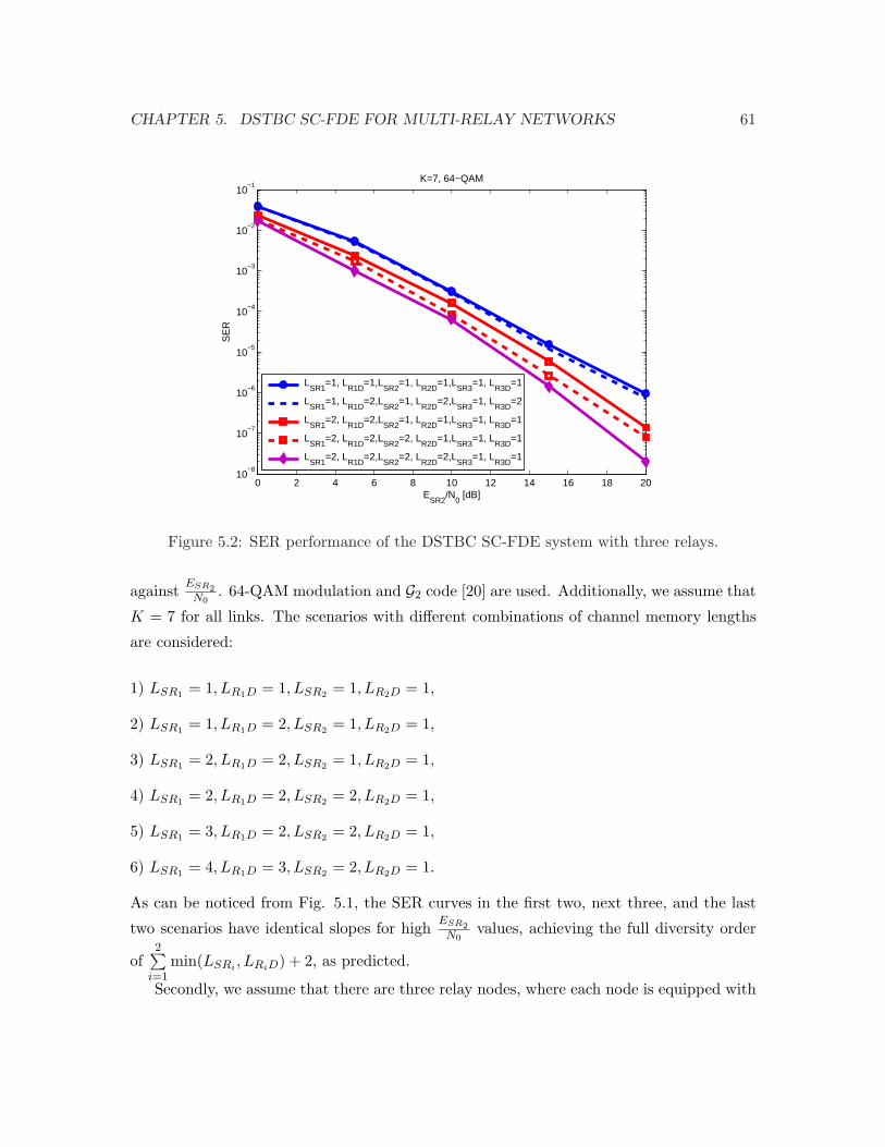
CHAPTER 5. DSTBC SC-FDE FOR MULTI-RELAY NETWORKS 61
0 2 4 6 8 10 12 14 16 18 2010
−8
10−7
10−6
10−5
10−4
10−3
10−2
10−1
ESR2
/N0 [dB]
SE
R
K=7, 64−QAM
LSR1
=1, LR1D
=1,LSR2
=1, LR2D
=1,LSR3
=1, LR3D
=1
LSR1
=1, LR1D
=2,LSR2
=1, LR2D
=2,LSR3
=1, LR3D
=2
LSR1
=2, LR1D
=2,LSR2
=1, LR2D
=1,LSR3
=1, LR3D
=1
LSR1
=2, LR1D
=2,LSR2
=2, LR2D
=1,LSR3
=1, LR3D
=1
LSR1
=2, LR1D
=2,LSR2
=2, LR2D
=2,LSR3
=1, LR3D
=1
Figure 5.2: SER performance of the DSTBC SC-FDE system with three relays.
against ESR2N0
. 64-QAM modulation and G2 code [20] are used. Additionally, we assume that
K = 7 for all links. The scenarios with different combinations of channel memory lengths
are considered:
1) LSR1 = 1, LR1D = 1, LSR2 = 1, LR2D = 1,
2) LSR1 = 1, LR1D = 2, LSR2 = 1, LR2D = 1,
3) LSR1 = 2, LR1D = 2, LSR2 = 1, LR2D = 1,
4) LSR1 = 2, LR1D = 2, LSR2 = 2, LR2D = 1,
5) LSR1 = 3, LR1D = 2, LSR2 = 2, LR2D = 1,
6) LSR1 = 4, LR1D = 3, LSR2 = 2, LR2D = 1.
As can be noticed from Fig. 5.1, the SER curves in the first two, next three, and the last
two scenarios have identical slopes for high ESR2N0
values, achieving the full diversity order
of2∑
i=1min(LSRi , LRiD) + 2, as predicted.
Secondly, we assume that there are three relay nodes, where each node is equipped with

CHAPTER 5. DSTBC SC-FDE FOR MULTI-RELAY NETWORKS 62
0 5 10 15 20 2510
−6
10−5
10−4
10−3
10−2
10−1
100
ESR2
/N0 [dB]
SE
R
LSR1
=1, LR1D
=2,LSR2
=1, LR2D
=2, 64−QAM
K=0K=25K=100
Figure 5.3: SER performance of the DSTBC SC-FDE system for different K-factor values.
one antenna. We set SNRSR1 = SNRSR3 = 25dB and ER1D = ER2D = ER3D = 5dB , and
the SER curve is plotted against ESR2N0
. 64-QAM modulation and G3 code [20] are used.
Additionally, we assume that K = 7 for all links. The scenarios with different combinations
of channel memory lengths are considered:
1) LSR1 = LR1D = LSR2 = LR2D = LSR3 = LR3D = 1,
2) LSR1 = LSR2 = LSR3 = 1, LR1D = LR2D = LR3D = 2,
3) LSR1 = LR1D = 2, LSR2 = LR2D = LSR3 = LR3D = 1,
4) LSR1 = LR1D = LSR2 = 2, LR2D = LSR3 = LR3D = 1,
5) LSR1 = LR1D = LSR2 = LR2D = 2, LSR3 = LR3D = 1,
As is illustrated in Fig. 5.2, first two and their next two scenarios have identical slopes for
high ESR2N0
values, achieving the full diversity order of3∑
i=1min(LSRi , LRiD) + 3, confirming
our conclusions from the PEP analysis.
Finally, the SER performance of the system is illustrated in Fig. 5.3 for different K-
factor values. We set SNRSR1 = 25dB and ER1D = ER2D = 5dB, and the SER curve is
plotted against ESR2N0
. 64-QAM modulation and G2 code [20] are used. Additionally, we
assume that LSR1 = LSR2 = 1 and LR1D = LR2D = 2 and plot the SER curves when
CHAPTER 5. DSTBC SC-FDE FOR MULTI-RELAY NETWORKS 63
K = 0, K = 25, and K = 100 for all of the underlying links. We remark that as the
K-factor of the Rician fading increases, the better SER performance is achieved, while the
diversity order remains unchanged.
As can be concluded from the simulation results that, in dual hop networks, the hop
with the smaller diversity order becomes the performance bottleneck.
5.6 Summary
In this chapter, by characterizing the channels as frequency-selective Rician fading, we have
derived theoretical PEP expression for distributed space-time block code in AF relaying
mode. Various numerical examples have been introduced to confirm our theoretical analysis.
Furthermore, we have investigated the performance of the distributed space-time block code
under different fading severity conditions.

Chapter 6
Conclusion
6.1 Conclusions
In this thesis, we investigate efficient equalization techniques for broadband wireless net-
works. These low-complexity and efficient equalization techniques address non-cooperative
and cooperative wireless networks.
We first study a new detection scheme for ZP-OFDM. We propose a novel reduced
complexity receiver design for ZP-OFDM transmissions, that not only outperforms MMSE-
ZP-OFDM, but also uses low-complexity computational methods that bring a significant
power saving to the proposed receiver. This makes it a strong candidate for WSNs which are
characterized by small and low-power devices. We show that linear processing collects both
multipath and spatial diversity gains, leading to significant improvement in performance,
while maintaining low complexity.
We next introduce a novel MMSE-based receiver design for SC-FDE. We propose a
novel reduced-complexity MMSE-based receiver design for D-STBC SC-FDE transmissions.
Specifically, we are considering AF relay networks for cooperative scenarios in which either
of S → R or R → D links are frequency selective Rician fading. We show that, by incorpo-
rating linear processing techniques, our MMSE-based receiver is able to collect full antenna
and multipath diversity gains, leading to significant improvement in performance at nearly
no additional complexity. Specifically, under the assumption of perfect power control and
high SNR for the underlying links and assuming either of S → R or R → D links to be
frequency selective Rician fading, our performance analysis demonstrates that the proposed
receiver is able to achieve a maximum diversity order of min(LSR, LRD) + LSD + 2, where
64

CHAPTER 6. CONCLUSION 65
LSR, LRD, and LSD are the channel memory lengths for S → R, R → D, and S → D links,
respectively. Complexity analysis and simulation results demonstrate that our proposed
receiver outperforms the conventional cooperative MMSE-SC-FDE receiver by performing
close to MFB, while providing minimal computational complexity.
Finally, we investigate the performance of D-STBC SC-FDE systems with AF relaying
over frequency-selective Rician fading channels in multi-relay networks. Our performance
analysis demonstrates that SC-FDE for DSTBC is able to achieve a maximum diversity
order ofR∑
i=1min(LSRi , LRiD) + R, where R is the number of participating relays, LSRi and
LRiD are the channel memory lengths for source to ith relay (S → Ri) link and ith relay to
destination (Ri → D) link , respectively.
6.2 Future works
The works in this thesis also reveal some interesting topics for future research. A particularly
intriguing problem is to analyze the efficiency of the low-complexity ZP-OFDM receiver
design described in chapter 3, as well as the efficient MMSE-based D-STBC SC-FDE receiver
described in chapter 4, in presence of multiple users.
In the study of DSTBC SC-FDE for multi-relay networks, we have mainly focused on
the application of different STBCs. This, however, brings about throughput loss and lower
efficiency. An interesting future work on this subject is to investigate a relay selective
algorithm for frequency selective channels that makes up for the STBC rate loss.

Bibliography
[1] B. Muquet, Z. Wang, G. B. Giannakis, M. de Courville, and P. Duhamel, “Cyclic pre-fixing or zero padding for wireless multicarrier transmissions?” IEEE Trans. Commun,vol. 50, pp. 2136–2148, 2002.
[2] H. Eghbali, S. Muhaidat, and N. Al-Dhahir, “A novel reduced complexity mmse-basedreceiver for ofdm broadband wireless networks,” in IEEE Wireless Comm. and Net-working Conf. (WCNC), Sydney, Aus, 2010.
[3] H. Mheidat, M. Uysal, and N. Al-Dhahir, “Equalization techniques for distributedspace-time block codes with amplify-and-forward relaying,” IEEE Trans. on SignalProc, vol. 55, no. 5, 2007.
[4] D. Y. Seol, U. K. Kwon, and E. S. Kim, “Relay-assisted sfbc single carrier transmissionover uplink fast fading channels,” in Proc. IEEE GLOBECOM, 2007.
[5] H. Eghbali, S. Muhaidat, and N. Al-Dhahir, “A low complexity two stage mmse-basedreceiver for single-carrier frequency-domain equalization transmissions over frequency-selective channels,” in Proc. IEEE GLOBECOM, Honolulu, Hawaii, USA, 2009.
[6] S. Y. Hui and K. H. Yeung, “Challenges in the migration to 4g mobile systems,” IEEECommun. Mag., vol. 41, pp. 54 – 59, 2003.
[7] T. S. Rappaport, Wireless Communications: Principles and Practice, 2nd ed. UpperSaddle River, NJ: Prentice-Hall, 2002.
[8] W. C. Jakes, Microwave Mobile Communications, 1st ed. New York: John Wiley andSons, 1974.
[9] D. Tse and P. Viswanath, Fundamentals of Wireless Communication. CambridgeUniversity Press, 2005.
[10] S. M. Alamouti, “A simple transmit diversity technique for wireless communications,”IEEE J. Sel. Areas Commun., vol. 16, pp. 1451–1458, 1998.
[11] J. Rogers and C. Plett, Radio frequency integrated circuit design, 2nd ed. London,United Kingdom: Artech House, 2010.
66
BIBLIOGRAPHY 67
[12] A. Wittneben, “Base station modulation diversity for digital simulcast,” in Proc. ofVehicular Technology Conference. VTC-93., 1993, pp. 505–511.
[13] ——, “A new bandwidth efficient transmit antenna modulation diversity scheme forlinear digital modulation,” in Proceedings of the IEEE International Conference Com-munications (ICC), 1993, pp. 1630–1634.
[14] J. H. Winters, “Diversity gain of transmit diversity in wireless systems with rayleighfading,” IEEE Trans. Veh. Technol., vol. 47, pp. 119–123, 1998.
[15] V. Tarokh, N. Seshadri, and A. R. Calderbank, “Space-time codes for high data ratewireless communication: Performance criterion and code construction,” IEEE Trans.Inf. Theory, vol. 44, pp. 744–765, 1998.
[16] J. G. Foschini, “Layered space-time architecture for wireless communication in a fadingenvironment when using multi element antennas,” Bell Labs Tech. J., vol. 2, pp. 41–59,1996.
[17] C. Kose and R. D. Wesel, “Universal space-time trellis codes,” IEEE Trans. Inf. Theory,vol. 49, pp. 2717–2727, 2003.
[18] Z. Safar and K. J. R. Liu, “Systematic space-time trellis code construction for corre-lated rayleigh-fading channels,” IEEE Trans. Inf. Theory, vol. 50, pp. 2855–2865, 2004.
[19] L. Yonghui, B. Vucetic, Y. Tang, and Q. Zhang, “Space-time trellis codes with li-neartransformation for fast fading channels,” IEEE Signal Process. Lett., vol. 50, no. 11,pp. 895– 898, 2004.
[20] V. Tarokh, H. Jafarkhani, and A. R. Calderbank, “Space-time block codes from or-thogonal designs,” IEEE Trans. Inf. Theory, vol. 45, pp. 1456–1467, 1999.
[21] V. Tarokh, A. Naguib, N. Seshadri, and A. R. Calderbank, “Spacetime codes for wire-less communication: Combined array processing and space time coding,” IEEE Trans.Inf. Theory, vol. 45, 1998.
[22] H. Wang and X.-G. Xia, “Upper bounds of rates of complex orthogonal space-timeblock codes,” IEEE Trans. Inf. Theory, vol. 49, no. 10, pp. 2788–2796, 2003.
[23] S. Das, N. Al-Dhahir, and R. Calderbank, “Novel full-diversity high-rate stbc for 2 and4 transmit antennas,” IEEE Commun. Lett., vol. 10, no. 3, pp. 171–173, 2006.
[24] H. Jafarkhani and N. Seshadri, “Super-orthogonal space-time trellis codes,” IEEETrans. Inf. Theory, vol. 49, no. 4, pp. 937–950, 2003.
[25] B. Hassibi and B. Hochwald, “High-rate codes that are linear in space and time,” IEEETrans. Inf. Theory, vol. 48, no. 7, pp. 1804–1824, 2002.
BIBLIOGRAPHY 68
[26] R. W. Heath and A. Paulraj, “Linear dispersion codes for mimo systems based onframe theory,” IEEE Trans. Signal Process., vol. 50, no. 10, pp. 2429–2441, 2002.
[27] B. Vucetic and J. Yuan, Space-Time Coding. John Wiley & Sons, 2003.
[28] A. Paulraj, D. Gore, and R. Nabar, Introduction to Space-Time Wireless Communica-tions. Cambridge University Press, 2003.
[29] H. Jafarkhani, Space-Time Coding: Theory and Practice. Cambridge University Press,2005.
[30] A. Sendonaris, E. Erkip, and B. Aazhang, “User cooperation diversity part i: systemdescription,” IEEE Trans. Comm., vol. 51, no. 11, 2003.
[31] ——, “User cooperation diversity part ii: implementation aspects and performanceanalysis,” IEEE Trans. Comm., vol. 51, no. 11, 2003.
[32] J. N. Laneman, G. W. Wornell, and D. N. C. Tse, “An efficient protocol for realizingcooperative diversity in wireless networks,” Washington, DC.
[33] J. N. Laneman, D. N. C. Tse, and G. W. Wornell, “Cooperative diversity in wirelessnetworks: Efficient protocols and outage behavior,” IEEE Trans. Inf. Theory, 2004.
[34] J. N. Laneman and G. W. Wornell, “Distributed space-time-coded protocols for ex-ploiting cooperative diversity in wireless networks,” IEEE Trans. Inf. Theory, vol. 49,no. 10, 2003.
[35] E. V. D. Meulen, “Advances in applied probability,” Advances in Applied Probability,vol. 3, pp. 120–154, 1971.
[36] T. M. Cover and A. E. Gamal, “Capacity theorems for the relay channel,” IEEE Trans.Inf. Theory, vol. 25, no. 5, 1979.
[37] T. E. Hunter and A. Nosratinia, “Cooperative diversity through coding,” in Proc. IEEEISIT, Lausanne, Switzerland, 2002.
[38] ——, “Diversity through coded cooperation,” IEEE Trans. Wireless Commun., vol. 5,no. 2, pp. 283–289, 2006.
[39] R. U. Nabar, H. Bolcskei, and F. Kneubuhler, “Fading relay channels: Performancelimits and space-time signal design,” IEEE J. Sel. Areas Comm., vol. 22, no. 6.
[40] A. Azarian, H. EL Gamal, and P. Schniter, “On the achievable diversity multiplexingtradeoff in half-duplex cooperative channels,” IEEE Trans. Inf. Theory, vol. 51, pp.4152–4172, 2005.
[41] J. E. Padgett, C. G. Gunther, and T. Hattori, “Overview of wireless personal commu-nications,” IEEE Commun. Mag., vol. 33, no. 1, pp. 28–41, 1995.
BIBLIOGRAPHY 69
[42] J. D. Parsons, The Mobile Radio Propagation Channel, 2nd ed. Singapore: JohnWiley & Sons, 2000.
[43] A. Goldsmith, Wireless Communications, 1st ed. UK: Cambridge University Press,2005.
[44] D. Falconer and et. al., “Frequency domain equalization for single-carrier broadbandwireless systems,” IEEE Commun. Mag., vol. 40, no. 4, pp. 58–66, 2002.
[45] H. Sari, G. Karam, and I. Jeanclaude, “Frequency-domain equalization of mobile radioand terrestrial broadcast channels,” in Proc. of Global Telecommunications Conference.GLOBECOM-94, 1994, p. 15.
[46] Z. Wang and G. B. Giannakis, “Linearly precoded or coded ofdm against wirelesschannel fades?” in Proc. of the IEEE Workshop on Signal Processing Advances forWireless Communications, Taiwan, China, 2001.
[47] W. W. Lu, “Compact multidimensional broadband wireless: The convergence of wire-less mobile and access,” IEEE Commun. Mag., pp. 119–23, 2000.
[48] S. Govardhanagiri, T. Karp, P. Heller, and T. Nguyen, “Performance analysis of mul-ticarrier modulations systems using cosine modulated filterbanks,” in Proc. ICASSP.
[49] D. P. Palomar, J. M. Cioffi, and M. A. Lagunas, “Joint tx-rx beamforming designfor multicarrier mimo channels: a unified framework for convex optimization,” IEEETrans. Signal Process, vol. 51, no. 9, 2003.
[50] W. Zou and Y. Wu, “Cofdm : an overview,” IEEE Trans. Broadcast, vol. 41, 1995.
[51] D. Divsalar and M. K. Simon, “Multiple trellis coded modulation (mtcm),” IEEETrans. Commun, vol. 36, 1988.
[52] ——, “Error bounds for convolutional codes and an asymptotically optimum decodingalgorithm,” IEEE Trans. Inform. Theory, vol. IT-13, 1967.
[53] L. Lee, “Space-time bit-interleaved coded modulation for ofdm systems,” IEEE Trans.Signal Process, vol. 52, 2004.
[54] Z. Liu, Y. Xin, and G. B. Giannakis, “Linear constellation precoding for ofdm withmaximum multipath diversity and coding gains,” IEEE Trans. Commun, vol. 51, 2003.
[55] J. Boutros and E. Viterbo, “Signal space diversity: a power- and bandwidth-efficientdiversity technique for the rayleigh fading channel,” IEEE Trans. Inform. Theory,vol. 44, 1998.
[56] A. O. Hero and T. L. Marzetta, “Cutoff rate and signal design for the quasi-staticrayleigh fading space-time channel,” IEEE Trans. Inform. Theory, vol. 47, 2001.

BIBLIOGRAPHY 70
[57] Y. Rong, S. A. Vorobyov, and A. B. Gershman, “Linear block precoding for ofdmsys-tems based on maximization of mean cutoff rate,” IEEE Trans. Signal Process, vol. 53,no. 12, 2005.
[58] O. Edfors, M. Sandell, J. J. van de Beek, and P. O. Brjesson, “Ofdm channel estimationby singular value decomposition,” IEEE Comm. Lett., vol. 46, no. 7, pp. 931–939, 1998.
[59] J. Coon, S. Armour, M. Beach, and J. McGeehan, “Adaptive frequency-domain equal-ization for single-carrier multiple-input multiple-output wireless transmissions,” IEEETrans. on Signal Proc, vol. 53, no. 8, pp. 3247–3256, 2005.
[60] A. Scaglione, G. B. Giannakis, and S. Barbarossa, “Redundant filterbank precodersand equalizers - part i : Unification and optimal designs and part ii : Blind chan-nel estimation, synchronization and direct equalization,” IEEE Trans. Signal Process,vol. 47, 1999.
[61] M. K. Simon and M. S. Alouini, Digital Communication Over Fading Channels: AUnified Approach to Performance Analysis. New York: Wiley-Intersci., 2000.
[62] A. Stuart and J. K. Ord, Kendall’s Advanced Theory of Statistics, 5th ed. London,U.K.: Griffin, 1987.
[63] J. Lu, T. T. Tjhung, F. Adachi, and C. L. Huang, “Ber performance of ofdm-mdpsksystem in frequency-selective rician fading with diversity reception,” IEEE Trans. onVeh. Technol., vol. 49, no. 4, pp. 1216–1225, 2000.
[64] N. Al-Dhahir, “Single-carrier frequency-domain equalization for spacetime block-codedtransmissions over frequency-selective fading channels,” Electron. Lett., vol. 5, pp. 304–306, 2001.
[65] M. Uysal, O. Campolat, and M. M. Fareed, “Asymptotic performance analysis of dis-tributed space-time codes,” IEEE Commun. Lett., vol. 10, no. 11, pp. 775–777, 2006.
[66] O. Canpolat, M. Uysal, and M. M. Fareed, “Analysis and design of distributed space-time trellis codes with amplify-and-forward relaying,” IEEE Trans. Veh. Technol.,vol. 56, pp. 1649–1660, 2007.
[67] R. U. Nabar1 and H. Bolcskei, “Space-time signal design for fading relay channels,” inProc. IEEE GLOBECOM, vol. 4, San Francisco, CA., 2003.