SILC QRINT A PL 2008 0000 V0001 N - circabc.europa.eu... central statistical office of poland...

CENTRAL STATISTICAL OFFICE OF POLAND

INTERIM REPORT

GRANT AGREEMENT

NO 36401.2007.001-2007.161

ACTION ENTITLED:

EU-SILC 2008

Warsaw, November 2009

"This document has been produced with the financial assistance of the European Community. The views expressed herein are those of the author and can therefore in no way be taken to reflect the official opinion of the European Commission."

2

CONTENTS Page PREFACE 3 1. COMMON CROSS-SECTIONAL EUROPEAN UNION INDICATO RS.................. 4

1.1. Common cross-sectional EU indicators based on the cross-sectional component of EU-SILC ................................................................................................................... 4

2. ACCURACY...................................................................................................................... 5

2.1. Sample design ................................................................................................................. 5 2.1.1. Type of sampling design.................................................................................................. 5 2.1.2. Sampling units ................................................................................................................. 5 2.1.3. Stratification and substratification criteria..................................................................... 5 2.1.4. Sample size and allocation criteria................................................................................. 5 2.1.5. Sample selection schemes................................................................................................ 6 2.1.7. Renewal of sample: rotational groups ............................................................................ 6 2.1.8. Weightings....................................................................................................................... 6 2.1.9. Substitutions .................................................................................................................... 9

2.2. Sampling errors ............................................................................................................... 9 2.2.1. Standard error and effective sample size ........................................................................ 9

2.3. Non-sampling errors...................................................................................................... 12 2.3.1. Sampling frame and coverage errors............................................................................ 12 2.3.2. Measurement and processing errors............................................................................. 12 2.3.3. Non-response errors...................................................................................................... 14

2.4. Mode of data collection................................................................................................. 22

2.5. Interview duration ......................................................................................................... 23 3. COMPARABILITY........................................................................................................ 24

3.1. Basic concepts and definitions ...................................................................................... 24

3.2. Components of income.................................................................................................. 26 3.2.1. Differences between the national definitions and standards EU-SILC definitions,

and an assessment ......................................................................................................... 26 3.2.2. The source or procedure used for the collection of income variables .......................... 28 3.2.3. The form in which income variables at component level have been obtained.............. 28 3.2.4. The method used for obtaining income target variables in the required form ............ 28 4. COHERENCE ................................................................................................................. 29

4.1. Comparison of EU-SILC and HBS results....................................................................... 29

4.2. Comparison of Laeken Indicators based on EU-SILC 2007 and EU-SILC 2008............ 32

4.3. Comparison of 2007 results of SNA and EU-SILC 2008 (data for 2007) for Poland......................................................................................................................... 32

3

PREFACE The present quality report is the intermediate quality report of EU-SILC 2008 in Poland

according to grant agreement No. 36401.2007.001-2007.161 and follows the structure

outlined in the Commission Regulation No. 1177/2003.

This report consists of four chapters.

The first chapter describes the common cross-sectional indicators and other indicators

of interest computed on the basis of EU-SILC 2008.

The second chapter deals with accuracy i.e. here should be described all the factors that affect

the precision of estimations and results.

The third chapter reports on comparability and indicates all differences between the standard

EU definitions and those applied in the polish survey.

The fourth and last chapter, reporting on coherence, presents the comparisons of the EU-SILC

2008 data with external sources.

As this is the fourth intermediate quality report for EU-SILC in Poland some chapters and

sections resemble the corresponding chapters and sections of the preceding reports.

4

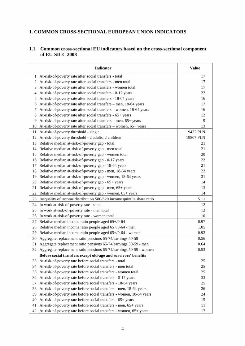
1. COMMON CROSS-SECTIONAL EUROPEAN UNION INDICATORS 1.1. Common cross-sectional EU indicators based on the cross-sectional component

of EU-SILC 2008

Indicator Value

1 At-risk-of-poverty rate after social transfers - total 17 2 At-risk-of-poverty rate after social transfers - men total 17 3 At-risk-of-poverty rate after social transfers - women total 17 4 At-risk-of-poverty rate after social transfers - 0-17 years 22 5 At-risk-of-poverty rate after social transfers - 18-64 years 16 6 At-risk-of-poverty rate after social transfers – men, 18-64 years 17 7 At-risk-of-poverty rate after social transfers – women, 18-64 years 16 8 At-risk-of-poverty rate after social transfers - 65+ years 12 9 At-risk-of-poverty rate after social transfers – men, 65+ years 9

10 At-risk-of-poverty rate after social transfers – women, 65+ years 13

11 At-risk-of-poverty threshold - single 9432 PLN 12 At-risk-of-poverty threshold - 2 adults, 2 children 19807 PLN

13 Relative median at-risk-of-poverty gap - total 21 14 Relative median at-risk-of-poverty gap - men total 21 15 Relative median at-risk-of-poverty gap - women total 20 16 Relative median at-risk-of-poverty gap - 0-17 years 22 17 Relative median at-risk-of-poverty gap - 18-64 years 21 18 Relative median at-risk-of-poverty gap - men, 18-64 years 22 19 Relative median at-risk-of-poverty gap - women, 18-64 years 21 20 Relative median at-risk-of-poverty gap - 65+ years 14 21 Relative median at-risk-of-poverty gap - men, 65+ years 13 22 Relative median at-risk-of-poverty gap - women, 65+ years 14

23 Inequality of income distribution S80/S20 income quintile share ratio 5.11

24 In work at-risk-of-poverty rate - total 12 25 In work at-risk-of-poverty rate - men total 12 26 In work at-risk-of-poverty rate - women total 10

27 Relative median income ratio people aged 65+/0-64 0.97 28 Relative median income ratio people aged 65+/0-64 - men 1.05 29 Relative median income ratio people aged 65+/0-64 - women 0.92

30 Aggregate replacement ratio pensions 65-74/earnings 50-59 0.56 31 Aggregate replacement ratio pensions 65-74/earnings 50-59 - men 0.64 32 Aggregate replacement ratio pensions 65-74/earnings 50-59 - women 0.53

Before social transfers except old-age and survivors' benefits 33 At-risk-of-poverty rate before social transfers - total 25 34 At-risk-of-poverty rate before social transfers - men total 25 35 At-risk-of-poverty rate before social transfers - women total 25 36 At-risk-of-poverty rate before social transfers - 0-17 years 33 37 At-risk-of-poverty rate before social transfers - 18-64 years 25 38 At-risk-of-poverty rate before social transfers - men, 18-64 years 26 39 At-risk-of-poverty rate before social transfers - women, 18-64 years 24 40 At-risk-of-poverty rate before social transfers - 65+ years 15 41 At-risk-of-poverty rate before social transfers - men, 65+ years 11 42 At-risk-of-poverty rate before social transfers - women, 65+ years 17

5

Indicator Value

Before social transfers including old-age and survivors' benefits

43 At-risk-of-poverty rate before social transfers - total 44

44 At-risk-of-poverty rate before social transfers - men total 42

45 At-risk-of-poverty rate before social transfers - women total 46

46 At-risk-of-poverty rate before social transfers - 0-17 years 38

47 At-risk-of-poverty rate before social transfers - 18-64 years 38

48 At-risk-of-poverty rate before social transfers - men, 18-64 years 37

49 At-risk-of-poverty rate before social transfers - women, 18-64 years 39

50 At-risk-of-poverty rate before social transfers - 65+ years 85

51 At-risk-of-poverty rate before social transfers - men, 65+ years 85

52 At-risk-of-poverty rate before social transfers - women, 65+ years 85

53 Mean equivalised disposable income 18684 PLN

2. ACCURACY 2.1. Sample design 2.1.1. Type of sampling design The two-stage sampling scheme with differentiated selection probabilities at the first stage was used. Prior to selection, sampling units were stratified. 2.1.2. Sampling units The first-stage sampling units (primary sampling units - PSU) were enumeration census areas, while at the second stage dwellings were selected. All the households from the selected dwellings are supposed to enter the survey. 2.1.3. Stratification and substratification criteria The strata were the voivodships (NUTS2) and within voivodships primary sampling units were classified by class of locality. In urban areas census areas were grouped by size of town, but in the five largest cities districts were treated as strata. In rural areas strata were represented by rural gminas (NUTS5) of a subregion (NUTS3) or of a few neighbouring poviats (NUTS4). Altogether 211 strata were distinguished. 2.1.4. Sample size and allocation criteria It was decided that the sample should include about 24 000 dwellings in the first year of the survey. Proportional allocation of dwellings to particular strata was applied. The number of dwellings selected from a particular stratum was in proportion to the number of dwellings in the stratum. Furthermore, the number of the first-stage units selected from the strata was obtained by dividing the number of dwellings in the sample by the number of dwellings determined for a given class of locality to be selected from the first-stage unit. In towns with

6

over 100 000 population 3 dwellings per PSU were selected, in towns with 20-100 thousand population – 4 dwellings per PSU, in towns with less than 20 000 population – 5 dwellings per PSU, respectively. In rural areas 6 dwellings were selected from each PSU. Altogether 5912 census areas and 24044 dwellings were selected for the sample in the first year of the survey. The subsample 5 selected for the survey in 2006 to replace the subsample 1 consisted of 1476 census areas and 6002 dwellings. Then, in 2007 the subsample 6 replaced the subsample 2 and consisted of 1478 census areas and 6008 dwellings. For the 2008 survey the subsample 3 was replaced by the subsample 7. This new subsample consisted of 1479 census areas and 6016 dwellings. 2.1.5. Sample selection schemes Census areas were selected according to the Hartley-Rao scheme. Prior to selection, census areas were put in random order for each stratum separately and then the determined number of PSU was selected with probabilities proportionate to the number of dwellings. Then in each of the census areas belonging to the PSU sample dwellings were selected using the simple random selection procedure. 2.1.7. Renewal of sample: rotational groups The selected sample of first-stage units was divided into four subsamples, equal in size. Starting from 2006 one of the subsamples is eliminated and replaced with a new one, selected independently as described above. For the 2006 survey the subsample 5 was selected as a replacement of the subsample 1. Then, for the 2007 survey the subsample 6 was selected which replaced the subsample 2. For the 2008 survey the new subsample 7 replaced subsample 3. 2.1.8. Weightings Design factor Design factor – DB080 is equal to the dwelling sampling fraction reciprocal in the h-th stratum i.e.

,M

mnfh

hhh

′∗=

fDB

h

1080 =

where: nh - number of PSU selected from the h-th stratum, m’h - number of dwellings selected from a PSU in the h-th stratum, Mh – number of dwellings in the h-th stratum.

7

Non-response adjustments DB080 weights were then adjusted with the use of household non-response rates estimated for each class of locality separately:

Code of class of locality

(p)

Class of locality Completeness rate

(crp=Rap*Rh p)

Poland 0.654

1 Warsaw 0.404

2 Towns 500 000 – 1 000 000 inhabitants 0.535

3 Towns 100 000 – 500 000 inhabitants 0.581

4 Towns 20 000 – 100 000 inhabitants 0.637

5 Towns less than 20 000 inhabitants 0.665

6 Rural areas 0.787

The adjusted weights were calculated according to the formula:

,080

080RhRa

DBDB

pp

pcorrectedp ∗

=

Weights DB080 and DB080corrected were calculated for the subsample 7. The next step consisted in calculating the weights DB090 for the households and RB050 for all household members of the subsample 7 with the use of the integrated calibration method. For the subsamples 5 surveyed for the third time and 6 surveyed for the second time and the subsample 4 surveyed for the four time the base weights were determined by the correction of the base weights from the previous year. For the subsample 6 the following method was used: The base weight of 2007 is equal to RB050 multiplied by 4. This weight was then adjusted by non-response and households’ and individuals’ falling out of the population surveyed. The calculations were made on the subsamples of the so called sample persons i.e. those who were in the surveyed sample at the age of 14 and over in 2007 and who should be surveyed in 2008. The modifying factor was determined according to the class of locality and took the form:

( )( )2

1

RMR

p

p−

where: R(t)p – estimated number of respondents belonging to the sample person group in the p-th

class of locality in the subsample surveyed for the t-th time, M – estimated number of sample persons who belonged to the surveyed population in the first

year and in the next year were out of the survey scope.

8

The base weights of 2007 were used for the calculation of numerator and denominator. The above expression is the reciprocal of the empirical estimate of probability that a given person will be interviewed again in the second year of the survey. In the second stage of the base weight calculation for the second year of the survey children of “sample persons” received the weights of mothers and “co-residents’ i.e. additional persons included in the household surveyed were ascribed zero weights. Then the respondents’ base weights were averaged and all the members of a given household were ascribed such a mean weight. Then for the weights thus obtained the trimming of extreme weights was applied. For the subsamples 4 and 5 (surveyed for the fourth and third time respectively) algorithm based on method described for the subsample 6 was used. Additionally, re-entries occurrence was taken into account i.e. persons who were surveyed in 2006, not surveyed in 2007, and again surveyed in 2008 year. The base weights for such persons were computed by correction of base weights from year 2006 on data for years 2006 and 2008 (without information from 2007 year). Inclusion of re-entries to the subsamples surveyed in 2008 year caused the necessity of additional correction of the base weights for persons surveyed in the three successive years. Coefficients of these corrections were computed separately according to classes of locality as ratios: weighted number of respondents surveyed in all three years to the weighted number of respondents in the last survey year (i.e. with re-entries); weight used in these calculations was the weight RB050 for year 2006. Computed coefficients are shown in the following table:

Class of locality Correction for subsample 4

Correction for subsample 5

1 0.938 1.000

2 0.976 0.953

3 0.990 0.992

4 0.990 0.987

5 0.994 0.986

6 0.994 0.989

The last stage of the base weight calculation for the fourth year of the survey consisted in receiving weights of mothers by children of “sample persons” and zero weights by “coresidents’ i.e. additional persons included in the households. Then the respondents’ base weights were averaged and all the members of a given household were ascribed such a mean weight. Then for the weights thus obtained the trimming of extreme weights was applied. The last stage of calculations consisted in combining the four independent subsamples, applying the integrated calibration as described below (for the sample 7 repeatedly) and trimming. As a result, DB090 and RB050 weights are obtained for households and individuals from the samples 4, 5, 6 and 7.

9

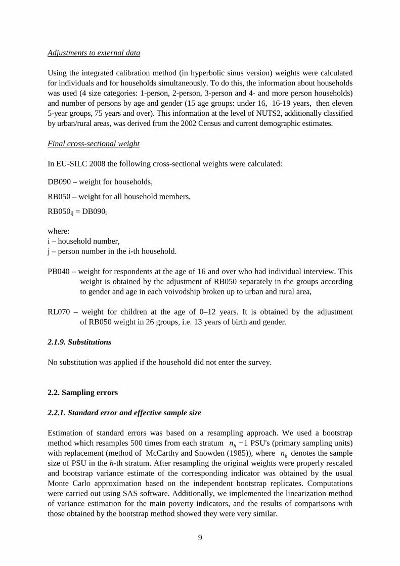
Adjustments to external data Using the integrated calibration method (in hyperbolic sinus version) weights were calculated for individuals and for households simultaneously. To do this, the information about households was used (4 size categories: 1-person, 2-person, 3-person and 4- and more person households) and number of persons by age and gender (15 age groups: under 16, 16-19 years, then eleven 5-year groups, 75 years and over). This information at the level of NUTS2, additionally classified by urban/rural areas, was derived from the 2002 Census and current demographic estimates. Final cross-sectional weight In EU-SILC 2008 the following cross-sectional weights were calculated: DB090 – weight for households, RB050 – weight for all household members, RB050ij = DB090i

where: i – household number, j – person number in the i-th household. PB040 – weight for respondents at the age of 16 and over who had individual interview. This

weight is obtained by the adjustment of RB050 separately in the groups according to gender and age in each voivodship broken up to urban and rural area,

RL070 – weight for children at the age of 0–12 years. It is obtained by the adjustment

of RB050 weight in 26 groups, i.e. 13 years of birth and gender. 2.1.9. Substitutions No substitution was applied if the household did not enter the survey. 2.2. Sampling errors 2.2.1. Standard error and effective sample size Estimation of standard errors was based on a resampling approach. We used a bootstrap method which resamples 500 times from each stratum 1−hn PSU's (primary sampling units) with replacement (method of McCarthy and Snowden (1985)), where hn denotes the sample size of PSU in the h-th stratum. After resampling the original weights were properly rescaled and bootstrap variance estimate of the corresponding indicator was obtained by the usual Monte Carlo approximation based on the independent bootstrap replicates. Computations were carried out using SAS software. Additionally, we implemented the linearization method of variance estimation for the main poverty indicators, and the results of comparisons with those obtained by the bootstrap method showed they were very similar.

10

Indicator Value Standard

error

Achieved sample

size

Design effect

Effective sample

size

At-risk-of-poverty rate after social transfers - total 16.88 0.42 41200 4.19 9829

At-risk-of-poverty rate after social transfers - men total 17.03 0.46 19772 2.42 8172

At-risk-of-poverty rate after social transfers - women total 16.74 0.44 21428 2.41 8909

At-risk-of-poverty rate after social transfers - 0-17 years 22.44 0.74 8743 2.12 4127

At-risk-of-poverty rate after social transfers - 18-64 years 16.27 0.43 26462 2.85 9296

At-risk-of-poverty rate after social transfers - men 18-64 years 16.77 0.47 12923 1.68 7704

At-risk-of-poverty rate after social transfers - women 18-64 years 15.79 0.45 13539 1.64 8263

At-risk-of-poverty rate after social transfers - 65+ years 11.72 0.53 5995 1.15 5209

At-risk-of-poverty rate after social transfers - men 65+ years 8.87 0.75 2378 1.02 2338

At-risk-of-poverty rate after social transfers - women 65+ years 13.42 0.64 3617 0.99 3643

At-risk-of-poverty threshold - single 9432 70 41200 3.56 11587

At-risk-of-poverty threshold - 2 adults, 2 children 19807 146 41200 3.56 11587

Relative median at-risk-of-poverty gap - total 20.55 0.72 41200 5.59 7371

Relative median at-risk-of-poverty gap - men total 21.45 0.82 19772 2.14 9247

Relative median at-risk-of-poverty gap - women total 19.96 0.70 21428 2.23 9604

Relative median at-risk-of-poverty gap - 0-17 years 21.92 1.24 8743 2.53 3451

Relative median at-risk-of-poverty gap - 18-64 years 21.47 0.82 26462 2.53 10470

Relative median at-risk-of-poverty gap - men, 18-64 years 22.11 0.85 12923 1.61 8007

Relative median at-risk-of-poverty gap - women, 18-64 years 20.69 0.90 13539 1.70 7960

Relative median at-risk-of-poverty gap - 65+ years 13.77 0.88 5995 1.02 5860

Relative median at-risk-of-poverty gap - men, 65+ years 12.81 1.62 2378 0.90 2644

Relative median at-risk-of-poverty gap - women, 65+ years 13.84 1.01 3617 1.07 3388

Inequality of income distribution S80/S20 income quintile share ratio 5.11 0.10 41200 3.31 12445

In work at-risk-of-poverty rate - total 11.51 0.42 14558 1.93 7536

In work at-risk-of-poverty rate - men total 12.41 0.48 7914 1.31 6044

In work at-risk-of-poverty rate - women total 10.36 0.46 6644 1.23 5421

Relative median income ratio people aged 65+/0-64 0.97 0.01 41200 1.32 31119

Relative median income ratio people aged 65+/0-64 - men 1.05 0.02 19772 0.89 22315

Relative median income ratio people aged 65+/0-64 - women 0.92 0.01 21428 1.41 15177

Aggregate replacement ratio pensions 65-74/earnings 50-59 0.56 0.01 5593 1.08 5185

Aggregate replacement ratio pensions 65-74/earnings 50-59 - men 0.64 0.02 2842 1.00 2839

Aggregate replacement ratio pensions 65-74/earnings 50-59 - 0.53 0.02 2751 1.03 2660

11


error

Achieved sample

size

Design effect

Effective sample

size

women

Before social transfers except old-age and survivors' benefits

At-risk-of-poverty rate before social transfers - total 25.06 0.48 41200 3.92 10511

At-risk-of-poverty rate before social transfers - men total 25.36 0.52 19772 2.08 9493

At-risk-of-poverty rate before social transfers - women total 24.78 0.50 21428 2.32 9256

At-risk-of-poverty rate before social transfers - 0-17 years 32.51 0.81 8743 2.08 4211


At-risk-of-poverty rate before social transfers - men, 18-64 years 25.61 0.56 12923 1.59 8127

At-risk-of-poverty rate before social transfers - women, 18-64 years 24.26 0.55 13539 1.79 7577

At-risk-of-poverty rate before social transfers - 65+ years 14.76 0.58 5995 1.22 4906

At-risk-of-poverty rate before social transfers - men, 65+ years 11.18 0.84 2378 1.09 2187

At-risk-of-poverty rate before social transfers - women, 65+ years 16.91 0.69 3617 0.96 3765


At-risk-of-poverty rate before social transfers - total 44.09 0.57 41200 3.60 11452

At-risk-of-poverty rate before social transfers - men total 41.84 0.62 19772 2.17 9118

At-risk-of-poverty rate before social transfers - women total 46.19 0.58 21428 2.07 10349



At-risk-of-poverty rate before social transfers - men, 18-64 years 36.65 0.64 12923 1.59 8126

At-risk-of-poverty rate before social transfers - women, 18-64 years 38.55 0.60 13539 1.64 8247

At-risk-of-poverty rate before social transfers - 65+ years 84.93 0.60 5995 1.41 4249

At-risk-of-poverty rate before social transfers - men, 65+ years 84.91 0.95 2378 1.05 2269

At-risk-of-poverty rate before social transfers - women, 65+ years 84.94 0.64 3617 0.98 3690

Mean equivalised disposable income 18684.46 162.16 41200 3.57 11539

12


error

Achieved sample

size

Design effect

Effective sample

size

Gini coefficient 32.01 0.42 41200 3.15 13072

2.3. Non-sampling errors 2.3.1. Sampling frame and coverage errors

The samples for EU-SILC were selected from the sampling frame based on the TERYT system, i.e. the Domestic Territorial Division Register. Two kinds of primary sampling units (PSU) were distinguished in the sampling frame:

- about 178 000 CEA – census enumeration areas with about 68 dwellings each, - about 33 000 ESD – enumeration statistical districts, with about 377 dwellings each.

The whole territory of Poland is divided into enumeration statistical districts and census enumeration areas. In EU-SILC census enumeration areas are used as primary sampling units. The secondary sampling units are dwellings. For each census enumeration area a list of dwellings was made up to form the secondary sampling frame. All the households from the selected dwellings are supposed to enter the survey. The TERYT system is updated annually with respect to the territorial division into statistical districts and census enumeration areas. The lists of dwellings, names of towns, villages and streets are updated. Other changes due to new construction, dismantle of buildings and administrative division modifications are also introduced. The sample for EU-SILC 2005 was selected in September 2004 from the sampling frame updated as for January 1, 2004. In the sample selected some 6.8% of dwellings were found to be non-existing (cancelled, changed for non-residential units) as well as uninhabited or temporarily inhabited, while in the sample 5 selected in 2005 for the 2006 survey about 6.2% of such dwellings were recorded. In the sample 6 selected for the 2007 survey there were about 7% of such dwellings, and in the sample 7 selected for the 2008 survey there were about 6.3% of such dwellings. 2.3.2. Measurement and processing errors As with any other statistical survey, EU-SILC may be burdened with non-sampling errors which occur at various stages of the survey and which cannot be eliminated completely. This mainly applies to interviewers’ errors at the stage of collecting the information, errors due to the respondents’ misunderstanding of questions and inaccurate or sometimes even false answers as well as the errors taking place at the stage of data recording. After the household and individual interview completion the respondents were obliged to answer a few questions concerning interview performance. On the basis of this material it is possible to state that about three quarters of respondents (80% of those filling in the household questionnaire and 78% of those filling in the individual questionnaire) showed a favourable attitude towards the survey, while about 3% (both in the case of the household

13

and individual interview) were unwilling towards it. In the interviewers’ opinion, in about 89% of questionnaires (both household and individual ones) the quality of non-income data collected could be recognised as good or very good and in 1% - as doubtful. The quality of income data was evaluated as slightly worse, mainly because of item non-response. It should also be pointed out that, in our opinion, the quality of data concerning net income categories is much higher than in the case of gross income. The reason is that non-response to the highest degree affected the information on taxes and social and health insurance contributions. In Poland, the EU-SILC survey in 2008 was carried out in May/June. EU-SILC, as it was in 2005, 2006 and 2007, is a non-obligatory, representative survey of individual households, performed by a face-to-face interview technique with the use of paper form questionnaires (the so called PAPI method). Two types of questionnaire: individual and household questionnaire were applicable. The organisation and performance of the survey in the field was within the responsibility of regional statistical offices. Most of the interviewers were regular employees of the statistical offices having experience in other social surveys. Survey performance in the field was preceded by a series of trainings. Regional survey coordinators were instructed by CSO Labour and Living Conditions Division staff members and then the regional survey coordinators trained interviewers at the regional statistical offices. The interviewers received written instructions concerning the survey performance. Interviewers’ visits to households were preceded by the introductory letter of the CSO President. Small gifts were given to the families participating in the survey. Each statistical office chose the type of gift for its respondents. Data recording from the questionnaire forms was carried out with the use of Microsoft Visual FoxPro version 9 operating under the WINDOWS system. The following two applications were designed:

- The so called interviewer’s application – to be used by the interviewers to record and check the data from their areas with the use of Laptops and PCs. The data were recorded on the local disk in the VFP database. After the work was completed, the data were transmitted using Web services to the MS SQL server for the national database;

- The so called server application – to be used by the staff of Statistical Offices recording the data directly for the national database and for those supervising the regional data preparation; this application was published in the CITRIX server and made accessible with the customer’s software.

Both applications shared a number of modules. The server application had a module which allowed for works (such as checking, viewing, making statements) on the national data (from all the voivodships). The national file completeness was also checked with the use of Microsoft Visual FoxPro. Additional check-up was made with SAS checking programmes. Tables of EU-SILC results were compiled with the use of: SAS, SPSS, Microsoft Visual FoxPro.

14

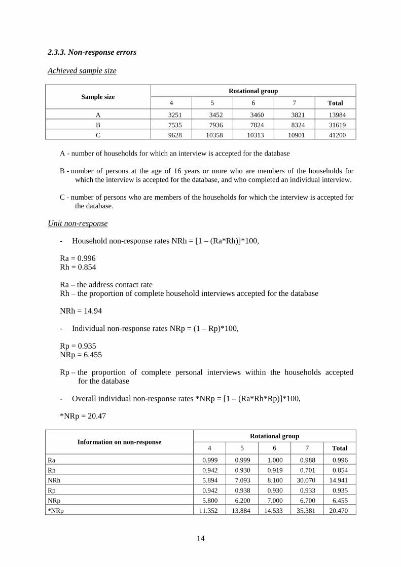
2.3.3. Non-response errors Achieved sample size

Rotational group Sample size

4 5 6 7 Total

A 3251 3452 3460 3821 13984

B 7535 7936 7824 8324 31619

C 9628 10358 10313 10901 41200

A - number of households for which an interview is accepted for the database B - number of persons at the age of 16 years or more who are members of the households for

which the interview is accepted for the database, and who completed an individual interview. C - number of persons who are members of the households for which the interview is accepted for

the database.

Unit non-response

- Household non-response rates NRh = [1 – (Ra*Rh)]*100, Ra = 0.996 Rh = 0.854 Ra – the address contact rate Rh – the proportion of complete household interviews accepted for the database NRh = 14.94 - Individual non-response rates NRp = (1 – Rp)*100, Rp = 0.935 NRp = 6.455 Rp – the proportion of complete personal interviews within the households accepted

for the database - Overall individual non-response rates *NRp = [1 – (Ra*Rh*Rp)]*100, *NRp = 20.47

Rotational group Information on non-response

4 5 6 7 Total

Ra 0.999 0.999 1.000 0.988 0.996

Rh 0.942 0.930 0.919 0.701 0.854

NRh 5.894 7.093 8.100 30.070 14.941

Rp 0.942 0.938 0.930 0.933 0.935

NRp 5.800 6.200 7.000 6.700 6.455

*NRp 11.352 13.884 14.533 35.381 20.470

15

Distribution of households

- DB120 - Contact at address

Rotational group DB120

4 5 6 7 Total

Address contacted (11) 3294 3543 3634 5251 15722

Address cannot be located (21) 2 1 1 59 63

Address impossible to access (22) 0 1 0 6 7

Address does not exist or is non-residential or is unoccupied or not the principal residence (23) 17 25 31 700 773

Total 3313 3570 3666 6016 16565

- DB130 - Household questionnaire result


4 5 6 7 Total

Household questionnaire completed (11) 3251 3452 3460 3823 13986

Refusal to co-operate (21) 116 139 217 1268 1740

Entire household temporarily away for duration of fieldwork (22) 66 77 68 203 414

Household unable to respond (illness, incapacity,…) (23) 13 28 12 138 191

Other reasons (24) 4 14 10 22 50

Total 3450 3710 3767 5454 16381

- DB135 - Household interview acceptance


4 5 6 7 Total

Interview accepted for database (1) 3251 3452 3460 3821 13984

Interview rejected (2) 0 0 0 2 2

Total 3251 3452 3460 3823 13986

16

Item non-response (income variables)

(A) (B) (C)

Item non-response % of households having received

an amount

% of households with missing

values

% of households with partial information

Total household gross income 34.78 6.56 58.40

Total disposable household income 69.82 6.38 23.71

Total disposable household income before social transfers other than old-age and survivor’s benefits 69.79 8.54 20.42

Total disposable household income before social transfers. including old-age and survivor’s benefits 61.88 12.01 15.17

Net income components at household level

HY040N 0.85 0.21 0.28

HY050N 19.46 0.41 0.36

HY060N 4.30 0.16 0.03

HY070N 3.85 0.11 0.00

HY080N 5.23 0.62 0.03

HY081N 2.26 0.17 0.00

HY090N 1.07 0.91 0.00

HY100N 1.06 2.38 0.00

HY110N 3.58 0.09 0.01

HY120N 50.24 5.71 0.00

HY130N 4.51 0.34 0.01

HY131N 1.02 0.07 0.00

HY140N 34.36 40.46 23.51

HY145N 33.05 3.58 0.06

Gross income components at household level

HY040G 1.13 0.21 0.00

HY050G 18.53 0.41 1.29

HY060G 4.30 0.16 0.03

HY070G 3,85 0,11 0,00

HY080G 5,23 0,62 0,03

HY081G 2,26 0,17 0,00

HY090G 0,42 0,91 0,65

HY100G 1,06 2,38 0,00

HY110G 3,22 0,09 0,36

HY120G 50,24 5,71 0,00

HY130G 4,51 0,34 0,01

HY131G 1.02 0.07 0.00

HY140G 34.14 40.25 24.10

17

Item non-response % of persons 16+ having received

an amount

% of persons 16+ with missing

values

% of persons 16+ with partial information

Net income components at personal level

PY010N 31.02 9.71 0.09

PY020N 8.16 3.37 1.30

PY021N 0.20 0.26 0.00

PY035N 2.42 0.69 0.00

PY050N 6.24 2.99 0.32

PY070N 6.27 1.54 0.00

PY080N 0.01 0.00 0.00

PY090N 2.20 0.48 0.01

PY100N 24.21 2.23 0.25

PY110N 1.12 0.18 0.00

PY120N 0.30 0.08 0.00

PY130N 5.51 0.59 0.01

PY140N 0.93 0.12 0.00

PY010N 31.02 9.71 0.09

PY020N 8.16 3.37 1.30

Gross income components at personal level

PY010G 14.68 9.71 16.43

PY020G 8.16 3.37 1.30

PY021G 0.20 0.26 0.00

PY030G 2.41 24.93 0.31

PY031G 2.39 24.64 0.00

PY035G 2.42 0.69 0.00

PY050G 5.38 1.95 3.21

PY070G 6.27 1.54 0.00

PY080G 0.00 0.00 0.01

PY090G 1.47 0.48 0.73

PY100G 14.51 2.23 9.94

PY110G 0.50 0.18 0.62

PY120G 0.19 0.08 0.12

PY130G 3.00 0.59 2.52

PY140G 0.93 0.12 0.00

PY200G 27.45 10.02 0.00

18

Adopted methods of income variable imputation Imputation is aimed at obtaining complete records at the level of target variables. Target variables do not simply reflect questionnaire variables and their calculation algorithm is often complicated, although it principally consists in aggregation. So it is necessary to decide what aggregation level the imputation should take place at. There are three possible options:

- the level of questionnaire variables, - the level of partly aggregated components, - the level of ready-calculated target variables.

Since the only formal requirement is to obtain imputed target variables, all the above options are permissible and practicable, depending on the specific character of variables. However, the most frequent practice is the imputation at the level of questionnaire variables. There are certain arguments for this approach, on condition that the quantity of data and calculation algorithm details allow for it without much complication. First of all, imputation at the lowest aggregation level can be desirable for the principal reasons related to the quality of imputation when:

- a target variable implies components of different character (i.e. taking different but rather predictable values, e.g. various social benefits, or dependent on a number of explanatory variables and thus easier to be modelled separately);

- target variables include many components and it is often the case that some of them have the missing items, while others – the correct ones which would be missed during the imputation of an aggregated variable.

Secondly, there are practical arguments for the imputation of disaggregated variables, as the same data serve as a basis for calculating national variables differing from the Eurostat’s target variables. Thus the imputation of disaggregated components may be required so as to ensure the imputed data needed for other calculations. The imputation at the target variable level is carried out only when the above circumstances do not occur or when it is easier to overcome the practical difficulties than to carry out the imputation of disaggregated data. There are several methods of component imputation. They can be classified as deterministic and stochastic methods. In case of deterministic methods the selected method and the set of explanatory variables (algorithm) clearly determine the imputation values for each record. In stochastic methods the imputation value is determined with the use of a random component. That is why it may happen that with the same algorithm and the same data file each algorithm realisation will give slightly different imputation values. Although the stochastic methods slightly increase estimator variance (introducing an additional random error component), they do not distort variance or original data distribution characteristics and allow for the correct estimation of random error. Deterministic imputation brings about variable variance reduction in the file and random error underestimation; it also distorts to a greater extent the correlation structure (increasing correlations with explanatory variables). According to item 2.7 of Regulation 1981/2003 it is recommended that for EU-SILC imputation the methods retaining distribution characteristics should be applied, which means the preference for the stochastic methods.

19

Out of the stochastic methods the following were used in the task presented here: - Hot-deck method

Random selection of a representative (donor) out of the correct records. If auxiliary categorizing variables are used in the hot-deck method, a random representative is selected out of the records showing adequate values of auxiliary variables. If it is not possible to find a donor with the equivalent values for all the auxiliary variables, the so called sequence approach is applied. The categorising variables were ranked from the most to the least significant ones. If there are no donors available, categorization is carried out with the subsequent explanatory variables being left out, starting from the least significant ones so as to obtain a subset containing donors.

- Stochastic regression imputation Auxiliary variables are the explanatory variables of the regression model. The model takes the linear form or the logarithmic transformation is used. It is fitted on the basis of the correct records. The imputed value (or its logarithm in the case of transformed models) is a sum of the theoretical value derived from the model and a randomly selected model residual. The set of records of which the residual is selected is restricted to those which are nearest to the record imputed for the theoretical value derived from the model. Out of the deterministic methods the following are applied:

- Regression deterministic imputation The theoretical value from the model is adopted as the imputation value.

- Deduction imputation The imputation value is directly determined on the basis of the relationships between variables. In the case of imputation at the target variable level or imputation of the most significant components of target variables, stochastic imputation is applied in order to retain the variable properties distribution as required by Regulation 1981/2003. The application of stochastic regression imputation requires a model which describes well the formation of a variable with relatively small variance of an error term and good statistical qualities. With high variance of an error term, there is a danger of getting accidental values which are not typical of the correct part of the dataset. That is why in the cases where, in accordance with the assumption referred to above, stochastic imputation is required, the hot-deck method is applied in preference to regression imputation. This is particularly justified when the number of records for imputation is rather low, or when the number of correct records is too small for a suitable model fitting. Stochastic regression imputation is most widely used for incomes from hired employment, as:

- it is an important category of income, declared by a significant rate of respondents which, if present, has a significant share in the total household’s income;

- this category can be successfully modelled with the use of the variables included in the questionnaire;

- there is a large (absolute) number of missing data, the percentage, however, being rather small; a large number of correct records make it possible to design a well-fitted model.

In case of incomes from hired employment stochastic regression imputation is applied to the majority of records with missing items, both those for which observations from the previous year are available (panel sample) and the new ones in the sample. In case of other income categories stochastic regression imputation is used as the basic imputation method when incomes of the same type for a given person/household are known from the previous year. If such income data from the previous year are not available, the hot-deck method is applied.

20

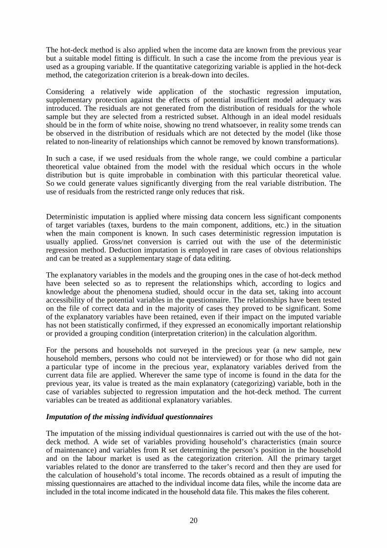
The hot-deck method is also applied when the income data are known from the previous year but a suitable model fitting is difficult. In such a case the income from the previous year is used as a grouping variable. If the quantitative categorizing variable is applied in the hot-deck method, the categorization criterion is a break-down into deciles. Considering a relatively wide application of the stochastic regression imputation, supplementary protection against the effects of potential insufficient model adequacy was introduced. The residuals are not generated from the distribution of residuals for the whole sample but they are selected from a restricted subset. Although in an ideal model residuals should be in the form of white noise, showing no trend whatsoever, in reality some trends can be observed in the distribution of residuals which are not detected by the model (like those related to non-linearity of relationships which cannot be removed by known transformations). In such a case, if we used residuals from the whole range, we could combine a particular theoretical value obtained from the model with the residual which occurs in the whole distribution but is quite improbable in combination with this particular theoretical value. So we could generate values significantly diverging from the real variable distribution. The use of residuals from the restricted range only reduces that risk. Deterministic imputation is applied where missing data concern less significant components of target variables (taxes, burdens to the main component, additions, etc.) in the situation when the main component is known. In such cases deterministic regression imputation is usually applied. Gross/net conversion is carried out with the use of the deterministic regression method. Deduction imputation is employed in rare cases of obvious relationships and can be treated as a supplementary stage of data editing. The explanatory variables in the models and the grouping ones in the case of hot-deck method have been selected so as to represent the relationships which, according to logics and knowledge about the phenomena studied, should occur in the data set, taking into account accessibility of the potential variables in the questionnaire. The relationships have been tested on the file of correct data and in the majority of cases they proved to be significant. Some of the explanatory variables have been retained, even if their impact on the imputed variable has not been statistically confirmed, if they expressed an economically important relationship or provided a grouping condition (interpretation criterion) in the calculation algorithm. For the persons and households not surveyed in the precious year (a new sample, new household members, persons who could not be interviewed) or for those who did not gain a particular type of income in the precious year, explanatory variables derived from the current data file are applied. Wherever the same type of income is found in the data for the previous year, its value is treated as the main explanatory (categorizing) variable, both in the case of variables subjected to regression imputation and the hot-deck method. The current variables can be treated as additional explanatory variables. Imputation of the missing individual questionnaires The imputation of the missing individual questionnaires is carried out with the use of the hot-deck method. A wide set of variables providing household’s characteristics (main source of maintenance) and variables from R set determining the person’s position in the household and on the labour market is used as the categorization criterion. All the primary target variables related to the donor are transferred to the taker’s record and then they are used for the calculation of household’s total income. The records obtained as a result of imputing the missing questionnaires are attached to the individual income data files, while the income data are included in the total income indicated in the household data file. This makes the files coherent.

21

Total item non-response and number of observations in the sample at unit level of common cross-sectional European indicators based on cross-sectional component of EU-SILC, for equivalised disposable income.

Indicator Achieved sample

size Total item non-

response

At-risk-of-poverty rate after social transfers - total 41200 14649

At-risk-of-poverty rate after social transfers - men total 19772 7256

At-risk-of-poverty rate after social transfers - women total 21428 7393

At-risk-of-poverty rate after social transfers - 0-17 years 8743 3126

At-risk-of-poverty rate after social transfers - 18-64 years 26462 10151

At-risk-of-poverty rate after social transfers - men 18-64 years 12923 5104

At-risk-of-poverty rate after social transfers - women 18-64 years 13539 5047

At-risk-of-poverty rate after social transfers - 65+ years 5995 1372

At-risk-of-poverty rate after social transfers - men 65+ years 2378 556

At-risk-of-poverty rate after social transfers - women 65+ years 3617 816

At-risk-of-poverty threshold - single 41200 14649

At-risk-of-poverty threshold - 2 adults, 2 children 41200 14649

Relative median at-risk-of-poverty gap - total 41200 14649

Relative median at-risk-of-poverty gap - men total 19772 7256

Relative median at-risk-of-poverty gap - women total 21428 7393

Relative median at-risk-of-poverty gap - 0-17 years 8743 3126

Relative median at-risk-of-poverty gap - 18-64 years 26462 10151

Relative median at-risk-of-poverty gap - men, 18-64 years 12923 5104

Relative median at-risk-of-poverty gap - women, 18-64 years 13539 5047

Relative median at-risk-of-poverty gap - 65+ years 5995 1372

Relative median at-risk-of-poverty gap - men, 65+ years 2378 556

Relative median at-risk-of-poverty gap - women, 65+ years 3617 816

Inequality of income distribution S80/S20 income quintile share ratio 41200 14649

In work at-risk-of-poverty rate - total 14558 5276

In work at-risk-of-poverty rate - men total 7914 2781

In work at-risk-of-poverty rate - women total 6644 2495

Relative median income ratio people aged 65+/0-64 41200 14649

Relative median income ratio people aged 65+/0-64 - men 19772 7256

Relative median income ratio people aged 65+/0-64 - women 21428 7393

Aggregate replacement ratio pensions 65-74/earnings 50-59 5593 2588

Aggregate replacement ratio pensions 65-74/earnings 50-59 - men 2842 1396

Aggregate replacement ratio pensions 65-74/earnings 50-59 - women 2751 1192

22

Indicator Achieved sample

size Total item non-

response

Before social transfers except old-age and survivors' benefits

At-risk-of-poverty rate before social transfers - total 41200 14091

At-risk-of-poverty rate before social transfers - men total 19772 6983

At-risk-of-poverty rate before social transfers - women total 21428 7108

At-risk-of-poverty rate before social transfers - 0-17 years 8743 2988


At-risk-of-poverty rate before social transfers - men, 18-64 years 12923 4911

At-risk-of-poverty rate before social transfers - women, 18-64 years 13539 4851

At-risk-of-poverty rate before social transfers - 65+ years 5995 1341

At-risk-of-poverty rate before social transfers - men, 65+ years 2378 544

At-risk-of-poverty rate before social transfers - women, 65+ years 3617 797


At-risk-of-poverty rate before social transfers - total 41200 13415

At-risk-of-poverty rate before social transfers - men total 19772 6671

At-risk-of-poverty rate before social transfers - women total 21428 6744



At-risk-of-poverty rate before social transfers - men, 18-64 years 12923 4753

At-risk-of-poverty rate before social transfers - women, 18-64 years 13539 4629

At-risk-of-poverty rate before social transfers - 65+ years 5995 1121

At-risk-of-poverty rate before social transfers - men, 65+ years 2378 438

At-risk-of-poverty rate before social transfers - women, 65+ years 3617 683

Mean equivalised disposable income 41200 14649

2.4. Mode of data collection EU-SILC is a non-obligatory, representative survey of individual households, performed by a face-to-face interview technique with the use of paper form questionnaires (the so called PAPI method). Two types of questionnaire: individual and household questionnaire are applicable.

23

Distribution of RB250 and RB260

- RB250 – Data status

Rotational group RB250

4 5 6 7 Total

Information completed only from interview (11) 7535 7936 7824 8324 31619

Individual unable to respond (illness, incapacity, etc) (21) 21 23 32 38 114

Refusal to co-operate (23) 239 283 281 319 1122

Person temporarily away and no proxy possible (31) 153 173 175 182 683

No contact for another reasons (32) 55 47 102 57 261

Information not completed: reason unknown (33) 0 1 0 1 2

Total 8003 10363 8324 8921 33801

- RB260 – Type of interview

Rotational group

RB260 4 5 6 7 Total

Face to face (1) 6101 6463 6387 6943 25894

Proxy interview (2) 1434 1473 1437 1381 5725

Total 7535 7936 7824 8324 31619

As for individual interviews, in 2008 a relatively high share (17,2%) of proxy interviews was noted. This was thoroughly discussed with the survey coordinators in the field. The interviewers decided on proxy interviews only if the substitute respondents were well informed about the situation in the household and there was no other possibility to get the information. Proxy interviews were performed in the following situations:

- no contact with the respondent because of long-term absence (e.g. work in another town or abroad);

- respondent’s disability, illness or pathology (such as alcoholism); - according to other members of the household, the respondent was only available late at

night and was not willing to participate in such a long interview, while at the same time the proxy could provide detailed information, even based on the documents, such as tax statements.

2.5. Interview duration The average household interview duration was about 33 minutes, while the average individual interview duration was about 22 minutes. In total the average time needed to carry out a household interview and individual interviews with persons at the age of 16 years and over was 83 minutes.

24

This value exceeded significantly that assumed in the regulation, which results from the fact that in the Polish SILC all the information is collected during the interview. The questionnaire parts covering social benefits and self-employment (in and outside farming) have been expanded by many auxiliary questions which help to answer but, on the other hand, prolong the interview. Problem of the interview duration was already pointed out in the Intermediate Quality Report for EU-SILC 2005 and 2006. 3. Comparability 3.1. Basic concepts and definitions The reference population

No difference to the common definition. The survey unit was a household and all the household members who had completed 16 years of age by December 31, 2007. The survey did not cover collective accommodation households (such as boarding house, workers’ hostel, pensioners’ house or monastery), except for the households of the staff members of these institutions living in these buildings in order to do their job (e.g. hotel manager, tender etc.). The households of foreign citizens should participate in the survey. The private household definition

No difference to the common definition. Household is a group of persons related to each other by kinship or not, living together and sharing their income and expenditure (multi-person household) or a single person, not sharing his/her income or expenditure with any other person, whether living alone or with other persons (one-person household). Family members living together but not sharing their income and expenditure with other family members make up separate households. The household size is determined by the number of persons comprised by the household. The household membership

No difference to the common definition. The household composition accounted for: - persons living together and sharing their income and expenditure who have been in the

household for at least 6 months (either the real or the intended time of staying in the household should be considered),

- persons absent from the household because of their occupation, if their earnings are allocated to the household’s expenditure,

- persons at the age of up to 15 years (inclusive), absent from the household for education purposes, living in boarding houses or private dwellings,

- persons absent from the household at the time of the survey, staying at education centres, welfare houses or hospitals, if their real or intended stay outside the household is less than 6 months.

25

The household composition did not account for: - persons at the age of over 15 years, absent from the household for education purposes,

living in boarding houses, students’ hostels or private dwellings, - men in military service (those performing substitute military service working

in companies and living at home are included in the household), - persons in prison, - persons absent from the household at the time of the survey, staying at education centres,

welfare houses or hospitals, if their real or intended stay outside the household is more than 6 months,

- persons (household’s guests) staying in the household at the time of the survey who have been or intended to be there for less than 6 months,

- persons renting a room, including students (unless they are treated as household members),

- persons renting a room or bed for the time of work in a given place (including such works as land melioration, geodetic measurements, forest cut-down or building constructions),

- persons living in the household and employed as au pairs, helping personnel on the farm, craft apprentices or trainees.

The income reference period(s) used

No difference to the common definition. The income reference period was last calendar year (2007). Reference period for taxes on income and social insurance contributions

The reference period for income tax prepayment and compulsory social insurance contributions is the year 2007. The account clearance with the Treasury Office (including payments and returns) effected in 2007 refers to the income for 2006. The reference period for taxes on wealth

No difference to the common definition. Taxes on wealth paid during the income reference period (2007) were recorded. The lag between the income reference period and current variables

The lag between the income reference period and current variables is about 5 months. The total duration of the data collection of the sample

EU-SILC was performed on the territory of the whole country between May 2 and June 26 2008. Basic information on activity status during the income reference period

No difference to the common definition.

26

3.2. Components of income 3.2.1. Differences between the national definitions and standards EU-SILC definitions, and an assessment: Total gross household income HY010 No difference to the common definition. Total disposable household incomeHY020 No difference to the common definition. Total disposable household income before social transfers except old-age and survivor` benefits HY022 No difference to the common definition. Total disposable household income before social transfers including old-age and survivor` benefits HY023 No difference to the common definition. In accordance with EU-SILC 065 (2008 operation) the new income components, mandatory from 2007 operation onwards:

� PY020G – NON-CASH EMPLOYEE INCOME; � PY030G – EMPLOYER'S SOCIAL INSURANCE CONTRIBUTION; � PY070G – VALUE OF GOODS PRODUCED FOR OWN CONSUMPTION; � PY080G – PENSION FROM INDIVIDUAL PRIVATE PLANS; � HY030G – IMPUTED RENT; � HY100G – INTEREST REPAYMENTS ON MORTGAGE

have been recorded at component level only and they are not included in the household`s total income (variables: HY010G; HY020G; HY22G; HY023G). Imputed rent HY030 This variable has been calculated in foothold about econometric model. Regular inter-household cash transfer received HY080 and regular inter-household cash transfer paid HY130 In EU-SILC2008 from both variables on regular cash transfers (HY080 and HY130) two additional variables were distinguished: Alimonies received - compulsory + voluntary (HY081), and Alimonies paid – compulsory + voluntary (HY131) . HY081 variable is contained the variable HY080 and similarly, HY131 is contained in HY130.

27

Employee cash or near cash income PY010 This variable does not account for: - assistance for foster families; since granting the benefit is not connected with quitting the job,

this benefit has been qualified to the category of „Family related allowances’ (HY050), - benefit granted to the families when the only person providing income for the family

is called up to the active military service; since this benefit is only granted when the only family supporter has been called to the military service, it has been included in the category of „Family related allowances’ (HY050).

Non-cash employee income PY020 Company car (PY021) – the information on the private use of the company car is collected in the individual questionnaire. Here belongs the respondent’s estimated amount he/she has gained by using the company car for private purposes. In case of the missing value (the respondent was using the company car but did not estimated the amount gained) imputation is applied with the use of hot-deck and regression imputation with simulated residuals methods; Cash benefits or losses from self-employment PY050 The data on income from self-employment were collected in two different ways: the respondents were asked about the company’s costs and profits and also about the amount of money gained from self-employment which was allocated to the household’s expenditure. After a detailed analysis of data it was decided that the income from self-employment would be equal to the amount allocated to the household’s needs. Survivors` benefits PY110 Death grants are not included in the income because the whole sum is used to cover the cost of the funeral. Sickness benefits PY120 Sickness and childcare benefits are not included (a childcare benefit is granted to the working parent of a sick child), because they are paid by the employer and cannot be detached from the income from hired employment. Therefore, they are accounted for in the income from hired employment. All the other variables not listed above Dwelling conditions and material deprivation items In 2007 the questions and guidelines for the interviewers referring to the dwelling conditions and material deprivation items were subject to the analysis. It was indicated that some records differed from those included in document 065/04:

28

Arrears on mortgage payment – it was not clarified that only arrears on mortgage should be taken into account, so other dwelling related credits might have been included. Arrears on hire purchase instalments other than loan payments – this question included arrears on hire purchase and credits other than dwelling-related ones. Capacity to afford paying for one week annual holiday away from home – first of all the question included the expression “if the household wants”; secondly, family as such was concerned and it was not pointed out that the question referred to the household as a whole. Leaking roof, damp walls/ floors/foundation, or rot in window frames or floor – the question was formulated in a different way, namely: “Do you think your dwelling requires renovation because of…?” Indoor flushing toilet for sole use of the household – the toilet could have been shared with other households. Additionally, for the variables from HS010 to HS050 no information was given that paying through borrowing meant that household was not in arrears. In EU-SILC 2008 amendments were introduced both in the questionnaire forms and in the guidelines for the interviewers, thus clearing up the differences. There were no other major divergences from common definitions. 3.2.2. The source or procedure used for the collection of income variables The income data were collected during the interviews with respondents. The target income variables were split into components corresponding to particular benefits applicable in the Polish conditions. 3.2.3. The form in which income variables at component level have been obtained The respondents were asked to give the net incomes and contributions (income tax prepayments and compulsory social insurance). Only in the case of income from rental of a property (HY040) the respondents were asked to give the gross income and the amount of tax paid. 3.2.4. The method used for obtaining income target variables in the required form The gross income was obtained by summing up net value, income tax prepayments and compulsory social insurance contributions. If the information on tax and insurance contributions was missing, the amounts were imputed on the basis of the results obtained. Only in the case of income from rental of property, the tax paid was subtracted from the gross income.

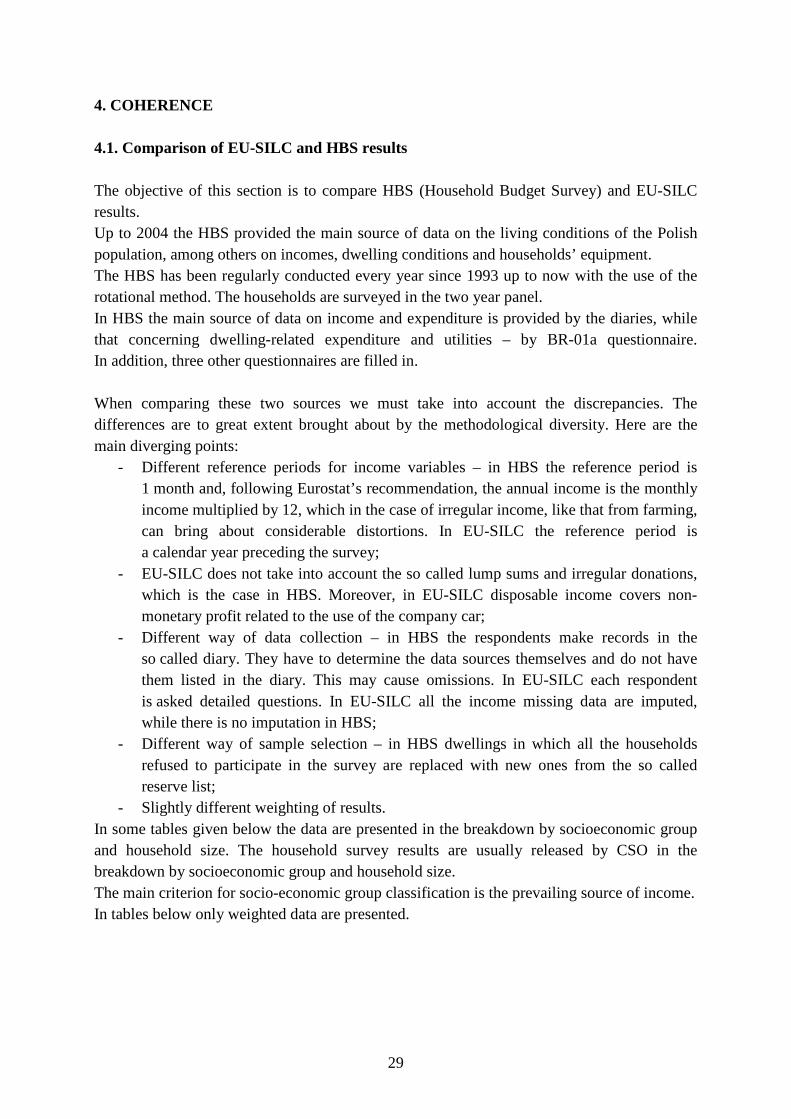
29

4. COHERENCE 4.1. Comparison of EU-SILC and HBS results The objective of this section is to compare HBS (Household Budget Survey) and EU-SILC results. Up to 2004 the HBS provided the main source of data on the living conditions of the Polish population, among others on incomes, dwelling conditions and households’ equipment. The HBS has been regularly conducted every year since 1993 up to now with the use of the rotational method. The households are surveyed in the two year panel. In HBS the main source of data on income and expenditure is provided by the diaries, while that concerning dwelling-related expenditure and utilities – by BR-01a questionnaire. In addition, three other questionnaires are filled in. When comparing these two sources we must take into account the discrepancies. The differences are to great extent brought about by the methodological diversity. Here are the main diverging points:

- Different reference periods for income variables – in HBS the reference period is 1 month and, following Eurostat’s recommendation, the annual income is the monthly income multiplied by 12, which in the case of irregular income, like that from farming, can bring about considerable distortions. In EU-SILC the reference period is a calendar year preceding the survey;

- EU-SILC does not take into account the so called lump sums and irregular donations, which is the case in HBS. Moreover, in EU-SILC disposable income covers non-monetary profit related to the use of the company car;

- Different way of data collection – in HBS the respondents make records in the so called diary. They have to determine the data sources themselves and do not have them listed in the diary. This may cause omissions. In EU-SILC each respondent is asked detailed questions. In EU-SILC all the income missing data are imputed, while there is no imputation in HBS;

- Different way of sample selection – in HBS dwellings in which all the households refused to participate in the survey are replaced with new ones from the so called reserve list;

- Slightly different weighting of results. In some tables given below the data are presented in the breakdown by socioeconomic group and household size. The household survey results are usually released by CSO in the breakdown by socioeconomic group and household size. The main criterion for socio-economic group classification is the prevailing source of income. In tables below only weighted data are presented.

30

Tab. 1. Structure of population by age

EU-SILC 2008 HBS 2008 Specification

in %

Total 100.0 100.0

0-14 15.7 18.1

15-24 15.1 15.8

25-54 44.0 41.6

55-64 11.8 12.1

65+ 13.5 12.4

Tab. 2. Structure of population by level of education


in %

Total 100.0 1000

No school education 1.9 0.7

Completed primary 16.4 17.0

Lower secondary 5.1 6.8

Elementary vocational 26.8 27.0

Secondary 34.4 34.5

Higher 15.4 14.0

Tab. 3. Structure of households and persons in households by socio-economic group

Households Persons in households Households

EU-SILC 2008 HBS 2007 EU-SILC 2008 HBS 2007

Total 13253090 13332283 37637658 37707821

Total = 100

Employees 52.3 47.5 62.7 56.3

Farmers 2.6 4.3 3.5 6.6

Self-employed 4.6 6.4 5.2 7.6

Retirees 27.4 27.6 18.6 18.9

Pensioners 8.4 9.2 5.2 6.4

Maintained from non-earned sources 4.8 5.0 4.7 4.2

31

Tab. 4. Average yearly equivalent income in PLN by socio-economic group

Disposable income Income from hired work Households


Total 18684 16549 11719 8857

Employees 20899 17120 17609 14287

Farmers 13550 16879 1356 1669

Self-employed 21348 23317 3201 3412

Retirees 15618 15089 1545 1694

Pensioners 12061 11472 1178 1234

Maintained from non-earned sources 9665 10327 2401 936

Tab. 5. Average yearly equivalent income in PLN by number of persons

Disposable income Income from hired work Households


Total 18684 16549 11719 8857

1-person 16883 15540 5675 4627

2-persons 21201 18849 9830 7426

3-persons 21001 18690 14861 11635

4-persons 19273 16936 14363 11036

5-persons 16238 14498 11012 8179

6-persons and more 14947 12605 9019 5679

Tab. 6. Households provided with selected durables


in %

Fixed telephone 68.5 64.2

Mobile telephone 79.9 83.5

Television set 97.5 98.5

Computer 54.5 56.4

Printer 40.0 37.1

Internet connection 43.0 45.6

Microwave oven 41.9 46.1

Dishwasher 11.5 9.6

Refrigerator 97.7 98.4

Washing machine 96.8 97.3

Passenger car 56.2 54.7

32

4.2. Comparison of Laeken Indicators based on EU-SILC 2007 and EU-SILC 2008 Preliminary explanations of the relative poverty range evaluation on the basis of SILC 2008 (based on the income condition in 2007) 1. In general the level of income poverty risk in 2007 was similar to that a year before. This is in agreement with the relative poverty figures estimated on the basis of HBS. 2. The decline in poverty gap reflects some improvement in the income condition of households, including those of lower income groups, which is also confirmed by a slight decrease of the income quintile share ratio. 3. By definition, the relative poverty rate informs us about changes in the income distribution. In 2007, as compared with 2006, the income position of the employees got better. For instance, the nominal income increased by almost 8% and the real income, by 5.5%. At the same time, retirement pays from the non-agricultural insurance system showed their nominal value increased by nearly 3%, while those of farmers, by slightly over 1%, which, in real terms, means some retirement pay reduction. In consequence, it was possible to note a relative deterioration in the income position of elderly people, which is revealed by an increased at-risk-of-poverty rate and lower aggregate replacement ratio and relative median income ratio of elderly people. 4. The favourable economic condition observed since 2004 accompanied by Poland’s joining the European Union had a stimulating effect on the labour market: the unemployment rate dropped, both real and nominal wages rose, the incomes of the self-employed, including farmers, got higher. This was reflected by the improved material condition of the Polish households, also the increasing income level and better material conditions (equipment with durable goods, better dwelling conditions). Therefore, a decline in the economic strain and durables indicator and a significant decline of at risk of poverty rate anchored at a fixed moment in time (2005) was observed. 4.3. Comparison between SNA results for the household sector and EU-SILC 2008 (data for 2007) in the scope of incomes The comparison covered disposable income and its main components: income from hired employment, self-employment (in and outside farming), as well as social benefits.

It was found out that the disposable income in EU-SILC 2008 made up 62% of the corresponding category in SNA. This was due to the following factors: 1. The household sector in SNA includes collective households which do not enter EU-SILC. 2. Both systems employ various methods of measuring income from self-employment. 3. Accounts of primary and secondary income distribution in SNA used for the determination of disposable income include some items not covered by EU-SILC 2008 or not taken into account in the calculation of its results. The most important of them are imputed rents.

33

In SNA income from self-employment is determined as the so called operation surplus which is the balance between the global production and current production inputs (i.e. intermediate consumption) and hired employees’ wages. This difference is reduced by taxes and increased by subsidies. The operation surplus thus calculated is allocated to the household’s consumer needs, housing-related investment as well as production-related investment. In the Polish EU-SILC the question about income from self-employment concerns just the amount allocated to the household’s consumer needs and its housing-related investment. In addition, SNA takes into account consumption from own production which is not taken into consideration by EU-SILC for farmers’ households. Due to these differences incomes from self-employment according to EU-SILC 2007 made 26% of the operation surplus only (after deduction of section K).

Incomes from hired employment in EU-SILC 2007 are equal to 101% of the corresponding figure in SNA, while social benefits – 92% respectively, which seems to be a good result. In EU-SILC 2008, as compared with EU-SILC 2007, the data coherence for disposable income with SNA increased by 4 percentage points. This is due to the coherence increase for income from hired employment by 2 percentage points, i.e. from 99% to 101%. In terms of value, wages and other incomes related to hired employment provide the most important component of disposable income in SNA. This category made up over 50% of the disposable income for 2007.

Taking into consideration the methodological changes in both surveys, the real increase of the coherence of income from hired employment was as high as 7 percentage points, rising from 95% to 102%. In EU-SILC 2008 RB050 weight was used for the calculation of individual incomes, while in EU-SILC 2007 – PB040, respectively. In SNA incomes of the employees working abroad were calculated in a different way. However, these methodological changes do not explain the increased coherence of incomes from hired employment. The change of weight in EU-SILC could justify an increase by 1 percentage point only. The methodological changes of SNA bring about reduced coherence between SNA data and EU-SILC data, since they lead to an increase in wages and other incomes from hired employment in SNA (for 2006 by over PLN 15 million). Considering the fact that SNA data are based on the results of the enterprise surveys, it can be judged that the increased coherence of incomes from hired employment might be due to some deterioration of the quality of enterprise survey results in the scope of wages. Unlike for EU-SILC 2006 and 2007, it is less probable that the increased coherence of SNA results in the area of hired employment could be brought about by a higher quality of EU-SILC results, as the coherence for all the other significant economic categories remained more or less at the same level.

The data coherence for social benefits between SNA and EU-SILC was 92%, and taking into account the change of the weighting method – 93%, which is equivalent to EU-SILC 2007.The coherence of income from self-employment between EU-SILC 2008 and SNA was 26% and taking into account the change of the weighting method – 27%, which is by 1 percentage point more than in EU-SILC 2007.

Comparison of 2007 results of SNA and EU-SILC 2008 for Poland

Category in SNA Variables

in EU-SILC 2008 Category description

in EU-SILC 2008

SNA in mln PLN

EU-SILC in mln PLN

SNA = 100%

SNA = 100%

EU-SILC 2007

Gross disposable income (net) HY020 Total disposable household income (net)

742 374 457 807 62 58

Wages, salaries and other income connected with hired work (gross)

PY010G Employee cash or near cash income (gross)

375 358 380 422 101 99

Gross operating surplus (gross) with the exception of section K

PY050G Self-employment income (gross) - value allocated to household’s consumption and dwelling-related investment

220 168 58 291 26 26

Social security benefits and social assistance benefits (gross)

PY90G + PY100G + PY110G + PY120G + PY130G + PY140G + HY050G + HY060G + HY070G

Social benefits (gross) 166 880 153 565 92 93

Remarks:

1. Remarks in brackets: “net” or “gross” refer to including or not including income tax and social security contributions, while the word “gross” in SNA names of categories refers to including of depreciation of fixed assets.

2. Data for gross operating surplus in SNA has been taken into consideration with the exception of section K, which allows for better comparability with EU-SILC data on self-employment income (PY050G). The data for section K includes mainly imputed rents, not included in the results of EU-SILC 2008 (data for 2007), and market income from renting of real estate included in EU-SILC as the variable HY040G.

SILC QRINT A PL 2008 0000 V0001 N - circabc.europa.eu... central statistical office of poland...

Documents

Transcript of SILC QRINT A PL 2008 0000 V0001 N - circabc.europa.eu... central statistical office of poland...