Significance of Cohen's Class for Time Frequency Analysis...

International Journal of Computer Applications (0975 – 8887)

Volume 72– No.12, June2013

1

Significance of Cohen's Class for Time Frequency Analysis of Signals

Azeemsha Thacham Poyil

College of Computers and Information Technology

Taif University, Saudi Arabia

Sultan Aljahdali College of Computers and

Information Technology Taif University, Saudi Arabia

Nasimudeen.K.M College of Computers and

Information Technology Taif University, Saudi Arabia

ABSTRACT

In this paper, a study of quadratic transformations under

Cohen‟s class is presented, to see the variations in resolution

for performing time-frequency analysis of signals. The study

concentrated on the analysis of linear chirp signals and non-

stationary signals in presence of noise as well as without

noise. The resolutions based on Wavelet Transform, Short

Time Fourier Transform are analysed. The effects of widow

length, wavelet scale and presence of noise are researched and

analyzed against the performance of different time-frequency

representations. The Cohen's class is a class of time-frequency

quadratic energy distributions which are covariant by

translations in time and in frequency. This important property

by the members of Cohen‟s class makes those representations

suitable for the analysis and detection of linear as well as

transient signals. Spectrogram, the squared modulus of Short

Time Fourier Transform is considered to be an element of

Cohen‟s class since it is quadratic and also co-variant in time

and frequency. Wigner Ville Distribution is another member

of Cohen‟s class which can be extended to many other

variants by changing the kernel functions used for cross-term

reductions. The trade-off in the time-frequency localization

are studied and demonstrated with the help of different plots.

The result of this study can be applied to enhance the

detection and analysis of signals and to develop efficient

algorithms in medical diagnosis as well as defense

applications.

Keywords

Wavelet Transform (WT), Scalogram, Short Time Fourier

Transform (STFT), Fast Fourier Transform (FFT), Wigner

Ville Distribution (WVD), Cohen‟s Class, Spectrogram

1. INTRODUCTION

The use of time-frequency techniques in signal analysis and

detection has been studied by many researchers at times. The

major reason for adopting these techniques in medical and

defense fields are the amount of simultaneous information we

get from this. In this paper a study of quadratic

transformations under Cohen‟s class is presented, to see the

variations in resolution for performing time-frequency

analysis of signals. The Cohen's class is a class of time-

frequency quadratic energy distributions which are covariant

by translations in time and in frequency [1]. The extraction of

useful data from a noisy multi-component signal is always a

big challenge for the researchers in the field of signal

processing. The concentration was on the study of linear chirp

signals and non-stationary signals using Wavelet Transform,

Scalogram, Spectrogram, STFT and Wigner Ville. For this

purpose many built-in MATLAB functions provided by the

Time-Frequency Toolbox have been used [1]. To start with,

some generic definitions and methods in time-frequency

signal analysis are described. After that, the need of time-

frequency representations is explained with the help of

examples. To the end of this paper, the results of many

transformations are plotted and explained for different types

and combinations of input signals.

2. BACKGROUND AND RELATED

WORK

2.1 STFT and Spectrogram

Short Time Fourier Transform is calculated for a signal by

pre-windowing the signal s(t) around a particular time t and

then calculating the Fourier transform [1]. And this is repeated

for all time instants t as in the equation 1.

duetuhustSTFT uj

x

2)()(),( (1)

Here h is the window function. The Spectrogram is defined as

the squared modulus of STFT and is by nature a

representation of the signal energy.

2

2)()(),(

duetuhustS uj

x

(2)

2.2 Wavelet Transform and Scalogram A continuous wavelet transform (CWT) is calculated by

projecting a signal s(t) on a family of zero-mean functions

called wavelets. The wavelets are deduced from a basic

function called mother wavelet by translations and dilations [1].

duuusatT atx )().();,( *

, (3)

Where

)(.)(2/1

,a

tuauat

(4)

The variable „a‟ is called scale factor. If the value of |a| is

greater than 1, in it dilates the wavelet and if the value of |a| is

less than 1 it compresses the wavelet. The major difference

between wavelet transform and STFT is that, when the scale

factor is changed, then both the duration and the bandwidth of

the wavelet are changed. But the shape of wavelet will be the



2

same as before. Another difference is that the WT uses short

windows at high frequencies and long windows at low

frequencies [1].

Scalogram of a signal s(t) is defined as the squared modulus

of the Continuous Wavelet Transform, which describes the

energy of the signal in time-scale plane.

2.3 Wigner Ville Distribution Wigner Ville Distribution (WVD) is a bilinear function of the

signal calculated using the formula,

detWVD j

s .. ) 2 -(t *s . ) 2 +s(t ),( 2

(5)

Where t represents time and ν represents frequency. One

major difference between the WVD and STFT is that the

calculation of WVD does not make use of any windows [1], [2].

2.4 Time and Frequency Marginal

A joint time and frequency energy density ),( tx is defined

in terms of the signal energy as

ddttE xx ,),(

(6)

Since the energy is a quadratic function of the signal, the

time-frequency energy distributions will also be in general

quadratic representations. The energy density parameter also

satisfies marginal properties as define below. Integrating the

energy density along one time axis will give rise to the energy

density corresponding to frequency and vice versa [1].

2)(),( Xdttx

(7)

2)(),( txdtx

(8)

Using the generic mathematical equations (7) and (8) for

quadratic distributions, the marginal of WVD along frequency

axis can be described by

2)(),( txdtWx

(9)

2)(),( XdttWx

(10)

2.5 Cohen’s Class Cohen‟s class of signals are generally represented by

).ds.d (s,).W- t,-(s);,( x tCs (11)

where, is known as smoothing function. So, the Cohen‟s

class can be defined as a smoothed version of the WVD. By

properly selecting the smoothing function we can create many

variants of WVD.

The spectrogram is an element of the Cohen's class since it is

quadratic, covariant with time and frequency, and also

preserves energy [1]. Spectrogram can be represented as a

smoothed version of WVD by selecting the smoothing

function as the „WVD of the window‟ function h.

As mentioned before, WVD is an element of Cohen's class

which can be understood by selecting the smoothing function

as a double Dirac function. The interference terms in WVD

can be effectively removed by selecting a suitable smoothing

kernel. There are many variants possible for WVD, for

example Smoothed WVD and Smoothed Pseudo WVD. Each

of them is implemented by selecting suitable smoothing

functions.

The pseudo WVD is defined as the frequency smoothed

version of the WVD according to the equation,

).d (t,).W(),( x HtPWVDx (12)

Here, )( H

is the Fourier transform of smoothing

window h(t). Here a compromise is done on many good

features of WVD in order to smooth out the cross terms.

Smoothed Pseudo WVD (SPWVD) is another variant in

Cohen‟s class which is implemented by splitting up the

smoothing function so as to provide an independent

smoothing in time domain as well as frequency domain. The

smoothing function can be represented as

)g(t).H(- ) (t, (13)

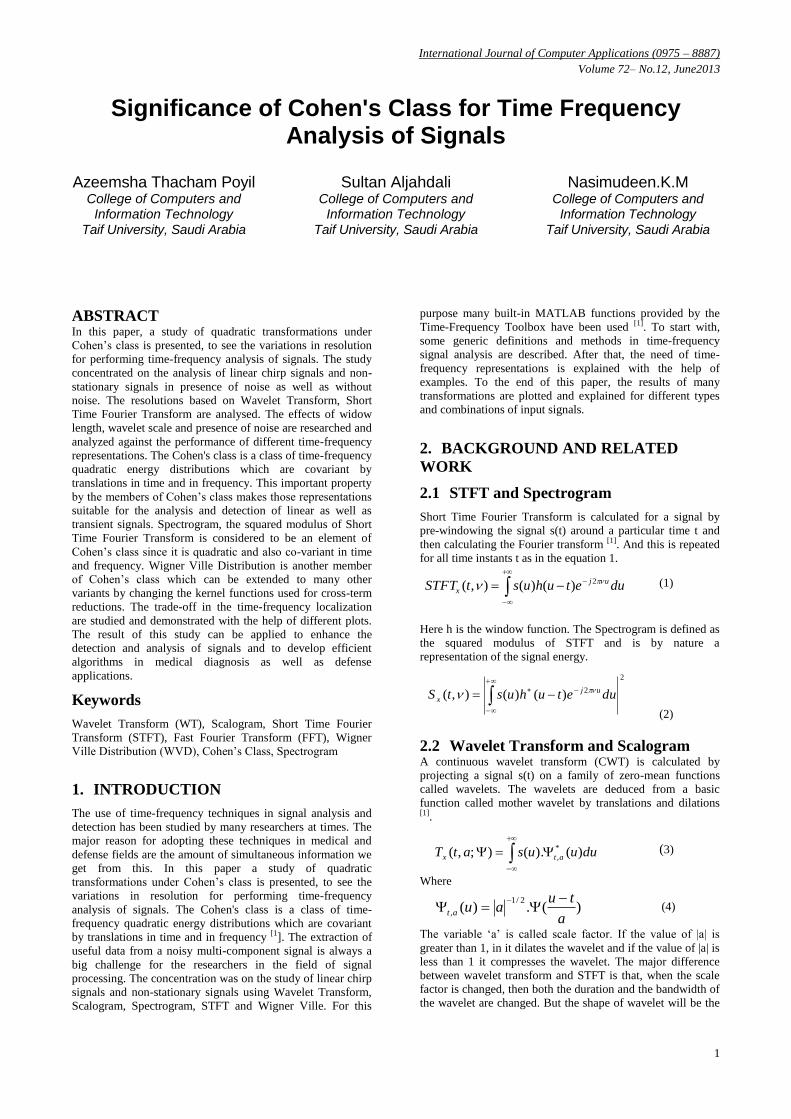
2.6 Time-Frequency resolution The need of simultaneous time-frequency localizations can be

understood using the below example. Figure 1 shows the

Gaussian modulated linear FM signal with an analytic

complex Gaussian noise with mean 0 and variance 1 added to

it. The FFT spectrum of the signal is also seen in the figure. It

is seen that the visibility of the signal spectrum is affected due

to the presence of noise. In order to map the time and

frequency information easily we can also look at the STFT

plot of the signal in the same figure.

Fig 1: STFT of the Noisy Signal

In the Figure 1 the wide colored area in the contour plot of the

signal‟s STFT represents the major signal component, and

some noise components spread away from that. It can be

noticed that the information we get from this plot helps us to

map between the frequency content and the time content of

the signal in the same plot. We can state which frequency

component exist at which point of time.

So it can be understood that the time-frequency representation

helps us to easily study and understand the frequency contents

of a signal at different time instants. Many researchers worked

in this area have produced lots of useful results towards

-1

-0.5

0

0.5

Real part

Signal in time

2004006008001000

Linear scale

Energ

y s

pectr

al density

|STFT|2, Lh=32, Nf=128, lin. scale, contour, Thld=5%

Time [s]

Fre

quency [

Hz]

50 100 150 200 2500

0.1

0.2

0.3

0.4

0.5



3

improving and comparing the performance. For example, N.

Zaric et al, did the implementation of a robust time-frequency

distribution for analysis of signals in presence of noise. This

included the development of an L-estimate STFT which uses

a sorting operation [3]. Another work by G. Yu proposed a

work on audio de-noising by using threshold in time-

frequency block [4]. Y. S. Wei and team researched on

algorithms for eliminating interference between signals and

thus helping multi-target signals in high frequency Radars [5].

Y.C.Jiang worked on generalized time–frequency

distributions for multi-component polynomial phase signals.

Three algorithms are proposed for removing the interference

terms in multi-component signals through the generalized

time–frequency distributions [6]. Yictor Sucic and team did

another study on optimization algorithm for selecting

quadratic Time-frequency Distributions in order to select the

distribution which provides the best localization of signal

components [7]. Daniel Mark Rosser researched on time-

frequency analysis of a carrier signal with additive white

Gaussian noise in order to help in signal detection problems,

which is addressed by time-frequency processing of the signal [8]. Boualem Boashash have extensively worked on time-

frequency signal analysis and processing proposing many

algorithms [9]. Higher order time-frequency poly-spectra are

studied by Alfred Hanssen and team [10]. Juan D Martinez-

Vargas et al have worked on time–frequency based algorithms

for feature extraction of transient bio-signals [11]. In another

research by Ervin Sejdic and associates, the time-frequency

features are studied by considering the energy concentration

as the parameter of analysis [12]. H. Zou et al had worked on

parametric time-frequency representations using translated

and dilated windowed exponential FM functions [13].

Hongxing Zou and team also worked on a similar area of

time–frequency distributions for parametric TFRs using

special class of transformation group called as „semi-affine‟

transformation group. This approach helps in achieving a

good visibility for highly non-stationary signals [14]. Jun Jason

Zhang et al proposed algorithms for time-frequency

characterization of signals in order to help in receiver

waveform design for shallow water environments [16].

Another research by B. Zhang and team discusses about the

time-frequency distribution of Cohen‟s class with a compound

kernel and its application in speech signal processing [17].

3. METHOD FOR ANALYSIS

For the study, many types and combinations of signals are

considered. As the first step, the representation of linear chirp

signals with and without the presence of noise was studied.

The WVD of the signal is calculated using the formula (5). In

the second step transient signals are studied with and without

the presence of noise. In the third step a LFM signal is

undergone rectangular amplitude modulation and then, the

STFT and Spectrogram are studied for different window

functions. The Wavelet Transform and Scalogram are studied

for „Altes Signal‟ in the next step. The time-frequency

resolution is compared against that achieved by using WVD.

To the end of the research, the cross-terms and time-frequency

localizations achieved using 3 variants of Cohen‟s class are

studied and compared.

4. RESULTS

The above methods are implemented in MATLAB using the

functions provided by Time Frequency Toolbox. After

applying the algorithms for quadratic representation of

different signals, a set of results as described are obtained.

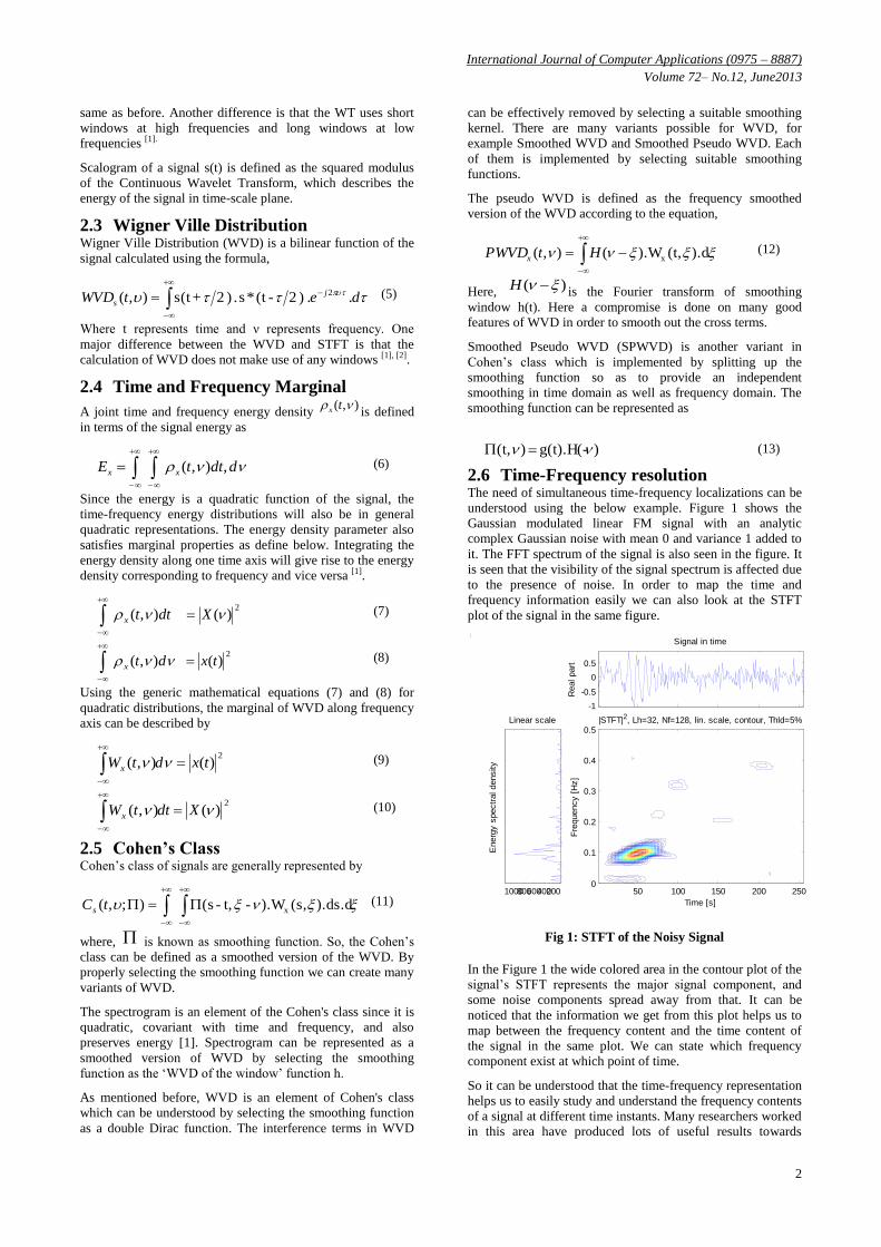
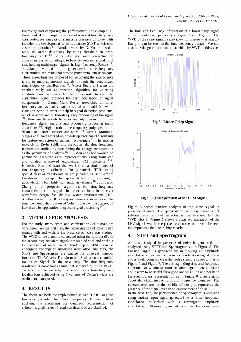
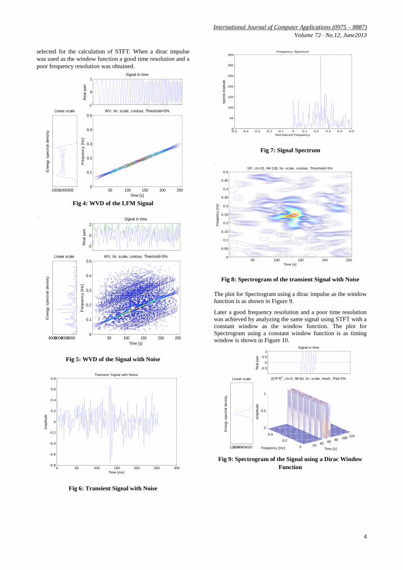
The time and frequency information of a linear chirp signal

are represented independently in Figure 2 and Figure 3. The

WVD of the same signal is also shown in Figure 4. A straight

line plot can be seen in the time-frequency domain. We can

also note the good localization provided by WVD in this case.

Fig 2: Linear Chirp Signal

Fig 3: Signal Spectrum of the LFM Signal

Figure 5 shows another analysis of the same signal in

presence of noise. The spectrum of the noisy signal is not

informative in terms of the actual and noise signal. But the

WVD plot in Figure 5 shows a clear representation of the

LFM signal even in the presence of noise. A line can be seen

that represents the linear chirp clearly.

4.1 STFT and Spectrogram

A transient signal in presence of noise is generated and

analyzed using STFT and Spectrogram as in Figure 8. The

transient signal is generated by multiplying an amplitude

modulation signal and a frequency modulation signal. Later

and analytic complex Gaussian noise signal is added to it as in

Figure 6 and Figure 7. The corresponding time and frequency

diagrams show almost unidentifiable signal details which

don‟t seem to be useful for a good analysis. On the other hand

the spectrogram representation as in Figure 8 gives a good

about the simultaneous time and frequency elements. The

concentrated area in the middle of the plot represents the

presence of the signal even in an environment of noise.

In the next step, the performance of Spectrogram is analyzed

using another input signal generated by a linear frequency

modulation multiplied with a rectangular amplitude

modulation. Different types of window functions were

0 50 100 150 200 250 300-1

-0.8

-0.6

-0.4

-0.2

0

0.2

0.4

0.6

0.8

1Linear FM Signal

Time

Am

plit

ude

-0.5 -0.4 -0.3 -0.2 -0.1 0 0.1 0.2 0.3 0.4 0.50

500

1000

1500Squared Spectrum of Signal

Normalized Frequency

Square

d M

odulu

s



4

selected for the calculation of STFT. When a dirac impulse

was used as the window function a good time resolution and a

poor frequency resolution was obtained.

Fig 4: WVD of the LFM Signal

Fig 5: WVD of the Signal with Noise

Fig 6: Transient Signal with Noise

Fig 7: Signal Spectrum

Fig 8: Spectrogram of the transient Signal with Noise

The plot for Spectrogram using a dirac impulse as the window

function is as shown in Figure 9.

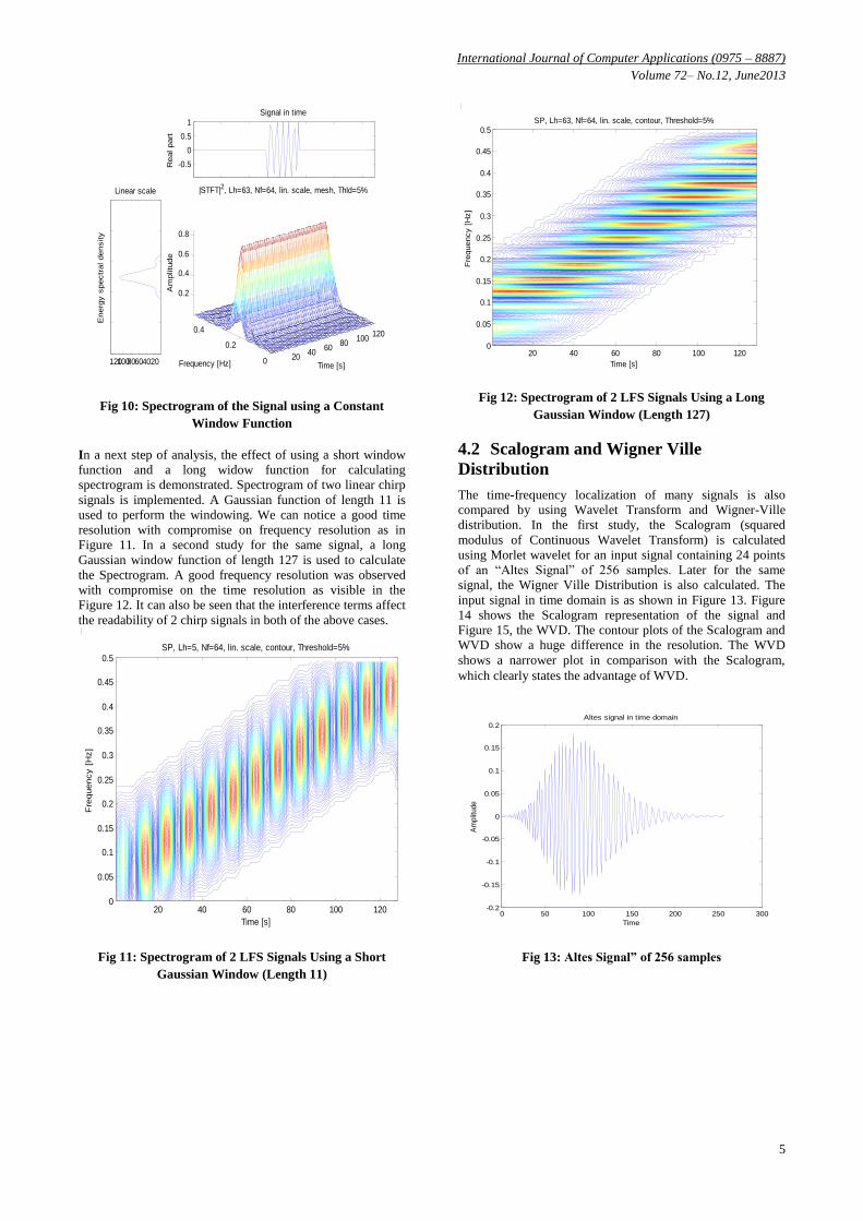
Later a good frequency resolution and a poor time resolution

was achieved by analyzing the same signal using STFT with a

constant window as the window function. The plot for

Spectrogram using a constant window function is as timing

window is shown in Figure 10.

Fig 9: Spectrogram of the Signal using a Dirac Window

Function

-1

0

1R

eal part

Signal in time

50010001500

Linear scale

Energ

y s

pectr

al density

WV, lin. scale, contour, Threshold=5%

Time [s]

Fre

quency [

Hz]

50 100 150 200 2500

0.1

0.2

0.3

0.4

0.5

-2

0

2

Real part

Signal in time

2000400060008000

Linear scale

Energ

y s

pectr

al density


Time [s]

Fre

quency [

Hz]

50 100 150 200 2500

0.1

0.2

0.3

0.4

0.5

0 50 100 150 200 250 300-0.8

-0.6

-0.4

-0.2

0

0.2

0.4

0.6

0.8Transient Signal with Noise

Time [ms]

Am

plit

ude

-0.5 -0.4 -0.3 -0.2 -0.1 0 0.1 0.2 0.3 0.4 0.50

50

100

150

200

250

300

350Frequency Spectrum

Normalized Frequency

Spe

ctra

l Am

plitu

de

SP, Lh=32, Nf=128, lin. scale, contour, Threshold=5%

Time [s]

Fre

quency [

Hz]

50 100 150 200 2500

0.05

0.1

0.15

0.2

0.25

0.3

0.35

0.4

0.45

0.5

-0.5

0

0.5

1

Real part

Signal in time

20406080100120

Linear scale

Energ

y s

pectr

al density

2040

6080

100120

0

0.2

0.4

0

0.5

1

Time [s]

|STFT|2, Lh=0, Nf=64, lin. scale, mesh, Thld=5%

Frequency [Hz]

Am

plit

ude



5

Fig 10: Spectrogram of the Signal using a Constant

Window Function

In a next step of analysis, the effect of using a short window

function and a long widow function for calculating

spectrogram is demonstrated. Spectrogram of two linear chirp

signals is implemented. A Gaussian function of length 11 is

used to perform the windowing. We can notice a good time

resolution with compromise on frequency resolution as in

Figure 11. In a second study for the same signal, a long

Gaussian window function of length 127 is used to calculate

the Spectrogram. A good frequency resolution was observed

with compromise on the time resolution as visible in the

Figure 12. It can also be seen that the interference terms affect

the readability of 2 chirp signals in both of the above cases.

Fig 11: Spectrogram of 2 LFS Signals Using a Short

Gaussian Window (Length 11)

Fig 12: Spectrogram of 2 LFS Signals Using a Long

Gaussian Window (Length 127)

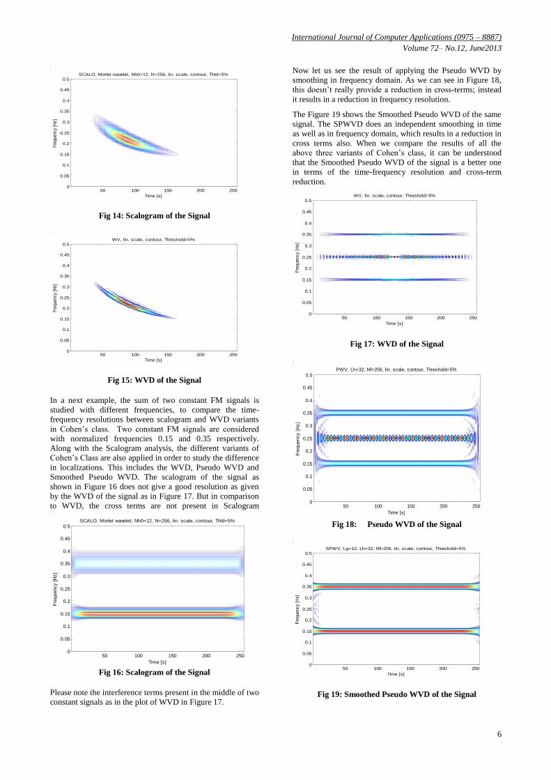
4.2 Scalogram and Wigner Ville

Distribution

The time-frequency localization of many signals is also

compared by using Wavelet Transform and Wigner-Ville

distribution. In the first study, the Scalogram (squared

modulus of Continuous Wavelet Transform) is calculated

using Morlet wavelet for an input signal containing 24 points

of an “Altes Signal” of 256 samples. Later for the same

signal, the Wigner Ville Distribution is also calculated. The

input signal in time domain is as shown in Figure 13. Figure

14 shows the Scalogram representation of the signal and

Figure 15, the WVD. The contour plots of the Scalogram and

WVD show a huge difference in the resolution. The WVD

shows a narrower plot in comparison with the Scalogram,

which clearly states the advantage of WVD.

Fig 13: Altes Signal” of 256 samples

-0.5

0

0.5

1

Real part

Signal in time

20406080100120

Linear scale

Energ

y s

pectr

al density

2040

6080

100120

0

0.2

0.4

0.2

0.4

0.6

0.8

Time [s]

|STFT|2, Lh=63, Nf=64, lin. scale, mesh, Thld=5%

Frequency [Hz]

Am

plitu

de


Time [s]

Fre

quency [

Hz]

20 40 60 80 100 1200

0.05

0.1

0.15

0.2

0.25

0.3

0.35

0.4

0.45

0.5


Time [s]

Fre

quency [

Hz]

20 40 60 80 100 1200

0.05

0.1

0.15

0.2

0.25

0.3

0.35

0.4

0.45

0.5

0 50 100 150 200 250 300-0.2

-0.15

-0.1

-0.05

0

0.05

0.1

0.15

0.2Altes signal in time domain

Time

Am

plit

ude



6

Fig 14: Scalogram of the Signal

Fig 15: WVD of the Signal

In a next example, the sum of two constant FM signals is

studied with different frequencies, to compare the time-

frequency resolutions between scalogram and WVD variants

in Cohen‟s class. Two constant FM signals are considered

with normalized frequencies 0.15 and 0.35 respectively.

Along with the Scalogram analysis, the different variants of

Cohen‟s Class are also applied in order to study the difference

in localizations. This includes the WVD, Pseudo WVD and

Smoothed Pseudo WVD. The scalogram of the signal as

shown in Figure 16 does not give a good resolution as given

by the WVD of the signal as in Figure 17. But in comparison

to WVD, the cross terms are not present in Scalogram


Please note the interference terms present in the middle of two

constant signals as in the plot of WVD in Figure 17.

Now let us see the result of applying the Pseudo WVD by

smoothing in frequency domain. As we can see in Figure 18,

this doesn‟t really provide a reduction in cross-terms; instead

it results in a reduction in frequency resolution.

The Figure 19 shows the Smoothed Pseudo WVD of the same

signal. The SPWVD does an independent smoothing in time

as well as in frequency domain, which results in a reduction in

cross terms also. When we compare the results of all the

above three variants of Cohen‟s class, it can be understood

that the Smoothed Pseudo WVD of the signal is a better one

in terms of the time-frequency resolution and cross-term

reduction.


Fig 18: Pseudo WVD of the Signal

Fig 19: Smoothed Pseudo WVD of the Signal

SCALO, Morlet wavelet, Nh0=12, N=256, lin. scale, contour, Thld=5%

Time [s]

Fre

quen

cy [

Hz]

50 100 150 200 2500

0.05

0.1

0.15

0.2

0.25

0.3

0.35

0.4

0.45

0.5


Time [s]

Fre

quen

cy [

Hz]

50 100 150 200 2500

0.05

0.1

0.15

0.2

0.25

0.3

0.35

0.4

0.45

0.5


Time [s]

Fre

quency [

Hz]

50 100 150 200 2500

0.05

0.1

0.15

0.2

0.25

0.3

0.35

0.4

0.45

0.5


Time [s]

Fre

quency [

Hz]

50 100 150 200 2500

0.05

0.1

0.15

0.2

0.25

0.3

0.35

0.4

0.45

0.5

PWV, Lh=32, Nf=256, lin. scale, contour, Threshold=5%

Time [s]

Fre

quency [

Hz]

50 100 150 200 2500

0.05

0.1

0.15

0.2

0.25

0.3

0.35

0.4

0.45

0.5

SPWV, Lg=12, Lh=32, Nf=256, lin. scale, contour, Threshold=5%

Time [s]

Fre

quency [

Hz]

50 100 150 200 2500

0.05

0.1

0.15

0.2

0.25

0.3

0.35

0.4

0.45

0.5



7

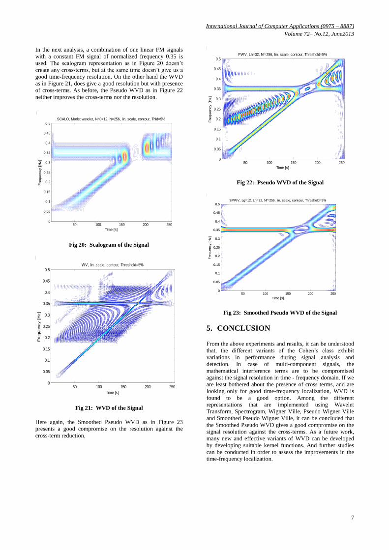
In the next analysis, a combination of one linear FM signals

with a constant FM signal of normalized frequency 0.35 is

used. The scalogram representation as in Figure 20 doesn‟t

create any cross-terms, but at the same time doesn‟t give us a

good time-frequency resolution. On the other hand the WVD

as in Figure 21, does give a good resolution but with presence

of cross-terms. As before, the Pseudo WVD as in Figure 22

neither improves the cross-terms nor the resolution.



Here again, the Smoothed Pseudo WVD as in Figure 23

presents a good compromise on the resolution against the

cross-term reduction.

Fig 22: Pseudo WVD of the Signal

Fig 23: Smoothed Pseudo WVD of the Signal

5. CONCLUSION

From the above experiments and results, it can be understood

that, the different variants of the Cohen‟s class exhibit

variations in performance during signal analysis and

detection. In case of multi-component signals, the

mathematical interference terms are to be compromised

against the signal resolution in time - frequency domain. If we

are least bothered about the presence of cross terms, and are

looking only for good time-frequency localization, WVD is

found to be a good option. Among the different

representations that are implemented using Wavelet

Transform, Spectrogram, Wigner Ville, Pseudo Wigner Ville

and Smoothed Pseudo Wigner Ville, it can be concluded that

the Smoothed Pseudo WVD gives a good compromise on the

signal resolution against the cross-terms. As a future work,

many new and effective variants of WVD can be developed

by developing suitable kernel functions. And further studies

can be conducted in order to assess the improvements in the

time-frequency localization.


Time [s]

Fre

quency [

Hz]

50 100 150 200 2500

0.05

0.1

0.15

0.2

0.25

0.3

0.35

0.4

0.45

0.5


Time [s]

Fre

quency [

Hz]

50 100 150 200 2500

0.05

0.1

0.15

0.2

0.25

0.3

0.35

0.4

0.45

0.5

PWV, Lh=32, Nf=256, lin. scale, contour, Threshold=5%

Time [s]

Fre

quency [

Hz]

50 100 150 200 2500

0.05

0.1

0.15

0.2

0.25

0.3

0.35

0.4

0.45

0.5

SPWV, Lg=12, Lh=32, Nf=256, lin. scale, contour, Threshold=5%

Time [s]

Fre

quency [

Hz]

50 100 150 200 2500

0.05

0.1

0.15

0.2

0.25

0.3

0.35

0.4

0.45

0.5



8

6. ACKNOWLEDGEMENT

The authors gratefully acknowledge the directions from the

MATLAB Time Frequency Toolbox for providing different

functions in order to perform the time-frequency

transformations, and thus helping the successful completion of

this research paper.

7. REFERENCES

[1] François Auger, Patrick Flandrin, Paulo Gonçalvès,

Olivier Lemoine, Tutorial - Time Frequency Toolbox for

use with MATLAB, 1996

[2] Azeemsha Thacham Poyil, Shadiya Alingal Meethal,

"Cross-term Reduction Using Wigner Hough Transform

and Back Estimation", IEEE Explore, Issue date 23-25

Aug. 2012

[3] N. Zaric, N. Lekic, and S. Stankovic, “An

implementation of the L-estimate distributions for

analysis of signals in heavy-tailed noise,” IEEE

Transactions on Circuits and Systems II, Vol. 58, No. 7,

July 2011, pp. 427-431

[4] G. Yu; S. Mallat, and E. Bacry, “Audio denoising by

time-frequency block thresholding,” IEEE Transactions

on Signal Processing, Vol. 56, No. 5, May 2008, pp.

1830-1839.

[5] Y. S. Wei and S. S. Tan, “Signal decomposition of HF

radar maneuvering targets by using S2-method with

clutter rejection,”Journal of Systems Engineering and

Electronics, Vol. 23, No. 2, April 2012, pp. 167 - 172.

[6] Y.C.Jiang, “Generalized time–frequency distributions for

multi-component polynomial phase signals,”Signal

Processing, Vol. 88, No. 4, April 2008, pp. 984–1001.

[7] Yictor Sucic and Boualem Boashash, “Optimization

Algorithm for Selecting Quadratic Time-frequency

Distributions: Performance Results and Calibration”

International Symposium on Signal Processing and its

Applications (ISSPA), Kuala Lumpur, Malaysia, 2001

[8] Daniel Mark Rosser, “Time-Frequency Analysis of a

Noisy Career Signal”, Naval Post Graduate School

Monterey, California, 1996

[9] Boualem Boashash, “Time-Frequency Signal Analysis

and Processing – A Comprehensive Reference”,

Queensland University of Technology, Brisbane,

Australia, 2003

[10] Alfred Hanssen, and Louis L. Scharf, “A Theory of

Polyspectra for Nonstationary Stochastic Processes”,

IEEE Transactions On Signal Processing, Vol. 51, No. 5,

2003

[11] Juan D Mart´ınez-Vargas, Juan I Godino-Llorente, and

German Castellanos-Dominguez, “Time–frequency

based feature selection for discrimination of non-

stationary biosignals”, EURASIP 2012

[12] Ervin Sejdic, Igor Djurovic and Jin Jiang, “Time-

Frequency Feature Representation Using Energy

Concentration: An Overview of Recent Advances”,

ScienceDirect, Digital Signal Processing 19 (2009) 153–

183

[13] H. Zou, Q. Dai, R. Wang, and Y. Li, “Parametric TFR

via windowed exponential frequency modulated atoms,”

IEEE Signal Processing Letters, Vol. 8, No. 5, May

2001,

[14] Hongxing Zou, Dianjun Wang, Xianda Zhang, Yanda Li,

“Nonnegative time–frequency distributions for

parametric time–frequency representations using semi-

affine transformation group”, Signal Processing 85

(2005)

[15] Time-series analysis in marine science and applications

for industry, 17– 21 September 2012 – Logonna-

Daoulas, France

[16] Jun Jason Zhang, Antonia Papandreou-Suppappola,

Bertrand Gottin, and Cornel Ioana, “Time-Frequency

Characterization and Receiver Waveform Design for

Shallow Water Environments”, IEEE Transactions On

Signal Processing, Vol. 57, No. 8, August 2009

[17] B. Zhang and S. Sato, “A time-frequency distribution of

Cohen‟s class with a compound kernel and its application

to speech signal processing,” IEEE Transactions on

Signal Processing, Vol. 42, No. 1, Jan. 1994, pp. 54-64.

Azeemsha Thacham Poyil, M Tech. He was born in Kerala,

India in 1979. He received his Bachelor degree in Electronics

and Communication Engineering from Kannur University,

India in 2001. Later he received his Master degree in

electronics from Cochin University of Science and

Technology, India in 2005. He is currently a Lecturer in

College of Computers and Information Technology, Taif

University, Saudi Arabia. He was previously working as

specialist software engineer with Bosch Thermo Technology,

Germany and Robert Bosch Engineering and Business

Solutions, India in the industrial product development. His

major research areas are Digital Signal Processing and

Embedded Systems.

Sultan Hamadi Aljahdali, PhD. He is graduated with Ph.D,

in Information Technology from George Mason University,

USA in 2003. He received his B.S from Winona State

University and M.S. with honor from Minnesota State

University in Mankato. He is currently an associate professor

in Dept. of Computer Science, Taif University. He is also the

dean of college of Computer & Information Technology, Taif

University Saudi Arabia. His research interests include

Performance Prediction in Software Engineering, Software

Modeling and Cost Estimation, Performance Modeling.

Nasimudeen.K.M, M.E (CS), M.C.A. He was born in Kerala,

India in 1979. He received his Bachelor degree in Electronics

from Kerala University, India in 2000. Later he received his

M.C.A(Master of Computer Application) degree from

Madurai Kamaraj University, Madurai, India in 2003 and he

obtained his M.E(Master of Engineering) degree in computer

science and Engineering from Anna University, Chennai in

2005. Pursuing his PhD in computer science and Engineering

from Anna University Chennai, India. Presently he is working

as a Lecturer in College of Computers and Information

Technology, Taif University, Taif, Kingdom of Saudi Arabia.

He was previously worked as Lecturer/HOD of Computer

Science department of Aalim Mohammed Salegh College of

Engineering, Chennai, India. His major research areas are

Natural language Processing and Neural network.

IJCATM : www.ijcaonline.org

Significance of Cohen's Class for Time Frequency Analysis...

Documents

Transcript of Significance of Cohen's Class for Time Frequency Analysis...