Identify the following signals Fouls and Signals Activities.

Signals and Systems 10EC44
Dept of ECE Alpha College of Engineering
SIGNALS & SYSTEMS (Common to EC/TC/IT/BM/ML)
Sub Code : 10EC44 IA Marks : 25
Hrs/ Week : 04 Exam Hours : 03
Total Hrs. : 52 Exam Marks : 100
UNIT 1:
Introduction: Definitions of a signal and a system, classification of signals, basic Operations on signals,
elementary signals, Systems viewed as Interconnections of operations, properties of systems. 6 Hrs
UNIT 2:
Time-domain representations for LTI systems – 1: Convolution, impulse response representation,
Convolution Sum and Convolution Integral. 6 Hrs
UNIT 3:
Time-domain representations for LTI systems – 2: Properties of impulse response representation,
Differential and difference equation Representations, Block diagram representations. 7 Hrs
UNIT 4:
Fourier representation for signals – 1: Introduction, Discrete time and continuous time Fourier series
(derivation of series excluded) and their properties . 7 Hrs
UNIT 5:
Fourier representation for signals – 2: Discrete and continuous Fourier transforms(derivations of
transforms are excluded) and their properties. 6 Hrs
UNIT 6:
Applications of Fourier representations: Introduction, Frequency response of LTI systems, Fourier
transform representation of periodic signals, Fourier transform representation of discrete time signals.
Sampling theorm and Nyquist rate. 7 Hrs
UNIT 7:
Z-Transforms – 1: Introduction, Z – transform, properties of ROC, properties of Z – transforms,
inversion of Z – transforms. 7 Hrs
UNIT 8:
Z-transforms – 2: Transform analysis of LTI Systems, unilateral Transform and its application to solve
difference equations. 6 Hrs

Signals and Systems 10EC44
Dept of ECE Alpha College of Engineering
TEXT BOOK
1. Simon Haykin, “Signals and Systems”, John Wiley India Pvt. Ltd., 2nd Edn, 2008.
2. Michael Roberts, “Fundamentals of Signals & Systems”, 2nd ed, Tata McGraw-Hill, 2010
REFERENCE BOOKS:
1. Alan V Oppenheim, Alan S, Willsky and A Hamid Nawab, “Signals and Systems” Pearson
Education Asia / PHI, 2nd edition, 1997. Indian Reprint 2002
2. H. P Hsu, R. Ranjan, “Signals and Systems”, Scham’s outlines, TMH, 2006
3. B. P. Lathi, “Linear Systems and Signals”, Oxford University Press, 2005
4. Ganesh Rao and Satish Tunga, “Signals and Systems”, Pearson/Sanguine Technical Publishers,
2004
Signals and Systems 10EC44
Dept of ECE Alpha College of Engineering
UNIT 1
INTRODUCTION
Learning Objectives:Introduction: Definitions of a signal and a system, classification of
signals, basic Operations on signals, elementary signals, Systems viewed as Interconnections of
operations, properties of systems.
Signal:
A signal is a function representing a physical quantity or variable, and typically it contains information
about the behaviour or nature of the phenomenon.
For instance, in a RC circuit the signal may represent the voltage across the capacitor or the current flowing
in the resistor. Mathematically, a signal is represented as a function of an independent variable ‘t’. Usually
‘t’represents time. Thus, a signal is denoted by x(t).
System:
A system is a mathematical model of a physical process that relates the input (or excitation)
signal to the output (or response) signal.
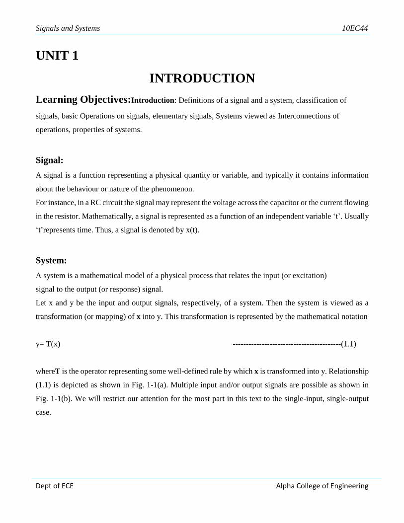
Let x and y be the input and output signals, respectively, of a system. Then the system is viewed as a
transformation (or mapping) of x into y. This transformation is represented by the mathematical notation
y= T(x) -----------------------------------------(1.1)
whereT is the operator representing some well-defined rule by which x is transformed into y. Relationship
(1.1) is depicted as shown in Fig. 1-1(a). Multiple input and/or output signals are possible as shown in
Fig. 1-1(b). We will restrict our attention for the most part in this text to the single-input, single-output
case.

Signals and Systems 10EC44
Dept of ECE Alpha College of Engineering
Fig1.1 :System with single or multiple input and output signals
Classification of signals :
Basically seven different classifications are there:
1. Continuous-Time and Discrete-Time Signals
2. Analog and Digital Signals
3. Real and Complex Signals
4. Deterministic and Random Signals
5. Even and Odd Signals
6. Periodic and Nonperiodic Signals
7. Energy and Power Signals
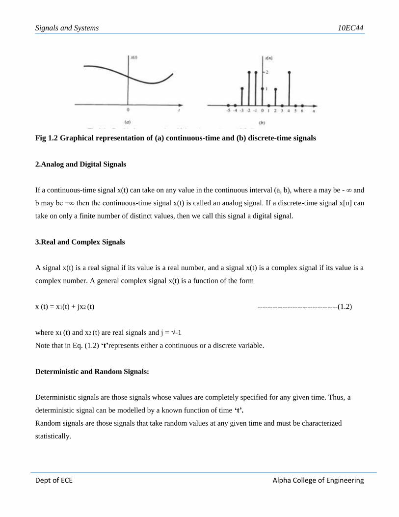
1.Continuous-Time and Discrete-Time Signals
A signal x(t) is a continuous-time signal if t is a continuous variable. If t is a discrete variable, that is, x(t)
is defined at discrete times, then x(t) is a discrete-time signal. Since a discrete-time signal is defined at
discrete times, a discrete-time signal is often identified as a sequence of numbers, denoted by {x,) or x[n],
where n = integer. Illustrations of a continuous- time signal x(t) and of a discrete-time signal x[n] are
shown in Fig. 1-2.
Signals and Systems 10EC44
Dept of ECE Alpha College of Engineering
Fig 1.2 Graphical representation of (a) continuous-time and (b) discrete-time signals
2.Analog and Digital Signals
If a continuous-time signal x(t) can take on any value in the continuous interval (a, b), where a may be - ∞ and
b may be +∞ then the continuous-time signal x(t) is called an analog signal. If a discrete-time signal x[n] can
take on only a finite number of distinct values, then we call this signal a digital signal.
3.Real and Complex Signals
A signal x(t) is a real signal if its value is a real number, and a signal x(t) is a complex signal if its value is a
complex number. A general complex signal x(t) is a function of the form
x (t) = x1(t) + jx2 (t) --------------------------------(1.2)
where x1 (t) and x2 (t) are real signals and j = √-1
Note that in Eq. (1.2) ‘t’represents either a continuous or a discrete variable.
Deterministic and Random Signals:
Deterministic signals are those signals whose values are completely specified for any given time. Thus, a
deterministic signal can be modelled by a known function of time ‘t’.
Random signals are those signals that take random values at any given time and must be characterized
statistically.

Signals and Systems 10EC44
Dept of ECE Alpha College of Engineering
Even and Odd Signals:
A signal x ( t ) or x[n] is referred to as an even signal if x (- t) = x(t)
x [-n] = x [n] -------------(1.3)
A signal x ( t ) or x[n] is referred to as an odd signal if x(-t) = - x(t)
x[- n] = - x[n]
--------------(1.4)
Examples of even and odd signals are shown in Fig. 1.3.
Figuer1.3 Examples of even signals (a and b) and odd signals (c and d).
Any signal x(t) or x[n] can be expressed as a sum of two signals, one of which is even and one of which is
odd. That is,
-------(1.5)

Signals and Systems 10EC44
Dept of ECE Alpha College of Engineering
Where,
-----(1.6)
Similarly for x[n],
X[n] = Xe[n] + Xo[n] -------(1.7)
Where,
Xe[n]=1/2{x[n] +x[-n]}
Xo[n]=1/2{x[n] -x[-n]} -------(1.8)
Note that the product of two even signals or of two odd signals is an even signal and that the product of an
even signal and an odd signal is an odd signal.
Periodic and Nonperiodic Signals :
A continuous-time signal x ( t ) is said to be periodic with period T if there is a positive nonzero value of T
for which
………(1.9)
An example of such a signal is given in Fig. 1-4(a). From Eq. (1.9) or Fig. 1-4(a) it follows that
---------------------------(1.10)
for all t and any integer m. The fundamental period T, of x(t) is the smallest positive value of
T for which Eq. (1.9) holds. Note that this definition does not work for a constant

Signals and Systems 10EC44
Dept of ECE Alpha College of Engineering
Figure 1.4 Examples of periodic signals.
signal x(t) (known as a dc signal). For a constant signal x(t) the fundamental period is undefined since x(t) is
periodic for any choice of T (and so there is no smallest positive value). Any continuous-time signal which is
not periodic is called a nonperiodic (or aperiodic) signal.
Periodic discrete-time signals are defined analogously. A sequence (discrete-time signal) x[n] is periodic with
period N if there is a positive integer N for which
……….(1.11)
An example of such a sequence is given in Fig. 1-4(b). From Eq. (1.11) and Fig. 1-4(b) it follows that
…………..(1.12)

Signals and Systems 10EC44
Dept of ECE Alpha College of Engineering
for all n and any integer m. The fundamental period No of x[n] is the smallest positive integer N for which
Eq.(1.11) holds. Any sequence which is not periodic is called a nonperiodic (or aperiodic sequence).
Note that a sequence obtained by uniform sampling of a periodic continuous-time signal may not be periodic.
Note also that the sum of two continuous-time periodic signals may not be periodic but that the sum of two
periodic sequences is always periodic.
Energy and Power Signals :
Consider v(t) to be the voltage across a resistor R producing a current i(t). The instantaneous power p(t) per
ohm is defined as
… ………(1.13)
Total energy E and average power P on a per-ohm basis are
……(1.14)
For an arbitrary continuous-time signal x (t), the normalized energy content E of x(t) is defined as
…………………(1.15)
The normalized average power P of x(t) is defined as
…………….(1.16)
Similarly, for a discrete-time signal x[n], the normalized energy content E of x[n] is defined as
…………….(1.17)
The normalized average power P of x[n] is defined as
…………….(1.18)

Signals and Systems 10EC44
Dept of ECE Alpha College of Engineering
Based on definitions (1.15) to (1.18), the following classes of signals are defined:
1. x(t) (or x[n]) is said to be an energy signal (or sequence) if and only if 0 < E < m, and so P = 0.
2. x(t) (or x[n]) is said to be a power signal (or sequence) if and only if 0 < P < m, thus implying that E = m.
3. Signals that satisfy neither property are referred to as neither energy signals nor power signals.
Note that a periodic signal is a power signal if its energy content per period is finite, and then the average
power of this signal need only be calculated over a period
Basic Operations on signals
The operations performed on signals can be broadly classified into two kinds
Operations on dependent variables
Operations on independent variables
Operations on dependent variables
The operations of the dependent variable can be classified into five types: amplitude scaling, addition,
multiplication, integration and differentiation.
Amplitude scaling
Amplitude scaling of a signal x(t) given by equation 1.19, results in amplification of
x(t) if a >1, and attenuation if a <1.
y(t) =ax(t) ……..(1.20)

Signals and Systems 10EC44
Dept of ECE Alpha College of Engineering
Figure 1.5 Amplitude scaling of sinusoidal signal
Addition
The addition of signals is given by equation of 1.21.
y(t) = x1(t) + x2 (t) ……(1.21)
Figure 1.6 Example of the addition of a sinusoidal signal with a signal of constant amplitude
Physical significance of this operation is to add two signals like in the addition of the background music along
with the human audio. Another example is the undesired addition of noise along with the desired audio signals.
Multiplication

Signals and Systems 10EC44
Dept of ECE Alpha College of Engineering
The multiplication of signals is given by the simple equation of 1.22.
y(t) = x1(t).x2 (t) ……..(1.22)
Figure 1.7 Example of multiplication of two signals
Differentiation
The operation of differentiation gives the rate at which the signal changes with respect to time, and can be
computed using the following equation, with Δt being a small interval of time.
If a signal doesnt change with time, its derivative is zero, and if it changes at a fixed rate with time, its
derivative is constant. This is evident by the example given in figure 1.8.

Signals and Systems 10EC44
Dept of ECE Alpha College of Engineering
Figure 1.8 Differentiation of Sine – Cosine
Operations on independent variables
Time scaling
Time scaling operation is given by equation 1.26
y(f) = x(af) ...............1.26
This operation results in expansion in time for a<l and com pressionintime for a>1.as evident from the ex amp1es
of figure 1.10.

Signals and Systems 10EC44
Dept of ECE Alpha College of Engineering
Figure 1.10 Examples of time scaling of a continuous time signal
An example of this operation is the compression or expansion of the time scale that results in the „fast-
forward’ or the „slow motion’ in a video, provided we have the entire video in some stored form.
Time reflection
Time reflection is given by equation (1.27), and some examples are contained in fig1.11.
y(t) = x(−t) ………..1.27
(a)

Signals and Systems 10EC44
Dept of ECE Alpha College of Engineering
(b)
Figure 1.11 Examples of time reflection of a continuous time signal
Time shifting
The equation representing time shifting is given by equation (1.28), and examples of this operation are given
in figure 1.12.
y(t) x(t- t0) ..............1.28

Signals and Systems 10EC44
Dept of ECE Alpha College of Engineering
Figure 1.12 Examples of time shift of a continuous time signal
Time shifting and scaling
The combined transformation of shifting and scaling is contained in equation (1.29), along with examples in
figure 1.13. Here, time shift has a higher precedence than time scale.
y(t) x(at –t0) .................1.29
t{time in seconds} t (time in seconds} t {time in seconds)
(a)

Signals and Systems 10EC44
Dept of ECE Alpha College of Engineering
(b)
Figure 1.13 Examples of simultaneous time shifting and scaling. The signal has to be shifted first
and then time scaled.
Elementary signals
Exponential signals:
The exponential signal given by equation (1.29), is a monotonically increasing function if
a> 0, and is a decreasing function if a < 0.
……………………(1.29)
It can be seen that, for an exponential signal,
…………………..(1.30)
Hence, equation (1.30), shows that change in time by ±1/ a seconds, results in change in magnitude by e±1 .
The term 1/ a having units of time, is known as the time-constant. Let us consider a decaying exponential
signal
……………(1.31)

Signals and Systems 10EC44
Dept of ECE Alpha College of Engineering
This signal has an initial value x(0) =1, and a final value x(∞) = 0 . The magnitude of this signal at five times
the time constant is,
…………….(1.32)
while at ten times the time constant, it is as low as,
……………(1.33)
It can be seen that the value at ten times the time constant is almost zero, the final value of the signal. Hence,
in most engineering applications, the exponential signal can be said to have reached its final value in about ten
times the time constant. If the time constant is 1 second, then final value is achieved in 10 seconds!! We have
some examples of the exponential signal in figure 1.14.
The sinusoidal signal:

Signals and Systems 10EC44
Dept of ECE Alpha College of Engineering
The sinusoidal continuous time periodic signal is given by equation 1.34, and examples are given in figure 1015
The different parameters are: Angular frequency co 2nfin radians,
Frequency fin Hertz, (cycles per second) Amplitude A in Volts (or Amperes) Period Tin seconds
The complex exponential:
We now represent the complex exponential using the Euler's identity
………….(1.35)
to represent sinusoidal signals. We have the complex exponential signal given by equation (1.36)
………(1.36)
Since sine and cosine signals are periodic, the complex exponential is also periodic with the same period as
sine or cosine. From equation (1.36), we can see that the real periodic sinusoidal signals can be expressed as:
Let us consider the signal x(t) given by equation (1.38). The sketch of this is given in fig 1.15
………………..(1.37)
…………………..(1.38)

Signals and Systems 10EC44
Dept of ECE Alpha College of Engineering
The unit impulse:
The unit impulse usually represented as δ (t) , also known as the dirac delta function, is given by,
…….(1.38)
From equation (1.38), it can be seen that the impulse exists only at t = 0 , such that its area is 1. This is a
function which cannot be practically generated. Figure 1.16, has the plot of the impulse function

Signals and Systems 10EC44
Dept of ECE Alpha College of Engineering
The unit step:
The unit step function, usually represented as u(t) , is given by,
……………….(1.39)

Signals and Systems 10EC44
Dept of ECE Alpha College of Engineering
Fig 1.17 Plot of the unit step function along with a few of its transformations
The unit ramp:
The unit ramp function, usually represented as r(t) , is given by,
……………(1.40)

Signals and Systems 10EC44
Dept of ECE Alpha College of Engineering
Figure1.18 Plot of the unit ramp function
The signum function:
The signum function, usually represented as sgn(t) , is given by
000 000000000 000000000 …………(1.41)

Signals and Systems 10EC44
Dept of ECE Alpha College of Engineering
Figure 1.19 Plot of the unit signum function along with a few of its transformations
1.5 System viewed as interconnection of operation:
This article is dealt in detail again in chapter 2/3. This article basically deals with system connected in series or
paralleL Further these systems are connected with adders/subtractor, multipliers etc.
1.6 Properties of system:
In this article discrete systems are taken into account. The same explanation stands for continuous time systems
also.
The discrete time system:
The discrete time system is a device which accepts a discrete time signal as its input,
transforms it to another desirable discrete time signal at its output.

Signals and Systems 10EC44
Dept of ECE Alpha College of Engineering
Stability
A system is stable if 'bounded input results in a bounded output'. This condition, denoted by BIBO,
Hence, a finite input should produce a finite output, if the system is stable. Some examples of stable and
unstable systems are given in figure 1.21
Memory
The system is memory-less if its instantaneous output depends only on the current input. In memory-less
systems, the output does not depend on the previous or the future input
Causality:
A system is causal, if its output at any instant depends on the current and past values of input. The
output of a causal system does not depend on the future values of input.
Invertibility:
A system is invertible if,
Linearity:
The system is a device which accepts a signal, transforms it to another desirable signal, and is available
at its output. We give the signal to the system, because the output is s

Signals and Systems 10EC44
Dept of ECE Alpha College of Engineering
Time invariance:
A system is time invariant, if its output depends on the input applied, and not on the time of application
of the input. Hence, time invariant systems, give delayed outputs for delayed inputs.

Signals and Systems 10EC44
Dept of ECE Alpha College of Engineering
UNIT 2
Time-domain representations for LTI systems – 1
Learning Objectives:Time-domain representations for LTI systems – 1: Convolution, impulse
response representation, Convolution Sum and Convolution Integral.
Introduction:
The Linear time invariant (LTI) system:
Systems which satisfy the condition of linearity as well as time invariance are known as linear time
invariant systems. Throughout the rest of the course we shall be dealing with LTI systems. If the output
of the system is known for a particular input, it is possible to obtain the output for a number of other
inputs. We shall see through examples, the procedure to compute the output from a given input-output
relation, for LTI systems.
Convolution:
Signals and Systems 10EC44
Dept of ECE Alpha College of Engineering
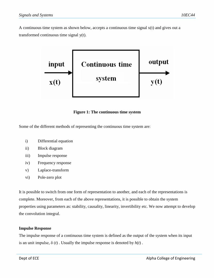
A continuous time system as shown below, accepts a continuous time signal x(t) and gives out a
transformed continuous time signal y(t).
Figure 1: The continuous time system
Some of the different methods of representing the continuous time system are:
i) Differential equation
ii) Block diagram
iii) Impulse response
iv) Frequency response
v) Laplace-transform
vi) Pole-zero plot
It is possible to switch from one form of representation to another, and each of the representations is
complete. Moreover, from each of the above representations, it is possible to obtain the system
properties using parameters as: stability, causality, linearity, invertibility etc. We now attempt to develop
the convolution integral.
Impulse Response
The impulse response of a continuous time system is defined as the output of the system when its input
is an unit impulse, δ (t) . Usually the impulse response is denoted by h(t) .

Signals and Systems 10EC44
Dept of ECE Alpha College of Engineering
Figure 2: The impulse response of a continuous time system
Convolution Sum:
We now attempt to obtain the output of a digital system for an arbitrary in input x[n], from the
knowledge of the system impulse response h[n].
y[n] = x[n]* h[n]
Convolution Integral:

Signals and Systems 10EC44
Dept of ECE Alpha College of Engineering
We now attempt to obtain the output of a continuous time/Analog digital system for an arbitrary input
x(t), from the knowledge of the system impulse response h(t), and the properties of the impulse response
of an LTI system.
Methods of evaluating the convolution integral: (Same as Convolution sum)
Given the system impulse response h(t), and the input x(t), the system output y(t), is given by the
convolution integral:

Signals and Systems 10EC44
Dept of ECE Alpha College of Engineering
Some of the different methods of evaluating the convolution integral are: Graphical representation,
Mathematical equation, Laplace-transforms, Fourier Transform, Differential equation, Block diagram
representation, and finally by going to the digital domain.

Signals and Systems 10EC44
Dept of ECE Alpha College of Engineering
Unit 3
Time-Domain Representations For LTI Systems – 2
Learning Objectives:Time-domain representations for LTI systems – 2: Properties of
impulse response representation, Differential and difference equation Representations, Block diagram
representations.
Time domain representation of LTI Systems
•Impulse response: characterizes the behavior of any LTI system
•Linear constant coefficient differential or difference equation: input output behavior
•Block diagram: as an interconnection of three elementary operations
Differential and Difference equation
•General form of differential equation is

Signals and Systems 10EC44
Dept of ECE Alpha College of Engineering

Signals and Systems 10EC44
Dept of ECE Alpha College of Engineering

Signals and Systems 10EC44
Dept of ECE Alpha College of Engineering

Signals and Systems 10EC44
Dept of ECE Alpha College of Engineering
Block diagram representations
•A block diagram is an interconnection of elementary operations that act on the input signal
•This method is more detailed representation of the system than impulse response or
differential/difference equation representations
•The impulse response and differential/difference equation descriptions represent only the input-output
behavior of a system, block diagram representation describes how the operations are ordered
•Each block diagram representation describes a different set of internal computations used to determine
the system output

Signals and Systems 10EC44
Dept of ECE Alpha College of Engineering
•Block diagram consists of three elementary operations on the signals:
– Scalar multiplication: y(t) = cx(t) or y[n] = x[n], where c is a
scalar
– Addition: y(t) = x(t)+w(t) or y[n] = x[n]+w[n].
•Block diagram consists of three elementary operations on the signals
Integration for continuous time LTI system:
Time shift for discrete time LTI system: y[n] = x[n−1]
•Scalar multiplication: y(t) = cx(t) or y[n] = x[n], where c is a scalar
Signals and Systems 10EC44
Dept of ECE Alpha College of Engineering
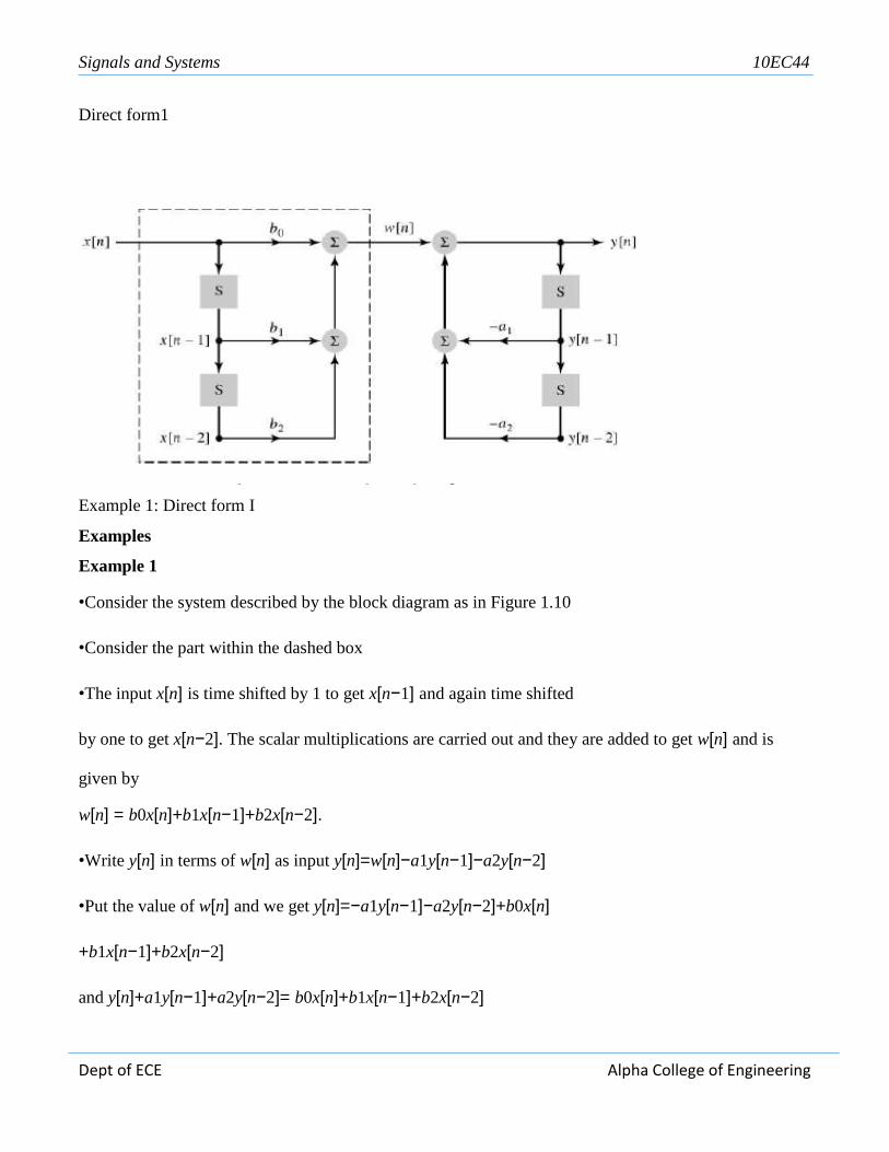
Direct form1
Example 1: Direct form I
Examples
Example 1
•Consider the system described by the block diagram as in Figure 1.10
•Consider the part within the dashed box
•The input x[n] is time shifted by 1 to get x[n−1] and again time shifted
by one to get x[n−2]. The scalar multiplications are carried out and they are added to get w[n] and is
given by
w[n] = b0x[n]+b1x[n−1]+b2x[n−2].
•Write y[n] in terms of w[n] as input y[n]=w[n]−a1y[n−1]−a2y[n−2]
•Put the value of w[n] and we get y[n]=−a1y[n−1]−a2y[n−2]+b0x[n]
+b1x[n−1]+b2x[n−2]
and y[n]+a1y[n−1]+a2y[n−2]= b0x[n]+b1x[n−1]+b2x[n−2]

Signals and Systems 10EC44
Dept of ECE Alpha College of Engineering
•The block diagram represents an LTI system
Example 2
•Consider the system described by the block diagram and its difference
equation is y[n]+(1/2)y[n−1]−(1/3)y[n−3]= x[n]+2x[n−2]
Example 3
•Consider the system described by the block diagram and its difference
equation is y[n]+(1/2)y[n−1]+(1/4)y[n−2]= x[n−1]
Block diagram representation is not unique, direct form II structure of
Example 1
•We can change the order without changing the input output behavior
Let the output of a new system be f [n] and given input x[n] are related
by
f[n] = −a1 f [n−1]−a2 f [n−2]+x[n]
•The signal f [n] acts as an input to the second system and output of
second system is
y[n] = b0 f [n]+b1 f [n−1]+b2 f [n−2].

Signals and Systems 10EC44
Dept of ECE Alpha College of Engineering
•The block diagram representation of an LTI system is not unique
Example 2: Direct form I
Direct form II

Signals and Systems 10EC44
Dept of ECE Alpha College of Engineering
UNIT 4
Fourier Representation for Signals – 1
Learning Objectives: Introduction, Discrete time and continuous time Fourier series (derivation
of series excluded) and their properties .
INTRODUCTION
In 1807, Jean Baptiste Joseph Fourier Submitted a paper of using trigonometric series to represent “any”
periodic signal. But Lagrange rejected it!
• In 1822, Fourier published a book “The Analytical Theory of Heat”
• Fourier’s main contributions: Studied vibration, heat diffusion, etc. and found that a series of
harmonically related sinusoids is useful in representing the temperature distribution through a body.
• He also claimed that “any” periodic signal could be represented by Fourier series.
• These arguments were still imprecise and it remained for P.L.Dirichlet in 1829 to provide precise
conditions under which a periodic signal could be represented by a FS.
• He however obtained a representation for aperiodic signals i.e., Fourier integral or transform
• Fourier did not actually contribute to the mathematical theory of Fourier series.
• Hence out of this long history what emerged is a powerful and cohesive framework for the analysis of
continuous- time and discrete-time signals and systems
• And an extraordinarily broad array of existing and potential application.
• Let us see how this basic tool was developed and some important Applications
Key Properties: for Input to LTI System
1. To represent signals as linear combinations of basic signals.

Signals and Systems 10EC44
Dept of ECE Alpha College of Engineering
2. Set of basic signals used to construct a broad class of signals.
3. The response of an LTI system to each signal should be simple enough in structure.
4. It then provides us with a convenient representation for the response of the system.
5. Response is then a linear combination of basic signal
Eigenfunctions and Values
• One of the reasons the Fourier series is so important is that it represents a signal in terms of
eigenfunctions of LTI systems.
• When I put a complex exponential function like x(t) = ejωtthrough a linear time-invariant system, the
output is y(t) = H(s)x(t) = H(s) ejωtwhere H(s) is a complex constant (it does not depend on time).
• The LTI system scales the complex exponential ejωt
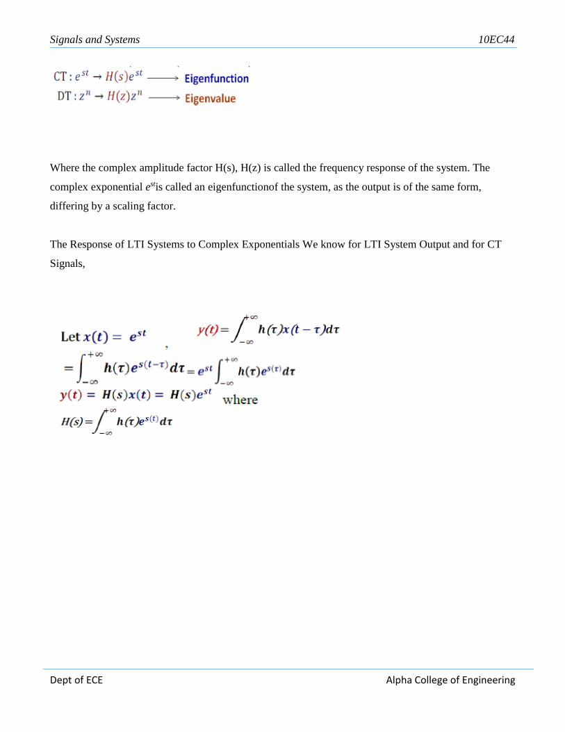
The Response of LTI Systems to Complex Exponentials
Let us analyse how an LTI system responds to complex signals
The Response of an LTI System:
For CT (Continuous Times) and DT (Discrete Times) we can say that
Signals and Systems 10EC44
Dept of ECE Alpha College of Engineering
Where the complex amplitude factor H(s), H(z) is called the frequency response of the system. The
complex exponential estis called an eigenfunctionof the system, as the output is of the same form,
differing by a scaling factor.
The Response of LTI Systems to Complex Exponentials We know for LTI System Output and for CT
Signals,

Signals and Systems 10EC44
Dept of ECE Alpha College of Engineering
Eigenfunction and Superposition Properties

Signals and Systems 10EC44
Dept of ECE Alpha College of Engineering
• Each system has its own constant H(s) that describes how it scales eigenfunctions. It is called the
frequency response.
• The frequency response H(ω)=H(s) does not depend on the input.
• If we know H(ω), it is easy to find the output when the input is an eigenfunction. y(t)=H(ω)x(t) true
when x is eigenfunction.
• So, given the system response to an eigenfunction, H(s), we can compute the magnitude response |H(s)|
and the phase response H(s).
• These form the scaling factor and phase shift in the output, respectively.
• The frequency of the output sinusoid will be the same as the frequency of the input sinusoid in any LTI
system.
• The LTI system scales and shifts sinusoids for both continuous and discrete signals and systems.
Need for Frequency Analysis
Fast & efficient insight on signal’s building blocks.
Simplifies original problem - ex.: solving Part. Diff. Eqns.
Powerful & complementary to time domain analysis techniques.
Several transforms in DSPing: Fourier, Laplace, z, etc.
Fourier Analysis : T

Signals and Systems 10EC44
Dept of ECE Alpha College of Engineering
The following are its Applications Telecommunication- GSM/cellular phones, Electronics/IT - most DSP-
based applications, Entertainment - music, audio, multimedia, Accelerator control (tune measurement for
beam steering/control), Imaging, image processing, Industry/research - X-ray spectrometry, chemical
analysis (FT spectrometry), PDE solution, radar design, Medical - (PET scanner, CAT scans & MRI
interpretation for sleep disorder & heart malfunction diagnosis, Speech analysis (voice activated
“devices”, biometry, …).
Orthogonality of the Complex exponentials
Definition : Two signals are orthogonal if their inner product is zero. The inner product is defined using
complex conjugation when the signals are complex valued. For continuous-time signals with period T,
the inner product is defined in terms of an integral as
For discrete-time signals with period N, their inner product is defined as
Orthogonality of the Complex exponentials

Signals and Systems 10EC44
Dept of ECE Alpha College of Engineering

Signals and Systems 10EC44
Dept of ECE Alpha College of Engineering
Harmonically Related Complex Exponentials
Convergence for Fourier Fourier maintained that “any” periodic signal could be represented by a
Fourier series The truth is that Fourier series can be used to represent an extremely large class of periodic
signals. The question is that When a periodic signal x(t) does in fact have a Fourier series representation?
Convergence One class of periodic signals: Which have finite energy over a single period. One class of
periodic signals: Which have finite energy over a single period. The other class of periodic signals which
satisfy Dirichlet conditions. Dirichlets Condition Condition 1: Krupa Over any period, x(t) must be
absolutely integrable, i.e each coefficient is to be finite. Condition 2: In any finite interval, x(t) is of
bounded variation; i.e., – There are no more than a finite number of maxima and minima during any single
period of the signal Condition 3: In any finite interval, x(t) has only finite number of discontinuities.
Furthermore, each of these discontinuities is finite.

Signals and Systems 10EC44
Dept of ECE Alpha College of Engineering
Gibbs phenomenon:
When a sudden change of amplitude occurs in a signal and the attempt is made to represent it by a finite
number of terms (N) in a Fourier series, the overshoot at the corners (at the points of abrupt change) is
always found. As the number of terms is increased, the overshoot is still found; this is called the Gibbs
phenomenon.
Properties of Fourier Representation The following are the Properties for the fourier Series
1. Linearity Properties
2. Translation or Time Shift Properties
3. Frequency Shift Properties
4. Scaling Properties
5. Time Differentiation
6. Time Domain Convolution
7. Modulation or Multiplication theorem
8. Parsevals Relationships
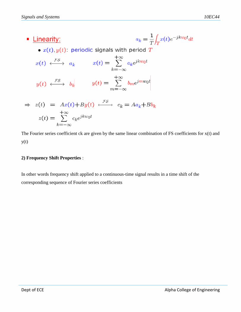
1) Linearity Properties
Signals and Systems 10EC44
Dept of ECE Alpha College of Engineering
The Fourier series coefficient ck are given by the same linear combination of FS coefficients for x(t) and
y(t)
2) Frequency Shift Properties :
In other words frequency shift applied to a continuous-time signal results in a time shift of the
corresponding sequence of Fourier series coefficients

Signals and Systems 10EC44
Dept of ECE Alpha College of Engineering
3) Scaling Properties :
4) Time Differentiation

Signals and Systems 10EC44
Dept of ECE Alpha College of Engineering
5) Modulation or Multiplication theorem

Signals and Systems 10EC44
Dept of ECE Alpha College of Engineering
Signals and Systems 10EC44
Dept of ECE Alpha College of Engineering
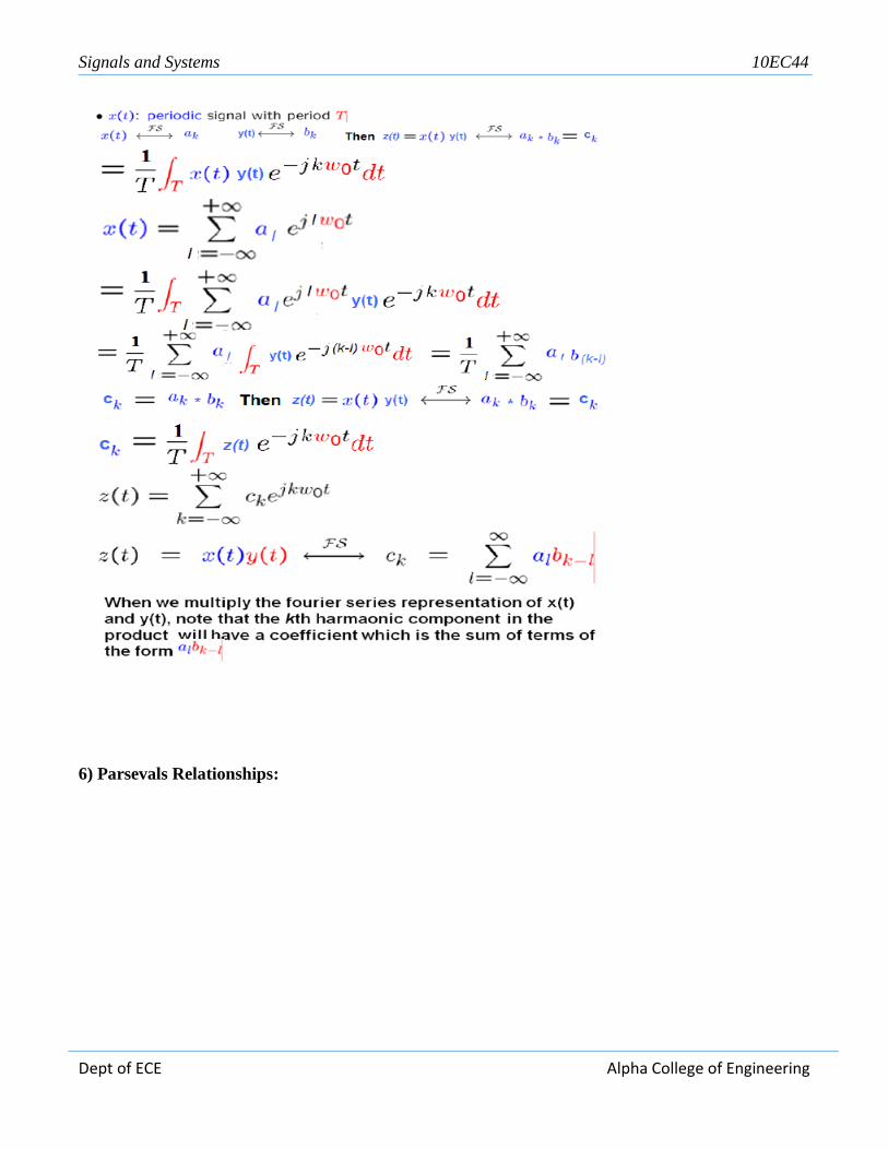
6) Parsevals Relationships:

Signals and Systems 10EC44
Dept of ECE Alpha College of Engineering

Signals and Systems 10EC44
Dept of ECE Alpha College of Engineering
Fourier Representation for Continuous Time Signals
Introduction Fourier Representation for Continuous Time Vs Discrete Time Signals
Some Important Differences

Signals and Systems 10EC44
Dept of ECE Alpha College of Engineering
• DTFS is a finite series while FS is an infinite series representation. Hence mathematical convergence
issues are not there in DTFS.
• Discrete-time signal x[n] is periodic with period N. i.ex[n] = x[n+N]
• The fundamental period is the smallest positive integer N for which the above holds and ωo= 2π/N and
φk[n] = ejkωon= ejk(2π/N)n , k = 0, ±1, ±2,…. Etc.
Discrete time Fourier Series
These Equations play the same role for discrete time periodic signals as the Synthesis and Analysis
Equations for Continuous time signals. akare referred to as the spectral coefficient of x[n]. These

Signals and Systems 10EC44
Dept of ECE Alpha College of Engineering
coefficients specify a decomposition of x[n] into a sum of N harmonically related complex exponentials.
We also observe that the graph nature both in Time domain and frequency domain are both discrete unlike
in Fourier Series for continuous times

Signals and Systems 10EC44
Dept of ECE Alpha College of Engineering
Unit 5
Fourier Representation for Signals
Learning Objectives:Fourier representation for signals – 2: Discrete and continuous Fourier
transforms(derivations of transforms are excluded) and their properties.
Discrete-Time Fourier Transform (DTFT)
Discrete-Time Fourier Transform
Inverse Discrete-Time Fourier Transform
Discrete-Time Fourier Transform Pair
When we obtain the discrete-time signal via sampling an analog signal, the Nyquist frequency corresponds
to the discrete-time frequency 1/2 . To show this, note that a sinusoid atthe Nyquist frequency 1/2Tshas a
sampled waveform that equalsSinusoid at Nyquist Freqency 1/2T
The exponential in the DTFT at frequency 1/2 equals
meaning that the correspondence between analog and discrete-time frequency is established:

Signals and Systems 10EC44
Dept of ECE Alpha College of Engineering
Analog, Discrete-Time Frequency Relationship
Where fD and fA represent discrete-time and analog frequency variables, respectively. The aliasing figure
(pg??) provides another way of deriving this result. As the duration of each pulse in the periodic sampling
signal pTs(t) narrows, the amplitudes of the signal’s spectral repetitions, which are governed by the
Fourier series coefficients (pg??) of pTs(t) , become increasingly equal.Thus, the sampled signal’s
spectrum becomes periodic with period1/ Ts Thus, the Nyquist frequency 1/2Ts orresponds to the
frequency 1/2 . The inverse discrete-time Fourier transform is easily derived from the following
relationship:
Figure:Discrete-Time Fourier Transform Properties
Therefore, we find that
Signals and Systems 10EC44
Dept of ECE Alpha College of Engineering
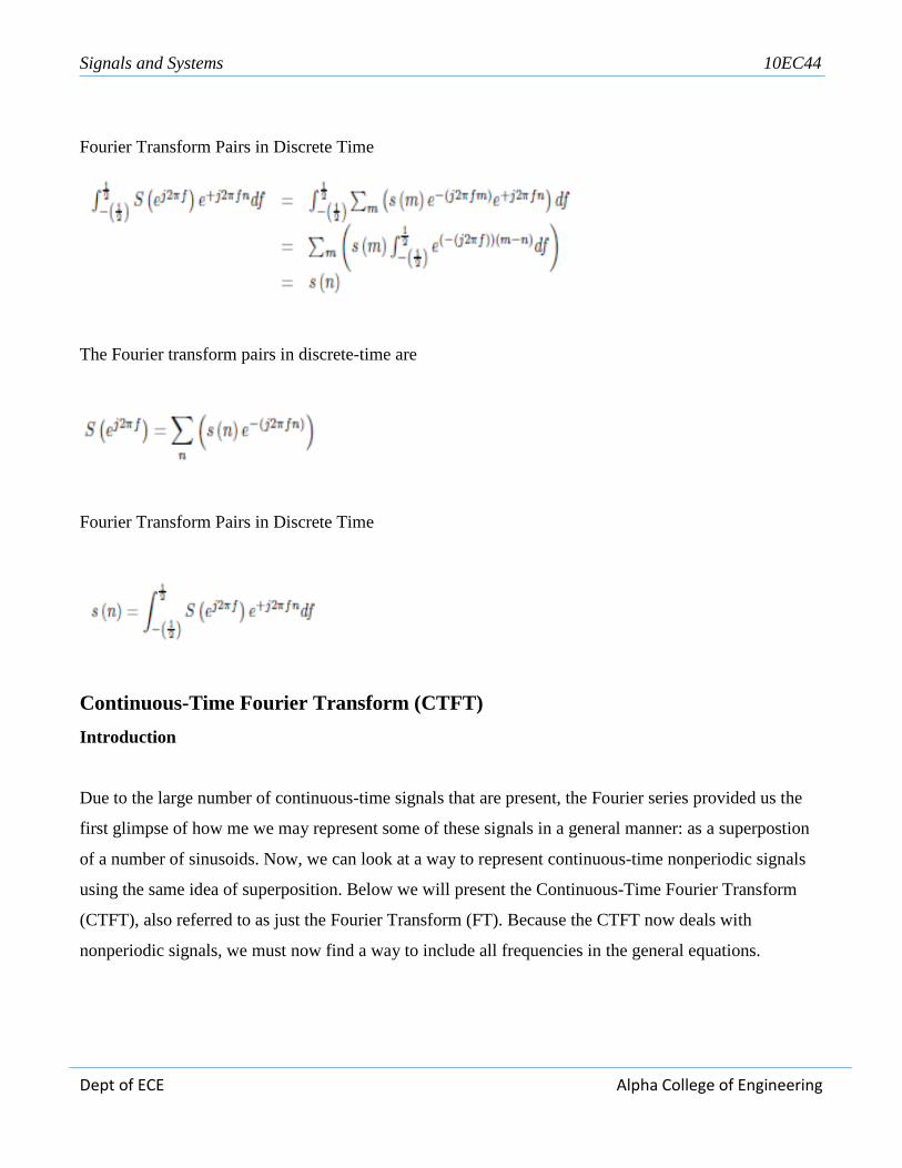
Fourier Transform Pairs in Discrete Time
The Fourier transform pairs in discrete-time are
Fourier Transform Pairs in Discrete Time
Continuous-Time Fourier Transform (CTFT)
Introduction
Due to the large number of continuous-time signals that are present, the Fourier series provided us the
first glimpse of how me we may represent some of these signals in a general manner: as a superpostion
of a number of sinusoids. Now, we can look at a way to represent continuous-time nonperiodic signals
using the same idea of superposition. Below we will present the Continuous-Time Fourier Transform
(CTFT), also referred to as just the Fourier Transform (FT). Because the CTFT now deals with
nonperiodic signals, we must now find a way to include all frequencies in the general equations.

Signals and Systems 10EC44
Dept of ECE Alpha College of Engineering
Figure: The spectrum of a length-ten pulse is shown. Can you explain the rather
complicated appearance of the phase?
Equations
Continuous-Time Fourier Transform
Inverse CTFT
Signals and Systems 10EC44
Dept of ECE Alpha College of Engineering
The above equations for the CTFT and its inverse come directly from the Fourier series and our
understanding of its coefficients. For the CTFT we simply utilize integration rather than summation to be
able to express the aperiodic signals. This should make sense since for the CTFT we are simply extending
the ideas of the Fourier series to include nonperiodic signals, and thus the entire frequency spectrum. Look
at the Derivation of the Fourier Transform for a more in depth look at this.
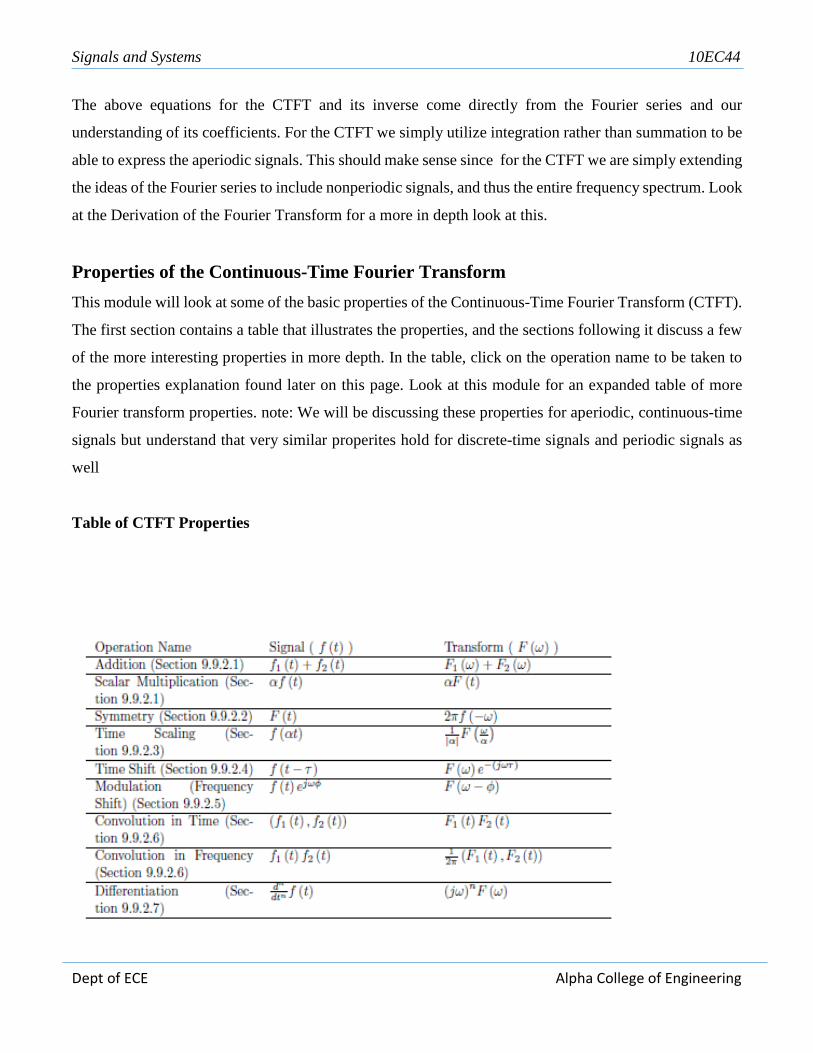
Properties of the Continuous-Time Fourier Transform
This module will look at some of the basic properties of the Continuous-Time Fourier Transform (CTFT).
The first section contains a table that illustrates the properties, and the sections following it discuss a few
of the more interesting properties in more depth. In the table, click on the operation name to be taken to
the properties explanation found later on this page. Look at this module for an expanded table of more
Fourier transform properties. note: We will be discussing these properties for aperiodic, continuous-time
signals but understand that very similar properites hold for discrete-time signals and periodic signals as
well
Table of CTFT Properties

Signals and Systems 10EC44
Dept of ECE Alpha College of Engineering
Fourier Transform Properties
Linearity
The combined addition and scalar multiplication properties in the table above demonstrate the basic
property of linearity. What you should see is that if one takes the Fourier transform of a linear combination
of signals then it will be the same as the linear combination of the Fourier transforms of each of the
individual signals. This is crucial when using a table of transforms to find the transform of a more
complicated signal.
We will begin with the following signal:
Now, after we take the Fourier transform, shown in the equation below, notice that
the linear combination of the terms is unaffected by the transform.
Symmetry
Symmetry is a property that can make life quite easy when solving problems involving Fourier transforms.
Basically what this property says is that since a rectangular function in time is a sinc function in frequency,
then a sincfucntion in time will be a rectangular function in frequency. This is a direct result of the
similarity between the forward CTFT and the inverse CTFT. The only difference is the scaling by 2_ and
a frequency reversal.
Time Scaling
This property deals with the effect on the frequency-domain representation of a signal if the time variable
is altered. The most important concept to understand for the time scaling property is that signals that are
narrow in time will be broad in frequency and vice versa. The simplest example of this is a delta function,
a unit pulse (pg??) with a very small duration, in time that becomes an infinite-length constant function in
frequency. The table above shows this idea for the general transformation from the time-domain to the
frequency-domain of a signal. You should be able to easily notice that these equations show the
relationship mentioned previously: if the time variable is increased then the frequency range will be
decreased.

Signals and Systems 10EC44
Dept of ECE Alpha College of Engineering
Time Shifting
Time shifting shows that a shift in time is equivalent to a linear phase shift in frequency. Since the
frequency content depends only on the shape of a signal, which is unchanged in a time shift, then only the
phase spectrum will be altered. This property can be easily proved using the Fourier Transform, so we
will show the basic steps below:
We will begin by letting z (t) = f (t −). Now let us take the Fourier transform
with the previous expression substitued in for z (t).
Now let us make a simple change of variables, where _ = t −_ . Through the calculations below, you
can see that only the variable in the exponential are altered thus only changing the phase in the
frequency domain.
Modulation (Frequency Shift)
Modulation is absolutely imperative to communications applications. Being able to shift a signal to a
different frequency, allows us to take advantage of different parts of the electromagnetic spectrum is what
allows us to transmit television, radio and other applications through the same space without significant
interference. The proof of the frequency shift property is very similar to that of the time shift however,
here we would use the inverse Fourier transform in place of the Fourier transform. Since we went through
the steps in the previous, time-shift proof, below we will just show the initial and final step to this proof:
Now we would simply reduce this equation through another change of variables and simplify
the terms. Then we will prove the property experssed in the table above

Signals and Systems 10EC44
Dept of ECE Alpha College of Engineering
Convolution
Convolution is one of the big reasons for converting signals to the frequency domain, since convolution
in time becomes multiplication in frequency. This property is also another excellent example of symmetry
between time and frequency. It also shows that there may be little to gain by changing to the frequency
domain when multiplication in time is involved. We will introduce the convolution integral here, but if
you have not seen this before or need to refresh your memory, then look at the continuous-time
convolution module for a more in depth explanation and derivation
Time Differentiation
Since LTI systems can be represented in terms of differential equations, it is apparent with this property
that converting to the frequency domain may allow us to convert these complicated
differential equations to simpler equations involving multiplication and addition. This is often looked at
in more detail during the study of the Laplace Transform.

Signals and Systems 10EC44
Dept of ECE Alpha College of Engineering
Unit 6
Applications Of Fourier Representations
Learning Objectives:Applications of Fourier representations: Introduction, Frequency
response of LTI systems, Fourier transform representation of periodic signals, Fourier transform
representation of discrete time signals. Sampling theorm and Nyquist rate.

Signals and Systems 10EC44
Dept of ECE Alpha College of Engineering
FT FOR PERIODIC SIGNALS: For analysing Discrete time periodic and a periodic signals DTFT is
used. As in continuous time case, DT periodic signals can be incorporated within the framework of the
DTFT, by interpreting the transform of periodic signal as an impulse train in the frequency domain
• Fourier Transform from Fourier series

Signals and Systems 10EC44
Dept of ECE Alpha College of Engineering
Fourier Transform from Fourier series In order to check the validity of the above expression let us
use the synthesys equation.
Fourier Transform from Fourier series Note that any interval of length 2π includes exactly one pulse
in the above analysis eqn. Hence if the integral interval is chosen includes one pulse located at ωo+2πr,
then
Now consider a periodic sequence x[n] with period N its DTFS representation is

Signals and Systems 10EC44
Dept of ECE Alpha College of Engineering
So that the FS can be directly constructed from
its coefficient. To verify the above equation is correct note that x[n] in the above is a linear combination
of and thus must be a combination of transforms
In this case, the Fourier transform is
So that the FS can be directly constructed from its coefficient. To verify the above equation is correct
note that x[n] in the above is a linear combination of and thus must be a combination of transforms
Fourier Transform from Fourier series
Suppose we chose the summation of interval as k=0,1……N, so that
Hence x[n] is a linear combination of signals as initial x[n]. With ω0 =0,2π/N, 4π/N,……. (N-1)2π/N.
The waveforms are depicted as

Signals and Systems 10EC44
Dept of ECE Alpha College of Engineering

Signals and Systems 10EC44
Dept of ECE Alpha College of Engineering

Signals and Systems 10EC44
Dept of ECE Alpha College of Engineering

Signals and Systems 10EC44
Dept of ECE Alpha College of Engineering
Example 1

Signals and Systems 10EC44
Dept of ECE Alpha College of Engineering

Signals and Systems 10EC44
Dept of ECE Alpha College of Engineering

Signals and Systems 10EC44
Dept of ECE Alpha College of Engineering

Signals and Systems 10EC44
Dept of ECE Alpha College of Engineering

Signals and Systems 10EC44
Dept of ECE Alpha College of Engineering
Summaries Fourier in LTI
• The LTI system scales the complex exponential eiωt.
• Each system has its own constant H(ω) that describes how it scales eigenfunctions. It is called the
frequency response.
• The frequency response H(ω) does not depend on the input. It is another way to describe a system, like
(A, B, C, D), h, etc.
• If we know H(ω), it is easy to find the output when the input is an eigenfunction. y(t)=H(ω)x(t) true
when x is eigenfunction!
Differential and Difference Equation Descriptions Frequency Response is the system‟s steady state
response to a sinusoid. In contrast to differential and difference-equation descriptions for a system, the
frequency response description cannot represent initial conditions, it can only describe a system in a
steady state condition. The differential-equation representation for a continuous-time system is

Signals and Systems 10EC44
Dept of ECE Alpha College of Engineering

Signals and Systems 10EC44
Dept of ECE Alpha College of Engineering

Signals and Systems 10EC44
Dept of ECE Alpha College of Engineering

Signals and Systems 10EC44
Dept of ECE Alpha College of Engineering

Signals and Systems 10EC44
Dept of ECE Alpha College of Engineering

Signals and Systems 10EC44
Dept of ECE Alpha College of Engineering

Signals and Systems 10EC44
Dept of ECE Alpha College of Engineering
Sampling
In this chapter let us understand the meaning of sampling and which are the different methods of
sampling. There are the two types. Sampling Continuous-time signals and Sub-sampling. In this again
we have Sampling Discrete-time signals. Sampling Continuous-time signals Sampling of continuous-
time signals is performed to process the signal using digital processors. The sampling operation
generates a discrete-time signal from a continuous-time signal.DTFT is used to analyze the effects of
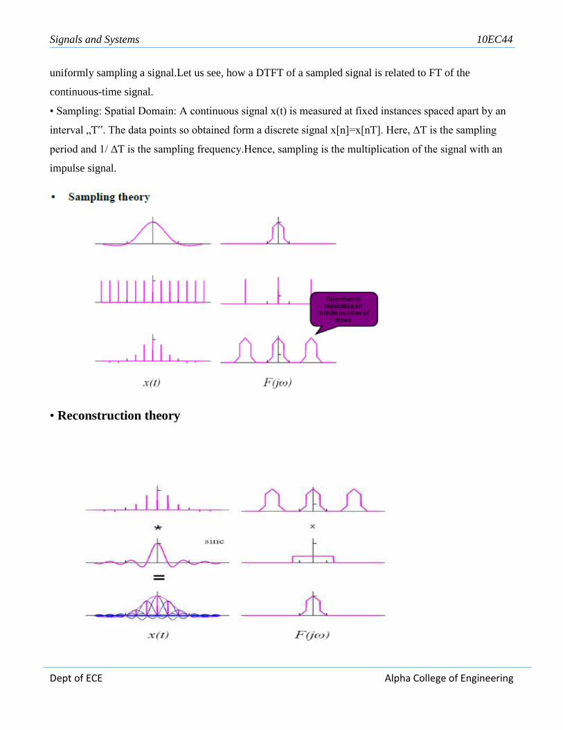
Signals and Systems 10EC44
Dept of ECE Alpha College of Engineering
uniformly sampling a signal.Let us see, how a DTFT of a sampled signal is related to FT of the
continuous-time signal.
• Sampling: Spatial Domain: A continuous signal x(t) is measured at fixed instances spaced apart by an
interval „Ƭ‟. The data points so obtained form a discrete signal x[n]=x[nƬ]. Here, ΔƬ is the sampling
period and 1/ ΔƬ is the sampling frequency.Hence, sampling is the multiplication of the signal with an
impulse signal.
• Reconstruction theory

Signals and Systems 10EC44
Dept of ECE Alpha College of Engineering

Signals and Systems 10EC44
Dept of ECE Alpha College of Engineering

Signals and Systems 10EC44
Dept of ECE Alpha College of Engineering

Signals and Systems 10EC44
Dept of ECE Alpha College of Engineering
Sampling below the Nyquist rate
Reconstruction below the Nyquist rate

Signals and Systems 10EC44
Dept of ECE Alpha College of Engineering
Aliasing summary
• We learned that we need to sample each oscillation period of the input signal ≥ two times for good
reconstruction.(Nyquist Criteria)
• The shifted version of X(jω) may overlap with each other if ωs(sampling frequency) is not large
enough compared to the frequency content of X(jω).
• Overlap in the shifted replicas of the original spectrum is termed Aliasing, which refers to the
phenomenon of a high frequency component taking on the identity of a low-frequency one.
FT of sampled signal for different sampling frequency

Signals and Systems 10EC44
Dept of ECE Alpha College of Engineering
Subsampling: Sampling discrete-time signal
• FT is also used in discrete sampling signal.
• Let be a subsampled version x[n], where q is a positive integer.
• Relating DTFT of y[n] to the DTFT of x[n], by using FT to represent x[n] as a sampled versioned of a
continuous time signal x(t).
• Expressing now y[n] as a sampled version of the sampled version of the same underlying CT x(t)
obtained using a sampling interval q that associated with x[n]
• We know to represent the sampling version of x[n] as the impulse sampled CT signal with sampling
interval Ƭ.

Signals and Systems 10EC44
Dept of ECE Alpha College of Engineering

Signals and Systems 10EC44
Dept of ECE Alpha College of Engineering
UNIT 7
Z TRANSFORMS-1
Learning Objectives:Introduction, Z – transform, properties of ROC, Properties of Z –
transforms, inversion of Z – transforms.
Introduction
The z-transform is a transform for sequences. Just like the Laplace transformtakes a function of t and
replaces it with another function of an auxiliaryvariable s. The z-transform takes a sequence and replaces
it with afunction of an auxiliary variable, z. The reason for doing this is that itmakes difference equations
easier to solve, again, this is very like what happenswith the Laplace transform, where taking the Laplace
transform makesit easier to solve differential equations. A difference equation is an equationwhich tells
you what the k+2th term in a sequence is in terms of the k+1thand kth terms, for example. Difference
equations arise in numerical treatmentsof differential equations, in discrete time sampling and when
studyingsystems that are intrinsically discrete, such as population models in ecologyand epidemiology
and mathematical modelling of mylinated nerves.
Generalizes the complex sinusoidal representations of DTFT to more generalized representation
using complex exponential signals
It is the discrete time counterpart of Laplace transform

Signals and Systems 10EC44
Dept of ECE Alpha College of Engineering
The z-Plane
•Complex number z = re jis represented as a location in a complex plane (z plane)
The z-transform
• Let z = re j be a complex number with magnitude r and angle .
• The signal x[n] = znis a complex exponential and x[n] = rncos(n)+jrnsin(n)
• The real part of x[n] is exponentially damped cosine.
• The imaginary part of x[n] is exponentially damped sine.
• Apply x[n] to an LTI system with impulse response h[n], Then
y[n] = H{x[n]} = h[n] ∗x[n]

Signals and Systems 10EC44
Dept of ECE Alpha College of Engineering
y[n] =∑ ℎ[𝑘]𝑥[𝑛 − 𝑘]∞𝑘=−∞
•If x[n] = zn
we get
The z-transform is defined as
we may write as
You can see that when you do the z-transformit sums up all the sequence, and so the individual terms
affect the dependence on z, but the resultingfunction is just a function of z, it has no k in it. It will become
clearer later why we might do this

Signals and Systems 10EC44
Dept of ECE Alpha College of Engineering
•This has the form of an eigen relation, where znis the eigen function and H(z) is the eigenvalue.
•The action of an LTI system is equivalent to multiplication of the input by the complex number H(z).
•IfH(z) = |H(z)|e j(z)then the system output is
y[n] = |H(z)|e j(z)zn
•Usingz = re jwe get
y[n] = |H(re j)|rncos(n+(re j)+ j|H(re j)|rnsin(n+(re j)
•Rewritingx[n]
x[n] = zn= rncos(n)+ jrnsin(n)
•If we compare x[n] and y[n], we see that the system modifies
– the amplitude of the input by|H(re j)| and
– shifts the phase by (re j)
DTFT and the z-transform
•Put the value of z in the transform then we get

Signals and Systems 10EC44
Dept of ECE Alpha College of Engineering
•We see that H(re j) corresponds to DTFT of h[n]r−n.
•The inverse DTFT of H(re j) must be h[n]r−n.
•We can write
•Multiplying h[n]r−nwith rngives
•We can convert this equation into an integral over z by putting re j=z
•Integration is over , we may consider r as a constant
•We have

Signals and Systems 10EC44
Dept of ECE Alpha College of Engineering
•Consider limits on integral
– varies from −to
– ztraverses a circle of radius r in a counterclockwise direction
We can write h[n] as
where H is integration around the circle of radius |z| = r in a counter clockwise direction
• The z-transform of any signal x[n] is
• The inverse z-transform of is
• Inverse z-transform expresses x[n] as a weighted superposition of complex exponentialsZn
• The weights are
• This requires the knowledge of complex variable theory.
Convergence
• Existence of z-transform: exists only if
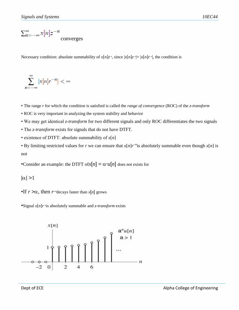
Signals and Systems 10EC44
Dept of ECE Alpha College of Engineering
converges
Necessary condition: absolute summability of x[n]z−n, since |x[n]z−n|= |x[n]r−n|, the condition is
• The range r for which the condition is satisfied is called the range of convergence (ROC) of the z-transform
• ROC is very important in analyzing the system stability and behavior
• We may get identical z-transform for two different signals and only ROC differentiates the two signals
• The z-transform exists for signals that do not have DTFT.
• existence of DTFT: absolute summability of x[n]
• By limiting restricted values for r we can ensure that x[n]r−nis absolutely summable even though x[n] is
not
•Consider an example: the DTFT ofx[n] = nu[n] does not exists for
|| >1
•If r >, then r−ndecays faster than x[n] grows
•Signal x[n]r−nis absolutely summable and z-transform exists
Signals and Systems 10EC44
Dept of ECE Alpha College of Engineering
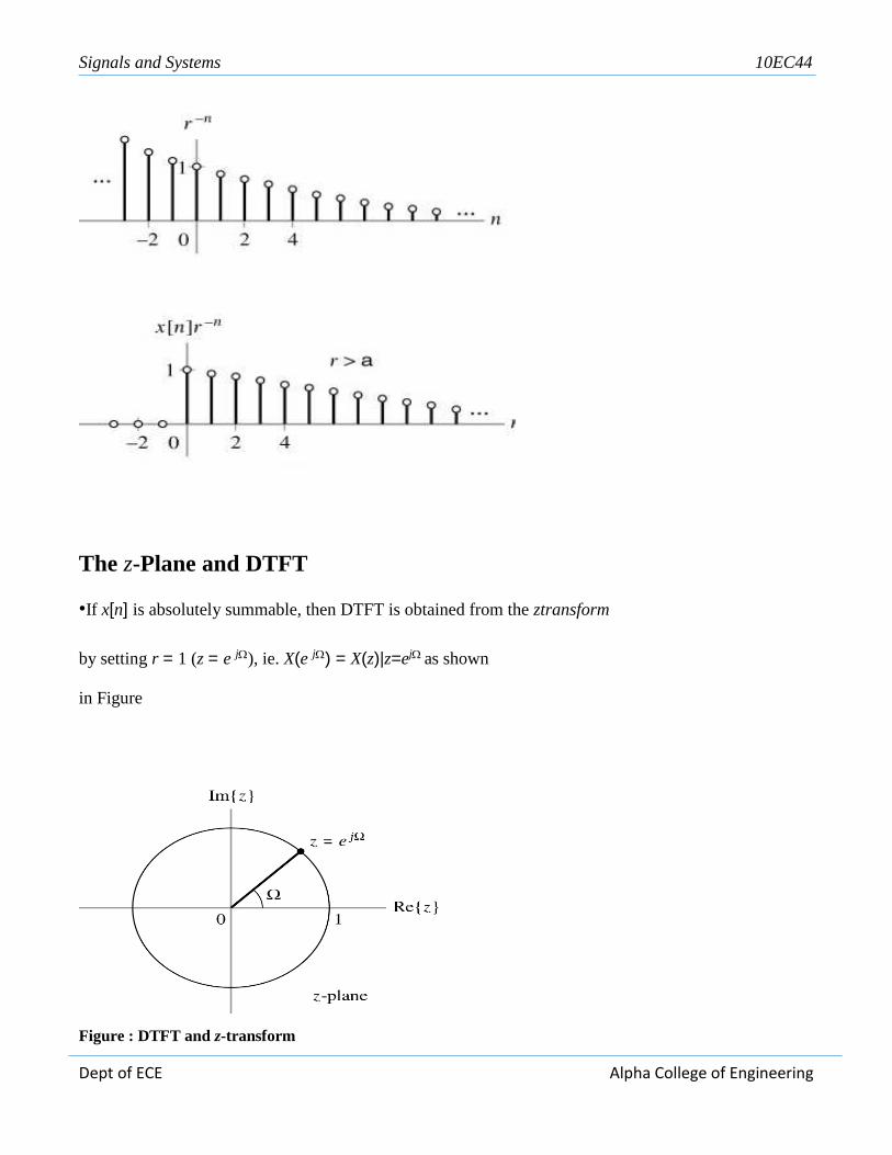
The z-Plane and DTFT
•If x[n] is absolutely summable, then DTFT is obtained from the ztransform
by setting r = 1 (z = e j), ie. X(e j) = X(z)|z=ejas shown
in Figure
Figure : DTFT and z-transform
Signals and Systems 10EC44
Dept of ECE Alpha College of Engineering
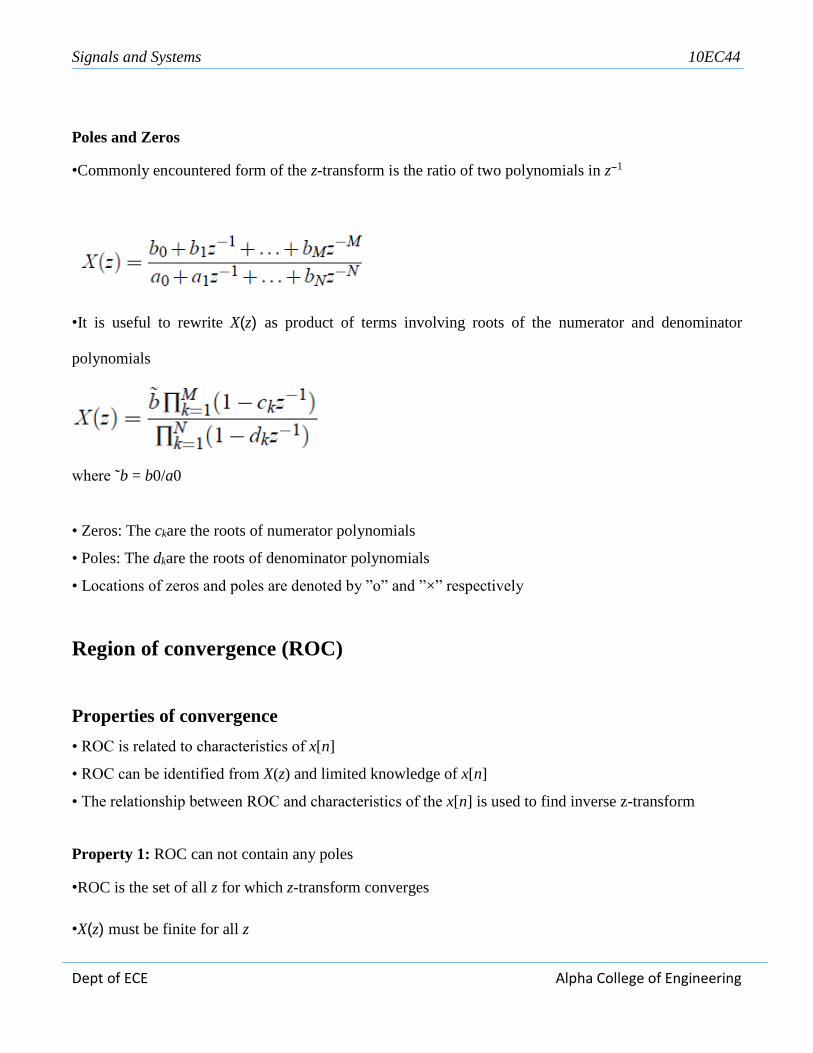
Poles and Zeros
•Commonly encountered form of the z-transform is the ratio of two polynomials in z−1
•It is useful to rewrite X(z) as product of terms involving roots of the numerator and denominator
polynomials
where ˜b = b0/a0
• Zeros: The ckare the roots of numerator polynomials
• Poles: The dkare the roots of denominator polynomials
• Locations of zeros and poles are denoted by ”o” and ”×” respectively
Region of convergence (ROC)
Properties of convergence
• ROC is related to characteristics of x[n]
• ROC can be identified from X(z) and limited knowledge of x[n]
• The relationship between ROC and characteristics of the x[n] is used to find inverse z-transform
Property 1: ROC can not contain any poles
•ROC is the set of all z for which z-transform converges
•X(z) must be finite for all z

Signals and Systems 10EC44
Dept of ECE Alpha College of Engineering
•If p is a pole, then |H(p)| = and z-transform does not converge at
the pole
•Pole can not lie in the ROC
Property 2: The ROC for a finite duration signal includes entire z-plane except z = 0
or/and z =
•Let x[n] be nonzero on the interval n1 ≤n ≤n2. The z-transform is
The ROC for a finite duration signal includes entire z-plane except z = 0 or/and z =
•If a signal is causal (n2 >0) then X(z) will have a term containing z−1, hence ROC can not include z = 0
•If a signal is non-causal (n1 <0) then X(z) will have a term containing powers of z, hence ROC can not
include z = The ROC for a finite duration signal includes entire z-plane except z = 0 or/and z =
•If n2 ≤0 then the ROC will include z = 0If n1 ≥0 then the ROC will include z =
•This shows the only signal whose ROC is entire z-plane is x[n] = c[n],where c is a constant
Finite duration signals
•The condition for convergence is |X(z)| <
magnitude of sum of complex numbers ≤sum of individual magnitudes

Signals and Systems 10EC44
Dept of ECE Alpha College of Engineering
•Magnitude of the product is equal to product of the magnitudes
•split the sum into negative and positive time parts
•Let
• Note that X(z) = I−(z)+I+(z). If both I−(z) and I+(z) are finite, then X(z) if finite
• If x[n] is bounded for smallest +ve constants A−, A+, r− and r+such That
|x[n]| ≤A−(r−)n, n <0
|x[n]| ≤A+(r+)n, n ≥0
•The signal that satisfies above two bounds grows no faster than (r+)nfor +ve n and (r−)nfor −ve n
•If the n <0 bound is satisfied then
• Sum converges if |z| ≤ r−
• If the n ≥ 0 bound is satisfied then

Signals and Systems 10EC44
Dept of ECE Alpha College of Engineering
• Sum converges if |z| >r+
• If r+<|z|<r−, then both I+(z) and I−(z) converge and X(z) converges
To summarize:
• If r+ >r− then no value of z for which convergence is guaranteed
• Left handed signal is one for which x[n] = 0 for n ≥ 0
• Right handed signal is one for which x[n] = 0 for n < 0
• Two sided signal that has infinite duration in both +ve and -ve directions
• The ROC of a right-sided signal is of the form |z| >r+
• The ROC of a left-sided signal is of the form |z| <r−
• The ROC of a two-sided signal is of the form r+ <|z| >r−
Figure : ROC of left sided sequence

Signals and Systems 10EC44
Dept of ECE Alpha College of Engineering
Figure: ROC of right sided sequence
Figure: ROC of two sided sequence
Figure : ROC of Example 1

Signals and Systems 10EC44
Dept of ECE Alpha College of Engineering
Properties of z-transform
•We assume that
• General form of the ROC is a ring in the z-plane, so the effect of an operation on the ROC is described
by the a change in the radii of ROC
P1: Linearity
•The z-transformof a sum of signals is the sumof individual z-transforms
with ROC at least Rx ∩Ry
P2: Time reversal
• Time reversal or reflection corresponds to replacing z by z−1. Hence, if Rx is of the form a <|z| <b then
the ROC of the reflected signal is a < 1/|z| <b or 1/b <|z| < 1/a
If
with ROC Rx
Then
with ROC 1/Rx

Signals and Systems 10EC44
Dept of ECE Alpha College of Engineering
Proof: Time reversal
•Let
Let l = −n, then
P3: Time shift
•Time shift of no in the time domain corresponds to multiplication of z−noin the z-domain
If
with ROC Rx
Then
with ROC Rx except z = 0 or |z| =
Time shift, no >0
•Multiplication by z−nointroduces a pole of order no at z = 0
•The ROC can not include z = 0, even if Rx does include z = 0

Signals and Systems 10EC44
Dept of ECE Alpha College of Engineering
•If X(z) has a zero of at least order no at z = 0 that cancels all of the new poles then ROC can include z =
0
Time shift, no <0
•Multiplication by z−no introduces no poles at infinity
•If these poles are not canceled by zeros at infinity in X(z) then the ROC of z−noX(z) can not include |z| =
Proof: Time shift
•Let
P4: Multiplication by n
•Let be a complex number
If
with ROC Rx
Then

Signals and Systems 10EC44
Dept of ECE Alpha College of Engineering
with ROC ||Rx
• ||Rx indicates that the ROC boundaries are multiplied by ||.
•If Rx is a <|z| <b then the new ROC is ||a <|z| <||b
•If X(z) contains a pole d, ie. the factor (z−d) is in the denominator then X(z) has a factor (z−d) in the
denominator and thus a pole atd.
•If X(z) contains a zero c, then X(z/) has a zero at c
•This indicates that the poles and zeros of X(z) have their radii changed by ||
•Their angles are changed by arg{}
•If || =1 then the radius is unchanged and if is +ve real number then the angle is unchanged
Proof: Multiplication by n
•Let y[n] = nx[n]

Signals and Systems 10EC44
Dept of ECE Alpha College of Engineering
P5: Convolution
•Convolution in time domain corresponds to multiplication in the zdomain
If
with ROC Rx
with ROC Ry
with ROC at least Rx ∩Ry
•Similar to linearity the ROC may be larger than the intersection of Rx
andRy
Proof: Convolution
•Let

Signals and Systems 10EC44
Dept of ECE Alpha College of Engineering
P6: Differentiation in the z domain
•Multiplication by n in the time domain corresponds to differentiation with respect to z and multiplication
of the result by −z in the z-domain.
If
with ROC Rx Then
with ROC Rx
•ROC remains unchanged
Proof: Differentiation in the z domain
•We know

Signals and Systems 10EC44
Dept of ECE Alpha College of Engineering
Differentiate with respect to z
• Multiply with −z
Then
with ROC Rx
Inverse z-transform
Partial fraction method
•In case of LTI systems, commonly encountered form of z-transform is
Usually M <N

Signals and Systems 10EC44
Dept of ECE Alpha College of Engineering
•If M >N then use long division method and express X(z) in the form
where ˜B(z) now has the order one less than the denominator polynomial and use partial fraction method
to find z-transform
•The inverse z-transform of the terms in the summation are obtained from the transform pair and time shift
property
•If X(z) is expressed as ratio of polynomials in z instead of z−1 then convert into the polynomial of z−1
•Convert the denominator into product of first-order terms
wheredkare the poles of X(z)
For distinct poles
•For all distinct poles, the X(z) can be written as

Signals and Systems 10EC44
Dept of ECE Alpha College of Engineering
•Depending on ROC, the inverse z-transform associated with each term is then determined by using the
appropriate transform pair
•We get
with ROC z >dkOR
with ROC z <dk
•For each term the relationship between the ROC associated with X(z) and each pole determines whether
the right-sided or left sided inversetransform is selected
For Repeated poles
•If pole di is repeated r times, then there are r terms in the partial fraction expansion associated with that
pole
•Here also, the ROC of X(z) determines whether the right or left sided inverse transform is chosen
withROC|z|>di
•If the ROC is of the form |z| <di, the left-sided inverse z-transform is chosen, ie

Signals and Systems 10EC44
Dept of ECE Alpha College of Engineering
Deciding ROC
•The ROC of X(z) is the intersection of the ROCs associated with the individual terms in the partial fraction
expansion.
•In order to chose the correct inverse z-transform, we must infer the ROC of each term from the ROC of
X(z).
•By comparing the location of each pole with the ROC of X(z).
•Chose the right sided inverse transform: if the ROC of X(z) has the radius greater than that of the pole
associated with the given term
•Chose the left sided inverse transform: if the ROC of X(z) has the radius less than that of the pole
associated with the given term
Power series expansion
•Express X(z) as a power series in z−1 or z as given in z-transform equation
•The values of the signal x[n] are then given by coefficient associated with z−n
•Main disadvantage: limited to one sided signals
•Signals with ROCs of the form |z| >a or |z| <a
•If the ROC is |z| >a, then express X(z) as a power series in z−1and we get right sided signal
•If the ROC is |z| <a, then express X(z) as a power series in z and we get left sided signal.

Signals and Systems 10EC44
Dept of ECE Alpha College of Engineering
UNIT 8
Z TRANSFORMS-2
Learning Objectives:Transform analysis of LTI Systems, unilateral Z Transform and its
application to solve difference equations
The Transfer Function
•We have defined the transfer function as the z-transform of the impulse response of an LTI system
•Then we have y[n] = x[n] ∗h[n] and Y(z) = X(z)H(z)
•This is another method of representing the system
•The transfer function can be written as
•This is true for all z in the ROCs of X(z) and Y(z) for which X(z) in nonzero
•The impulse response is the z-transform of the transfer function
•We need to know ROC in order to uniquely find the impulse response
•If ROC is unknown, then we must know other characteristics such as stability or causality in order to
uniquely find the impulse response
Relation between transfer function and difference equation

Signals and Systems 10EC44
Dept of ECE Alpha College of Engineering
• The transfer can be obtained directly from the difference-equation description of an LTI system
• We know that
• We know that the transfer function H(z) is an eigen value of the system associated with the eigen function
zn, ie. ifx[n] = znthen the output of an LTI system y[n] = znH(z)
• Put x[n−k] = zn−k and y[n−k] = zn−k H(z) in the difference equation,
we get
• We can solve for H(z)
• The transfer function described by a difference equation is a ratio of polynomials in z−1 and is termed as
a rational transfer function.
• The coefficient of z−kin the numerator polynomial is the coefficient associated with x[n−k] in the
difference equation
• The coefficient of z−kin the denominator polynomial is the coefficient associated with y[n−k] in the
difference equation
• This relation allows us to find the transfer function and also find thedifference equation description for
a system, given a rational function
Transfer function
• The poles and zeros of a rational function offer much insight into LTI system characteristics
• The transfer function can be expressed in pole-zero form by factoring the numerator and denominator
polynomial

Signals and Systems 10EC44
Dept of ECE Alpha College of Engineering
• If ckand dkare zeros and poles of the system respectively and ˜b = b0/a0 is the gain factor, then
• This form assumes there are no poles and zeros at z = 0
• The pthorder pole at z = 0 occurs when b0 = b1 = . . . = bp−1 = 0
• The lth order zero at z = 0 occurs when a0 = a1 = . . . = al−1 = 0
• Then we can write H(z) as
where ˜b = bp/al
• In the example we had first order pole at z = 0
• The poles, zeros and gain factor˜buniquely determine the transfer function
• This is another description for input-output behavior of the system
• The poles are the roots of characteristic equation
Causality, stability and Inverse systems
Causality
• The impulse response of an LTI system is zero for n < 0
• The impulse response of a causal LTI system is determined from the transfer function by using right
sided inverse transforms
• The pole inside the unit circle in the z-plane contributes an exponentially decaying term
• The pole outside the unit circle in the z-plane contributes an exponentially increasing term

Signals and Systems 10EC44
Dept of ECE Alpha College of Engineering
Stability
• The system is stable: if impulse response is absolutely summable and DTFT of impulse response exists
• The ROC must include the unit circle: the pole and unit circle together define the behavior of the system
Figure: When the pole is inside the unit circle
Figure: When the pole is outside the unit circle

Signals and Systems 10EC44
Dept of ECE Alpha College of Engineering
Figure: Stability: When the pole is inside the unit circle
• A stable impulse response can not contain any increasing exponential term
• The pole inside the unit circle in the z-plane contributes right-sided exponentially decaying term
• The pole outside the unit circle in the z-plane contributes left-sided exponentially decaying term
Causal and stable system
• Stable and causal LTI system: all the poles must be inside the unit circle
• A inside pole contributes right sided or causal exponentially decaying system
• A outside pole contributes either left sided decaying term which is not causal or right-sided exponentially
increasing term which is not stable
Figure : Stability: When the pole is outside the unit circle

Signals and Systems 10EC44
Dept of ECE Alpha College of Engineering
Figure : Location of poles for the causal and stable system
• Example of stable and causal system: all the poles are inside the unit Circle
Inverse system
• Impulse response (hinv) of an inverse system satisfies hinv[n] ∗h[n] = [n] where h[n] is the impulse
response of a system to be inverted
• Take inverse z-transform on both sides gives
Hinv(z)H(z) = 1
Hinv(z) =1/H(z)
• The transfer function of an LTI inverse system is the inverse of thetransfer function of the system that
we desire to invert
• If we write the pole-zero form of H(z) as
where ˜b = bp/al
• Then we can write Hinvas

Signals and Systems 10EC44
Dept of ECE Alpha College of Engineering
• The zeros of H(z) are the poles of Hinv(z)
• The poles of H(z) are the zeros of Hinv(z)
• System defined by a rational transfer function has an inverse system
• We need inverse systems which are both stable and causal to invert the distortions introduced by the
system
• The inverse system Hinv(z) is stable and causal if all poles are inside the unit circle
• Poles of Hinv(z) are zeros of (z)
• Inverse system Hinv(z): stable and causal inverse of an LTI system H(z) exists if and only if all the zeros
of H(z) are inside the unit circle
• The system with all its poles and zeros inside the unit circle is called as minimum-phase system
• The magnitude response is uniquely determined by the phase response and vice-Vera
• For a minimum-phase system the magnitude response is uniquely determined by the phase response and
vice-versa
Figure: Location of poles in a minimum-phase system

Signals and Systems 10EC44
Dept of ECE Alpha College of Engineering
Unilateral z-transform
•Useful in case of causal signals and LTI systems
•The choice of time origin is arbitrary, so we may choose n = 0 as the time at which the input is applied
and then study the response for times n ≥0
Advantages
•We do not need to use ROCs
•It allows the study of LTI systems described by the difference equation with initial conditions
Unilateral z-transform
•The unilateral z-transform of a signal x[n] is defined as
which depends only on x[n] for n ≥0
•The unilateral and bilateral z-transforms are equivalent for causal signals
Properties
•The same properties are satisfied by both unilateral and bilateral ztransformswith one exception: the time
shift property

Signals and Systems 10EC44
Dept of ECE Alpha College of Engineering
•The time shift property for unilateral z-transform: Let w[n] = x[n−1]
•The unilateral z-transform of w[n] is
•The unilateral z-transform of w[n] is
•A one-unit time shift results in multiplication by z−1 and addition of
the constant x[−1]
•In a similar way, the time-shift property for delays greater than unity is

Signals and Systems 10EC44
Dept of ECE Alpha College of Engineering
•In the case of time advance, the time-shift property changes to

![Ece IV Signals & Systems [10ec44] Assignment](https://static.fdocuments.net/doc/165x107/55cf8f0c550346703b9866cd/ece-iv-signals-systems-10ec44-assignment.jpg)