Signaling and Productivity in the Private Financial

Returns to Schooling

Paul Bingley1, Kaare Christensen2, and Kristoffer Markwardt1

1SFI - The Danish National Centre for Social Research2The Danish Twin Registry, University of Southern Denmark

Abstract

Does formal schooling contribute to individual labor market productivity or doesit act as a signal to employers of predetermined labor market skills? Different em-pirical approaches have been proposed to answer this question. Using data fromadministrative registries on the population of Denmark, including detailed informa-tion on sibling type, we apply two of the prominent empirical strategies in the sameinstitutional setting and create a link between them. We further propose a novel testfor the existence of job market signaling and provide new evidence on the relativeimportance of signaling for the private financial returns to schooling. We find thatsignaling explains most (if not all) of the returns to schooling. However, a humancapital model with rapid skill depreciation could be part of the explanation as well.

Keywords: human capital, signaling, earnings, employer learning

JEL Classification: D8, I20, J31, J41

We are grateful to Mette Ejrnæs, Nabanita Datta Gupta, Thais Lærkholm Jensen, Søren Leth-Petersen,and Steve Machin for comments. Funding was provided by the Danish Strategic Research Council (grantsDSF-09-065167 and DSF-09-070295). All errors and omissions are our own. Corresponding authors: Bing-ley: pbingley@sfi.dk; Markwardt: ksm@sfi.dk

I. Introduction

A large body of empirical research has shown that individual investment in formal

schooling is associated with a subsequent wage premium. Although the size of the pre-

mium differs across countries, this conclusion holds across differently structured labor

markets with different institutions.

Less is known about what causes the wage premium. According to human capital

(HC) theory, schooling increases human capital which translates into increased indi-

vidual labor market productivity. Employers value the increased productivity and pay

wages accordingly. In contrast, the job market signaling (JMS) model assumes fixed pre-

determined individual labor market productivity. This information is private to workers,

who signal their abilities to potential employers through schooling attainment.

These competing explanations have substantially different implications for society.

Human capital accumulation at the individual level translates into productivity at the

firm level and thus growth at the aggregate level. In contrast, if skill sets are prede-

termined then formal training acquired in school acts merely as an ability signal to em-

ployers, who pay a premium for the schooling investment but do not enjoy a productivity

increase in exchange. Thus, in the JMS model schooling does not translate into produc-

tivity at the firm level and growth at the aggregate level. Therefore, JMS generates a

wedge between private and social returns to schooling.

In the literature different empirical strategies to disentangling the HC and JMS the-

ories have been applied. This paper creates a link between the two main estimation

strategies within the most prominent strand of the literature, often referred to as “em-

ployer learning”. Furthermore, this paper proposes a new test for the existence of JMS

and also presents new evidence on the relative importance of JMS for the private finan-

cial returns to schooling.

The employer learning strand of the literature exploits differences in assumptions

about the distribution of information in the JMS and HC models. In contrast to the HC

model, the JMS model assumes that employers are initially uncertain about workers’

productive types and therefore use schooling to predict individuals’ productivity. Em-

ployers then learn about workers’ productive types as time passes and workers gradually

2

reveal information about themselves through job performance.1

Some studies exploit presumed differences in the ease with which firms can learn

about individual productivity between different industries (Wolpin, 1977; Riley, 1979)

or types of job applicants (Albrecht, 1981). More recent contributions test for statisti-

cal discrimination and employer learning by assuming that the researcher can observe

a pre-market ability measure that is not observed by employers. This literature (Fos-

ter and Rosenzweig, 1993; Farber and Gibbons, 1996; Altonji and Pierret, 1997, 2001;

Galindo-Rueda, 2003; Lange and Topel, 2006; Lange, 2007 and others) evaluates how

the estimated returns to schooling and ability evolve over time.

Rather than including a pre-market ability measure, Miller, Mulvey, and Martin

(2004) compare returns to schooling differences of monozygotic (MZ) and dizygotic (DZ)

twins. Under the assumption that MZ twins are more productively alike than DZ twins,

employer learning implies that the the return to schooling differences for MZ twins de-

creases relative to DZ twins over time.

Our point of departure is the work by Altonji and Pierret (2001), who propose a test

for employer learning that relies on information which is initially unavailable to em-

ployers. Their work has served as a blueprint for later studies (Arcidiacono et al., 2010;

Bauer and Haisken-DeNew, 2001; Light and McGee, 2012; Mansour, 2012). Applying

this test to working-age males using data from administrative records on the Danish

population, we obtain results that are consistent with those of Altonji and Pierret (2001).

The data further allows us to run separate regressions by sibling type (non-twin, MZ,

and DZ), thereby enabling us to create a link from (Altonji and Pierret, 2001) to the twin

approach to employer learning. Having established this link, we apply the test based on

differences between MZ and DZ twins proposed by Miller et al. (2004) and obtain results

that are consistent with their findings.

Because the data we use contain information on all Danish working-age male twins

from 31 birth cohorts observed over a period of 27 years, we are able to compute between-

twin differences across time while maintaining large sample sizes. This large twin panel1The other main strand of the empirical literature exploits differences in out-of-equilibrium predictions

following a change in the cost structure of education due to, e.g., changes in compulsory attendance laws orproximity to post-secondary education institutions (Lang and Kropp, 1986; Bedard, 2001; Chevalier et al.,2004)

3

data set allows us to pursue an empirical strategy that provides a more direct and precise

test for the existence of JMS than those previously applied. The results from this novel

test are in line with the results we obtain from existing empirical specifications, thereby

supporting the employer learning hypothesis and the existence of JMS.

The real issue concerns not the mere existence of JMS or HC, but the extent to which

schooling performs each of these roles (Wolpin, 1977). The speed with which employers

learn ultimately limits the contribution of JMS to the private returns to schooling. A

few studies aim to estimate the speed of employer learning and the relative importance

of JMS (Lange and Topel, 2006; Lange, 2007). However, the estimation of (a bound

on) the speed of employer learning in their setting rests heavily on functional form and

distributional assumptions.

Using a sample of MZ twins, we show that the returns to years of schooling and high

school completion approach a level close to zero after 10-15 years, suggesting that on

these schooling margins job market signaling is important in explaining private mar-

ket returns to schooling and that employers learn quickly about true individual ability.

However, a human capital model with rapid skill depreciation could be part of the ex-

planation as well. The return to college completion is fairly constant over time, but

imprecisely estimated.

The remainder of the paper is organized as follows. Section II outlines the estimation

strategies proposed by Altonji and Pierret (2001) and Miller et al. (2004) and proposes a

new test for employer learning. Section III describes the data, explains the construction

of main variables, and presents summary statistics. Section IV presents and discusses

the results. Section V concludes.

II. Empirical strategy

This section outlines different empirical approaches to employer learning. Section II.A

explains the specifications applied by Altonji and Pierret (2001) and by Miller et al.

(2004). Section II.B proposes a more direct and precise test of the existence of job market

signaling and shows how to estimate the speed of employer learning and the relative

importance of job market signaling for the private financial returns to schooling.

4

A. Two existing tests for employer learning and the link between them

Following Altonji and Pierret (2001), we assume that employers set wages according to

Wit = P̂it = α̂0 + α̂1tSi + α̂2tAEit + η̂X it + f(ti) + uit (1)

where Wit is the wage paid to worker i at experience level t, which equals the employer’s

expectation, P̂it, in period t about the true productivity of worker i, Pi. To predict worker

productivity the employer relies on information about schooling, Si, other observable

characteristics, X it, a general experience profile, f(ti), and the employer’s knowledge in

period t, AEit , about worker i’s true, unobserved, pre-market ability, Ai.2

At labor market entry, the employer knows little about true, unobserved ability and,

therefore, pays wages primarily according to schooling and other observable background

characteristics. Over time, as the worker reveals more about initially unobserved ability

components, Ai, the employer updates his expectations about individual worker pro-

ductivity. If schooling attainment is not completely informative about P then the em-

ployer will assign greater weight to AEi and less weight to Si over time. Thus, employer

learning implies that α̂2t increases over time while α̂1t decreases over time, assuming

cov(S,A) > 0.

The researcher observes only the wage paid to the worker, not the employer’s expec-

tations about individual labor market productivity that drives it. But if the researcher

holds information about correlates of true ability, which are initially unobserved by the

employer, he can test if employer learning and statistical discrimination is—at least

partially—driving wage setting.

Let ARi denote information available to the researcher about worker i’s true abilities.

AR is assumed to be informative about the part of individual i’s ability set, A, that is

correlated with labor market productivity, P . Because the information available to the

researcher is unavailable to the employer initially, this information cannot be priced into

initial wages. We follow Altonji and Pierret and include measures of father’s schooling,

father’s earnings, and brother’s earnings, respectively—information we assume is unob-2We present the outline and empirical specification of this model. For a more elaborate presentation, see

Altonji and Pierret (2001).

5

served by employers at the time of labor market entry.3

The following specification provides the test for employer learning:

wit = β0 + β1Si + β2Si · ti + γ1ARi + γ2A

Ri · t+ δX it + g(ti) + εit (2)

where t is a measure of cumulative labor market experience, wit denotes log earnings of

worker i at experience level t, Si measures years of completed schooling, ARi is school-

ing or earnings information on the father or the brother, and X it denotes a vector of

other background characteristics correlated with earnings. A positive estimate for γ2

is evidence in support of employer learning; a negative estimate for β2 is evidence that

employers use schooling to statistically discriminate between workers at labor market

entry. Section IV.A presents the results.

Over time, employers learn about actual individual labor market productivity rather

than about the proxy information included in the regression by the researcher. There-

fore, a productivity proxy that is more informative about true labor market productivity

leads to a stronger correlation with earnings over time, i.e., larger γ̂2.

This prediction motivates a comparison of results based on the specification in (2)

using different productivity proxies, which can be ranked according to their correlation

with true unobserved ability. The test we apply uses differences in the degree of simi-

larity among different sibling types. Non-twin full siblings share, on average, half their

segregating genes and to some extent the same home environment during childhood,

depending on their age difference. DZ twins also share half their segregating genes but

further share a common home environment during childhood as they are the same age.

MZ twins share all segregating genes as well as a common home environment. Under

the assumption that both genetic and rearing components contribute to individual labor

market productivity, the comparison of results from samples of different brother types

provides an empirical test for this hypothesis. While γ̂2 should be at least of the same

magnitude in the sample of DZ twins as in the sample of non-twin siblings, the estima-

tion using a sample of MZ twins should produce a larger γ̂2 compared to both DZ twins

and non-twin siblings.3The inclusion of father’s earnings is specific to our analysis. AP use father’s schooling only.

6

As the results from samples split by sibling type support the prediction that better

productivity proxies provide stronger evidence of employer learning (see section IV.A),

these results provide a link from the Altonji and Pierret test of employer learning to

strategies relying on twin-pair observations. The twin approach to employer learning is

the focus of the remainder of this section.

Rather than relying on information about correlates of labor market productivity,

which are initially unobserved by the employer, the twin approach to employer learning

exploits differences in the similarity of MZ and DZ twins. We exclude ARi (father’s school-

ing/earnings and brother’s earnings) from the wage equation and augment the notation

(add twin and family indices); then (2) becomes

wjft = β0 + β1Sjf + β2Sjf · tjf + δX jft + g(tjf ) + εjft (3)

where j = 1, 2 denotes twin 1 and 2 in family f = 1, ..., N2 . This is more along the lines of a

Mincer-type formulation of the private, financial returns to schooling where earnings is

a function of schooling, S, working experience, t, and other covariates, X. The omission

of abilities, A, which are assumed to be positively correlated with schooling attainment,

leads to a positive omitted variable bias in the returns to schooling.

We take the difference between twins in the same family in each time period and

arrive at

∆jwft = β̃0 + β1∆jSf + β2∆jSf · tf + δ∆fX ft + g(tf ) + ∆jεft (4)

which is a twin fixed effects (FE) specification of (3).4 The twin FE specification con-

trols for characteristics, observed as well as unobserved, which are shared between twin

brothers as these become constant (fixed) in the difference equation and drop out. Be-

cause our interest is in the dynamics of the returns to schooling, we keep the experience

variable, t, in the estimation equation to distinguish between twin-pair observations at

different experience levels.

In labor economics, twins-based estimates have featured prominently; see for in-4To be precise, this is a twin first difference specification but since there are only two “periods” (twin 1

and 2) the first difference and fixed effects estimators are equivalent. To follow the notation in the twinsliterature, we refer to the specification in (4) as a twin fixed effects specification.

7

stance Ashenfelter and Krueger (1994); Behrman and Rosenzweig (1999); Isacsson (2004);

Miller et al. (1995, 2006) and the survey in Card (1999). The twin FE estimator is usu-

ally implemented in a sample of MZ twins under the assumption that they are identical

with respect to the part of earnings differences not attributable to differences in school-

ing. Under this assumption all relevant unobserved ability components are eliminated

in the difference specification (4) and the twin FE estimator is consistent. Sandewall

et al. (2014) provide suggestive evidence against this assumption of identical latent la-

bor market skills of MZ twins. Violation of this assumption leads to biased estimates of

the returns to schooling—presumably upward—and the bias in the difference specifica-

tion is even potentially exacerbated compared to the cross-section estimate if most of the

endogenous variation in schooling is attributable to individual rather than family char-

acteristics (Bound and Solon, 1999). The MZ twin FE estimator may still be informative

if it is smaller than the OLS estimate as it then tightens the upper bound of the returns

to schooling (Bound and Solon, 1999).

The strict assumption of complete similarity of MZ twins is not needed for a test of

the employer learning hypothesis. It is sufficient to assume that MZ twins are more

alike with respect to predetermined productivity traits than DZ twins and compare the

estimates from the two twin types. The between-twin differences eliminate family char-

acteristics in both groups and eliminate the genetic endowment entirely among MZ twins

but only partially among DZ twins. If individual labor market productivity has a sub-

stantial genetic component then the positive ability bias should be more persistent in the

DZ twin difference as employers learn, implying that the change in the returns to school-

ing from one period to the next—net of twin fixed effects—should be smaller among MZ

twins than among DZ twins. Thus, a comparison of twin differences in earnings over

time provides an alternative approach to testing JMS based on the employer learning

hypothesis—assuming MZ twins are more alike than DZ twins in terms of individual

labor market productivity.

Miller et al. (2004) propose a test for employer learning that compares the estimates

of the returns to schooling from samples of MZ and DZ twins at different points in their

working career. Their test is a two-period test, comparing four estimates of the returns

to schooling: ages 18-35 and 36-45 from separate estimations on samples of MZ twins

8

and DZ twins, respectively. That is, they estimate

∆jwft = β̃0 + β1∆jSf + δ∆fX ft + ∆jεft (5)

using four different samples and compare β̂1 from each of these. A relative decrease

in the estimated returns from period one to period two among MZ twins compared to the

change among DZ twins(i.e., β̂MZ,2

1 − β̂MZ,11 < β̂DZ,2

1 − β̂DZ,11

)is evidence in support of

job market signaling (see section IV.A for results).

Like the majority of analyses using samples of twins, the Miller et al. test for em-

ployer learning rely on cross-sectional data from twin surveys, thereby observing twin

pairs at the same point in time and thus at the same age. The test’s reliance on dif-

ferences in the returns to schooling across the age distribution implies that age and

birth-cohort effects are inseparable. Therefore, changes to educational or labor market

institutions over time might affect the results. As individuals attend school at the same

ages, changes to the educational system are particularly crucial for identification. The

identifying assumption of stable institutions is quite strong and not robust to, e.g., a gen-

eral increase in the quality of education over time. The next section proposes a new test

for employer learning that exploits the possibility of observing twin brothers at different

points in time.

B. A novel test for employer learning

The panel structure of the available twin data (see section III) enables the computation

of between-twin differences using observations at different points in time, i.e., at the

same work experience level rather than at the same age. Exploiting this panel structure

of the data, we propose a test for employer learning based on changes in the returns to

schooling differences of MZ and DZ twins by years of potential work experience over the

early part of the working career—the part of the lifecycle relevant for employer learning.

To test for difference in the slopes of the returns to schooling differences between MZ

and DZ twins, we interact the specification in (4) with a twin-type indicator, MZ, taking

values one for MZ twin pairs and zero for DZ twin pairs:

9

∆jwft = β̃0 + β1∆jSf + β2∆jSf · tf + β3tf + β4MZf + β5∆jSf ·MZf + β6tf ·MZf

+ β7∆jSf · tf ·MZf + δ∆jX ft + ∆jεft (6)

The parameter β7 captures the difference in the slopes of the returns to schooling

between MZ and DZ twins. If β̂7 < 0 the change in the returns to schooling from one

period to the next among MZ twins is smaller than the change in the returns to schooling

among DZ twins; thus, β̂7 provides a direct test for job market signaling. As we expect the

twin differences in controls, ∆jX ft, to affect earnings differences similarly among MZ

and DZ twins, we do not interact these variables with the twin-type indicator.5 Figure 1

provides a stylized graphical representation of the empirical specification in (6).

[Figure 1 about here]

A concern often raised in relation to twin fixed-effects estimation is the issue of mea-

surement error. The between-twins difference specification is more prone to measure-

ment error in the schooling variable than the cross-section specification (Bound and

Solon, 1999; Griliches, 1979; Neumark, 1999). Classical measurement errors attenu-

ate the estimate, thereby working in the opposite direction of the (presumed) positive

bias from endogeneity. The concern is whether the FE estimates are reduced due to at-

tenuation or selection bias or due to elimination of endowment differences, which is the

purpose of the difference specification. The comparison of MZ to DZ twins in a difference

specification alleviates the measurement error problem caused by differencing. Also, the

MZ and DZ twins are equally sensitive to measurement errors (given third-party reports

on schooling) and endogeneity.

Because MZ twins are more similar than DZ twins, they make more similar school-

ing choices, implying less variation in the between-twins schooling difference among MZ

twins. If schooling is measured with error then the smaller amount of variation in the

schooling difference of MZ twins causes a numerically larger attenuation bias in the5For completes, we ran a fully interacted specification of (6). Results are similar to those obtained from

the specification in (6) and available upon request.

10

estimated coefficient among MZ twins. This could potentially invalidate a test for dif-

ferences between MZ and DZ twins. However, rather than comparing the returns to

schooling across twin type, the empirical specification in (6) compares the slopes in the

earnings-difference profiles across twin type. Therefore, the consistency of β7 is vul-

nerable to attenuation bias only if such a bias differ across twin type over time. Also,

because the data we use consists of high quality third-party reports drawn from admin-

istrative registries (Jensen and Rasmussen, 2011), the measurement error issue reduces

substantially compared to the existing twins-based papers that normally use self-reports

on educational attainment.

Another issue regarding estimation of returns to schooling is on-the-job training, i.e.,

job-specific skill accumulation that increases expected productivity, and thus wages, and

happens after entry to the labor market. On-the-job training could bias the estimate of

the returns to schooling either if employers invest in their workers differentially across

the schooling distribution or if benefits from on-the-job training differ across schooling

levels. On-the-job training invalidates the test for different slopes in the returns to

schooling (6) only if the wage return from such training differs by twin type. We assume

that this is not the case. Section IV.B presents the results from this new test of the

existence of employer learning

Although the specification in (6) provides a test for the existence of employer learn-

ing and a signaling value of formal schooling, this test is neither informative about the

learning profile of the employers nor about the relative importance of JMS for the pri-

vate financial returns to schooling. However, because MZ twins are intuitively close to

providing counterfactual outcomes at the individual level, estimates from the sample

of MZ twins are potentially informative about the speed of employer learning and the

relative importance of signaling.

We run a specification similar to (6), allowing for a non-linear time trend in the re-

turns to schooling.6 Using only the sample of MZ twins, the specification becomes

∆jwft = b0 + b1∆jSf + b2tf + b3t2f + b4∆jSf · tf + b5∆jSf · t2f + δ∆fX ft + ∆jεft (7)

6We model work experience by a second-order polynomial. Higher order does not change the results.

11

We evaluate the returns to schooling at each point in time, i.e. ∂∆w∂∆S for each t. A decrease

in the partial effect of schooling differences, ∂2∆w∂∆S∂t < 0, is consistent with employer learn-

ing and provides an estimate of the speed with which employers learn about initially

unobserved ability. Section IV.B presents the results.

If MZ twins were in fact identical in all aspects then ∂2∆w∂∆S∂t would provide an estimate

of the speed with which employers learn about initially unobserved ability. Although MZ

twins are intuitively close to providing counterfactual outcomes, we do not assume that

they are identical. Instead, we maintain the assumption behind both the JMS and the

HC model that the more productive brother selects more schooling. Thus, if MZ twins

complete different levels of schooling, the twin who completes more schooling is assumed

to be at least as productive in the labor market as the co-twin with less schooling. If MZ

twins with different schooling are equally productive they will serve as each others coun-

terfactual outcome, whereas if the twin with more schooling is more productive than his

co-twin, the estimation bias will work against the hypothesis of twin-earnings conver-

gence over time. In that case, the change in the returns to schooling differences over

time provides a lower bound for the rate of convergence; i.e. the convergence happens at

least as fast as implied by the results.

Like the comparison of MZ to DZ twins in (6), the study of MZ twins in (7) evalu-

ates the wage premium from schooling differences over time. Therefore, these results

are not particularly vulnerable to measurement error in the schooling variable unless

a potential measurement error attenuates the estimates of the wage premium differen-

tially over time. Although any difference in a potential attenuation bias over time would

imply inconsistent results, only a decreasing (increasing in absolute value) attenuation

bias over time would invalidate this design using MZ twins.

The level of the estimates, i.e. ∂∆w∂∆S at each t, is of interest as well because it provides

an estimate of the remaining wage premium at a given time; i.e. how much employers

pay for an extra year of schooling at a given level of work experience. The level esti-

mates are more vulnerable to attenuation bias from measurement error in the schooling

variable and, therefore, these results must be interpreted with caution. However, as the

data used to estimate (7) consists of high-quality administrative third-party reports on

schooling, measurement error is less of a concern compared to previously published twin

12

estimates using survey data.

III. Data

We use data from Danish administrative records, which are linked at the individual

level. The data hold information on the entire Danish population, recorded at an annual

frequency covering 1980-2006. The main variables come from education ministry records

(schooling) and tax authority records (labor earnings). Other administrative registries

provide information on background characteristics and family composition. In addition,

the Danish Twin Register (DTR) provides information on Danish twins.7 In particular,

DTR contains information on twin type (MZ/DZ), which is the key feature of the data

that enables us to carry out the analysis.

A. Key variables

The registers contain separate records on gross earnings for all jobs held by an individual

and distinguish between full-time and part-time jobs. We sum earnings for all full-time

jobs held during the year, and to ensure comparability between individuals with differ-

ent unemployment rates, we use annual-equivalent labor earnings, i.e., labor earnings

scaled by same-year unemployment duration.8

Schooling information is reported directly by the educational institutions.9 We define

exit from the educational system as graduation from an education prior to or in 2004 with

no re-entry into the educational system by the end of 2006. Unless stated otherwise, we

define schooling by length (years) of the highest completed level of schooling.

The estimation of (2) includes (constant) measures of the father’s and the brother’s la-

bor earnings as proxies for unobserved earnings potential. To avoid picking up transitory

shocks in father and brother earnings, we calculate the average earnings over a ten-year

period. Also, if the employer learning hypothesis is true then father and brother earn-7The reader is referred to http://www.sdu.dk/en/Om_SDU/Institutter_centre/Ist_

sundhedstjenesteforsk/Centre/DTR for an introduction to DTR.8Earnings are price adjusted by the consumer price index.9Before 1970 information on educational attainment was collected via censuses and based on self-

assessment. We base the analysis only on data from the administrative records, partly due to the self-assessment of educational attainment in the census data and partly due to lack of information on gradua-tion year in those data.

13

ings observed in the early part of their careers would likely reflect an employer learning

process and thus be poor proxies for true earnings potential. Therefore, we calculate the

average earnings of brothers in their 30s and of fathers in their 30s or 40s.

As the data span many years, the earnings of some brothers and fathers are observed

in the early 1980s while for others up to 20 years later, implying that structural changes

in labor market institutions could potentially induce noise in these wage measures that

proxy for ability. We therefore construct a measure of the relative position in the wage

distribution. By year, we split the income distribution of the entire population of Danish

male, working-age, private-sector employees into percentiles (i.e. 100 bins) and assign

a value between 1 and 100 for father and brother earnings. As this measure captures

the father’s and the brother’s relative position in the aggregate male wage distribution

each year, it is independent of aggregate economic fluctuations and wage dispersion over

time. We standardize this relative earnings variable to ease interpretation of the corre-

sponding coefficients.

The twin FE estimation (6) is a regression of between-twin earnings differences at

each year of labor market experience. If two twin brothers graduate in different years,

their earnings differences at any level of work experience are calculated from earnings

in different years. To account not only for a general price trend but also for earnings

variation due to changes in structural labor market conditions, we use earnings net of

year fixed effects as the outcome variable in these regressions.

The employer learning model imposes the assumption that labor market experience,

t, is observable to the employer as well as the researcher. Because actual accumulated

working experience potentially reveals information to employers, which the researcher

cannot observe, we follow the tradition within the employer-learning literature and use

a measure of potential rather than actual working experience. Due to data limitations

we include different measures of potential experience in the estimations of (2) and (6),

respectively. In (2) potential experience is given by age minus the education ministry

standard completion time for highest completed level of schooling (in years) minus six

(the default school starting age in Denmark). In (6) potential experience is given by

years since graduation from highest level of schooling with t = 0 being the year following

graduation.

14

B. Estimation sample and summary statistics

Because the test for employer learning is relevant for the early part of an individual’s

working career, we link administrative records for twin (non-twin) brothers born be-

tween 1950 (1960) and 1980, thereby ensuring that no one enters the sample later than

age 30 and everyone turns at least 26 during the sample period (to avoid censoring issues

in the upper part of the educational distribution). We include observations within the

first 16 years after graduation from highest level of completed schooling.10 The twin FE

estimation (6) includes 13 years after graduation due to sparse data on twin differences

for longer periods.

We restrict the sample to male wage earners to avoid dealing with female labor mar-

ket participation decisions, which are substantially influenced by family formation, es-

pecially during the early part of the working career. As wage negotiations are more

centralized in the public sector than in private sector, public sector wages are less likely

to reflect individual skill sets (Dahl et al., 2013); thus, we consider only private sector

earnings. We further select on earnings from full-time occupation earned by individu-

als who were at least 18 years old and employed for at least six months in the year of

observation. We deal with outliers by excluding the top and bottom 0.5 percent of the

earnings distribution each year. To preclude odd schooling and labor market trajectories,

we exclude individuals who were younger than 14 or older than 35 at labor market entry.

An individual in the sample is matched to his brother if they were born no more than

ten years apart. If an individual is initially matched to more than one brother, priority

is given to the first-born brother. Twins are always matched to each other.

The test for employer learning rests on the assumption that the researcher observes

individual productivity traits that are unobserved by employers at labor market en-

try. If brothers are employed by the same firm—even years apart—the employer could

have picked up signals about individual productivity traits from the performance of the

brother. Because the employer’s possibility of observing a brother invalidates the as-

sumption that this information is initially unavailable, we include only brothers who are

not registered with the same firm throughout the sample period.10This restriction alleviates potential issues of non-linearity in the slope of the earnings profile for longer

periods (Altonji and Pierret, 2001).

15

Table 1 presents summary statistics for the estimation sample, which consists of

158,813 non-twin brothers and 3,889 twin brothers.11 The first thing to note is that non-

twin brothers and twin brothers are quite similar with respect to background character-

istics. On average, both groups were born in 1967/1968, completed 13 years of schooling,

and entered the labor market in 1990/1991 at age 23. The other thing to note is that

the means of the proxies for individual labor market ability, i.e., the brother’s earning

and the father’s schooling or earnings are the same in the two groups; all tests for equal

means are accepted. The brother’s relative position in the earnings distribution is on

average 52 (out of 100), while the father’s relative position is a little higher, around 58;

this is expected because we also include earnings for fathers in their 40s.

[Table 1 about here]

The twin FE estimation of returns to schooling relies on variation in schooling dif-

ferences within twin pairs, i.e., twin brothers completing different levels of schooling.

One concern might be that twin brothers, especially MZ twin brothers, are so similar in

all respects that they will in general choose the same level of schooling. Table 2 shows

the difference in length of completed schooling within twin pairs. As expected, the table

shows that MZ twins are more likely to complete the same level of schooling relative to

DZ twins. For 43 (25) percent of MZ (DZ) twin pairs in the sample both twins complete

the same length of schooling (in months), whereas for 28 (34) percent of MZ (DZ) twin

pairs the length of schooling differs by 1 to 12 months. For the remaining 30 (41) percent

of MZ (DZ) twin pairs, the difference in length of highest completed schooling is more

than one year.

[Table 2 about here]

Table 3 shows a matrix of schooling levels for twins, separately for MZ and DZ twins.

For twin pairs on the diagonal, the completed level of schooling of the two brothers is

the same, while off-diagonal elements contain twin pairs with a difference in schooling

levels. The majority of the sample lies on the diagonal and around half the sample is11To make the samples of non-twin and twin brothers comparable, we compute summary statistics for the

subsample of the twin brothers matching the birth cohorts of the non-twin brothers, i.e., 1960− 1980.

16

found in the middle of the matrix where both brothers in a twin pair complete high

school and then enter the labor market. However, the off-diagonal elements for both MZ

and DZ twins make up a substantial part of the sample as well. Although twins tend to

make fairly similar schooling choices, tables 2 and 3 show that there is variation in the

between-twins schooling difference.

[Table 3 about here]

IV. Results

The structure of this section follows the chronology of the presentation of the empirical

strategy (section II). Section IV.A takes the existing tests for employer learning, pro-

posed by Altonji and Pierret (2) and Miller et al. (5), respectively, to the Danish adminis-

trative register data and shows that these results are consistent with previous findings.

Section IV.B presents and discusses the results from the new test for employer learning

(6). As these results confirm the existence of job market signaling, the section further

provides estimates of the speed of employer learning and the relative importance of JMS

from estimation of (7) using the sample of MZ twins.

A. Applying existing tests for employer learning to the Danish administrative data

Table 4 provides ten sets of results obtained by OLS regression of (2). The ten sets rep-

resent five distinct groups of estimates, each group represented by two sets: a and b. For

any a-b pair of estimates, the sample and variables are identical and the only difference

between a and b estimates is that in every set of a-estimates, the coefficient on the inter-

action between the ability proxy and time, γ2, is set to zero. The five groups of estimates

differ by the proxy, AR, for innate ability and/or by estimation sample. Columns (1a) and

(1b) include the father’s schooling as the hard-to-observe correlate of productivity, these

results are comparable to Altonji and Pierret (2001, table 2, columns 5-6). Columns (2a)

and (2b) instead include the labor earnings of the father as the proxy for labor market

productivity. The remaining six columns ((3a)-(5b)) all include the brother’s earnings—

rather than the father’s—as a proxy for ability; they differ with respect to the estimation

sample: The results in (3a) and (3b) are obtained from the sample of non-twin brothers

17

and comparable to Altonji and Pierret (2001, table 2 columns 1-2)12, columns (4a) and

(4b) use the sample of DZ twins and columns (5a) and (5b) use the sample of MZ twins.

Standard errors are clustered by siblings.

[Table 4 about here]

The first thing to note from the results in Table 4 is that the coefficient on the inter-

action between schooling and experience is negative across all specifications, suggesting

that employers use their available information on schooling attainment of workers to

determine wages initially (statistical discrimination) but put less weight on schooling

information over time as they learn more about their workers. The next thing to note is

that in all specifications with γ2 = 0 (a-columns) the correlation between earnings and

the unobserved (to employers) correlate of true productivity is positive and statistically

significant at the one-percent level; this holds for father’s schooling, father’s earnings as

well as brother’s earnings. These positive estimates of coefficients on the productivity

proxies are informative about the average correlation with earnings over the early part

of the working career.

With regard to employer learning, the interest lies in the wage return to the pro-

ductivity proxies over time. The b-columns show this by allowing the coefficient on the

productivity proxy to vary over time. The results show the same pattern across differ-

ent productivity proxies and different samples: The entire positive correlation between

the productivity proxy and earnings is captured by the interaction term; i.e., the corre-

lation rises over time as experience accumulates and employers learn more about true

ability.13 Thus, the results in Table 4 from Danish administrative registries provide em-

pirical evidence in line with the findings of Altonji and Pierret (2001) and support the

employer-learning hypothesis in a Danish context.12Altonji and Pierret do not distinguish between different types of brothers. However, the share of twin

brothers is small and, therefore, the results in (3a)-(3b) are almost identical to those obtained from poolingthe samples in (3a)-(5b).

13In some specifications in Table 4 the initial correlation between the included productivity proxy andearnings becomes negtive and statistically significant, which may seem spurious. However, the researcheris unable to observe all the information employers use initially to predict workers’ labor market produc-tivity and, therefore, some coefficients are affected by such omitted variables. This does not change theconclusions drawn here regarding employer learning. For a detailed presentation of the model. see Altonjiand Pierret (2001).

18

The specifications in columns (3a)-(5b) of Table 4 all include brother’s wage as the

productivity proxy but differ by type of brother. The first set of estimates is based on a

sample of non-twin brothers, the second set on DZ twin brothers, and the third set on

MZ twin brothers. The estimates of coefficients related to brother’s earnings are similar

in magnitude among non-twin brothers and DZ twin brothers. However, as expected (see

section II), the results show a stronger correlation between own earnings and brother’s

earnings for MZ twins than for non-twins and DZ twins—the estimates for MZ twins

are more than twice as large and the difference is statistically significant. These results

provide a link between the Altonji and Pierret (2001) approach and the twin approach to

employer learning and job market signaling.14

Having established the link, we turn to the test of employer learning that relies on

twin differences. Table 5 applies the specification in (5), i.e., the test proposed by Miller

et al. (2004), to the population of Danish male twins. The returns to schooling differences

of MZ twins in the middle part of their career (ages 36-45) is smaller than the returns

to schooling differences among younger MZ twins. For DZ twins, the returns increase

slightly from the early to the later part of their working career. These results tell a story

that is consistent with the hypothesis of a decrease in the returns to schooling from the

early to the late part of the career among MZ twins relative to DZ twins—although the

estimated coefficients are not statistically different from each other.

[Table 5 about here]

The results in Table 5 are not directly comparable to the results by Miller et al. who

use a cross section of Australian twins. As previously mentioned, using cross-sectional

data for this analysis, they cannot distinguish age from birth-cohort effects. In contrast,

because we use data covering many years, the results in Table 5 are not vulnerable to

such cohort effects. Also, Miller et al. do not observe information about individual earn-

ings. Instead, they impute individual earnings by occupation means, implying that their14As noted by Light and McGee (2012), due to multicollinearity a comparison of estimates obtained using

different productivity proxies is not straightforward. The specifications in columns (3a)-(5b) use the sameproxy for ability, brother’s earnings, but compare results across different samples. For completeness, weapply Light and McGee’s proposed method (originally formulated by Farber and Gibbons, 1996) and runthe same regressions using only the variation in brother’s earnings that is orthogonal to all other variablesincluded in the regression (see appendix A). The conclusions drawn from Table 4 do not change.

19

results rely entirely on inter-occupational earnings variation and reflects only the part

of earnings dynamics (conditional on educational attainment) driven by occupational

choice.

B. Taking the new test to the data

Before turning to the estimation of (6), we provide a graphical presentation of the pat-

terns that emerge from the data. For MZ (left) and DZ twin pairs, respectively, Figure 2

plots the mean earnings difference for twins with different schooling levels (top line) and

twins with the same schooling level (bottom line) by years after graduation from high-

est completed level of schooling.15 The figure serves as a graphical presentation of the

difference in the change in returns to schooling over time between twin types. It shows

that among both types of twins additional schooling is associated with a substantial ini-

tial wage premium of approximately 15 to 20 percent given by the difference between

the top and bottom line.16 While the wage premium for DZ twins seems fairly constant

over time, it decreases with work experience for MZ twins. This is a first indication of

a difference in slopes in the private financial returns to schooling between MZ and DZ

twins.

[Figure 2 about here]

A concern is that the pattern of wage convergence is to some extent driven by mean

reversion at the aggregate level, i.e. the distribution of wages narrows with experience.

Figure 3 therefore plots the interquartile wage range by years since graduation for differ-

ent years in the sample period using the entire population of Danish male wage earners,

selected in the same way as the estimation sample (see section III). The graphs clearly

show a positive relationship for all years considered, which suggests that the pattern in15Twin brothers with the same level of schooling may have completed different lengths of schooling, e.g. if

two college degrees in different subjects are of different lengths. For the sake of illustration in this figure,we order twin brothers by months of completed schooling, which is why the earnings difference among twinswith same level of schooling (bottom line) is positive.

16The difference in schooling levels is given by a dummy variable taking value 1 if one twin brothercompleted a higher level of schooling than his co-twin, also if he completed two levels more. Therefore,the numbers in the graph cannot be interpreted as the wage premium associated with one extra level ofschooling but must be interpreted more generally and with caution.

20

Figure 2 is not driven by convergence at the aggregate level. In fact, convergence of twin

wages happens despite increasing wage dispersion at the aggregate level.

[Figure 3 about here]

As explained in section II, equation (6) provides a formal test for the difference in

slopes between MZ and DZ twins. Table 6 presents four sets of estimates obtained from

OLS regressions of (6). In column 1 schooling attainment is given by years of completed

schooling, whereas in column 2 the schooling variable takes values 0, 1, and 2 for com-

pulsory, high school, and college, respectively. In column 3 and 4 schooling is given by a

binary variable for completing at least high school and college, respectively.

[Table 6 about here]

The interaction between the schooling difference, years since graduation, and the

indicator for MZ twin pair (∆S · experience ·MZ) provides a direct test for difference in

the slopes of the returns to schooling between MZ and DZ twins. The results show that

the returns to an extra year of schooling among MZ twins declines 0.3 percentage points

per year relative to that of DZ twins (column 1); the estimate is statistically significant

at the five-percent level. The return to an extra level of schooling declines faster among

MZ twins as well, around 0.8 percentage points per year (significant at the ten-percent

level); this difference is attributable to the difference at the college margin of around 1.5

percentage points per year (significant at the five-percent level).

The finding that the returns to schooling differences of MZ twins decrease over the

early career is consistent with a story of employer learning, where employers learn about

true abilities as they repeatedly observe individual job performance and adjust wages

accordingly. This finding supports the job market signaling model, while being incon-

sistent with an explanation of the returns to schooling based entirely on human capital

accumulation.

While the estimates from the specification in (6) provide empirical evidence for the

existence of JMS, they are not informative about the relative importance of signaling.

Figure 4 depicts the marginal effect of schooling differences at each level of working

21

experience during the early working career among MZ twin brothers.17 The four graphs

show the marginal effect of schooling at different schooling margins, i.e. an extra year of

schooling, higher level of schooling, and a decomposition of the “level results” into high

school and college margins. The sample of MZ twins used here is the same as the one

used in the previous estimations but we further include observations between 14 and 16

years after graduation to capture the non-linearity in those later years.18

[Figure 4 about here]

The estimates in figure 4 show convergence of earnings between MZ twins on all

schooling margins, although the returns to a college degree is imprecisely estimated.

The returns to an extra year of schooling decreases monotonously over the years af-

ter graduation and stabilizes after approximately 12 years. Using a discrete schooling

variable—0, 1 and 2 for compulsory schooling, high school, and college, respectively—the

pattern is similar, although convergence seems to happen somewhat more slowly. The

decomposition of this estimate shows faster convergence on the lower schooling margin

and slower convergence on the upper schooling margin although the latter is imprecisely

estimated.

The slope of the marginal effects in Figure 4 imply that employers learn all about ini-

tially unobserved individual productivity traits within the first 10 to 15 years of working

experience. As explained in Section II.B, the estimated speed with which employers

learn serves as a lower bound for the speed of employer learning; i.e., convergence hap-

pens at least as fast as these results imply.

Taken at face value, the results in Figure 4 show that the average financial return

to one extra year of schooling is eliminated after the first part of the working career,

the same is observed for high school completion, while it is difficult to conclude much

from the college return. These marginal effects imply that the entire schooling earnings

premium is paid to workers during the first 10 to 15 years of their career. After that,

schooling attainment differences are uncorrelated with earnings, which instead are com-17In Figure 4 experience is modeled as a second-order polynomial. Using higher order polynomials does

not change the results.18When we extend the period even longer, the number of twin-pair observations falls and the estimates

become less precise.

22

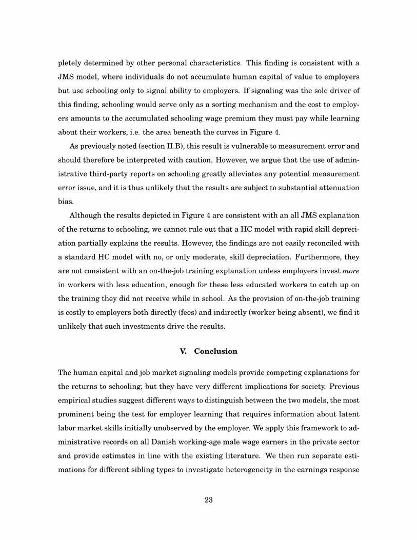
pletely determined by other personal characteristics. This finding is consistent with a

JMS model, where individuals do not accumulate human capital of value to employers

but use schooling only to signal ability to employers. If signaling was the sole driver of

this finding, schooling would serve only as a sorting mechanism and the cost to employ-

ers amounts to the accumulated schooling wage premium they must pay while learning

about their workers, i.e. the area beneath the curves in Figure 4.

As previously noted (section II.B), this result is vulnerable to measurement error and

should therefore be interpreted with caution. However, we argue that the use of admin-

istrative third-party reports on schooling greatly alleviates any potential measurement

error issue, and it is thus unlikely that the results are subject to substantial attenuation

bias.

Although the results depicted in Figure 4 are consistent with an all JMS explanation

of the returns to schooling, we cannot rule out that a HC model with rapid skill depreci-

ation partially explains the results. However, the findings are not easily reconciled with

a standard HC model with no, or only moderate, skill depreciation. Furthermore, they

are not consistent with an on-the-job training explanation unless employers invest more

in workers with less education, enough for these less educated workers to catch up on

the training they did not receive while in school. As the provision of on-the-job training

is costly to employers both directly (fees) and indirectly (worker being absent), we find it

unlikely that such investments drive the results.

V. Conclusion

The human capital and job market signaling models provide competing explanations for

the returns to schooling; but they have very different implications for society. Previous

empirical studies suggest different ways to distinguish between the two models, the most

prominent being the test for employer learning that requires information about latent

labor market skills initially unobserved by the employer. We apply this framework to ad-

ministrative records on all Danish working-age male wage earners in the private sector

and provide estimates in line with the existing literature. We then run separate esti-

mations for different sibling types to investigate heterogeneity in the earnings response

23

from ability proxies of different quality; thereby creating the link from the dominant

empirical strategy within the existing literature to twins-based estimation of employer

learning.

The large sample of Danish male twins, combined with detailed information on school-

ing and earnings, enables us to perform a more direct and precise test for employer learn-

ing compared to existing empirical evidence based on twin data. We study how earnings

differences vary with work experience over the early part of the working career for MZ

and DZ twins. The results show a decline in the returns to years of schooling differences

for MZ twins relative to DZ twins of 0.3 percent per year in the labor market. This find-

ing is consistent with some degree of job market signaling while not easily reconciled

with an explanation of private financial returns to schooling based on human capital

accumulation alone. When we define schooling as high school and college completion,

respectively, the results are qualitatively similar, although imprecisely estimated on the

college margin.

We use the sample of MZ twins to assess the relative importance of JMS for the

private financial returns to schooling and the speed with which employers learn about

initially unobserved ability components. For years of schooling and high school comple-

tion the return to schooling differences among MZ twins decreases during the first 10 to

15 years of work experience and seems to stabilize at a level close to zero. The rate of

convergence of MZ twin earnings provides a lower bound for the speed with which earn-

ings adjust if twins with less schooling do not receive (or benefit) more from on-the-job

training than their better educated co-twin. In that case, the rate of convergence could

be either positively or negatively biased.

Taken at face value, the results obtained from the sample of MZ twins show that

almost the entire private financial returns to an extra year of schooling or high school

completion are earned during the first 10 to 15 years in the labor market. This suggests

that JMS explains a substantial part of the returns to schooling and that employers

quickly learn about true abilities. However, a human capital model with rapid skill

depreciation could be part of the explanation as well. But the results are inconsistent

with a standard HC model that assumes no, or only little, skill depreciation. In contrast

to the results for years of schooling and high school completion, the estimated return to

24

college completion is persistent and fairly constant but it is imprecisely estimated.

References

Albrecht, J. W. (1981, February). A procedure for testing the signalling hypothesis. Jour-

nal of Public Economics 15(1), 123–132.

Altonji, J. G. and C. R. Pierret (1997, November). Employer learning and statistical

discrimination. NBER Working Papers 6279, National Bureau of Economic Research,

Inc.

Altonji, J. G. and C. R. Pierret (2001, February). Employer learning and statistical dis-

crimination. The Quarterly Journal of Economics 116(1), 313–350.

Arcidiacono, P., P. Bayer, and A. Hizmo (2010, October). Beyond signaling and human

capital: Education and the revelation of ability. American Economic Journal: Applied

Economics 2(4), 76–104.

Ashenfelter, O. and A. Krueger (1994). Estimates of the economic return to schooling

from a new sample of twins. The American Economic Review 84(5), pp. 1157–1173.

Bauer, T. K. and J. P. Haisken-DeNew (2001). Employer learning and the returns to

schooling. Labour Economics 8(2), 161 – 180. <ce:title>First World Conference of

Labour Economists, EALE-SOLE</ce:title>.

Bedard, K. (2001). Human capital versus signaling models: University access and high

school dropouts. Journal of Political Economy 109(4), 749.

Behrman, J. R. and M. R. Rosenzweig (1999). “ability” biases in schooling returns and

twins: a test and new estimates. Economics of Education Review 18(2), 159 – 167.

Bound, J. and G. Solon (1999). Double trouble: on the value of twins-based estimation of

the return to schooling. Economics of Education Review 18(2), 169 – 182.

Card, D. (1999, April). The causal effect of education on earnings. In O. Ashenfelter

and D. Card (Eds.), Handbook of Labor Economics, Volume 3 of Handbook of Labor

Economics, Chapter 30, pp. 1801–1863. Elsevier.

25

Chevalier, A., C. Harmon, I. Walker, and Y. Zhu (2004). Does education raise productivity,

or just reflect it? The Economic Journal 114(499), pp. F499–F517.

Dahl, C. M., D. l. Maire, and J. R. Munch (2013). Wage dispersion and decentralization

of wage bargaining. Journal of Labor Economics 31(3), pp. 501–533.

Farber, H. S. and R. Gibbons (1996). Learning and wage dynamics. The Quarterly Jour-

nal of Economics 111(4), pp. 1007–1047.

Foster, A. D. and M. R. Rosenzweig (1993). Information, learning, and wage rates in

low-income rural areas. Journal of Human Resources 28(4), 759–790.

Galindo-Rueda, F. (2003, May). Employer learning and schooling-related statistical dis-

crimination in britain. IZA Discussion Papers 778, Institute for the Study of Labor

(IZA).

Griliches, Z. (1979, October). Sibling Models and Data in Economics: Beginnings of a

Survey. Journal of Political Economy 87(5), S37–64.

Isacsson, G. (2004). Estimating the economic return to educational levels using data on

twins. Journal of Applied Econometrics 19(1), 99–119.

Jensen, V. M. and A. W. Rasmussen (2011). Danish education registers. Scandinavian

Journal of Public Health 39(7 suppl), 91–94.

Lang, K. and D. Kropp (1986). Human capital versus sorting: The effects of compulsory

attendance laws. The Quarterly Journal of Economics 101(3), pp. 609–624.

Lange, F. (2007). The speed of employer learning. Journal of Labor Economics 25, 1–35.

Lange, F. and R. Topel (2006). The Social Value of Education and Human Capital, Vol-

ume 1 of Handbook of the Economics of Education, Chapter 8, pp. 459–509. Elsevier.

Light, A. and A. McGee (2012, June). Employer learning and the

&quot;importance&quot; of skills. IZA Discussion Papers 6623, Institute for the

Study of Labor (IZA).

26

Mansour, H. (2012). Does employer learning vary by occupation? Journal of Labor

Economics 30(2), pp. 415–444.

Miller, P., C. Mulvey, and N. Martin (2006, October). The return to schooling: Estimates

from a sample of young australian twins. Labour Economics 13(5), 571–587.

Miller, P. W., C. Mulvey, and N. Martin (1995, June). What do twins studies reveal

about the economic returns to education? a comparison of australian and u.s. findings.

American Economic Review 85(3), 586–99.

Miller, P. W., C. Mulvey, and N. Martin (2004, October). A test of the sorting model of

education in australia. Economics of Education Review 23(5), 473–482.

Neumark, D. (1999). Biases in twin estimates of the return to schooling. Economics of

Education Review 18(2), 143 – 148.

Riley, J. G. (1979). Testing the educational screening hypothesis. Journal of Political

Economy 87(5), S227–52.

Sandewall, O., D. Cesarini, and M. Johannesson (2014). The co-twin methodology and

returns to schooling—testing a critical assumption. Labour Economics 26(0), 1 – 10.

Wolpin, K. I. (1977). Education and screening. The American Economic Review 67(5),

pp. 949–958.

27

Tables

Table 1: Summary statistics

Non-twin Twin Diff.a

Background characteristics

Year of birth 1967.8 1968.2 -0.4**(4.7) (4.9) (0.080)

Schooling (years) 12.9 12.9 0.0(2.2) (2.3) (0.037)

First year in the labor market 1990.6 1990.8 -0.3**(6.7) (6.7) (0.109)

Age at entry into labor market 22.8 22.6 0.1(4.1) (4.1) (0.067)

Ability proxies

Brother’s earnings (age 30-39)b 51.8 51.8 -0.1(23.7) (24.3) (0.394)

Father’s schooling (years) 11.0 11.0 0.0(3.4) (3.4) (0.055)

Father’s earnings (age 30-49)b 57.9 57.3 0.6(25.2) (24.6) (0.534)

Individuals 158813 3889Standard deviations in parenthesesaStandard errors in parentheses

* < .05 ** < .01bPercentile position in the earnings distribution. Mean over the age range.

Note: The sample of twin brothers is restricted to birth cohorts 1960 − 1980 to make it comparable to thesample of non-twin brothers.

Table 2: Twin differences in years of completed schooling

Years diff. MZ twins DZ twins

0 3293 (43%) 2770 (25%)

(0,1] 2137 (28%) 3773 (34%)

(1,2] 919 (12%) 1464 (13%)

(2,3] 507 ( 7%) 825 ( 7%)

(3,4] 488 ( 6%) 1188 (11%)

(4,5] 309 ( 4%) 776 ( 7%)

(5,6] 54 ( 1%) 179 ( 2%)

(6,7] 3 ( 0%) 65 ( 1%)

(7,8] 0 ( 0%) 21 ( 0%)Column shares (percent) in parentheses.

Table 3: Distribution of schooling attainment of twin brothers in the estimation sample.

MZ twin pairs

Compulsory High school College

Compulsory 524 ( 7%)

High school 888 (12%) 3922 (51%)

College 64 ( 1%) 1067 (14%) 1245 (16%)

DZ twin pairs

Compulsory High school College

Compulsory 799 ( 7%)

High school 1976 (18%) 4942 (45%)

College 218 ( 2%) 1940 (18%) 1186 (11%)

In parentheses: share (in percent) of cell to total number of observation within twin type.

Table 4: The effects of schooling, father’s education, father’s earnings, and brother’s earnings on wages. Dependentvariable: Employment-corrected wage earnings; Experience measure: Potential experience. Year 0-15 after graduation.

OLS estimates.

All brothers Non-twin brothers DZ twins MZ twins

(1a) (1b) (2a) (2b) (3a) (3b) (4a) (4b) (5a) (5b)

Education (years) 0.0952** 0.0997** 0.0981** 0.102** 0.0938** 0.0971** 0.0744** 0.0771** 0.0849** 0.0951**(0.000588) (0.000596) (0.000764) (0.000774) (0.000593) (0.000597) (0.00379) (0.00382) (0.00512) (0.00519)

Education*Experience/10 -0.0289**

-0.0335**

-0.0333**

-0.0372**

-0.0288**

-0.0320**

-0.0146**

-0.0171**

-0.0253**

-0.0346**

(0.000540) (0.000557) (0.000717) (0.000732) (0.000542) (0.000547) (0.00292) (0.00290) (0.00408) (0.00416)Father’s education (10 years) 0.0440** -

0.0694**(0.00184) (0.00306)

Father’s education*Experience/10 0.112**(0.00313)

Father’s earningsa 0.0313** -0.00637**

(0.000792) (0.00134)Father’s earnings*Experience/10 0.0377**

(0.00140)Brother’s earningsb 0.0301** -

0.00386**0.0466** 0.0114 0.101** 0.00788

(0.000679) (0.00103) (0.00557) (0.00783) (0.00647) (0.00990)Brother’s earnings*Experience/10 0.0336** 0.0318** 0.0850**

(0.00112) (0.00751) (0.00958)Spouse 0.0585** 0.0579** 0.0583** 0.0576** 0.0578** 0.0574** 0.0465** 0.0465** 0.0361** 0.0349**

(0.00104) (0.00104) (0.00132) (0.00131) (0.00104) (0.00104) (0.00724) (0.00723) (0.00827) (0.00828)# Kids -

0.00543**-

0.00504**-

0.00485**-

0.00457**-

0.00571**-

0.00581**(0.000636) (0.000635) (0.000808) (0.000807) (0.000637) (0.000636)

Year ! ! ! ! ! ! ! ! ! !

Industry, first job ! ! ! ! ! ! ! ! ! !

Experience (3rd order polynomial) ! ! ! ! ! ! ! ! ! !

N 1410269 1410269 846441 846441 1376539 1376539 38766 38766 24617 24617R2 0.373 0.375 0.370 0.372 0.378 0.380 0.537 0.538 0.562 0.568Standard errors in parenthesesStandard errors clustered by sibling group* p<0.05, ** p<0.01aThe average relative position in the wage distribution between ages 30 and 49. The relative position of individual earnings each year is calculatd as the value corresponding to the

percentile in the earnings distribution of the entire population of Danish working-age males, who are employed in the private sector and employed for at least 50% of the year. Thus,everyone is given a value between 1 and 100. This relative-earnings variable is then standardized to ease interpretation.bThe average relative position in the wage distribution between ages 30 and 39 calculated in the same way as father’s earnings.

Table 5: Cross-sectional and between-twins difference estimates of log earningsa

Twin fixed effects

Individuals DZ twins MZ twins

18-35 36-45 18-35 36-45 18-35 36-45

Schooling (years) 0.0315*** 0.0414*** 0.0229*** 0.0244*** 0.00995*** 0.00697(0.00163) (0.00235) (0.00289) (0.00397) (0.00350) (0.00528)

Age 0.0716*** 0.0384(0.00707) (0.0249)

Age2 -0.000969*** -0.000469(0.000122) (0.000312)

Spouse 0.0586*** 0.103*** 0.0511*** 0.0978*** 0.0164 0.0352*(0.00614) (0.0103) (0.00980) (0.0165) (0.0109) (0.0182)

Constant -1.645*** -1.243** -0.00317 0.0163 0.0000289 0.0156(0.100) (0.498) (0.00688) (0.0114) (0.00670) (0.0133)

Observations 40786 21856 12306 7017 8087 3911R2 0.132 0.103 0.029 0.046 0.004 0.005Standard errors in parenthesesStandard errors clustered at twin-pair level* p<0.1, ** p<0.05, *** p<0.01aNet of year fixed effects obtained from the entire population of working-age, private-sector, male wage earners, who

were employed in a full time job for at least six months during the year of observation.

Table 6: Twin FE estimation of returns to schooling. OLS regressions ofbetween-twins earnings differences from a sample of MZ and DZ twin brothers.

Dependent variable: ∆ Log wagea

Schooling variable: Years Levels (0, 1, 2) High school (0/1) College (0/1)

∆ Schooling (years) 0.0841*** 0.254*** 0.360*** 0.190***(0.00484) (0.0175) (0.0277) (0.0235)

Potential work experience (years) -0.00119 -0.00146 -0.00161 -0.00236*(0.00142) (0.00143) (0.00145) (0.00142)

∆ Schooling · experience -0.00487*** -0.00845*** -0.0289*** 0.0145***(0.000682) (0.00254) (0.00357) (0.00355)

MZ twin pair (0/1) 0.0120 0.00984 0.0123 0.00496(0.0136) (0.0140) (0.0145) (0.0146)

∆ Schooling · MZ 0.00993 0.00549 0.0234 -0.00467(0.00861) (0.0308) (0.0498) (0.0397)

Experience · MZ -0.00164 -0.00135 -0.00137 -0.000489(0.00205) (0.00208) (0.00209) (0.00208)

∆ Schooling · experience · MZ -0.00264** -0.00802* -0.00754 -0.0149**(0.00118) (0.00442) (0.00632) (0.00629)

∆ Spouse 0.0318*** 0.0240*** 0.0519*** 0.0357***(0.00849) (0.00842) (0.00910) (0.00818)

Constant 0.0146 0.0150 0.0176* 0.0174*(0.00964) (0.00988) (0.0103) (0.0103)

Observations 18771 18771 18771 18771Standard errors in parenthesesStandard errors clustered at twin-pair level* p<0.1, ** p<0.05, *** p<0.01aNet of year fixed effects obtained from the entire population of working-age, private-sector, male wage earners, who were

employed in a full time job for at least six months during the year of observation.

Figures

Figure 1: Stylized illustration of main empirical specification (without controls)

t

∆w

0

slope: β2 + β3

slope: β3

β0 + β1

β0 + β4

slope: β2 + β3 + β6 + β7

slope: β3 + β6

β0 + β1 + β4 + β5

β0

DZ twinsMZ twins

Specification

∆jwft = β̃0 + β1∆jSf + β2∆jSf · tf + β3tf + β4MZf + β5∆jSf ·MZf + β6tf ·MZf

+ β7∆jSf · tf ·MZf + δ∆jX ft + εft

Average returns to schooling:∂∆w

∂∆S= β1 + β2t+ β5MZ + β7t ·MZ

Slope in the returns to schooling:∂2∆w

∂∆S ∂t= β2 + β7MZ

Diff. in slopes between MZ and DZ:∂3∆w

∂∆S ∂t ∂MZ= β7

Figure 2: Twin mean wage differences over years after graduation from highestcompleted level of schooling. By schooling differences and twin type.

500

600

700

800

900

-.1

0

.1

.2

.3

0 5 10 15 0 5 10 15

MZ twins DZ twins

Diff. schooling Same schoolingsamp. size (right)

# tw

in p

airs

D w

age*

(lo

g-po

ints

)

Years after graduation

Total number of twin-pair observations in graph: 8K (MZ) 11K (DZ)*Log wage net of year fixed effects (from full-pop distribution)

Figure 3: Interquartile wage range for all Danish male, private-sector, full-timeemployeesa

80

100

120

140

160

Inte

rqua

rtile

wag

e ra

nge

(DK

K/1

000)

0 5 10 15 20 25

Years since graduation

1985 19901993 19982001 2005

Note: The 1985 graph only extends until 13 years after graduation because the administrativeeducational register with third-party reports on graduation date starts in 1971.aObtained from the entire population of working-age, private-sector, male wage earners, whowere employed in a full time job for at least six months during the year of observation.

Figure 4: OLS estimation of between-twin earnings differences on between-twinschoooling differences (twin FE) on the sample of MZ twin pairs. Estimates obtained

using four different definitions of schooling attainment.

0

.05

.1

.15

One

ext

ra y

ear

0 2 4 6 8 10 12 14Work experience

0

.1

.2

.3

.4

One

ext

ra le

vel

0 2 4 6 8 10 12 14Work experience

0

.2

.4

.6

Hig

h sc

hool

0 2 4 6 8 10 12 14Work experience

0

.1

.2

.3

Col

lege

0 2 4 6 8 10 12 14Work experience

Note: 95 percent confidence bands in gray. Standard errors clustered by twin pair.

Appendix

A. Orthogonality results

Table 7: The effects of schooling, father’s education, father’s earnings, and brother’s earnings on wages. Uses only thepart of the variation in father and brother variables that is independent of schooling and all other regressors.

Dependent variable: Employment-corrected wage earnings; Experience measure: Potential experience. Years 0-15after graduation. OLS estimates.

All brothers Non-twin brothers DZ twins MZ twins

(1a) (1b) (2a) (2b) (3a) (3b) (4a) (4b) (5a) (5b)

Education (years) 0.0963** 0.0962** 0.101** 0.101** 0.0965** 0.0964** 0.0754** 0.0751** 0.0863** 0.0882**(0.000585) (0.000584) (0.000760) (0.000759) (0.000589) (0.000588) (0.00379) (0.00379) (0.00515) (0.00515)

Education*Experience/10 -0.0287**

-0.0286**

-0.0329**

-0.0328**

-0.0288**

-0.0287**

-0.0147**

-0.0144**

-0.0249**

-0.0267**

(0.000540) (0.000539) (0.000717) (0.000715) (0.000542) (0.000538) (0.00293) (0.00291) (0.00410) (0.00403)Father’s education (10 years) 0.0147** -

0.0128**(0.000580) (0.000981)

Father’s education*Experience/10 0.0272**(0.00101)

Father’s earningsa 0.0306** 0.00296*(0.000768) (0.00131)

Father’s earnings*Experience/10 0.0277**(0.00138)

Brother’s earningsb 0.0287** 0.00276** 0.0398** 0.0202** 0.0862** 0.00814(0.000670) (0.00102) (0.00487) (0.00714) (0.00570) (0.00991)

Brother’s earnings*Experience/10 0.0257** 0.0179* 0.0721**(0.00111) (0.00710) (0.0102)

Spouse 0.0585** 0.0582** 0.0583** 0.0580** 0.0584** 0.0582** 0.0482** 0.0481** 0.0404** 0.0397**(0.00104) (0.00104) (0.00132) (0.00131) (0.00105) (0.00104) (0.00725) (0.00724) (0.00832) (0.00831)

# Kids -0.00572**

-0.00563**

-0.00531**

-0.00527**

-0.00568**

-0.00571**

(0.000635) (0.000635) (0.000808) (0.000808) (0.000638) (0.000637)Year ! ! ! ! ! ! ! ! ! !

Industry, first job ! ! ! ! ! ! ! ! ! !

Experience (3rd order polynomial) ! ! ! ! ! ! ! ! ! !

N 1410269 1410269 846441 846441 1376539 1376539 38766 38766 24617 24617R2 0.373 0.374 0.370 0.371 0.378 0.379 0.537 0.537 0.561 0.565Standard errors in parenthesesStandard errors clustered by sibling group* p<0.05, ** p<0.01aThe average relative position in the wage distribution between ages 30 and 49. The relative position of individual earnings each year is calculatd as the value corresponding to the

percentile in the earnings distribution of the entire population of Danish working-age males, who are employed in the private sector and employed for at least 50% of the year. Thus,everyone is given a value between 1 and 100. This relative-earnings variable is then standardized to ease interpretation.bThe average relative position in the wage distribution between ages 30 and 39 calculated in the same way as father’s earnings.