Signal Processing 85

ARTICLE IN PRESS

0165-1684/$ - se

doi:10.1016/j.sig

�Correspondi+972 4 8292795

E-mail addre

(T.G. Dvorkind

URL: http:/

Signal Processing 85 (2005) 177–204

www.elsevier.com/locate/sigpro

Time difference of arrival estimation of speech source in anoisy and reverberant environment

Tsvi G. Dvorkinda,�, Sharon Gannotb

aFaculty of Electrical Engineering, Technion, Technion City, 32000 Haifa, IsraelbSchool of Electrical Engineering, Bar-Ilan University, 52900 Ramat-Gan, Israel

Received 30 October 2003; received in revised form 23 September 2004

Abstract

Determining the spatial position of a speaker finds a growing interest in video conference scenarios where automated

camera steering and tracking are required. Speaker localization can be achieved with a dual-step approach. In the

preliminary stage a microphone array is used to extract the time difference of arrival (TDOA) of the speech signal. These

readings are then used by the second stage for the actual localization. In this work we present novel, frequency domain,

approaches for TDOA calculation in a reverberant and noisy environment. Our methods are based on the speech quasi-

stationarity property, noise stationarity and on the fact that the speech and the noise are uncorrelated. The

mathematical derivations in this work are followed by an extensive experimental study which involves static and

tracking scenarios.

r 2004 Elsevier B.V. All rights reserved.

Keywords: Source localization; Non-stationarity; Decorrelation; TDOA

1. Introduction

Determining the spatial position of a speakerfinds a growing interest in video conferencescenarios where automated camera steering andtracking are required. Microphone arrays, which

e front matter r 2004 Elsevier B.V. All rights reserve

pro.2004.09.014

ng author. Tel.: +972 4 8294751; fax:

.

sses: [email protected]

), [email protected] (S. Gannot).

/www.eng.biu.ac.il/~gannot.

are usually used for speech enhancement in a noisyenvironment [22], can be used for the task ofspeaker localization as well [3,6,8,9,11,20,27]. Therelated algorithms can be divided into two groups:single and dual-step approaches. In single stepapproaches the source location is determineddirectly from the measured data (i.e. the receivedsignals at the microphone array). In the dual-stepapproaches, the location estimate is obtained byapplying two algorithmic stages. First, time

difference (or time delay) of arrival (TDOA)estimates are obtained from different microphone

d.

www.elsevier.com/locate/sigpro

ARTICLE IN PRESS

T.G. Dvorkind, S. Gannot / Signal Processing 85 (2005) 177–204178

pairs. Then, these TDOA readings are used fordetermining the spatial position of the source.

Single step approaches can be further dividedinto two groups. The first group is the high-resolution spectral estimation methods. The well-known multiple signal classification (MUSIC)algorithm [35] is a member of this group. So isthe work in [21] which considers direction ofarrival (DOA) estimation with a uniform circulararrays that outperforms MUSIC-like algorithmsat low signal-to-noise ratio (SNR) for similarcomputational loads. Though the mentionedalgorithms can perform DOA estimation of multi-ple sources they are mainly suited for narrow-bandsignals. We note, however, that extension of thosealgorithms for a wide-band signals do exist. See forexample [12,40]. In the second group of single stepapproaches we find the maximum-likelihood (ML)algorithms, which estimate the source locus byapplying the ML criterion. Usually, the MLformulation leads to algorithms involving max-imization of the output power of a beamformersteered to potential source locations (i.e.[3,6,8,9,11]).

In the dual-step approaches group, the firstalgorithmic stage involves TDOA estimation fromspatially separated microphone pairs. The max-

imum-likelihood generalized cross correlation (ML-GCC)1 method presented by Knapp and Carter[27] is considered to be the classical solution forthis algorithmic stage. However, the GCC methodassumes a reverberant-free model such that theacoustical transfer function (ATF), which relatesthe source and each of the microphones, is a puredelay. Champagne et al. showed this approxima-tion to be inaccurate in reverberant conditions,which frequently occur in enclosed environments[7]. Consequently, algorithms for improving theGCC method in presence of room reverberationwere suggested [5,38]. Unfortunately, the GCCmethod suffers from another model inaccuracy. Itis assumed by the GCC model that the noise fieldis uncorrelated, an assumption which usually doesnot hold. Thus, the GCC method cannot distin-guish between the speaker and a directionalinterference, as it tends to estimate the TDOA of

1For brevity we will simply notate this by GCC.

the stronger signal. Directional interference usual-ly occurs when a point source, e.g. computer fan,projector or a ceiling fan, exists. The authors in[31] suggested discriminating speaker from direc-tional noise with a Gaussian mixture model. Adifferent approach was presented in [10,30], wherehigher order statistics (HOS) was employed forTDOA estimation of a non-Gaussian source andcorrelated Gaussian noise.Recently, subspace methods were suggested for

TDOA estimation. Assuming spatially uncorre-lated noise, Benesty suggested a time domainalgorithm for estimating the (truncated to shorterlength) impulse responses for TDOA extraction[2]. Extension of that work, for spatially correlatednoise was presented by Doclo and Moonen [13,15].Assuming that the noise correlation matrix isknown (using a voice activity detector (VAD)), theauthors presented a time domain algorithm forTDOA estimation using a generalized eigenvalue

decomposition (GEVD) approach and a pre-whitening approach.In this work, we tackle the TDOA estimation

problem. Hence, the proposed solutions aremembers of the dual-step approaches. We addressthe TDOA extraction based on a single micro-phone pair. The second algorithmic stage, i.e. theactual localization based on multiple TDOAreadings which are extracted from additionalmicrophone pairs [4,18,25], is not addressed inthis work. Our model assumptions considerreverberation and spatially correlated noise sce-narios [17,19]. Specifically, we consider a singlespeaker in a stationary noise environment. In [22]the speaker’s ATF-s ratio was used as part of abeamformer in a speech enhancement application.Here, we exploit this quantity for the sourcelocalization application. Particularly, we show thatthe TDOA reading can be extracted from thelocation of the maximal peak in the correspondingimpulse response. Similar to [22] and the precedingwork by Shalvi and Weinstein [37] we also assumethat the interfering noise is relatively stationary,and present a framework where the ATF-s ratioand a noise related term are estimated simulta-neously without any VAD employment. Quasi-stationarity of the speech and stationarity of thenoise are exploited to derive batch and recursive

ARTICLE IN PRESS

T.G. Dvorkind, S. Gannot / Signal Processing 85 (2005) 177–204 179

solutions. The importance of the recursive solutionmanifests itself in tracking scenarios, where theestimated ATF-s ratio and noise statistics mightslowly vary with time. Following the work in [41],we have additionally exploited the fact that there isno correlation between the speaker and thedirectional noise. The authors in [41] showed thatin an application of signal separation, imposing adecorrelation criterion on the estimated signalsresults in ATF-s ratio estimation. The authorsfurther suggested exploiting speech non-stationar-ity, resulting in a set of decorrelation equations.However, the obtained equation set is nonlinear,and due to this nonlinearity an inherent frequency

permutation ambiguity results [32]. The authors in[41] did not give a closed form solution for theresulting, frequency domain, nonlinear equationset. Instead, it was suggested to solve the problemiteratively, by assuming a simplified finite impulseresponse (FIR) model for the mixing channels andsolving in the time domain. To maintain simplicityof the solution, we are solving the problem in thefrequency domain. Furthermore, we do notassume the simplified mixing channel.

The obtained decorrelation equations are closelyrelated to blind source separation (BSS) problems.Gannot and Yeredor considered the case ofinstantaneous mixture of a non-stationary signalwith a stationary noise [23], where joint diagona-lization of correlation matrices is carried out in thetime domain. Considering a convolutive mixture(due to room reverberation), researchers suggestedsolving the nonlinear frequency domain decorrela-tion equations by applying joint diagonalization ofthe PSD matrices obtained from different timeepoches. Special attention is given to the inherentfrequency permutation problem, which is usuallysolved by imposing an FIR constraint on theseparating ATF-s [32,36] or (equivalently) impos-ing smoothness in the frequency domain [34]. Inour contribution we exploit the stationarity of oneof the sources (the directional noise) to resolvefrequency permutations. No FIR constraint isemployed, and the estimated ATF-s ratio isexploited for TDOA extraction. Our simulationstudy shows that the decorrelation constraintpresents improved TDOA estimation for the batchmethods at low SNR conditions.

Special emphasis is given for deriving a recursivesolution applicable for tracking scenarios. Sincethe involved decorrelation equation set is non-linear, we present a general framework for anapproximate recursive solution of a nonlinearequation set. The method notated by recursive

Gauss (RG) is applied to the nonlinear decorrela-tion equations, resulting in a solution applicablefor tracking scenarios. Opposed to the GCC-basedmethods, our solutions deal with reverberantenvironment and correlated noise field. Opposedto the subspace methods [2,15], the proposedalgorithms are conducted in the frequency domain,resulting in computationally more efficient imple-mentations which do not rely on a VAD for priorknowledge of the noise characteristics. Further-more, simulation study shows that the suggestedalgorithms are suitable for tracking scenarios,while the subspace method fails to lock on theTDOA readings, which constantly change due tosource movement.The outline of this work is as follows. In Section

2 we present the model assumptions and suggestthe use of ATF-s ratio quantity for TDOAestimation. Section 3 presents the TDOA estima-tion algorithms, exploiting speech quasi-stationar-ity, noise stationarity and the fact that there is nocorrelation between the speech and the noise.Extensive experimental study is presented inSection 4. Finally, several practical considerationsare presented in Section 5.

2. Problem formulation and motivation

In this section the problem is formulated and thebasic assumptions are presented. By analyticalexpression and by simulation study, we justify theuse of ATF-s ratio for TDOA extraction.

2.1. Basic model assumptions

Define a set of M microphones for which themeasured signal at the mth microphone, zmðtÞ; is

zmðtÞ ¼ amðtÞ � sðtÞ þ nmðtÞ; m ¼ 1; . . . ;M ; (1)

where * stands for convolution, sðtÞ is the sourcesignal and nmðtÞ is the interference signal at the mth

ARTICLE IN PRESS

2We note that hmðtÞ is a non-causal impulse response, since

ATF-s are usually non-minimum phase. Thus, evaluation of the

ATF-s ratio in the Z domain, contains poles both inside and

outside the unit circle.3The reverberation time is the time for the acoustic energy to

drop by 60 dB from its original value. This time is set using

Eyring formula [28]: T r ¼ ð�13:82=cðL�1x þ L�1

y þ L�1z Þ ln bÞ

with b the reflection coefficient ðb 2 ð0; 1ÞÞ;Lx;Ly;Lz are the

rectangular room dimensions and c is the sound propagation

speed (approximately 340m/s in air).


microphone. t stands for the discrete time index.Naturally, we assume that the interference signal isuncorrelated with the source signal. amðtÞ is animpulse response from the desired speech source tothe mth microphone. When nmðtÞ is a directionalinterference, we can state

nmðtÞ ¼ bmðtÞ � nðtÞ; m ¼ 1; . . . ;M ; (2)

where bmðtÞ is the impulse response between thenoise nðtÞ and the mth microphone. sðtÞ is assumedto be quasi-stationary, while the interferencesignals are assumed to be stationary (or at leastmore stationary than the speech signal sðtÞ). Thiswill be defined more precisely in the sequel.

2.2. Usage of ATF-s ratio for TDOA extraction

Let AmðoÞ be the frequency response of the mthimpulse response amðtÞ: Define

HmðoÞ9AmðoÞA1ðoÞ

(3)

the ATF-s ratio and its corresponding impulseresponse hmðtÞ: Usually, the desired TDOA valuecan be extracted from hmðtÞ by estimating its peakvalue location. Assume that

AmðoÞ ¼ an0e�jon0 þ

XLm

i¼1

anie�joni ; m ¼ 2 . . .M ;

A1ðoÞ ¼ bp0e�jop0 þ

XL1

i¼1

bpie�jopi

with an0 ;bp0and n0; p0 being the amplitudes and

the delays of the largest peaks (not necessarilyrelating to the first arrival peaks) of amðtÞ and a1ðtÞ;respectively. Note that we have omitted themicrophone indices dependence of the gains andthe delays for brevity. Lm and L1 are the lengths ofthe above impulse responses. The respective ATF-sratio can be stated as

HmðoÞ ¼an0e

�jon0

bp0e�jop0

emðoÞ;

emðoÞ ¼1þ

PLm

i¼1 ðanie�joni=an0e

�jon0 Þ

1þPL1

i¼1 ðbpie�jopi=bp0

e�jop0Þ:

At low reverberation, where jan0 jbjanij and

jbp0jbjbpi

j; ðia0Þ the error multiplicative term

emðoÞ tends to be close to 1, and the peak of thecorresponding hmðtÞ can be used to determinethe TDOA.2 Experimental study supports thisapproach.

2.2.1. Preliminary simulation

To justify the use of the ATF-s ratio for TDOAextraction the following simulation was carriedout. In a rectangular room with dimensions[4,7,2.75], 125 possible source locations wereconsidered, by uniformly distributing 5 positionsalong each axis. A pair of microphones was placednear the center of the room at coordinates[2,3.5,1.375] and [1.7,3.5,1.375]. Using the imagemethod [1,33], the ATF-s relating each possiblesource position to each microphone were simu-lated. Six reverberation values, denoted by T r;

3

were considered. Ranging from low reverberationconditions ðT r ¼ 0:1 sÞ to moderate conditionsðT r ¼ 0:6 sÞ: Two approaches were examined.TDOA estimation using ATF-s ratio, and TDOAestimation using the GCC method [27]. Assume anoise-free case, such that zmðtÞ ¼ amðtÞ � sðtÞ; m ¼

1; . . . ;M : The ATF-s ratio can be estimated fromthe cross-PSD divided by the auto-PSD:

Fzmz1ðoÞFz1z1ðoÞ

¼AmðoÞA�

1ðoÞFssðoÞA1ðoÞA�

1ðoÞFssðoÞ¼ HmðoÞ; (4)

where FssðoÞ is the speech PSD at the estimationframe and * stands for conjugation. In practice,however, PSD-s will be estimated using a finitesupport observation window. Suppose that Welchmethod [42] is applied for the PSD estimation,using window wðtÞ of length P. Denote by Fzizj

ðoÞthe cross-PSD estimate of zi with zj : Note thatlimP!1ðFzmz1 ðoÞ=Fz1z1ðoÞÞ ¼ HmðoÞ: However,for a finite length analysis window wðtÞ (i.e. P isfinite) ðFzmz1 ðoÞ=Fz1z1ðoÞÞaHmðoÞ as the PSD

ARTICLE IN PRESS

0.1 0.15 0.2 0.25 0.3 0.35 0.4 0.45 0.5 0.55 0.60.1

0.15

0.2

0.25

0.3

0.35

0.4

0.45P=4096, overlap=2048

RM

SE

[sam

ple]

Tr[sec]

RatioGCC

0.1 0.15 0.2 0.25 0.3 0.35 0.4 0.45 0.5 0.55 0.60

10

20

30

40

50

60

70

80

90P=4096, overlap=2048

Ano

mal

y%

Tr[sec]

RatioGCC

Fig. 1. Simulative model test. Long observation frame.

5This is a reasonable value considering the microphone

separation distance and the stated sampling rate. This value was


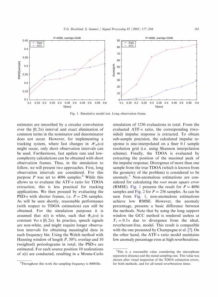
estimates are smoothed by a circular convolutionover the ½0; 2pÞ interval and exact elimination ofcommon terms in the nominator and denominatordoes not occur. However, for implementing atracking system, where fast changes in HmðoÞmight occur, only short observation intervals canbe used. Furthermore, fast update rate and low-complexity calculations can be obtained with shortobservation frames. Thus, in the simulation tofollow, we will present two approaches. First, longobservation intervals are considered. For thispurpose P was set to 4096 samples.4 While thisallows us to evaluate the ATF-s ratio for TDOAextraction, this is less practical for trackingapplications. We then proceed by evaluating thePSD-s with shorter frames, i.e. P ¼ 256 samples.As will be seen shortly, reasonable performance(with respect to TDOA estimation) can still beobtained. For the simulation purposes it isassumed that sðtÞ is white, such that FssðoÞ isconstant 8o 2 ½0; 2pÞ: In practice, speech signalsare non-white, and might require longer observa-tion intervals for obtaining meaningful data ineach frequency bin. Using the Welch method withHanning window of length P, 50% overlap and 10(weighted) periodograms in total, the PSD-s areestimated. For each source position 10 realizationsof sðtÞ are conducted, resulting in a Monte-Carlo

4Throughout this work the sampling frequency is 8000Hz.

simulation of 1250 evaluations in total. From theevaluated ATF-s ratio, the corresponding (two-sided) impulse response is extracted. To obtainsub-sample precision, the calculated impulse re-sponse is sinc-interpolated on a finer 0.1 sampleresolution grid (i.e. using Shannon interpolationscheme). Finally, the TDOA is evaluated byextracting the position of the maximal peak ofthe impulse response. Divergence of more than onesample from the true TDOA (which is known fromthe geometry of the problem) is considered to beanomaly.5 Non-anomalous estimations are con-sidered for calculating the root mean square error

(RMSE). Fig. 1 presents the result for P ¼ 4096samples and Fig. 2 for P ¼ 256 samples. As can beseen from Fig. 1, non-anomalous estimationsachieve low RMSE. However, the anomalypercentage, presents a basic difference betweenthe methods. Note that by using the long supportwindow the GCC method is rendered useless atT r ¼ 0:3 s due to divergence from the ideal,reverberant-free, model. This result is compatiblewith the one presented by Champagne et al. [7]. Onthe other hand, the ATF-s ratio model maintainslow anomaly percentage even at high reverberations.

chosen after visual inspection of the TDOA estimation errors,

for both methods, and for all tested reverberation times.

ARTICLE IN PRESS

0.1 0.15 0.2 0.25 0.3 0.35 0.4 0.45 0.5 0.55 0.60.1

0.15

0.2

0.25

0.3

0.35P=256, overlap=128

RM

SE

[sam

ple]

Tr[sec]

RatioGCC

0.1 0.15 0.2 0.25 0.3 0.35 0.4 0.45 0.5 0.55 0.60

5

10

15

20

25

30

35

40P=256, overlap=128

Ano

mal

y%

Tr[sec]

RatioGCC

Fig. 2. Simulative model test. Short observation frame.


Fig. 2 presents the TDOA estimation results basedon short observation interval. As can be seen, themethods still have small RMSE. From thepresented anomaly percentage we can see that byevaluating the PSD-s with small P we can actuallyimprove the GCC robustness to reverberation(note that the analysis carried out in [7] exploitedlong observation frames). Examining the anomalypercentage for the ATF-s ratio method, we noticean increase for large T r values (up-till 37% at T r ¼

0:6 s; instead of 29% at the long frame case).However, we aim to mid range reverberation ofT r ¼ 0:220:3 s: Furthermore, the use of addi-tional, spatially separated microphone pairs,which will produce additional TDOA readings, isexpected to improve the actual localization. It isworth mentioning that the GCC method stillsuffers from another modeling assumption: itassumes uncorrelated measurement noise. In thesequel, we will demonstrate that the GCC methodis rendered useless in the presence of correlatednoise and low SNR conditions, while thealgorithms derived in Section 3 present robustbehavior.

6Though our expressions consider a single directional

interference, all the derivations can be extended for a multiple

(stationary) interferers in a straight forward manner.

3. Algorithm derivation—TDOA

In this section we address the problem of ATF-sratio estimation. Quasi-stationarity of the speech

signal, stationarity of the noise signal and the factthat speech and noise signals are uncorrelated areexploited for deriving several algorithms.

3.1. Speech quasi-stationarity

An unbiased method for estimating HmðoÞ;exploiting the speech signal quasi-stationarity, wasfirst presented in [22], based on a method derivedin [37]. Noting that the speaker and the noisesource are uncorrelated, we can state the followingequation:

FzizjðoÞ ¼ AiðoÞA�

j ðoÞFssðoÞ

þ BiðoÞB�j ðoÞFnnðoÞ ð5Þ

with Fzizjbeing the cross-PSD of zi and zj ; FssðoÞ

is the speech auto-PSD and FnnðoÞ is the noiseauto-PSD. BmðoÞ is the frequency response ofbmðtÞ:

6 Examining (5), we note that

Fzmz1ðoÞ �HmðoÞFz1z1ðoÞ ¼ Fb1mðoÞ; (6)

where

Fb1mðoÞ ¼ ðGmðoÞ �HmðoÞÞjB1ðoÞj2FnnðoÞ (7)

is a noise-only term, and we defineGmðoÞ9ðBmðoÞ=B1ðoÞÞ to be the noise ATF-s

ARTICLE IN PRESS


ratio. In practice, however, stationarity of thespeech signal can be assured only over shorttime intervals. Consider an observation intervalof length NP for which the noise signal canbe regarded stationary and the ATF-s timeinvariant, while the speech signal statistics ischanging. However, by dividing the observationinterval into N consecutive frames (of lengthP each), the speech signal is regarded stationaryfor each frame. Hence, notating the frame indexby n ¼ 1; . . . ;N the speech signal auto-PSDat the nth frame can be written as Fssðn;oÞ (thisis the quasi-stationarity assumption for speechsignals).

By evaluating (6) for each frame, an over-determined set of equations for HmðoÞ is ob-tained. This set can be solved by virtue of the least

squares (LS) method [26]. The resultant frequencydomain algorithm is now presented.

Exploiting the quasi-stationarity property of thespeech and defining

Fb1mðn;oÞ9Fzmz1ðn;oÞ

�HmðoÞFz1z1 ðn;oÞ; n ¼ 1; . . . ;N ;

where, Fzizjðn;oÞ is an estimate of the PSD of zi

and zj at the nth frame, Eq. (6) becomes a set ofequations for HmðoÞ: This overdetermined set forHmðoÞ can also be stated as

Fzmz1 ðn;oÞ ¼ HmðoÞFz1z1 ðn;oÞ þ Fb1mðoÞ

þ xðn;oÞ; n ¼ 1; . . . ;N ; ð8Þ

where, xðn;oÞ9Fb1mðn;oÞ � Fb1m

ðoÞ is an errorterm, which is minimized in the LS sense, usingthe overdetermined set (8). The noise-onlyterm Fb1m

ðoÞ which is regarded stationary, andthe ATF-ratio HmðoÞ; which is assumed to beslow time varying, are independent of the frameindex (n). We denote this set of equations (or theequivalent relation in (6)) as the first form of

stationarity (S1). The weighted LS (WLS) solution[26] to (8) is

HmðoÞ

Fb1mðoÞ

" #¼ ðAyWAÞ�1AyWFzmz1

ðoÞ (9)

with

A9

Fz1z1ð1;oÞ; 1

..

.

Fz1z1 ðN;oÞ; 1

2664

3775; Fzmz1

ðoÞ9

Fzmz1 ð1;oÞ

..

.

Fzmz1 ðN;oÞ

2664

3775:

W is an optional weight matrix and y stands forHermitian transpose. In practice, for a non-moving source, W is set to the identity matrix.Alternatively, using the same assumptions as

before and by evaluating the connection betweenFzmzm

ðoÞ and Fz1zmðoÞ a second form of stationarity

(S2) can be stated. Examine

Fzmzmðn;oÞ ¼ HmðoÞFz1zm

ðn;oÞ þ Fb2mðoÞ

þ x2ðn;oÞ; n ¼ 1; . . . ;N; ð10Þ

where Fb2mis also a stationary noise-only term

Fb2mðoÞ ¼ ðGmðoÞ �HmðoÞÞB1ðoÞB�

mðoÞFnnðoÞ

(11)

and similar to the definition of xðn;oÞ; we havethe error term x2ðn;oÞ9Fb2m

ðn;oÞ � Fb2mðoÞ; with

Fb2mðn;oÞ9Fzmzm

ðn;oÞ �HmðoÞFz1zmðn;oÞ:

This second form of stationarity has LS solutionsimilar to (9)

HmðoÞ

Fb2mðoÞ

" #¼ ðByWBÞ�1ByWFzmzm

ðoÞ (12)

with

B9

Fz1zmð1;oÞ; 1

..

.

Fz1zmðN ;oÞ; 1

2664

3775; Fzmzm

ðoÞ9

Fzmzmð1;oÞ

..

.

FzmzmðN;oÞ

2664

3775:

The importance of this second form of stationaritywill be clarified in the next subsection, where werelate it (and the first form of stationarity) to thedecorrelation criterion.

3.2. Decorrelation criterion

Until this point we estimated HmðoÞ based onnoise stationarity and the speech quasi-stationaritycharacteristics. Though the lack of correlationbetween the speech and the noise term was already

ARTICLE IN PRESS

7Indeed this is a difficulty, since permutations in each

frequency prevents consistent construction of HmðoÞ:


used in deriving (5) it is interesting to incorporatethis property directly as a part of the criterion.Namely, imposing the fact that the speaker and theinterference noise must be uncorrelated.

Our observations are a mixture of the filteredspeech smðtÞ9amðtÞ � sðtÞ and the noise nmðtÞ: Asfor directional noise nmðtÞ9bmðtÞ � nðtÞ; the cross-PSD matrix of the first and the mth microphonecan be written as

PðoÞ9Fz1z1ðoÞ Fz1zm

ðoÞ

Fzmz1ðoÞ FzmzmðoÞ

� �; (13)

where Fzizj¼ AiðoÞA�

j ðoÞFssðoÞ þ BiðoÞB�j ðoÞ

FnnðoÞ: Applying an unmixing transformationUðoÞ to ½Z1ðoÞ ZmðoÞ�T such that the outputPSD matrix RðoÞ ¼ UðoÞPðoÞUyðoÞ is diagonalyields decorrelated outputs. We show now that aby-product of the diagonalization process will leadus to an estimate of HmðoÞ: In particular, andwithout loss of generality, by setting

UðoÞ ¼u1ðoÞ �1

�u2ðoÞ 1

�

and constraining the off-diagonal elements of RðoÞto zero we obtain the (nonlinear) decorrelationcriterion

u�2ðoÞðFzmz1ðoÞ � u1ðoÞFz1z1 ðoÞÞ

¼ FzmzmðoÞ � u1ðoÞFz1zm

ðoÞ: ð14Þ

Note that (14) is a single (nonlinear) equation intwo unknowns. Eq. (14) was derived in [41], and itwas iteratively solved in the time domain for asimplified version of the mixing channel, wherethe problem was constrained to FIR decouplingfilters. The authors in [41] suggested to exploitspeech quasi-stationarity to obtain a set ofequations for u1ðoÞ and u2ðoÞ: Indeed, byexploiting the quasi-stationarity property of thespeech, Eq. (14) becomes a set of equations,obtained by evaluating the PSD-s at differentframe indices

u�2ðoÞðFzmz1

ðoÞ � u1ðoÞFz1z1ðoÞÞ

� FzmzmðoÞ � u1ðoÞFz1zm

ðoÞ ð15Þ

with

Fzmz1ðoÞ9

Fzmz1 ð1;oÞ

..

.

Fzmz1 ðN;oÞ

2664

3775;

Fz1z1ðoÞ9

Fz1z1ð1;oÞ

..

.

Fz1z1ðN;oÞ

2664

3775;

FzmzmðoÞ9

Fzmzmð1;oÞ

..

.

FzmzmðN ;oÞ

2664

3775;

where N is the number of evaluated frames. ForNX2 we have enough equations to solve theproblem, though the expressions are still nonlinearin u1ðoÞ and u2ðoÞ: Simple assignment shows thatthe pair fu2ðoÞ ¼ GmðoÞ; u1ðoÞ ¼ HmðoÞg as wellas the pair fu1ðoÞ ¼ GmðoÞ; u2ðoÞ ¼ HmðoÞg solvesthe equations at hand. This is referred to as thefrequency permutation ambiguity problem7 [32].The authors in [41] did not present a solution to(15). In particular, they avoided the permutationproblem inherent in (15), by solving the problem(iteratively) in the time domain. In this contribu-tion we solve (15) directly to obtain an estimate forHmðoÞ: Furthermore, we tackle the permutationproblem by exploiting noise stationarity.

3.3. Decorrelation algorithms

To maintain simplicity of the solution, we wishto solve the problem in the frequency domain. Themain attraction of the frequency domain approachis its ability to translate the problem fromconvolutive mixture to an instantaneous mixture.Noting that the equation set (15) is nonlinear inu2ðoÞ and u1ðoÞ; the Gauss method is employed(Appendix A). Though other search algorithmscan be applied, this method was chosen due to itssimplicity and since a simple way for deriving arecursive solution for it exists. This recursive

ARTICLE IN PRESS


solution, which we will address in the sequel,enables tracking of a moving source.

Fig. 3. Linear decorrelation (LD) algorithm. Batch solution.
3.3.1. Linear solution
We start by presenting a simple and non-iterative way for obtaining an estimate of u1ðoÞ ¼HmðoÞ from set (15). Special attention will begiven to avoid the permutation problem, i.e. thesolution u1ðoÞ ¼ GmðoÞ:

Experimental results revealed that the first (andsecond) form of stationarity perform well atreasonable SNR, but at negative SNR values theirestimate of HmðoÞ deteriorates. On the otherhand, it is assumed that for negative SNR values,the estimated noise bias terms (Fb1m

ðoÞ in (9) and

Fb2mðoÞ in (12)) can be reliably obtained.8 Using (7)

and (11) it is evident that

Fb2mðoÞ

Fb1mðoÞ

¼ G�mðoÞ: (16)

Thus, a possible initialization for u�2ðoÞ is

u�2ðoÞ ¼

Fb2mðoÞ

Fb1mðoÞ

: (17)

This assignment has a twofold advantage. First,using this initialization, the set (15) becomes alinear set in u1ðoÞ: Thus, LS solution can beobtained

HmðoÞ ¼ ðVy V Þ�1V y½Fzmzm

ðoÞ � u�2ðoÞFzmz1

ðoÞ�;

(18)

where

V 9Fz1zmðoÞ � u�

2ðoÞFz1z1ðoÞ

and u�2ðoÞ is set according to (17). Second, by

setting u�2ðoÞ ¼ G�

mðoÞ; u1ðoÞ must tend to becomeHmðoÞ; thus overcoming the frequency permuta-tion problem. The resultant algorithm is notatedby linear decorrelation (LD) and is summarized inFig. 3.

8In general, there is an inherent tradeoff in the algorithm.

While estimating noise bias terms and the speaker’s ATF-ratio

in a single LS formulation, an accurate solution for both cannot

be obtained for very high and very low SNR conditions

simultaneously.

The stated solution is a batch solution, i.e. allthe available data are used at once. A recursivesolution, directly applicable to the tracking pro-blem, will be presented in the sequel.

3.3.2. Decorrelation and first form of stationarity

We now present an iterative solution to (15)based on the Gauss method. In the previoussection the LD algorithm resolved the permutationproblem by simply relying on a proper initializa-tion for u2ðoÞ: An alternative approach (whichalso exploits noise stationarity), is to solve sets (15)and (8) simultaneously as one large LS problem.Concatenating these equations we get

Fz1zmðoÞ Fzmz1

ðoÞ �Fz1z1ðoÞ 0

Fz1z1ðoÞ 0 0 1

" #

Times

HmðoÞ

G�mðoÞ

HmðoÞG�mðoÞ

Fb1mðoÞ

2666664

3777775 �

FzmzmðoÞ

Fzmz1ðoÞ

" #; ð19Þ

where 0 and 1 stand for column vectors (of properdimensions) of zeros and ones, respectively.Denote the parameter set by

y9½HmðoÞ;G�mðoÞ;Fb1m

ðoÞ�T:

Denote the left-hand side of (19) by

hðyÞ9HmðoÞFz1zm

ðoÞ

Fz1z1ðoÞ

" #þ G�

mðoÞFzmz1

ðoÞ

0

" #

�HmðoÞG�mðoÞ

Fz1z1ðoÞ

0

" #

þ Fb1mðoÞ

0

1

" #: ð20Þ

ARTICLE IN PRESS


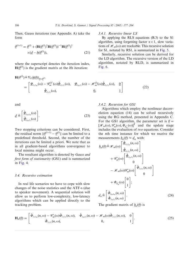
Then, Gauss iterations (see Appendix A) take theform

yðlþ1Þ¼ yðlÞ þ ðHðyðlÞÞyHðyðlÞÞÞ�1HðyðlÞÞy

�ðd � hðyðlÞÞÞ; ð21Þ

where the superscript denotes the iteration index,HðyðlÞÞ is the gradient matrix at the lth iteration:

HðyðlÞÞ9ry hðyÞjy¼yðlÞ

¼Fz1zm

ðoÞ � GðlÞ�

m ðoÞFz1z1ðoÞ; Fzmz1

ðoÞ �HðlÞm ðoÞFz1z1

ðoÞ; 0

Fz1z1ðoÞ; 0; 1

" #ð22Þ

and

d 9Fzmzm

ðoÞ

Fzmz1ðoÞ

" #: (23)

Two stopping criterions can be considered. First,the residual norm kyðlþ1Þ

� yðlÞk can be limited to apredefined threshold. Second, the number of theiterations can be limited a priori. We note that asin all gradient-based algorithms convergence tolocal minima might occur.

The resultant algorithm is denoted by Gauss and

first form of stationarity (GS1) and is summarizedin Fig. 4.

3.4. Recursive estimation

In real life scenarios we have to cope with slowchanges of the noise statistics and the ATF-s (dueto speaker movement). A sequential solution willallow us to perform low-complexity, low-latencyalgorithms which can be applied directly to thetracking problem.

HnðyÞ ¼Fz1zm

ðn;oÞ � G�mðoÞFz1z1 ðn;oÞ; Fzmz1 ðn;oÞ �

Fz1z1 ðn;oÞ;

"

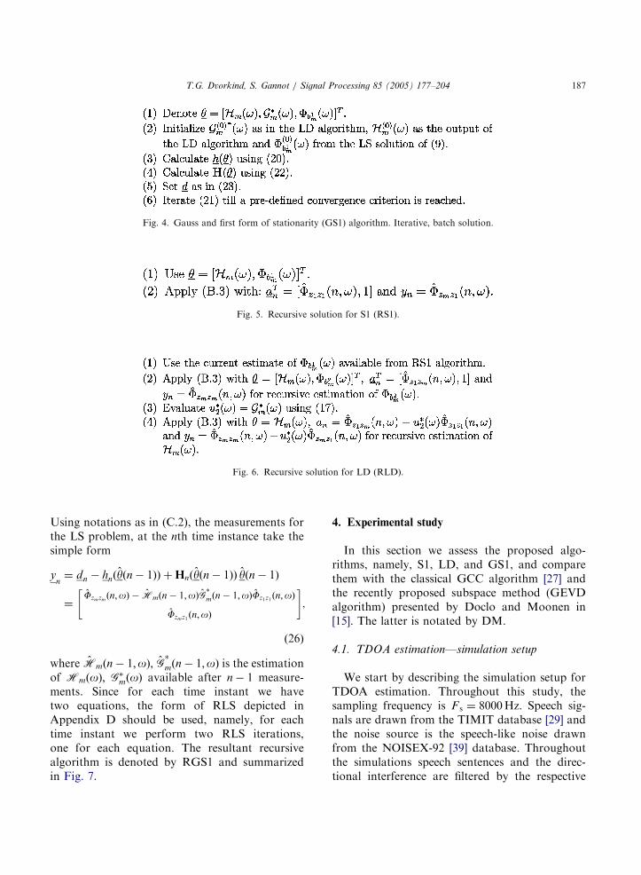
3.4.1. Recursive linear LS

By applying the RLS equations (B.3) to the S1algorithm, using forgetting factor ao1; slow varia-tions ofHmðoÞ are trackable. This recursive solutionfor S1, notated by RS1, is summarized in Fig. 5.Similarly, recursive solution can be derived for

the LD algorithm. The recursive version of the LDalgorithm, notated by RLD, is summarized inFig. 6.

3.4.2. Recursion for GS1

Algorithms which employ the nonlinear decorr-elation equation (14) can be solved recursivelyusing the RG method, presented in Appendix C.For the GS1 algorithm, the parameter set is y ¼

½HmðoÞ;G�mðoÞ;Fb1m

ðoÞ�T and the update stageincludes the evaluation of two equations. Considerthe nth time instance for which we receive themeasurements hnðyÞ � dn with:

hnðyÞ9HmðoÞFz1zm

ðn;oÞ

Fz1z1ðn;oÞ

" #

þ G�mðoÞ

Fzmz1ðn;oÞ

0

" #

�HmðoÞG�mðoÞ

Fz1z1 ðn;oÞ

0

" #

þ Fb1mðoÞ

0

1

" #;

dn9Fzmzm

ðn;oÞ

Fzmz1 ðn;oÞ

" #: (24)

The gradient matrix of hnðyÞ is

HmðoÞFz1z1 ðn;oÞ; 0

0; 1

#: (25)

ARTICLE IN PRESS

Fig. 4. Gauss and first form of stationarity (GS1) algorithm. Iterative, batch solution.

Fig. 5. Recursive solution for S1 (RS1).

Fig. 6. Recursive solution for LD (RLD).


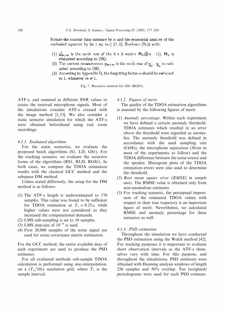
Using notations as in (C.2), the measurements forthe LS problem, at the nth time instance take thesimple form

yn¼ dn � hnðyðn � 1ÞÞ þHnðyðn � 1ÞÞ yðn � 1Þ

¼Fzmzm

ðn;oÞ � Hmðn � 1;oÞG�

mðn � 1;oÞFz1z1 ðn;oÞ

Fzmz1ðn;oÞ

" #;

ð26Þ

where Hmðn � 1;oÞ; G�

mðn � 1;oÞ is the estimationof HmðoÞ; G�

mðoÞ available after n � 1 measure-ments. Since for each time instant we havetwo equations, the form of RLS depicted inAppendix D should be used, namely, for eachtime instant we perform two RLS iterations,one for each equation. The resultant recursivealgorithm is denoted by RGS1 and summarizedin Fig. 7.

4. Experimental study

In this section we assess the proposed algo-rithms, namely, S1, LD, and GS1, and comparethem with the classical GCC algorithm [27] andthe recently proposed subspace method (GEVDalgorithm) presented by Doclo and Moonen in[15]. The latter is notated by DM.

4.1. TDOA estimation—simulation setup

We start by describing the simulation setup forTDOA estimation. Throughout this study, thesampling frequency is F s ¼ 8000Hz: Speech sig-nals are drawn from the TIMIT database [29] andthe noise source is the speech-like noise drawnfrom the NOISEX-92 [39] database. Throughoutthe simulations speech sentences and the direc-tional interference are filtered by the respective

ARTICLE IN PRESS

Fig. 7. Recursive solution for GS1 (RGS1).


ATF-s, and summed at different SNR values tocreate the received microphone signals. Most ofthe simulations consider ATF-s created withthe image method [1,33]. We also consider astatic scenario simulation for which the ATF-swere obtained beforehand using real roomrecordings.

4.1.1. Evaluated algorithms

For the static scenarios, we evaluate theproposed batch algorithms (S1, LD, GS1). Forthe tracking scenario, we evaluate the recursiveforms of the algorithms (RS1, RLD, RGS1). Inboth cases, we compare the TDOA estimationresults with the classical GCC method and thesubspace DM method.

Unless stated differently, the setup for the DMmethod is as follows:

(1)
The ATF-s length is underestimated to 170samples. This value was found to be sufficientfor TDOA estimation at T r ¼ 0:25 s; whilehigher values were not considered as theyincreased the computational demands.
(2)
LMS sub-sampling is set to 10 samples. (3) LMS step-size of 10�8 is used. (4) First 20,000 samples of the noise signal are
used for noise covariance matrix estimation.

For the GCC method, the entire available data ofeach experiment are used to produce the PSDestimates.

For all evaluated methods sub-sample TDOAcalculation is performed using sinc-interpolation,on a ðT s=10Þ s resolution grid, where T s is thesample interval.

4.1.2. Figures of merit

The quality of the TDOA estimation algorithmsis assessed by the following figures of merit:

(1)
Anomaly percentage. Within each experimentwe have defined a certain anomaly threshold.TDOA estimates which resulted in an errorabove the threshold were regarded as anoma-lies. The anomaly threshold was defined inaccordance with the used sampling rate(8 kHz), the microphone separation (30 cm inmost of the experiments to follow) and theTDOA difference between the noise source andthe speaker. Histogram plots of the TDOAestimation errors were also used to determinethe threshold.
(2)
Root mean square error (RMSE) in sample
units. The RMSE value is obtained only fromnon-anomalous estimates.

(3)
For tracking scenario, the perceptual impres-sion of the estimated TDOA values withrespect to their true trajectory is an importantfigure of merit. Nevertheless, we calculatedRMSE and anomaly percentage for thesescenarios as well.
4.1.3. PSD estimation

Throughout the simulation we have conductedthe PSD estimation using the Welch method [42].For tracking purposes it is important to evaluateshort observation intervals as the ATF-s them-selves vary with time. For this purpose, andthroughout the simulations, PSD estimates wereobtained with Hanning analysis windows of length256 samples and 50% overlap. Ten (weighted)periodograms were used for each PSD estimate.

ARTICLE IN PRESS


For static scenarios, we allowed for 10 non-overlapping frames for each LS formulation. Forstatistical significance we repeated the experimentsin a Monte-Carlo simulation (180 trials). Fortracking scenarios it is important to achieve fastupdate rate in the TDOA readings. For thispurpose, and opposed to the static scenarios,overlapping frames are used. In particular, in eachnew frame the recent periodogram is consideredwhile the oldest periodogram is discarded. Thisresults in strong overlapping between frames.During the tracking scenarios, the RLS algorithmis employed, where we have used a forgettingfactor of a ¼ 0:8222:9

4.2. TDOA estimation—static scenarios

We start by evaluating static scenarios. Namely,scenarios for which the speaker is not moving andtime invariant ATF-s relate its position with eachmicrophone. Though for static scenarios there isno inherent constraint on the data length that canbe used, we used short analysis window (as in thetracking scenario to follow). We note that theusage of small window support should reduce thereverberation effects on the GCC method, as waspreviously presented in Section 2.

4.2.1. Simulated ATF-s

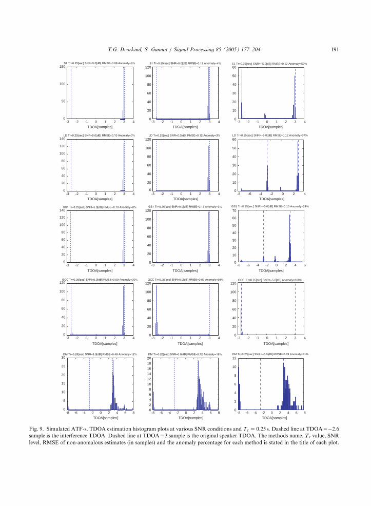
For the first static scenario we used roomdimensions of [4,7,2.75] (all dimensions are inmeters). Microphone pair is placed at [2,3.5,1.375],[1.7,3.5,1.375]. Noise source positioned at[1.5,4,2.08] and speech source is placed at[2.53,4.03,2.67]. As a result, the true TDOA forthe speech source is 3 samples, and for the noisesource is �2.6 samples. Various reverberationtimes and SNR values are tested and the ATF-sare simulated using the image method [1,33].Figs. 8 and 9 present the histogram plots of theTDOA estimation results for the various methods.If the absolute value of the TDOA estimationerror was larger than 2 samples, it was considered

9This value for a was set after applying some calculations

involving the maximal movement speed to be considered and

the asymptotic amount of data used for the TDOA estimation.

More details can be found in [16].

to be an anomaly. This threshold was determinedafter visual inspection of the TDOA estimationhistograms.As can be seen from Fig. 8, at low reverberation

conditions (T r ¼ 0:1 s) and high SNR (5 dB) allmethods perform well (this might exclude the GCCmethod that even at these mild conditions has 16%anomaly). When we test the reverberation of T r ¼

0:5 s; even in the high SNR level, the performanceof the subspace method DM and the GCC resultrapidly deteriorates. It seems that despite the useof short support analysis window P, the GCC stillsuffers from the lack of reverberant model. Thesubspace method becomes inadequate probablydue to the underestimated impulse-responselength. Possibly, this can be solved at the expenseof increased complexity, by modeling a longerimpulse responses and considering larger amountsof data. On the other hand, the simulation showsthat the proposed frequency domain methodspresent low anomaly results. As can be seen fromFig. 9, this is also the case at mid-rangereverberation T r ¼ 0:25 s and at lower SNRconditions. Note that at low SNR the decorrela-tion-based algorithms LD, GS1 outperform thestationarity-based algorithm S1. Furthermore, atlow SNR conditions the GCC is rendered useless,since it locks on the directional interference TDOAinstead of the speaker TDOA. We note that theDM method, which exploits a priori knowledge ofnoise covariance matrix, does not deteriorate atthe low SNR conditions. However, it is stilloutperformed by GS1. Evaluation of the RMSE(for the non-anomalous experiments) demon-strates that the TDOA estimates of the proposedmethods are extracted with high accuracy. TheDM method presents a higher deviation from thetrue TDOA.Next, we consider an experiment which tests the

estimation accuracy of the proposed methods atvarious SNR conditions. Specifically, we demon-strate the advantage of the decorrelation-basedmethods at low SNR conditions. Using the samegeometrical settings as described in this subsection,we have simulated the ATF-s at T r ¼ 0:1 s: Insteadof a speech signal we have filtered a whiteGaussian noise and changed its variance acrossframes. PSD estimates were obtained using large

ARTICLE IN PRESS

-3 -2 -1 0 1 2 3 40

20

40

60

80

100

120

140

TDOA[samples]

-3 -2 -1 0 1 2 3 40

10

20

30

40

50

60

70

80

90

TDOA[samples]

-3 -2 -1 0 1 2 3 40

20

40

60

80

100

120

140

TDOA[samples]

-3 -2 -1 0 1 2 3 4 5 6 70

10

20

30

40

50

60

70

80

TDOA[samples]

-3 -2 -1 0 1 2 3 40

20

40

60

80

100

120

140

TDOA[samples]

-3 -2 -1 0 1 2 3 4 5 60

10

20

30

40

50

60

70

80

90

TDOA[samples]

-3 -2 -1 0 1 2 3 40

20

40

60

80

100

120

140

TDOA[samples]

-8 -6 -4 -2 0 2 40

10

20

30

40

50

60

TDOA[samples]

-3 -2 -1 0 1 2 3 4 5 60

5

10

15

20

25

30

35

40

45

50

TDOA[samples]

-8 -6 -4 -2 0 2 4 6 80

2

4

6

8

10

12

14

TDOA[samples]

Fig. 8. Simulated ATF-s. TDOA estimation histogram plots at T r ¼ 0:1 s and T r ¼ 0:5 s: SNR= 5dB. Dashed line at TDOA=�2.6

sample is the interference TDOA. Dashed line at TDOA=3 sample is the original speaker TDOA. The methods name, T r value, SNR

level, RMSE of non-anomalous estimates (in samples) and the anomaly percentage for each method is stated in the title of each plot.


ARTICLE IN PRESS

-3 -2 -1 0 1 2 3 40

50

100

150

TDOA[samples]

-3 -2 -1 0 1 2 3 40

20

40

60

80

100

120

TDOA[samples]

-3 -2 -1 0 1 2 3 40

10

20

30

40

50

60

TDOA[samples]

-3 -2 -1 0 1 2 3 40

20

40

60

80

100

120

140

TDOA[samples]

-3 -2 -1 0 1 2 3 40

20

40

60

80

100

120

TDOA[samples]

-8 -6 -4 -2 0 2 40

10

20

30

40

50

60

TDOA[samples]

-3 -2 -1 0 1 2 3 40

20

40

60

80

100

120

140

TDOA[samples]

-3 -2 -1 0 1 2 3 40

20

40

60

80

100

120

TDOA[samples]

-8 -6 -4 -2 0 2 4 60

10

20

30

40

50

60

70

TDOA[samples]

-3 -2 -1 0 1 2 3 40

20

40

60

80

100

120

TDOA[samples]

-3 -2 -1 0 1 2 3 40

20

40

60

80

100

120

TDOA[samples]

-3 -2 -1 0 1 2 3 40

20

40

60

80

100

120

TDOA[samples]

-8 -6 -4 -2 0 2 4 6 80

5

10

15

20

25

30

TDOA[samples]

-8 -6 -4 -2 0 2 4 6 80

2

4

6

8

10

12

14

16

18

20

TDOA[samples]

-8 -6 -4 -2 0 2 4 6 80

2

4

6

8

10

12

TDOA[samples]

S1 Tr=0.25[sec] SNR=–5.0[dB] RMSE=0.12 Anomaly=52%

LD Tr=0.25[sec] SNR=–5.0[dB] RMSE=0.12 Anomaly=37%

GS1 Tr=0.25[sec] SNR=–5.0[dB] RMSE=0.15 Anomaly=24%

GCC Tr=0.25[sec] SNR=–5.0[dB] Anomaly=100%

DM Tr=0.25[sec] SNR=–5.0[dB] RMSE=0.89 Anomaly=31%

Fig. 9. Simulated ATF-s. TDOA estimation histogram plots at various SNR conditions and T r ¼ 0:25 s: Dashed line at TDOA=�2.6

sample is the interference TDOA. Dashed line at TDOA=3 sample is the original speaker TDOA. The methods name, T r value, SNR

level, RMSE of non-anomalous estimates (in samples) and the anomaly percentage for each method is stated in the title of each plot.


ARTICLE IN PRESS

-15 -10 -5 0 5 10 150

0.1

0.2

0.3

0.4

0.5

0.6

0.7

0.8

0.9

Nor

mal

ized

Err

or

SNR[dB]

S1LDGS1

Fig. 10. Estimation error of the truncated impulse response

using the proposed batch algorithms. The error is calculated

according to (27).


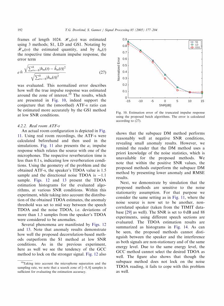
frames of length 1024. HmðoÞ was estimatedusing 3 methods; S1, LD and GS1. Notating byHmðoÞ the estimated quantity, and by hmðtÞ

the respective time domain impulse response, theerror term

e9

ffiffiffiffiffiffiffiffiffiffiffiffiffiffiffiffiffiffiffiffiffiffiffiffiffiffiffiffiffiffiffiffiffiffiffiffiffiffiffiffiffiffiffiffiP8t¼�8jhmðtÞ � hmðtÞj

2

qffiffiffiffiffiffiffiffiffiffiffiffiffiffiffiffiffiffiffiffiffiffiffiffiffiffiffiffiP8

t¼�8jhmðtÞj2

q (27)

was evaluated. This normalized error describeshow well the true impulse response was estimatedaround the zone of interest.10 The results, whichare presented in Fig. 10, indeed support theconjecture that the (smoothed) ATF-s ratio canbe estimated more accurately by the GS1 methodat low SNR conditions.

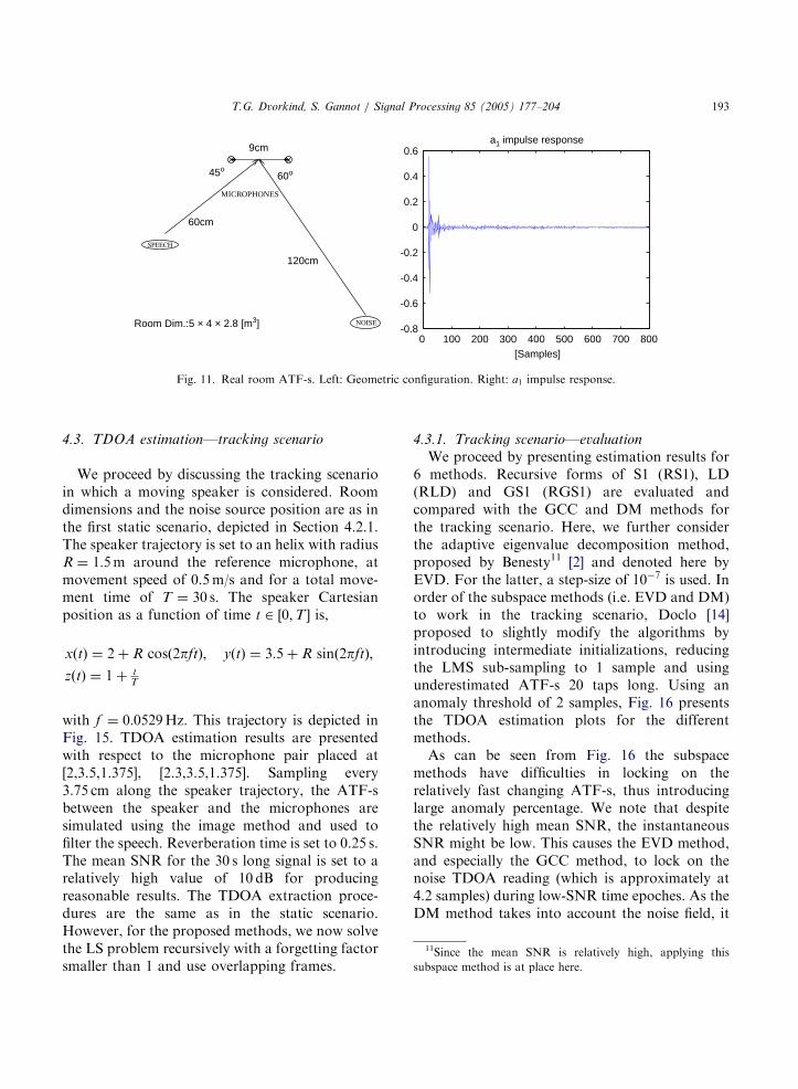
4.2.2. Real room ATF-s

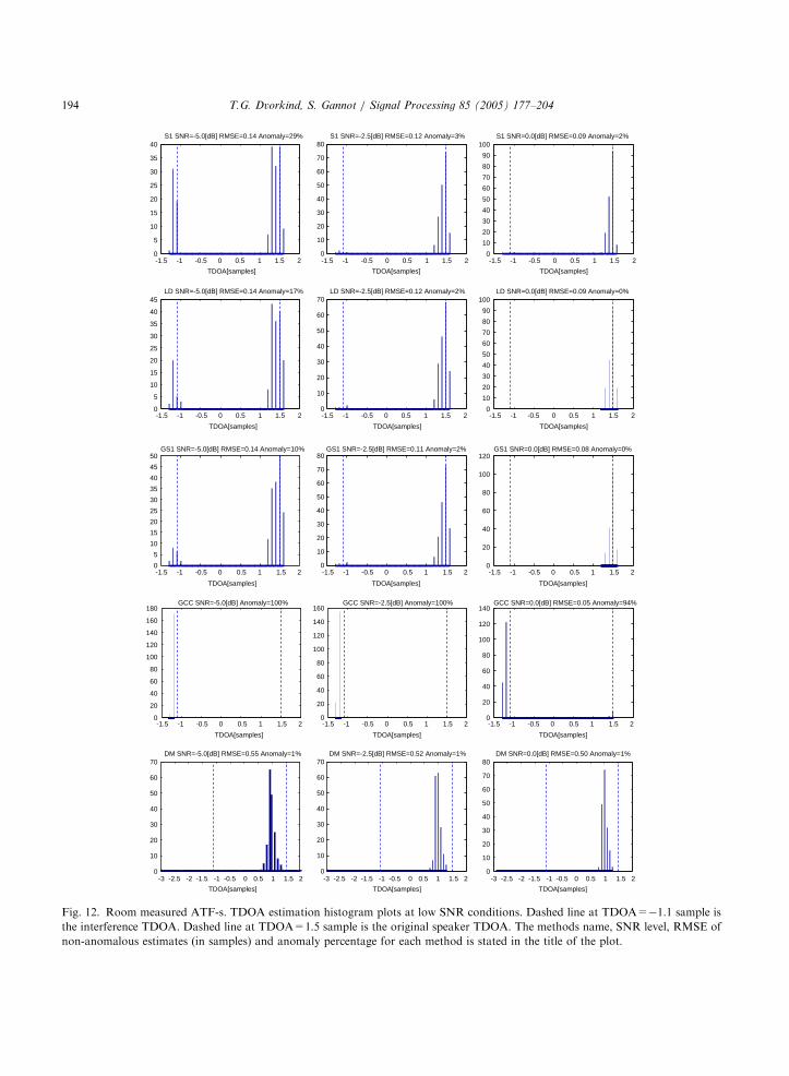
An actual room configuration is depicted in Fig.11. Using real room recordings, the ATF-s werecalculated beforehand and then used in thesimulations. Fig. 11 also presents the a1 impulseresponse which relates the source with one of themicrophones. The respective reverberation time isless than 0.1 s, indicating low reverberation condi-tions. Using the geometry of the problem and theobtained ATF-s, the speaker’s TDOA value is 1.5sample and the directional noise TDOA is �1.1sample. Figs. 12 and 13 present the TDOAestimation histograms for the evaluated algo-rithms, at various SNR conditions. Within thisexperiment, while taking into account the distribu-tion of the obtained TDOA estimates, the anomalythreshold was set to mid way between the speechTDOA and the noise TDOA, i.e. deviations ofmore than 1.3 samples from the speaker’s TDOAwere considered to be anomalies.

Several phenomena are manifested by Figs. 12and 13. Note that anomaly results demonstratehow well the proposed decorrelation-based meth-ods outperform the S1 method at low SNRconditions. As in the previous experiment,here as well we see the tendency of the GCCmethod to lock on the stronger signal. Fig. 12 also

10Taking into account the microphone separation and the

sampling rate, we note that a search zone of ½�8; 8� samples is

sufficient for evaluating the estimation accuracy.

shows that the subspace DM method performsreasonably well at negative SNR conditions,revealing small anomaly results. However, weremind the reader that the DM method uses apriori knowledge of the noise statistics, which isunavailable for the proposed methods. Wenote that within the positive SNR values, theproposed methods outperform the subspace DMmethod by presenting lower anomaly and RMSEresults.Next, we demonstrate by simulation that the

proposed methods are sensitive to the noisestationarity assumption. For that purpose weconsider the same setting as in Fig. 11, where thenoise source is now set to be another, non-correlated speaker (taken from the TIMIT data-base [29] as well). The SNR is set to 0 dB and 88experiments, using different speech sections areevaluated. The TDOA estimation results aresummarized as histograms in Fig. 14. As canbe seen, the proposed methods cannot disti-nguish between the speaker and the interferenceas both signals are non-stationary and of the sameenergy level. Due to the same energy level, theGCC method cannot select the desired TDOA aswell. The figure also shows that though thesubspace method does not lock on the noiseTDOA reading, it fails to cope with this problemas well.

ARTICLE IN PRESS

MICROPHONES

60cm

120cm

45o60o

9cm

Room Dim.:5 × 4 × 2.8 [m3]

0 100 200 300 400 500 600 700 800-0.8

-0.6

-0.4

-0.2

0

0.2

0.4

0.6a1 impulse response

[Samples]

Fig. 11. Real room ATF-s. Left: Geometric configuration. Right: a1 impulse response.

11Since the mean SNR is relatively high, applying this

subspace method is at place here.


4.3. TDOA estimation—tracking scenario

We proceed by discussing the tracking scenarioin which a moving speaker is considered. Roomdimensions and the noise source position are as inthe first static scenario, depicted in Section 4.2.1.The speaker trajectory is set to an helix with radiusR ¼ 1:5m around the reference microphone, atmovement speed of 0.5m/s and for a total move-ment time of T ¼ 30 s: The speaker Cartesianposition as a function of time t 2 ½0;T � is,

xðtÞ ¼ 2þ R cosð2pftÞ; yðtÞ ¼ 3:5þ R sinð2pftÞ;

zðtÞ ¼ 1þ tT

with f ¼ 0:0529Hz: This trajectory is depicted inFig. 15. TDOA estimation results are presentedwith respect to the microphone pair placed at[2,3.5,1.375], [2.3,3.5,1.375]. Sampling every3.75 cm along the speaker trajectory, the ATF-sbetween the speaker and the microphones aresimulated using the image method and used tofilter the speech. Reverberation time is set to 0.25 s.The mean SNR for the 30 s long signal is set to arelatively high value of 10 dB for producingreasonable results. The TDOA extraction proce-dures are the same as in the static scenario.However, for the proposed methods, we now solvethe LS problem recursively with a forgetting factorsmaller than 1 and use overlapping frames.

4.3.1. Tracking scenario—evaluation

We proceed by presenting estimation results for6 methods. Recursive forms of S1 (RS1), LD(RLD) and GS1 (RGS1) are evaluated andcompared with the GCC and DM methods forthe tracking scenario. Here, we further considerthe adaptive eigenvalue decomposition method,proposed by Benesty11 [2] and denoted here byEVD. For the latter, a step-size of 10�7 is used. Inorder of the subspace methods (i.e. EVD and DM)to work in the tracking scenario, Doclo [14]proposed to slightly modify the algorithms byintroducing intermediate initializations, reducingthe LMS sub-sampling to 1 sample and usingunderestimated ATF-s 20 taps long. Using ananomaly threshold of 2 samples, Fig. 16 presentsthe TDOA estimation plots for the differentmethods.As can be seen from Fig. 16 the subspace

methods have difficulties in locking on therelatively fast changing ATF-s, thus introducinglarge anomaly percentage. We note that despitethe relatively high mean SNR, the instantaneousSNR might be low. This causes the EVD method,and especially the GCC method, to lock on thenoise TDOA reading (which is approximately at4.2 samples) during low-SNR time epoches. As theDM method takes into account the noise field, it

ARTICLE IN PRESS

0

5

10

15

20

25

30

35

40S1 SNR=-5.0[dB] RMSE=0.14 Anomaly=29%

TDOA[samples]

0

10

20

30

40

50

60

70

80S1 SNR=-2.5[dB] RMSE=0.12 Anomaly=3%

TDOA[samples]

0

10

20

30

40

50

60

70

80

90

100S1 SNR=0.0[dB] RMSE=0.09 Anomaly=2%

TDOA[samples]

0

5

10

15

20

25

30

35

40

45LD SNR=-5.0[dB] RMSE=0.14 Anomaly=17%

TDOA[samples]

0

10

20

30

40

50

60

70LD SNR=-2.5[dB] RMSE=0.12 Anomaly=2%

TDOA[samples]

0

10

20

30

40

50

60

70

80

90

100LD SNR=0.0[dB] RMSE=0.09 Anomaly=0%

TDOA[samples]

0

5

10

15

20

25

30

35

40

45

50GS1 SNR=-5.0[dB] RMSE=0.14 Anomaly=10%

TDOA[samples]

0

10

20

30

40

50

60

70

80GS1 SNR=-2.5[dB] RMSE=0.11 Anomaly=2%

TDOA[samples]

0

20

40

60

80

100

120GS1 SNR=0.0[dB] RMSE=0.08 Anomaly=0%

TDOA[samples]

-1.5 -1 -0.5 0 0.5 1 1.5 2

-1.5 -1 -0.5 0 0.5 1 1.5 2

-1.5 -1 -0.5 0 0.5 1 1.5 2

-1.5 -1 -0.5 0 0.5 1 1.5 2 -1.5 -1 -0.5 0 0.5 1 1.5 2 -1.5 -1 -0.5 0 0.5 1 1.5 2

-1.5 -1 -0.5 0 0.5 1 1.5 2 -1.5 -1 -0.5 0 0.5 1 1.5 2

-1.5 -1 -0.5 0 0.5 1 1.5 2 -1.5 -1 -0.5 0 0.5 1 1.5 2

-1.5 -1 -0.5 0 0.5 1 1.5 2 -1.5 -1 -0.5 0 0.5 1 1.5 20

20

40

60

80

100

120

140

160

180GCC SNR=-5.0[dB] Anomaly=100%

TDOA[samples]

0

20

40

60

80

100

120

140

160GCC SNR=-2.5[dB] Anomaly=100%

TDOA[samples]

0

20

40

60

80

100

120

140GCC SNR=0.0[dB] RMSE=0.05 Anomaly=94%

TDOA[samples]

-3 -2.5 -2 -1.5 -1 -0.5 0 0.5 1 1.5 2 -3 -2.5 -2 -1.5 -1 -0.5 0 0.5 1 1.5 2 -3 -2.5 -2 -1.5 -1 -0.5 0 0.5 1 1.5 20

10

20

30

40

50

60

70DM SNR=-5.0[dB] RMSE=0.55 Anomaly=1%

TDOA[samples]

0

10

20

30

40

50

60

70DM SNR=-2.5[dB] RMSE=0.52 Anomaly=1%

TDOA[samples]

0

10

20

30

40

50

60

70

80DM SNR=0.0[dB] RMSE=0.50 Anomaly=1%

TDOA[samples]

Fig. 12. Room measured ATF-s. TDOA estimation histogram plots at low SNR conditions. Dashed line at TDOA=�1.1 sample is

the interference TDOA. Dashed line at TDOA=1.5 sample is the original speaker TDOA. The methods name, SNR level, RMSE of

non-anomalous estimates (in samples) and anomaly percentage for each method is stated in the title of the plot.


ARTICLE IN PRESS

-1.5 -1 -0.5 0 0.5 1 1.5 2 -1.5 -1 -0.5 0 0.5 1 1.5 2

-1.5 -1 -0.5 0 0.5 1 1.5 2 -1.5 -1 -0.5 0 0.5 1 1.5 2

-1.5 -1 -0.5 0 0.5 1 1.5 2 -1.5 -1 -0.5 0 0.5 1 1.5 2

-1.5 -1 -0.5 0 0.5 1 1.5 2 -1.5 -1 -0.5 0 0.5 1 1.5 2

0

20

40

60

80

100

120


TDOA[samples]

0

20

40

60

80

100

120

140


TDOA[samples]

0

20

40

60

80

100

120


TDOA[samples]

0

20

40

60

80

100

120

140


TDOA[samples]

0

50

100


TDOA[samples]

0

20

40

60

80

100

120

140

160


TDOA[samples]

0

10

20

30

40

50

60

70


TDOA[samples]

0

20

40

60

80

100


TDOA[samples]

-3 -2.5 -2 -1.5 -1 0.5 0 0.5 1 1.5 20

10

20

30

40

50

60

70

80


TDOA[samples]

-3 -2.5 -2 -1.5 -1 0.5 0 0.5 1 1.5 2

TDOA[samples]

0

10

20

30

40

50

60

70


Fig. 13. Room measured ATF-s. TDOA estimation histogram plots at high SNR conditions. Dashed line at TDOA=�1.1 sample is

the interference TDOA. Dashed line at TDOA=1.5 sample is the original speaker TDOA. The methods name, SNR level, RMSE of

non-anomalous estimates (in samples) and anomaly percentage for each method is stated in the title of the plot.


ARTICLE IN PRESS

-1.5 -1 -0.5 0 0.5 1 1.5 2

-1.5 -1 -0.5 0 0.5 1 1.5 2

-1.5 -1 -0.5 0 0.5 1 1.5 2 -1.5 -1 -0.5 0 0.5 1 1.5 20

5

10

15

20

25

30

35S1

TDOA[samples]

0

5

10

15

20

25

30

35LD

TDOA[samples]

0

5

10

15

20

25

30GS1

TDOA[samples]

0

5

10

15

20

25

30

35GCC

TDOA[samples]

-3 -2.5 -2 -1.5 -1 -0.5 0 0.5 1 1.5 20

1

2

3

4

5

6

7

8

9DM

TDOA[samples]

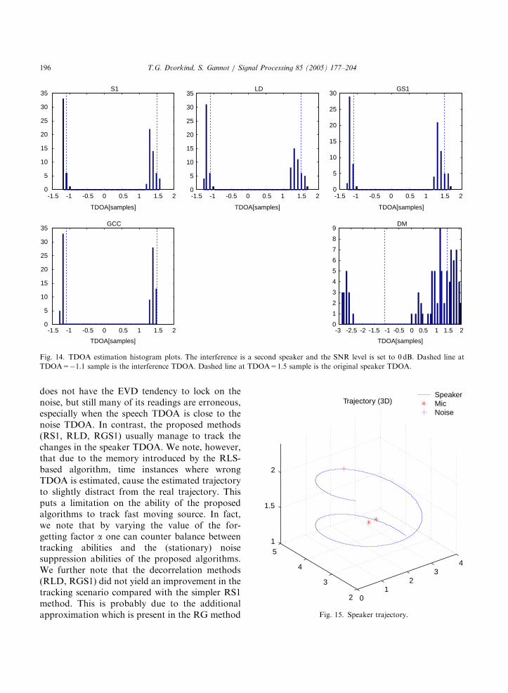
Fig. 14. TDOA estimation histogram plots. The interference is a second speaker and the SNR level is set to 0 dB. Dashed line at

TDOA=�1.1 sample is the interference TDOA. Dashed line at TDOA=1.5 sample is the original speaker TDOA.

01

23

4

2

3

4

51

1.5

2

Trajectory (3D)SpeakerMicNoise

Fig. 15. Speaker trajectory.


does not have the EVD tendency to lock on thenoise, but still many of its readings are erroneous,especially when the speech TDOA is close to thenoise TDOA. In contrast, the proposed methods(RS1, RLD, RGS1) usually manage to track thechanges in the speaker TDOA. We note, however,that due to the memory introduced by the RLS-based algorithm, time instances where wrongTDOA is estimated, cause the estimated trajectoryto slightly distract from the real trajectory. Thisputs a limitation on the ability of the proposedalgorithms to track fast moving source. In fact,we note that by varying the value of the for-getting factor a one can counter balance betweentracking abilities and the (stationary) noisesuppression abilities of the proposed algorithms.We further note that the decorrelation methods(RLD, RGS1) did not yield an improvement in thetracking scenario compared with the simpler RS1method. This is probably due to the additionalapproximation which is present in the RG method

ARTICLE IN PRESS

0 5 10 15 20 25 30-8

-6

-4

-2

0

2

4

6

8

-8

-6

-4

-2

0

2

4

6

8

-8

-6

-4

-2

0

2

4

6

8

Time[sec]

TD

OA

[sam

ple]

RS1(Bias=-0.15[sample], RMSE=0.58[sample], Anomaly=4%)

0 5 10 15 20 25 30-8

-6

-4

-2

0

2

4

6

8

Time[sec]

TD

OA

[sam

ple]

RLD(Bias=-0.13[sample], RMSE=0.58[sample], Anomaly=6%)

0 5 10 15 20 25 30

Time[sec]

TD

OA

[sam

ple]

RGS1(Bias=-0.16[sample], RMSE=0.60[sample], Anomaly=9%)

0 5 10 15 20 25 30-8

-6

-4

-2

0

2

4

6

8

Time[sec]

TD

OA

[sam

ple]

GCC(Bias=-0.09[sample], RMSE=0.46[sample], Anomaly=31%)

0 5 10 15 20 25 30

Time[sec]

TD

OA

[sam

ple]

DM

(Bias=-0.17[sample], RMSE=0.63[sample], Anomaly=37%)

0 5 10 15 20 25 30-8

-6

-4

-2

0

2

4

6

8

Time[sec]

TD

OA

[sam

ple]

EVD


Fig. 16. Moving source scenario, TDOA estimation results. Solid line: True TDOA. Dots: Estimation results. The method’s name, its

bias, RMSE and anomaly results are presented in the title of each plot.


and not suitable for this relatively fast changingscenario.

It is interesting to investigate the performance ofthe suggested algorithms in a stationary diffusednoise field as well. Diffused noise field is

typical to car environments. The respectivecoherence function between two sensors isgiven by gðoÞ ¼ ðFzizj

ðoÞ=ffiffiffiffiffiffiffiffiffiffiffiffiffiffiffiffiffiffiffiffiffiffiffiffiffiffiffiffiffiffiffiFzizi

ðoÞFzjzjðoÞ

pÞ ¼

ðsinðoðd=cÞÞ=oðd=cÞÞ (where d is the micro-phone separation distance and c is the sound

ARTICLE IN PRESS

0 500 1000 1500 2000 2500 3000 3500 40000

0.1

0.2

0.3

0.4

0.5

0.6

0.7

0.8

0.9

1

Freq.[Hz]

Diffused noise spectral coherence

γ

Fig. 17. Coherence function for the diffused noise.

0 5 10 15 20 25 30-8

-6

-4

-2

0

2

4

6

8

Time[sec]

TD

OA

[sam

ple]


TD

OA

[sam

ple]

0 5 10 15 20 25 30-8

-6

-4

-2

0

2

4

6

8

Time[sec]

TD

OA

[sam

ple]

RGS1(Bias=-0.17[sample], RMSE=0.73[sample], Anomaly=11%)

TD

OA

[sam

ple]

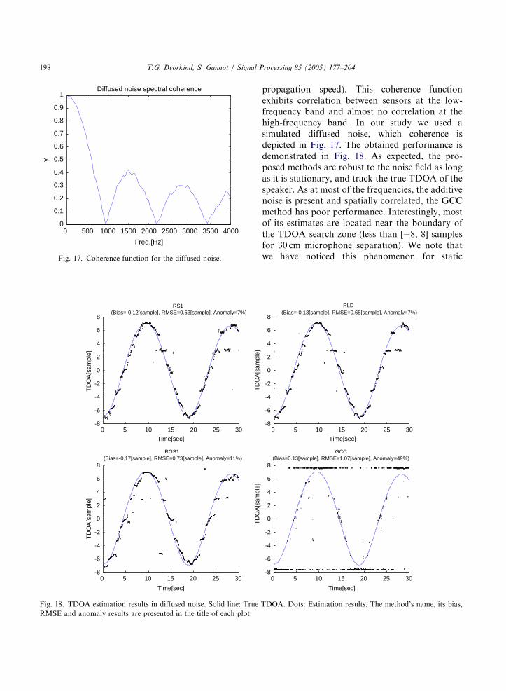
Fig. 18. TDOA estimation results in diffused noise. Solid line: True

RMSE and anomaly results are presented in the title of each plot.


propagation speed). This coherence functionexhibits correlation between sensors at the low-frequency band and almost no correlation at thehigh-frequency band. In our study we used asimulated diffused noise, which coherence isdepicted in Fig. 17. The obtained performance isdemonstrated in Fig. 18. As expected, the pro-posed methods are robust to the noise field as longas it is stationary, and track the true TDOA of thespeaker. As at most of the frequencies, the additivenoise is present and spatially correlated, the GCCmethod has poor performance. Interestingly, mostof its estimates are located near the boundary ofthe TDOA search zone (less than [�8, 8] samplesfor 30 cm microphone separation). We note thatwe have noticed this phenomenon for static

0 5 10 15 20 25 30-8

-6

-4

-2

0

2

4

6

8

Time[sec]

RLD(Bias=-0.13[sample], RMSE=0.65[sample], Anomaly=7%)

0 5 10 15 20 25 30-8

-6

-4

-2

0

2

4

6

8

Time[sec]

GCC(Bias=0.13[sample], RMSE=1.07[sample], Anomaly=49%)

TDOA. Dots: Estimation results. The method’s name, its bias,

ARTICLE IN PRESS


scenarios as well, and for different settings of thesearch zone.

As the simpler RS1 method performed better inthe tracking scenarios only the latter is presentedin the evaluation to follow.

4.3.2. Switching scenario—evaluation

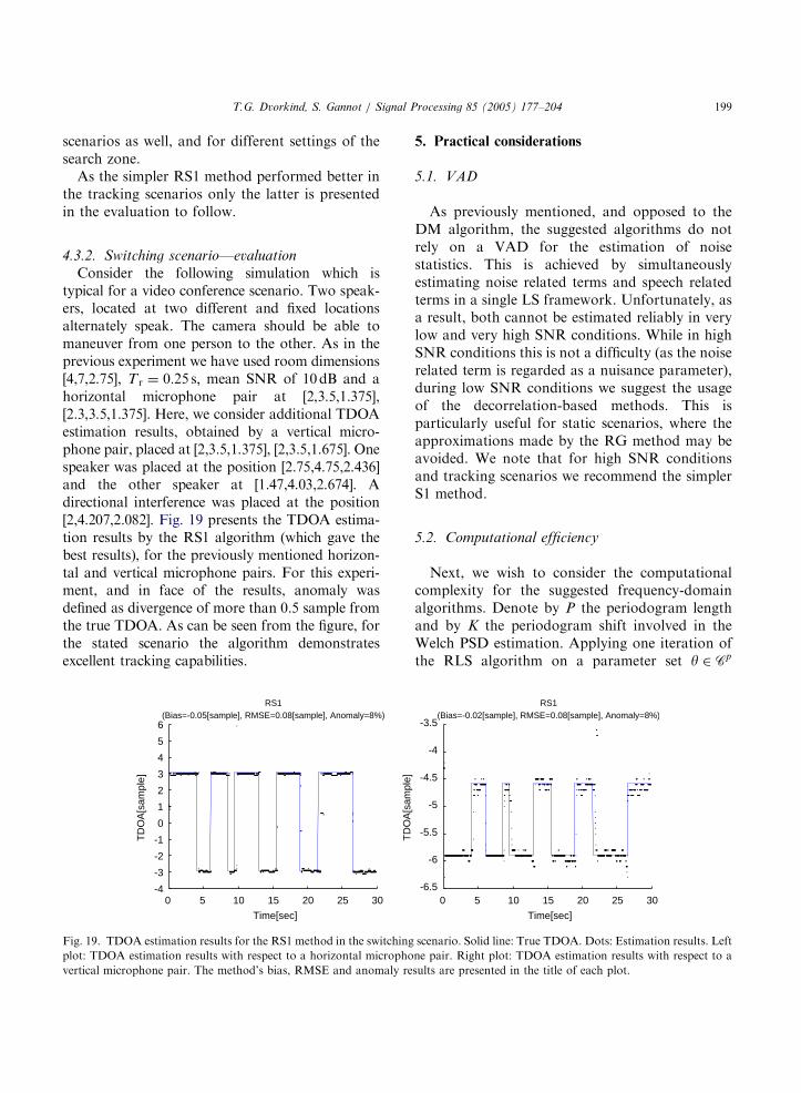
Consider the following simulation which istypical for a video conference scenario. Two speak-ers, located at two different and fixed locationsalternately speak. The camera should be able tomaneuver from one person to the other. As in theprevious experiment we have used room dimensions[4,7,2.75], T r ¼ 0:25 s; mean SNR of 10dB and ahorizontal microphone pair at [2,3.5,1.375],[2.3,3.5,1.375]. Here, we consider additional TDOAestimation results, obtained by a vertical micro-phone pair, placed at [2,3.5,1.375], [2,3.5,1.675]. Onespeaker was placed at the position [2.75,4.75,2.436]and the other speaker at [1.47,4.03,2.674]. Adirectional interference was placed at the position[2,4.207,2.082]. Fig. 19 presents the TDOA estima-tion results by the RS1 algorithm (which gave thebest results), for the previously mentioned horizon-tal and vertical microphone pairs. For this experi-ment, and in face of the results, anomaly wasdefined as divergence of more than 0.5 sample fromthe true TDOA. As can be seen from the figure, forthe stated scenario the algorithm demonstratesexcellent tracking capabilities.

0 5 10 15 20 25 30-4

-3

-2

-1

0

1

2

3

4

5

6

Time[sec]

TD

OA

[sam

ple]


TD

OA

[sam

ple]

RS1

Fig. 19. TDOA estimation results for the RS1 method in the switching

plot: TDOA estimation results with respect to a horizontal micropho

vertical microphone pair. The method’s bias, RMSE and anomaly re

5. Practical considerations

5.1. VAD

As previously mentioned, and opposed to theDM algorithm, the suggested algorithms do notrely on a VAD for the estimation of noisestatistics. This is achieved by simultaneouslyestimating noise related terms and speech relatedterms in a single LS framework. Unfortunately, asa result, both cannot be estimated reliably in verylow and very high SNR conditions. While in highSNR conditions this is not a difficulty (as the noiserelated term is regarded as a nuisance parameter),during low SNR conditions we suggest the usageof the decorrelation-based methods. This isparticularly useful for static scenarios, where theapproximations made by the RG method may beavoided. We note that for high SNR conditionsand tracking scenarios we recommend the simplerS1 method.

5.2. Computational efficiency

Next, we wish to consider the computationalcomplexity for the suggested frequency-domainalgorithms. Denote by P the periodogram lengthand by K the periodogram shift involved in theWelch PSD estimation. Applying one iteration ofthe RLS algorithm on a parameter set y 2 Cp

0 5 10 15 20 25 30-6.5

-6

-5.5

-5

-4.5

-4

-3.5

Time[sec]


scenario. Solid line: True TDOA. Dots: Estimation results. Left

ne pair. Right plot: TDOA estimation results with respect to a

sults are presented in the title of each plot.

ARTICLE IN PRESS


involves 10p2 þ 12p real multiplications and onecomplex division. Noting that RLS iteration isperformed in each frequency bin and that there areP=2 frequencies to evaluate, the total number ofreal multiplications performed by the RLS isPð10p2 þ 12pÞ=2: The suggested frequency domainalgorithms further involve one IFFT operationand interpolation. Assuming that the interpolationis conducted for S samples12 with a 1/10 sampleresolution, the last stage involves approximately2P log2 P þ 10S2 real multiplications. Consider forexample the RS1 algorithm. Cross-PSD Fzmz1 ðoÞand auto-PSD Fz1z1ðoÞ can be compactly evalu-ated for every new K samples using

2 P þ 2P log2P þ3P

2

�¼ 2Pð2:5þ 2 log2 PÞ

real multiplications. Considering the RLS itera-tions and the time domain post-processing, thecomputational burden per sample is

2Pð2:5þ 2 log2 PÞ þ Pð10p2 þ 12pÞ=2þ 2P log2 P þ 10S2

K

real multiplications. For RS1 algorithm p ¼ 2:Assuming that S ¼ 17; P ¼ 256; K ¼ 128 thisyields approximately 193 multiplications per sam-ple. We note that this burden is higher than theone imposed by the simpler GCC method, but it isusually much lower than the burden imposed bythe subspace methods.

6. Summary

In this work novel TDOA estimation algo-rithms, based on the ATF-s ratio HmðoÞ forTDOA extraction, were presented. Speech quasi-stationarity, noise stationarity and the fact thatthere is no correlation between the speech and thenoise were used for HmðoÞ estimation. Noisestationarity was employed for resolving frequencypermutation ambiguity, inherent to the frequencydomain decorrelation criterion. Simulation resultsrevealed superiority over the classical generalized

cross correlation (GCC) method and the recently

12The region of interest for conducting the interpolation is

bounded by the microphone pair separation.

proposed subspace method. Preliminary experi-ments showed that the use of short supportanalysis window can improve the robustness ofthe GCC algorithm to reverberation. Computa-tional considerations, presented in Section 5,revealed that the suggested frequency domainmethods result in relatively low computationalcosts. Special care was given to recursive imple-mentation which is applicable for the trackingscenario. This resulted in a general formulation,notated by recursive Gauss, for recursive solutionof a nonlinear equation set.

Acknowledgements

We would like to thank Dr. Simon Doclo fromK.U. Leuven, Belgium for generously making hissimulation code available for us and for hisvaluable remarks. We also would like to thankthe anonymous reviewers for their thorough workand valuable comments.

Appendix A. The Gauss method

Let y 2 Cp be an unknown p � 1 parametervector, which is measured through K nonlinearequations h resulting a measurement vector v

hðyÞ ¼ v :

Expansion of hðyÞ around yð0Þ; using first-orderapproximation becomes

hðyÞ � hðyð0ÞÞ þHðyð0ÞÞðy�yð0ÞÞ (A.1)

with H being a K � p gradient matrix such thatHk;q ¼ @hk=@yq: Thus

Hðyð0ÞÞ y � v� hðyð0ÞÞ þHðyð0ÞÞyð0Þ:

When K4p; this is an overdetermined set whichcan be solved in the LS sense, resulting theiterative algorithm

yðlþ1Þ¼ ðHðyðlÞÞyHðyðlÞÞÞ�1HðyðlÞÞyðv� hðyðlÞÞ

þHðyðlÞÞyðlÞÞ ðA:2Þ

ARTICLE IN PRESS


which is equivalent to

yðlþ1Þ¼ yðlÞ þ ðHðyðlÞÞyHðyðlÞÞÞ�1HðyðlÞÞy

�ðv� hðyðlÞÞÞ: ðA:3Þ

Appendix B. Recursive least squares

Sequential solution to the linear LS problemA y � y can be obtained on a frame-by-framebasis, using the recursive least squares (RLS)algorithm. Consider a weighted LS (WLS) pro-blem for estimating the parameter set y 2 Cp basedon N equations:

yðNÞ ¼ arg miny

ðA1:N y�y1:N

ÞyW1:NðA1:N y�y

1:NÞ

(B.1)

with

W1:N ¼

aN�1 0 . . . 0

0 . .. ..

.

..

.a 0

0 . . . 0 1

2666664

3777775 (B.2)

a diagonal N � N weight matrix, with the nthelement along the diagonal set to aN�n: a is theforgetting factor, 0oap1: A1:N stands for an N �

p matrix and y1:N

is an N � 1 measurement vector

A1:N9

ay

1

..

.

ay

N

2664

3775; y

1:N9

y1

..

.

yN

2664

3775

with an; n ¼ 1; . . . ;N a p � 1 vector. Then, therecursive solution to (B.1) takes the known form(see for example [24,26]):

Kn ¼Pn�1an

aþ aynPn�1an

;

yðnÞ ¼ yðn � 1Þ þ Knðyn � aynyðn � 1ÞÞ;

Pn ¼Xn

t¼1

an�tatayt

!�1

¼ ðPn�1 � KnaynðPn�1Þ

1

a; ðB:3Þ

where Pn is the weighted inverse. To avoid directcalculation of the initial inverse P0; a commonapproach is to use the diagonal initialization P0 ¼

bI with bb1:

Appendix C. Recursive nonlinear least squares

In this appendix, a method is derived forrecursive estimate of a nonlinear LS problem.The method first resolves the nonlinearities byfirst-order approximation, as in the Gauss method.Then, by proper approximation, a recursion isderived. We denote this recursive procedure byRG.Consider a nonlinear equation set for a p � 1

parameter vector y 2 Cp

h1:NðyÞ ¼ d1:N

with

h1:NðyÞ9

h1ðyÞ

..

.

hNðyÞ

2664

3775; d1:N9

d1

..

.

dN

2664

3775:

Applying first-order approximation around aninitial guess yð0Þ (as with the Gauss method) weobtain

h1:Nðyð0ÞÞ þH1:Nðy

ð0ÞÞðy�yð0ÞÞ � d1:N ; (C.1)

where H1:N is the N � p gradient matrix

H1:N ðyÞ9

H1ðyÞ

..

.

HN ðyÞ

2664

3775

with HnðyÞ ¼ ryhnðyÞ the gradient row vector ofhnðyÞ: According to the Gauss method, theiterative LS solution to the linearized set (C.1) is

yðlþ1Þ¼ ðH1:N ðy

ðlÞÞyH1:N ðy

ðlÞÞÞ�1H1:Nðy

ðlÞÞy

�ðd1:N � h1:NðyðlÞÞ þH1:Nðy

ðlÞÞyðlÞÞ;

where the superscript denotes the iteration num-ber. Consider the next measurement hNþ1ðyÞ ¼dNþ1 available at time instance N þ 1: In order toestimate y we will use all the available measure-ments simultaneously. Though we could approx-imate all N þ 1 equations at the current estimate

ARTICLE IN PRESS


yðlþ1Þ; we will do so only for the new equation.Namely, instead of minimizing in the LS sense thefollowing residual norm

miny

kd1:Nþ1 � ðh1:Nþ1ðyðlþ1Þ

Þ

þH1:Nþ1ðyðlþ1Þ

Þðy�yðlþ1ÞÞÞk

we will minimize

miny

d1:N � ðh1:N ðyðlÞÞ þH1:Nðy

ðlÞÞðy�yðlÞÞÞ

dNþ1 � ðhNþ1ðyðlþ1Þ

Þ þHNþ1ðyðlþ1Þ

Þðy�yðlþ1ÞÞÞ

��

��:

The reason for this approximation is to keep pastsolutions intact, i.e. when new equation becomesavailable there is no need to update past solutionsbased on the new equation, thus, enabling arecursive solution to be derived. Now, usingstochastic approximation, i.e. replacing the itera-tion index by the time index, a sequentialalgorithm is obtained. To summarize the proce-dure, an estimate for y at the current time instancen (denoted by yðnÞ) is obtained by solving thefollowing LS problem sequentially using the RLSprocedure

yðnÞ ¼ arg miny

H1ðyð0ÞÞ

..

.

Hnðyðn � 1ÞÞ

2664

3775 y�y

1:n

��

��

��

��; (C.2)

where

y1:n9

d1 � h1ðyð0ÞÞ þ H1ðyð0ÞÞyð0Þ

..

.

dn � hnðyðn � 1ÞÞ þ Hnðyðn � 1ÞÞyðn � 1Þ

2664

3775

with yð0Þ the initial estimate for the parameter set.Recalling that in tracking problems the parameterset y might slowly vary with time, a commonpractice is to apply the RLS algorithm with adiagonal weight matrix, as depicted in (B.2).

We also note that the resulting algorithm can beviewed as a special case of the extended Kalman

filter. The detailed derivation is out of the scope ofthis work and can be found in [18].

Appendix D. Recursive least squares for multiple

readings

Assume a scenario in which for each timeinstance we have K scalar measurements zt 2 CK

related to an unknown p � 1 parameter vector y 2

Cp by a linear K � p transformation Ht

zt � Ht y :

The approximation is due to the fact that themeasurements are noisy, or due to slight modelingerrors. N time instances can be augmented to amatrix form z1:N � H1:N y where

z1:N9

z1

..

.

zN

2664

3775; H1:N9

H1

..

.

HN

2664

3775:

The weighted LS (WLS) solution for y; using non-negative weight matrix W1:N (of size KN � KN) is

y ¼ ðHy

1:NW1:NH1:N Þ�1H

y

1:NW1:Nz1:N : (D.1)

Our goal is to evaluate (D.1) recursively. If theparameters slowly change, a common approach isto apply a diagonal weight matrix W1:N withpowers of a forgetting factor 0oap1 along itsdiagonal. Note, that for measurements associatedwith the same time instance, we wish to apply thesame factor, since equations of the same timeinstance have equal importance. Such weightmatrix can be represented recursively as

W1:N ¼aW1:N�1 0

0y I

� �; W1:1 ¼ I;

where I and 0 stand for the identity and zeromatrices of sizes K � K and ðN � 1ÞK � K ;respectively. Though it might seem that in orderto derive a recursive solution for (D.1) a K � K

matrix inversion should be made in each RLSiteration, in practice the complexity can be furtherreduced. This is obtained by applying the well-known RLS algorithm with a minor twist. Con-sider a single equation which is updated into therecursion. We must check if this new equationbelongs to the next time instance. If so, a memoryfactor ap1 is applied. If this is not the case and weare evaluating one of the K equations of thecurrent time instance, a memory factor of 1 is

ARTICLE IN PRESS


used. Thus, in order to derive a recursion, wherethe update stage considers a single equation, theforgetting factor should vary. Notating thetime instance by n and the sequential number ofthe equation by nK þ k (where k 2 f1; . . . ;Kg) theforgetting factor becomes

forgetting factor ¼a; k ¼ 1;

1 otherwise:

�

References

[1] J.B. Allen, D.A. Berkley, Image method for efficiently

simulating small-room acoustics, J. Acoust. Soc. Am. 65

(4) (1979) 943–950.

[2] J. Benesty, Adaptive eigenvalue decomposition algorithm

for passive acoustic source localization, Acoust. Soc. Am.

107 (1) (2000) 384–391.

[3] S.T. Birchfield, D.K. Gillmor, Fast Bayesian acoustic

localization, Proceedings of the IEEE International Con-

ference on Acoustics, Speech, and Signal Processing, vol. 2,

Orlando, Florida, May 2002, pp. 1793–1796.

[4] M.S. Brandstein, J.E. Adcock, H.F. Silverman, A closed-

form location estimator for use with room environment

microphone arrays, IEEE Trans. Speech Audio Process. 5

(1) (1997) 45–50.

[5] M. Brandstein, H. Silverman, A robust method for speech

signal time-delay estimation in reverberant rooms, in:

Proceedings of the IEEE International Conference on

Acoustics, Speech and Signal Processing, 1997, pp.

375–378.

[6] M. Cetin, D.M. Malioutov, A.S. Willsky, A variational

technique for source localization based on a sparse signal

reconstruction perspective, Proceedings of the IEEE

International Conference on Acoustics, Speech, and

Signal Processing, vol. 3, Orlando, Florida, May 2002,

pp. 2965–2968.

[7] B. Champagne, S. Bedard, A. Stephenne, Performance of

time-delay estimation in the presence of room reverbera-

tion, IEEE Trans. Acoust. Speech Signal Process. 4 (2)

(1996) 148–152.

[8] C. Chen, R. Hudson, Maximum-likelihood acoustic source

localization: experimental results, Proceedings of the IEEE

International Conference on Acoustics, Speech, and Signal

Processing, vol. 3, Orlando, Florida, May 2002, pp.

2949–2952.

[9] C. Chen, R. Hudson, K. Yao, Maximum-likelihood source

localization and unknown sensor location estimation for

wideband signals in the near-field, IEEE Trans. Signal

Process. 50 (8) (2002) 1843–1854.

[10] H.H. Chiang, C.L. Nikias, A new method for adaptive

time-delay estimation for non-Gaussian signals, IEEE

Trans. Acoust. Speech Signal Process. 38 (2) (1990)

209–219.

[11] J. DiBiase, H. Silverman, M. Brandstein, Robust Locali-

zation in Reverberant Rooms, Springer, Berlin, 2001.

[12] E.D. DiClaudio, R. Parisi, G. Orlandi, Multi-source

localization in reverberant environments by root-music

and clustering, in: ICASSP-2000, 2000, pp. 921–924.

[13] S. Doclo, Multi-microphone noise reduction and derever-

beration techniques for speech applications, Ph.D. Thesis,

Katholieke Universiteit Leuven, May 2003.

[14] S. Doclo, Modification of robust time-delay estimation in

highly adverse acoustic environments for tracking scenar-

ios, Private communication, August 2003.

[15] S. Doclo, M. Moonen, Robust adaptive time delay

estimation for speaker localisation in noisy and reverber-

ant acoustic environments, EURASIP J. Appl. Signal

Process. 2003 (11) (2003) 1110–1124.

[16] T.G. Dvorkind, Speaker localization in a reverberant and

noisy environment, Master’s Thesis, Technion—Israel

Institute of Technology, December 2003.

[17] T. Dvorkind, S. Gannot, Speaker localization in a

reverberant environment, IEEE Proceedings, The 22nd

Convention of Electrical and Electronics Engineers in

Israel, 2002, pp. 7–9.

[18] T. Dvorkind, S. Gannot, Speaker localization exploiting

spatial-temporal information, in: International Workshop

on Acoustic Echo and Noise Control, Kyoto, Japan, 2003,

pp. 295–298.

[19] T. Dvorkind, S. Gannot, Approaches for time difference of

arrival estimation in a noisy and reverberant environment,

in: International Workshop on Acoustic Echo and Noise

Control, Kyoto, Japan, 2003, pp. 215–218.

[20] D.R. Fischell, C.H. Coker, A speech direction finder, in:

Proceedings of the 1984 IEEE International Conference on

Acoustics, Speech and Signal Processing (ICASSP-84),

1984, pp. 19.8.1–19.8.4.

[21] J. Fuchs, On the application of the global matched filter to

DOA estimation with uniform circular arrays, IEEE

Trans. Signal Process. 49 (4) (2001) 702–709.

[22] S. Gannot, D. Burshtein, E. Weinstein, Signal enhance-

ment using beamforming and non-stationarity with appli-

cation to speech, IEEE Trans. Signal Process. 49 (8) (2001)

1614–1626.

[23] S. Gannot, A. Yeredor, Noise cancellation with static mixtures

of a nonstationary signal and stationary noise, EURASIP J.

Appl. Signal Process. 2002 (12) (2002) 1460–1472.

[24] S. Haykin, Adaptive Filter Theory, third ed., Prentice-

Hall, Englewood Cliffs, NJ, 1996.

[25] Y. Huang, J. Benesty, G.W. Elko, R.M. Mersereau, Real-

time passive source localization: a practical linear-correc-

tion least-squares approach, IEEE Trans. Speech Audio

Process. 9 (8) (2001) 943–956.

[26] T. Kailath, A. Sayed, B. Hassibi, Linear Estimation,

Prentice-Hall, Englewood Cliffs, NJ, 2000.

[27] C. Knapp, G. Carter, The generalized correlation method

for estimation of time delay, IEEE Trans. Acoust. Speech

Signal Process. 24 (4) (1976) 320–327.

[28] H. Kurtuff, Room Acoustics, third ed., Elsevier, London,

UK, 1991.

ARTICLE IN PRESS


[29] National Institute of Standards and Technology, The

DARPA TIMIT acoustic-phonetic continuous speech

corpus, CD-ROM NIST Speech Disc 1-1.1, October 1991.

[30] C. Nikias, R. Pan, Time delay estimation in unknown

Gaussian spatially correlated noise, IEEE Trans. Acoust.

Speech Signal Process. 36 (11) (1988) 1706–1714.

[31] T. Nishiura, S. Nakamura, K. Shikano, Talker localization

in a real acoustic environment based on DOA estimation

and statistical sound source identification, Proceedings of

the IEEE International Conference on Acoustics, Speech,

and Signal Processing, vol. 1, Orlando, Florida, May 2002,

pp. 893–896.

[32] L. Parra, C. Spence, Convolutive blind separation of non-

stationary sources, IEEE Trans. Speech Audio Process. 8

(3) (2000) 320–327.

[33] P. Peterson, Simulating the response of multiple micro-

phones to a single acoustic source in a reverberant room, J.

Acoust. Soc. Am. 76 (5) (1986) 1527–1529.

[34] K. Rahbar, J.P. Reilly, Blind source separation for MIMO

convolutive mixtures, in: Third International Conference

on ICA and BSS, San Diego, California, USA, 2001,

pp. 242–247.

[35] R. Schmidt, Multiple emitter location and signal para-

meter estimation, IEEE Trans. Antennas and Propagation

AP-34 (3) (1986) 276–280.

[36] D. Schobben, P. Sommen, A frequency domain blind

signal separation method based on decorrelation, IEEE

Trans. Signal Process. 50 (8) (2002) 1855–1865.

[37] O. Shalvi, E. Weinstein, System identification using

nonstationary signals, IEEE Trans. Signal Process. 44 (8)

(1996) 2055–2063.

[38] A. Stephene, B. Champagne, A new cepstral prefiltering

technique for estimating time delay under reverberant

conditions, Signal Process. 59 (1997) 253–266.

[39] A. Varga, H.J.M. Steeneken, Assessment for automatic

speech recognition: II. NOISEX-92: a database and

an experiment to study the effect of additive noise on

speech recognition systems, Speech Commun. 12 (1993)

247–251.

[40] H. Wang, M. Kaveh, Coherent signal-subspace processing

for the detection and estimation of angles of arrival of

multiple wide-band sources, IEEE Trans. Acoust. Speech

Signal Process. 33 (4) (1985) 823–831.

[41] E. Weinstein, M. Feder, A.V. Oppenheim, Multi-channel

signal separation by decorrelation, IEEE Trans. Speech

Audio Process. 1 (4) (1993) 405–413.

[42] P.D. Welch, The use of fast fourier transform for the

estimation of power spectra: a method based on time

averaging over short, modified periodograms, IEEE Trans.

Audio Electroacoust. AU-15 (2) (1967) 70–73.

Signal Processing 85

Documents

Transcript of Signal Processing 85