
Sign Restrictions, Structural Vector Autoregressions, and Useful
58
Sign Restrictions, Structural Vector Autoregressions, and Useful Prior Information ∗ Christiane Baumeister University of Notre Dame [email protected] James D. Hamilton University of California at San Diego [email protected] November 18, 2013 Revised: May 14, 2015 ∗ We thank Luc Bauwens, Fabio Canova, Gary Chamberlain, Drew Creal, Lutz Kilian, Adrian Pagan, Elie Tamer, Harald Uhlig, and anonymous referees for helpful comments.
Transcript of Sign Restrictions, Structural Vector Autoregressions, and Useful
Sign Restrictions, Structural Vector
Autoregressions, and Useful Prior Information∗
Christiane Baumeister
University of Notre Dame
James D. Hamilton
University of California at San Diego
November 18, 2013
Revised: May 14, 2015
∗We thank Luc Bauwens, Fabio Canova, Gary Chamberlain, Drew Creal, Lutz Kilian,
Adrian Pagan, Elie Tamer, Harald Uhlig, and anonymous referees for helpful comments.
ABSTRACT
This paper makes the following original contributions to the literature. (1) We de-
velop a simpler analytical characterization and numerical algorithm for Bayesian inference
in structural vector autoregressions that can be used for models that are overidentified,
just-identified, or underidentified. (2) We analyze the asymptotic properties of Bayesian
inference and show that in the underidentified case, the asymptotic posterior distribution
of contemporaneous coefficients in an n-variable VAR is confined to the set of values that
orthogonalize the population variance-covariance matrix of OLS residuals, with the height
of the posterior proportional to the height of the prior at any point within that set. For
example, in a bivariate VAR for supply and demand identified solely by sign restrictions,
if the population correlation between the VAR residuals is positive, then even if one has
available an infinite sample of data, any inference about the demand elasticity is coming
exclusively from the prior distribution. (3) We provide analytical characterizations of the
informative prior distributions for impulse-response functions that are implicit in the tra-
ditional sign-restriction approach to VARs, and note, as a special case of result (2), that
the influence of these priors does not vanish asymptotically. (4) We illustrate how Bayesian
inference with informative priors can be both a strict generalization and an unambiguous
improvement over frequentist inference in just-identified models. (5) We propose that re-
searchers need to explicitly acknowledge and defend the role of prior beliefs in influencing
structural conclusions and illustrate how this could be done using a simple model of the U.S.
labor market.
1

1 Introduction.
In pioneering papers, Blanchard and Diamond (1990), Faust (1998), Davis and Haltiwanger
(1999), Canova and De Nicoló (2002), and Uhlig (2005) proposed that structural inference
using vector autoregressions might be based solely on prior beliefs about the signs of the
impacts of certain shocks. This approach has since been adopted in hundreds of follow-up
studies, and today is one of the most popular tools used by researchers who seek to draw
structural conclusions using VARs.
But an assumption about signs is not enough by itself to identify structural parameters.
What the procedure actually delivers is a set of possible inferences, each of which is equally
consistent with both the observed data and the underlying restrictions.
There is a huge literature that considers econometric inference under set identification
using a frequentist approach; see for example the reviews in Manski (2003) and Tamer
(2010). However, to our knowledge Moon, Schorfheide and Granziera (2013) is the only
effort to apply these methods to sign-restricted VARs, where the number of parameters can
be very large and the topology of the identified set quite complex. Instead, the hundreds
of researchers who have estimated sign-restricted VARs have virtually all used numerical
methods that are essentially Bayesian in character, though often without acknowledging
that the methods represent an application of Bayesian principles.
If the data are uninformative for distinguishing between elements within a set, for some
questions of interest the Bayesian posterior inference will continue to be influenced by prior
beliefs even if the sample size is infinite. This point has been well understood in the literature
2

on Bayesian inference in set-identified models; see for example Poirier (1998), Gustafson
(2009), and Moon and Schorfheide (2012). However, the implications of this fact for the
procedures popularly used for set-identified VARs have not been previously documented.
The popular numerical algorithms currently in use for sign-identified VARs only work
for a very particular prior distribution, namely the uniform Haar prior. By contrast, in this
paper we provide analytical results and numerical algorithms for Bayesian inference for a
quite general class of prior distributions for structural VARs. Our expressions simplify the
methods proposed by Sims and Zha (1998) as well as generalize them to the case in which the
structural assumptions may not be sufficient to achieve full identification. Our formulation
also allows us to characterize the asymptotic properties of Bayesian inference in structural
VARs that may not be fully identified.
We demonstrate that as the sample size goes to infinity, the analyst could know with
certainty that contemporaneous structural coefficients fall within a set S(Ω) that orthogo-
nalizes the true variance-covariance matrix, but within this set, the height of the posterior
distribution is simply a constant times the height of the prior distribution at that point. In
the case of a bivariate model of supply and demand in which sign restrictions are the sole
identifying assumption, if the reduced-form residuals have positive correlation, then S(Ω)
allows any value for the elasticity of demand but restricts the elasticity of supply to fall
within a particular interval. With negatively correlated errors, the elasticity of supply could
be any positive number while the elasticity of demand is restricted to fall in a particular
interval.
3
We also explore the implications of the Haar prior. We demonstrate that although this
is commonly regarded as uninformative, in fact it implies nonuniform distributions for key
objects of interest. It implies that the impact of a one-standard-deviation structural shock
is regarded before seeing the data as coming from a distribution with more mass at the
center when the number of variables n in the VAR is greater than 3 but more mass at the
extremes when n = 2. We also show that the Haar distribution implies Cauchy priors for
structural parameters such as elasticities. We demonstrate that users of these methods can
in some cases end up performing hundreds of thousands of calculations, ostensibly analyzing
the data, but in fact are doing nothing more than generating draws from a prior distribution
that they never even acknowledged assuming.
We recommend instead that any prior beliefs should be acknowledged and defended
openly and their role in influencing posterior conclusions clearly identified. We claim a
number of advantages of this approach over existing methods for both underidentified and
just-identified VARs. First, although sign restrictions only achieve set-identification, most
users of these methods are tempted to summarize their results using point estimates, an
approach that is deeply problematic from a frequentist perspective (see e.g., Fry and Pagan,
2011). By contrast, if priors accurately reflect our uncertainty about parameters and the
underlying structure, then given a loss function there is an unambiguously optimal posterior
estimate to report for any object of interest, and the Bayesian posterior distribution accu-
rately represents our combined uncertainty resulting from having a limited set of observed
data as well as possible doubts about the true structure itself. Second, researchers like Kilian
4

and Murphy (2012) and Caldara and Kamps (2012) have argued persuasively for the benefits
of using additional prior information about parameters as a supplement to sign restrictions
in VARs. Our approach provides a flexible and formal apparatus for doing exactly this in
quite general settings. Third, our proposed Bayesian methods can be viewed as a strict
generalization of the conventional approach to identification, with multiple advantages, in-
cluding better statistical treatment of joint uncertainty about contemporaneous and lagged
coefficients as well as the opportunity to visualize, as in Leamer (1978), the consequences
for the posterior inference of relaxing the role of the prior.1
The plan of the paper is as follows. Section 2 describes a possibly set-identified n-variable
VAR and derives the Bayesian posterior distribution for an arbitrary prior distribution on
contemporaneous coefficients assuming that priors for other parameters are chosen from the
natural conjugate classes. We also analyze the asymptotic properties of Bayesian inference
in this general setting. Section 3 provides an analytical characterization of the priors that
are implicit in the popular approach to sign-identified VARs. Section 4 discusses the use of
additional information about impacts at longer horizons, noting the need to formulate these
in terms of joint prior beliefs about contemporaneous and lagged structural coefficients.
Section 5 illustrates our recommended methods using a simple model of the U.S. labor
market. Section 6 briefly concludes.
1 Giacomini and Kitagawa (2014) proposed forming priors directly on the set of orthogonal matrices thatcould transform residuals orthogonalized by the Cholesky factorization into an alternative orthogonalizedstructure, and investigate the sensitivity of the resulting inference to the priors. By contrast, our approachis to formulate priors directly in terms of beliefs about the economic structure.
5
2 Bayesian inference for partially identified structural
vector autoregressions.
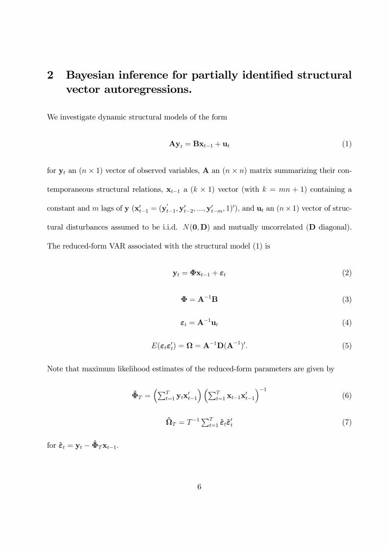
We investigate dynamic structural models of the form
Ayt = Bxt−1 + ut (1)
for yt an (n× 1) vector of observed variables, A an (n× n) matrix summarizing their con-
temporaneous structural relations, xt−1 a (k × 1) vector (with k = mn + 1) containing a
constant and m lags of y (x′t−1 = (y′
t−1,y′t−2, ...,y
′t−m, 1)
′), and ut an (n× 1) vector of struc-
tural disturbances assumed to be i.i.d. N(0,D) and mutually uncorrelated (D diagonal).
The reduced-form VAR associated with the structural model (1) is
yt = Φxt−1 + εt (2)
Φ = A−1B (3)
εt = A−1ut (4)
E(εtε′t) = Ω = A−1D(A−1)′. (5)
Note that maximum likelihood estimates of the reduced-form parameters are given by
ΦT =T
t=1 ytx′t−1
Tt=1 xt−1x
′t−1
−1(6)
ΩT = T−1T
t=1 εtε′t (7)
for εt = yt − ΦTxt−1.
6

In this section we suppose that the investigator begins with prior beliefs about the values
of the structural parameters represented by a density p(A,D,B), and show how observation
of the data YT = (x′0,y′1,y
′2, ...,y
′T )′ would lead the investigator to revise those beliefs.2
We represent prior information about the contemporaneous structural coefficients in the
form of an arbitrary prior distribution p(A). This prior could incorporate any combination
of exclusion restrictions, sign restrictions, and informative prior beliefs about elements of A.
For example, our procedure could be used to calculate the posterior distribution even if no
sign or exclusion restrictions were imposed. We also allow for interaction between the prior
beliefs about different parameters by specifying conditional prior distributions p(D|A) and
p(B|A,D) that potentially depend on A. We assume that there are no restrictions on the
lag coefficients in B other than the prior beliefs represented by the distribution p(B|A,D).
To represent prior information aboutD and B we employ natural conjugate distributions
which facilitate analytical characterization of results as well as allow for simple empirical
implementation. We use Γ(κi, τ i) priors for the reciprocals of diagonal elements of D, taken
to be independent across equations, p(D|A) =n
i=1 p(dii|A), with
p(d−1ii |A) =
τκii
Γ(κi)(d−1ii )κi−1 exp(−τ id−1ii ) for d−1ii ≥ 0
0 otherwise
, (8)
where dii denotes the (i, i) element of D. Note that κi/τ i is the prior mean for d−1ii and κi/τ
2i
its variance. Our general results allow both κi and τ i to be arbitrary functions of A.
2 Our derivations draw on insights from Sims and Zha (1998). The main difference is that they parame-terize the contemporaneous relations in terms of a single matrix, whereas we use two matrices A and D,and take advantage of the fact that the posterior distribution of D is known analytically. As a consequencethe core expression in our result (equation (21)) is simpler than their equation (10). Among other benefits,we show that the asymptotic properties of (21) can be obtained analytically.
7
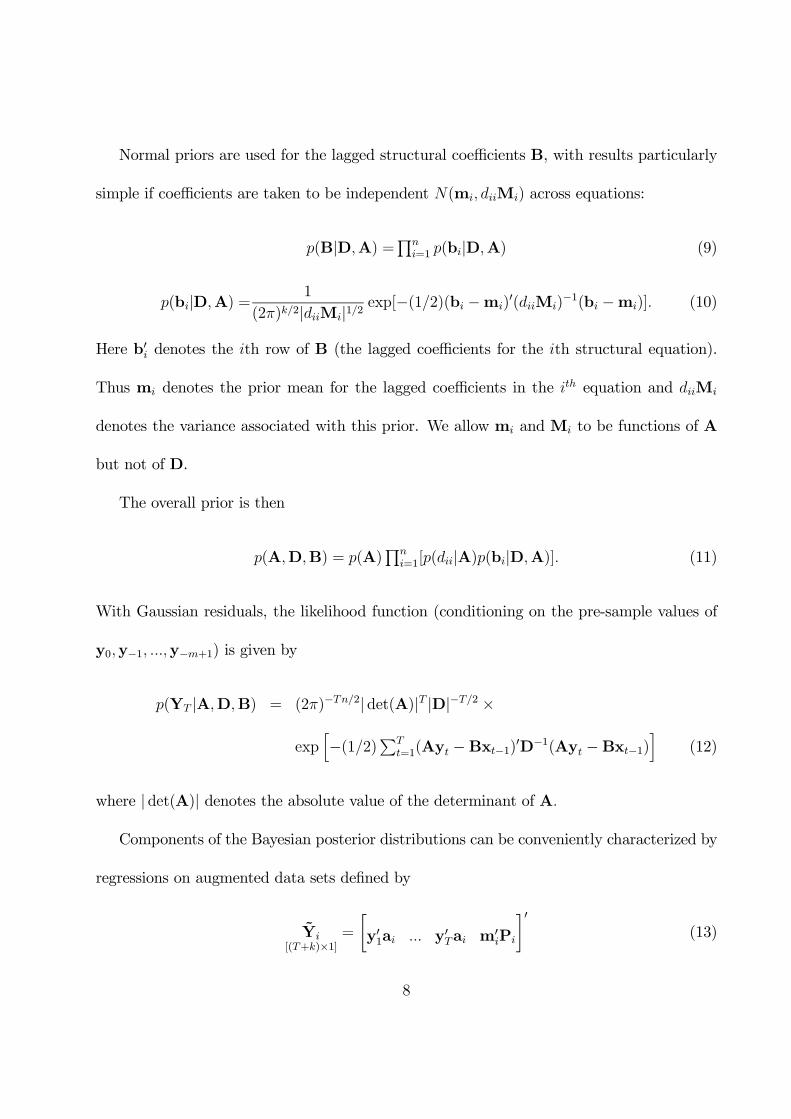
Normal priors are used for the lagged structural coefficients B, with results particularly
simple if coefficients are taken to be independent N(mi, diiMi) across equations:
p(B|D,A) =n
i=1 p(bi|D,A) (9)
p(bi|D,A) =1
(2π)k/2|diiMi|1/2exp[−(1/2)(bi −mi)
′(diiMi)−1(bi −mi)]. (10)
Here b′i denotes the ith row of B (the lagged coefficients for the ith structural equation).
Thus mi denotes the prior mean for the lagged coefficients in the ith equation and diiMi
denotes the variance associated with this prior. We allow mi and Mi to be functions of A
but not of D.
The overall prior is then
p(A,D,B) = p(A)n
i=1[p(dii|A)p(bi|D,A)]. (11)
With Gaussian residuals, the likelihood function (conditioning on the pre-sample values of
y0,y−1, ...,y−m+1) is given by
p(YT |A,D,B) = (2π)−Tn/2|det(A)|T |D|−T/2 ×
exp−(1/2)T
t=1(Ayt −Bxt−1)′D−1(Ayt −Bxt−1)
(12)
where |det(A)| denotes the absolute value of the determinant of A.
Components of the Bayesian posterior distributions can be conveniently characterized by
regressions on augmented data sets defined by
Yi[(T+k)×1]
=
y′1ai ... y′Tai m′iPi
′(13)
8
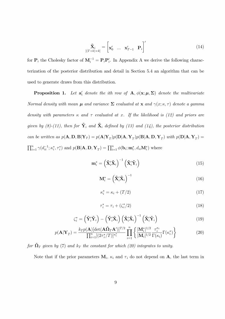
Xi[(T+k)×k]
=
x′0 ... x′T−1 Pi
′(14)
for Pi the Cholesky factor of M−1i = PiP
′i. In Appendix A we derive the following charac-
terization of the posterior distribution and detail in Section 5.4 an algorithm that can be
used to generate draws from this distribution.
Proposition 1. Let a′i denote the ith row of A, φ(x;µ,Σ) denote the multivariate
Normal density with mean µ and variance Σ evaluated at x and γ(x;κ, τ) denote a gamma
density with parameters κ and τ evaluated at x. If the likelihood is (12) and priors are
given by (8)-(11), then for Yi and Xi defined by (13) and (14), the posterior distribution
can be written as p(A,D,B|YT ) = p(A|YT )p(D|A,YT )p(B|A,D,YT ) with p(D|A,YT ) =
ni=1 γ(d
−1ii ;κ∗i , τ
∗i ) and p(B|A,D,YT ) =
ni=1 φ(bi;m
∗i , diiM
∗i ) where
m∗i =
X′
iXi
−1 X′
iYi
(15)
M∗i =
X′
iXi
−1(16)
κ∗i = κi + (T/2) (17)
τ ∗i = τ i + (ζ∗i /2) (18)
ζ∗i =Y′
iYi
−Y′
iXi
X′
iXi
−1 X′
iYi
(19)
p(A|YT ) =kTp(A)[det(AΩTA
′)]T/2
ni=1[(2τ
∗i /T )]
κ∗i
n
i=1
|M∗i |1/2
|Mi|1/2τκiiΓ(κi)
Γ(κ∗i )
(20)
for ΩT given by (7) and kT the constant for which (20) integrates to unity.
Note that if the prior parameters Mi, κi and τ i do not depend on A, the last term in
9
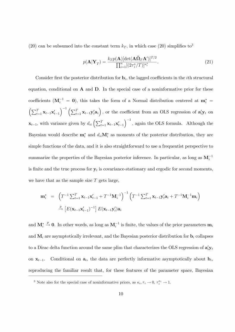
(20) can be subsumed into the constant term kT , in which case (20) simplifies to3
p(A|YT ) =kTp(A)[det(AΩTA
′)]T/2
ni=1[(2τ
∗i /T )]
κ∗i. (21)
Consider first the posterior distribution for bi, the lagged coefficients in the ith structural
equation, conditional on A and D. In the special case of a noninformative prior for these
coefficients (M−1i = 0), this takes the form of a Normal distribution centered at m∗
i =
Tt=1 xt−1x
′t−1
−1 Tt=1 xt−1y
′tai
, or the coefficient from an OLS regression of a′iyt on
xt−1, with variance given by diiT
t=1 xt−1x′t−1
−1, again the OLS formula. Although the
Bayesian would describe m∗i and diiM
∗i as moments of the posterior distribution, they are
simple functions of the data, and it is also straightforward to use a frequentist perspective to
summarize the properties of the Bayesian posterior inference. In particular, as long as M−1i
is finite and the true process for yt is covariance-stationary and ergodic for second moments,
we have that as the sample size T gets large,
m∗i =
T−1
Tt=1 xt−1x
′t−1 + T−1M−1
i
−1 T−1
Tt=1 xt−1y
′tai + T−1M−1
i mi
p→E(xt−1x
′t−1)
−1E(xt−1y′t)ai
andM∗i
p→ 0. In other words, as long asM−1i is finite, the values of the prior parametersmi
andMi are asymptotically irrelevant, and the Bayesian posterior distribution for bi collapses
to a Dirac delta function around the same plim that characterizes the OLS regression of a′iyt
on xt−1. Conditional on ai, the data are perfectly informative asymptotically about bi,
reproducing the familiar result that, for these features of the parameter space, Bayesian
3 Note also for the special case of noninformative priors, as κi, τ i → 0, τκii → 1.
10

inference is the same asymptotically as frequentist inference and correctly uncovers the true
value.
Similarly for dii, the variance of the ith structural equation, in the special case of a
noninformative prior for B (that is, when M−1i = 0) we have that ζ∗i = Ta′iΩTai. If the
priors for dii are also noninformative (κi = τ i = 0) , then the posterior expectation of d−1ii is
given by κ∗i /τ∗i = 1/(a′iΩTai), the reciprocal of the average squared residual from the OLS
regression of a′iyt on xt−1, with variance κ∗i /(τ∗i )2 = 2/[T (a′iΩTai)
2] again shrinking to zero
as T gets large. In the case of general but nondogmatic priors (κi, τ i and M−1i all finite),
as T → ∞, the value of ζ∗i /T still converges to a′iΩ0ai for Ω0 = E(εtε′t) the true variance
matrix, and the Bayesian posterior distribution for d−1ii conditional on A collapses to a point
mass at 1/(a′iΩ0ai). Hence again the priors are asymptotically irrelevant for inference about
D conditional on A.
By contrast, prior beliefs about A will not vanish asymptotically unless the elements of
A are point identified. To see this, note that in the special case of noninformative prior
beliefs about B and D, the posterior (20) simplifies to
p(A|YT ) =kTp(A)|det(AΩTA
′)|T/2
det
diag(AΩTA′)
T/2(22)
where diag(AΩTA′) denotes a matrix whose diagonal elements are the same as those ofAΩTA
′
and whose off-diagonal elements are zero. Thus when evaluated at any value of A that
diagonalizes ΩT , the posterior distribution is proportional to the prior. Recall further
from Hadamard’s Inequality that if A has full rank and ΩT is positive definite, then
detdiag(AΩTA
′)≥ det
AΩTA
′with equality only if AΩTA
′ is diagonal. Thus if we
11
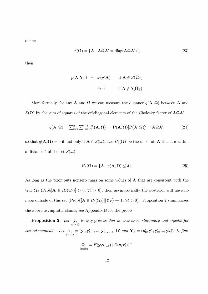
define
S(Ω) = A : AΩA′ = diag(AΩA′), (23)
then
p(A|YT ) = kTp(A) if A ∈ S(ΩT )
p→ 0 if A /∈ S(ΩT )
More formally, for any A and Ω we can measure the distance q(A,Ω) between A and
S(Ω) by the sum of squares of the off-diagonal elements of the Cholesky factor of AΩA′,
q(A,Ω) =n
i=2
i−1j=1 p
2ij(A,Ω) P(A,Ω)[P(A,Ω)]′ = AΩA′, (24)
so that q(A,Ω) = 0 if and only if A ∈ S(Ω). Let Hδ(Ω) be the set of all A that are within
a distance δ of the set S(Ω):
Hδ(Ω) = A : q(A,Ω) ≤ δ. (25)
As long as the prior puts nonzero mass on some values of A that are consistent with the
true Ω0 (Prob[A ∈ Hδ(Ω0)] > 0, ∀δ > 0), then asymptotically the posterior will have no
mass outside of this set (Prob[A ∈ Hδ(Ω0)]|YT → 1, ∀δ > 0). Proposition 2 summarizes
the above asymptotic claims; see Appendix B for the proofs.
Proposition 2. Let yt(n×1)
be any process that is covariance stationary and ergodic for
second moments. Let xt(k×1)
= (y′t,y′t−1, ...,y
′t−m+1, 1)
′ and YT = (x′0,y′1,y
′2, ...,y
′T )′. Define
Φ0(n×k)
= E(ytx′t−1) E(xtx
′t)
−1
12
Ω0(n×n)
= E(yty′t)− E(ytx
′t−1) E(xtx
′t)
−1E(xt−1y
′t)
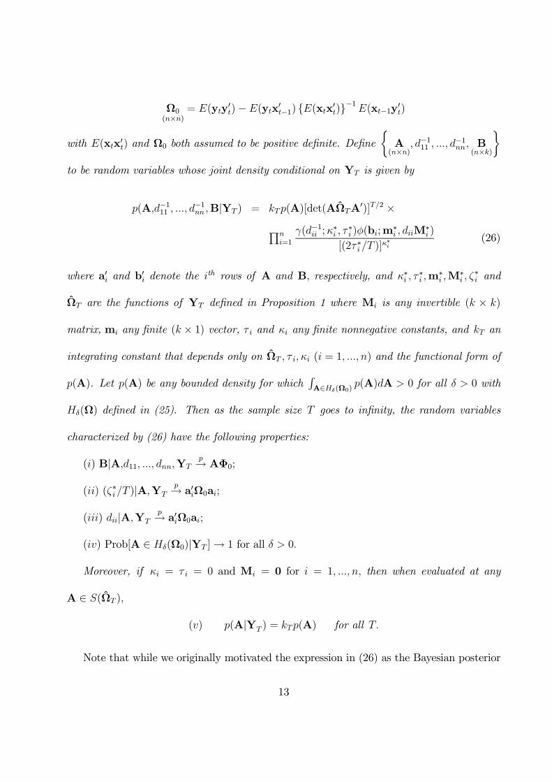
with E(xtx′t) and Ω0 both assumed to be positive definite. Define
A
(n×n), d−111 , ..., d
−1nn, B
(n×k)
to be random variables whose joint density conditional on YT is given by
p(A,d−111 , ..., d−1nn ,B|YT ) = kTp(A)[det(AΩTA
′)]T/2 ×
ni=1
γ(d−1ii ;κ∗i , τ∗i )φ(bi;m
∗i , diiM
∗i )
[(2τ ∗i /T )]κ∗i
(26)
where a′i and b′i denote the ith rows of A and B, respectively, and κ∗i , τ∗i ,m
∗i ,M
∗i , ζ
∗i and
ΩT are the functions of YT defined in Proposition 1 where Mi is any invertible (k × k)
matrix, mi any finite (k × 1) vector, τ i and κi any finite nonnegative constants, and kT an
integrating constant that depends only on ΩT , τ i, κi (i = 1, ..., n) and the functional form of
p(A). Let p(A) be any bounded density for whichA∈Hδ(Ω0)
p(A)dA > 0 for all δ > 0 with
Hδ(Ω) defined in (25). Then as the sample size T goes to infinity, the random variables
characterized by (26) have the following properties:
(i) B|A,d11, ..., dnn,YTp→ AΦ0;
(ii) (ζ∗i /T )|A,YT
p→ a′iΩ0ai;
(iii) dii|A,YT
p→ a′iΩ0ai;
(iv) Prob[A ∈ Hδ(Ω0)|YT ]→ 1 for all δ > 0.
Moreover, if κi = τ i = 0 and Mi = 0 for i = 1, ..., n, then when evaluated at any
A ∈ S(ΩT ),
(v) p(A|YT ) = kTp(A) for all T.
Note that while we originally motivated the expression in (26) as the Bayesian posterior
13

distribution for a Gaussian structural VAR, the results in Proposition 2 do not assume that
the actual data are Gaussian or even that they follow a VAR. Nor does the proposition
make any use of the fact that there exists a Bayesian interpretation of these formulas. The
proposition establishes that as long as the prior assigns nonzero probability to a subset of A
that diagonalizes the value Ω0 defined in the proposition, then asymptotically the posterior
density will be confined to that subset and at any point within the set will converge to some
constant times the value of the prior density at that point.
In the special case where the model is point-identified, there exists only one allowable
value of A for which AΩ0A′ is diagonal. Provided that p(A) is nonzero in all neighborhoods
including that point, the posterior distribution collapses to the Dirac delta function at this
value of A. This reproduces the familiar result that under point identification, the priors
on all parameters (A,D, and B) are asymptotically irrelevant and Bayesian inference is
asymptotically equivalent to maximum likelihood estimation, producing consistent estimates
of parameters.
3 Priors implicit in the traditional approach to sign-
identified VARs.
In this section we characterize the prior distributions that are implicit in the approach to
sign-restricted VARs developed by Rubio-Ramírez et al. (2010). Their focus was on the
mapping between the VAR residuals εt and a vector of unit-variance structural shocks vt:
εt = Hvt vt ∼ N(0, In). (27)
14

Their algorithm begins by generating an (n × n) matrix X = [xij ] of independent N(0, 1)
variates and then calculating the decomposition X = QR where Q is an orthogonal matrix
and R is upper triangular. From this a candidate draw for the contemporaneous response
to the vector of structural shocks is calculated as
H = PQ (28)
for P the Cholesky factor of the variance matrix of the reduced-form innovations:
Ω = PP′. (29)
This algorithm can be viewed as generating draws from a Bayesian prior distribution for
H conditional on Ω, the properties of which we now document. Note that the first column
of Q is simply the first column of X normalized to have unit length:
q11
...
qn1
=
x11/x211 + · · ·+ x2n1
...
xn1/x211 + · · ·+ x2n1
. (30)
In the special case when n = 2, q11 has the interpretation as the cosine of θ, the angle defined
by the point (x11, x21). In this case, the fact that Q is an orthogonal matrix will result in
half the draws being the rotation matrix associated with θ and the other half the reflection
matrix:
Q =
cos θ − sin θ
sin θ cos θ
with probability 1/2
cos θ sin θ
sin θ − cos θ
with probability 1/2
. (31)
15

Independence of x11 and x21 ensures that θ will have a uniform distribution over [−π, π]. It
is in this sense that the prior implicit in the procedure (28) is thought to be uninformative.
However, a prior that is uninformative about some features of the parameter space can
turn out to be informative about others. It is not hard to show that each element of (30)
has a marginal density given by4
p(qi1) =
Γ(n/2)Γ(1/2)Γ((n−1)/2)(1− q2i1)
(n−3)/2 if qi1 ∈ [−1, 1]
0 otherwise
. (32)
Note next that the (1, 1) element of (28) therefore implies a prior distribution for the effect
of a one-standard-deviation increase in structural shock number 1 on variable number 1 that
is characterized by the random variable h11 = p11q11 =√ω11q11 for ω11 the (1, 1) element of
Ω. In other words, the implicit prior belief about the effect of this structural shock has the
distribution of√ω11 times the random variable in (32). Note that if we invoke no further
normalization or sign restrictions, “shock number 1” would be associated with no different
identifying information than “shock number j”. Invariance of the algorithm5 and the
4 Note from Theorem 3.1 of Devroye (1986, p.403) that the variable yi1 = q2i1,
yi1 =x2i1
x211 + · · ·+ x2n1,
has a Beta(1/2,(n− 1)/2) distribution:
p(yi1) =
Γ(n/2)
Γ(1/2)Γ((n−1)/2)y(1/2)−1i1 (1− yi1)((n−1)/2)−1 if yi1 ∈ [0, 1]
0 otherwise.
The density of qi1 =√yi1 in (32) is then obtained using the change-of-variables formula. Alternatively, one
can verify directly that when θ ∼ U(−π, π), the random variables ± cos θ and ± sin θ each have a densitythat is given by the special case of (32) corresponding to n = 2.
5 This conclusion can also be verified by direct manipulation of the relevant equations, as shown inAppendix C.
16

change-of-variables formula for probabilities thus implies a prior density for hij = ∂yit/∂ujt,
the effect on impact of structural shock j on observed variable i given by
p(hij|Ω) =
Γ(n/2)Γ(1/2)Γ((n−1)/2)
1√ωii
(1− h2ij/ωii)(n−3)/2 if hij ∈ [−√ωii,
√ωii]
0 otherwise
. (33)
Panel A of Figure 1 plots this density for two different values of n. When there are n = 2
variables in the VAR, this prior regards impacts of ±√ωii as more likely than 0. By contrast,
when there are n ≥ 4 variables in the VAR, impacts near 0 are regarded as more likely. The
distribution is only uniform in the case n = 3.
Alternatively, researchers are more often interested in the effect of a structural shock
normalized by some definition, for example, the effect on observed variable 2 of a shock that
increases observed variable number 1 by one unit. Such an object is characterized by the
ratio of the (2,1) to the (1,1) element of (28):6
h∗21 =∂y2t∂u∗1t
=p21q11 + p22q21
p11q11=
p21p11
+p22p11
x21x11
= ω21/ω11 +
ω22 − ω221/ω11
ω11
x21x11
.
Recall that the ratio of independent N(0, 1) has a standard Cauchy distribution. Invariance
properties again establish that the choice of subscripts 1 and 2 is irrelevant. Thus for any
i = j,
h∗ij|Ω ∼ Cauchy(c∗ij, σ∗ij) (34)
6 The final equation here is derived from the upper (2× 2) block of (29):
ω11 ω21ω21 ω22
=
p211 p11p21p11p21 p221 + p
222
.
17
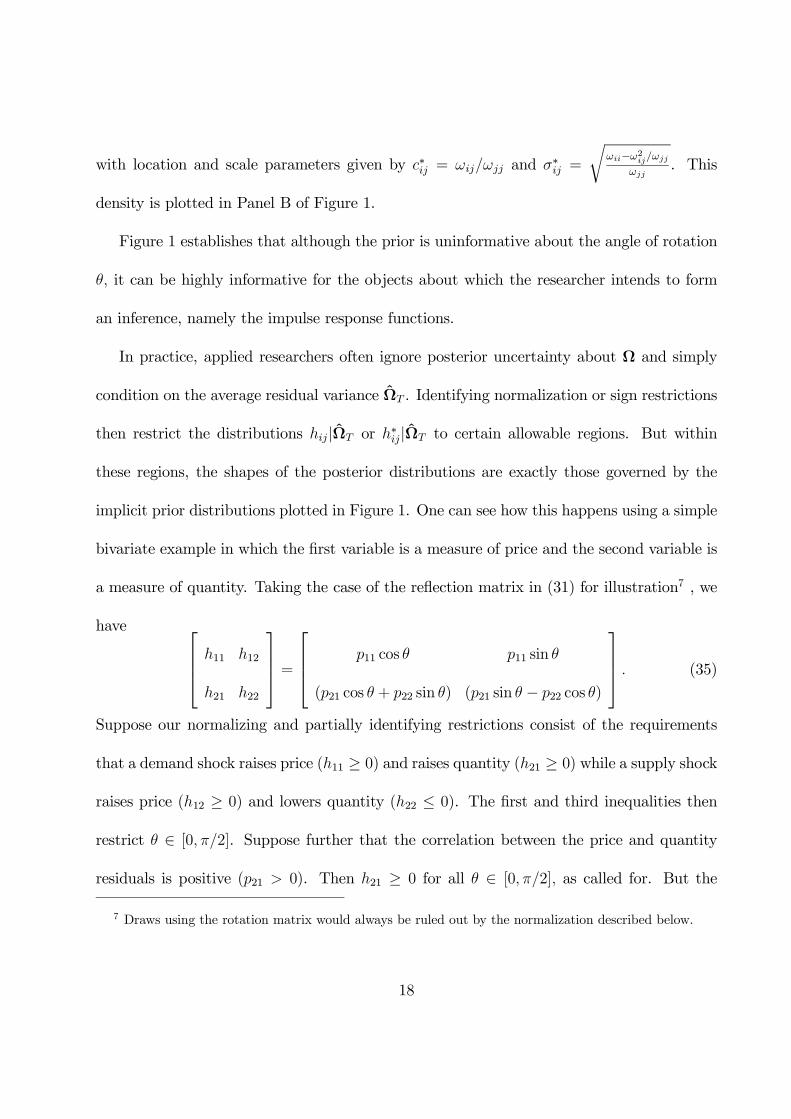
with location and scale parameters given by c∗ij = ωij/ωjj and σ∗ij =
ωii−ω2ij/ωjj
ωjj. This
density is plotted in Panel B of Figure 1.
Figure 1 establishes that although the prior is uninformative about the angle of rotation
θ, it can be highly informative for the objects about which the researcher intends to form
an inference, namely the impulse response functions.
In practice, applied researchers often ignore posterior uncertainty about Ω and simply
condition on the average residual variance ΩT . Identifying normalization or sign restrictions
then restrict the distributions hij|ΩT or h∗ij|ΩT to certain allowable regions. But within
these regions, the shapes of the posterior distributions are exactly those governed by the
implicit prior distributions plotted in Figure 1. One can see how this happens using a simple
bivariate example in which the first variable is a measure of price and the second variable is
a measure of quantity. Taking the case of the reflection matrix in (31) for illustration7 , we
have
h11 h12
h21 h22
=
p11 cos θ p11 sin θ
(p21 cos θ + p22 sin θ) (p21 sin θ − p22 cos θ)
. (35)
Suppose our normalizing and partially identifying restrictions consist of the requirements
that a demand shock raises price (h11 ≥ 0) and raises quantity (h21 ≥ 0) while a supply shock
raises price (h12 ≥ 0) and lowers quantity (h22 ≤ 0). The first and third inequalities then
restrict θ ∈ [0, π/2]. Suppose further that the correlation between the price and quantity
residuals is positive (p21 > 0). Then h21 ≥ 0 for all θ ∈ [0, π/2], as called for. But the
7 Draws using the rotation matrix would always be ruled out by the normalization described below.
18

condition h22 ≤ 0 requires θ ∈ [0, θ] where θ is the angle in [0, π/2] for which cot θ = p21/p22.
Recall that the response of quantity to a supply shock that raises the price by 1% is given by
the ratio of the (2,2) to the (2,1) element in (35): h∗22 = (p21/p11)− (p22/p11) cot θ. As θ goes
from 0 to θ, h∗22 varies from −∞ to 0. One can verify directly8 that when θ ∼ U(−π, π),
cot θ ∼ Cauchy(0,1). Thus when the correlation between the OLS residuals is positive, the
posterior distribution of h∗22 is a Cauchy(c∗22, σ
∗22) truncated to be negative.
The value of h∗21 (which measures the response of quantity to a demand shock that raises
the price by 1%) is given by h∗21 = (p21/p11) + (p22/p11) tan θ. As θ varies from 0 to θ, this
ranges from
hL =p21p11
+p22p11
× 0 =ω21ω11
. (36)
to
hH =p21p11
+p22p11
p22p21
=p221 + p222p11p21
=ω22ω21
(37)
Note that the magnitude h∗21 usually goes by another name— it is the short-run price
elasticity of supply, while h∗22 is just the short-run price elasticity of demand. We have
thus seen that, when the correlation between price and quantity is positive, the posterior
distribution for the demand elasticity will be the original Cauchy(c∗22, σ∗22) truncated to
be negative, while the posterior distribution for the supply elasticity will be the original
Cauchy(c∗21, σ∗21) truncated to the interval [hL, hH ].
Alternatively, if price and quantity are negatively correlated, the magnitudes in (36)
and (37) would be negative numbers. In this case, the posterior distribution for the supply
8 See for example Gubner (2006, p.194). This of course is just a special case of the general result in (34).
19
elasticity will be the original Cauchy(c∗21, σ∗21) truncated to be positive, while that for the
demand elasticity will be the original Cauchy(c∗22, σ∗22) truncated to the interval [hH , hL].
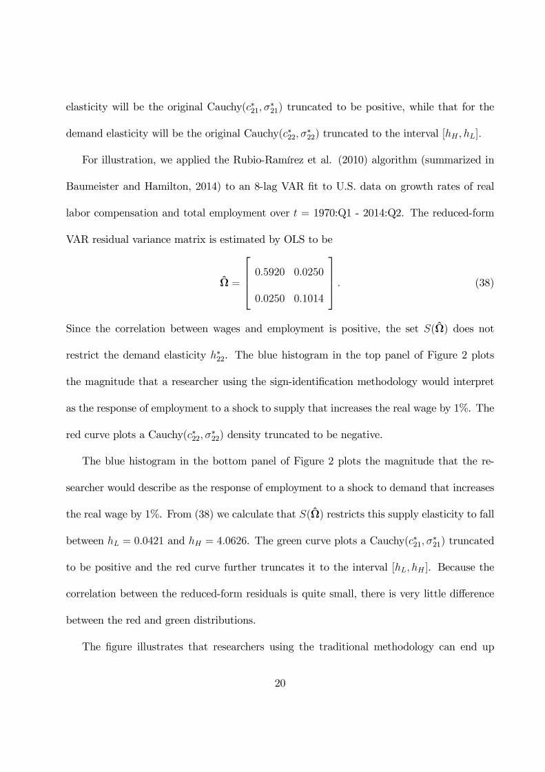
For illustration, we applied the Rubio-Ramírez et al. (2010) algorithm (summarized in
Baumeister and Hamilton, 2014) to an 8-lag VAR fit to U.S. data on growth rates of real
labor compensation and total employment over t = 1970:Q1 - 2014:Q2. The reduced-form
VAR residual variance matrix is estimated by OLS to be
Ω =
0.5920 0.0250
0.0250 0.1014
. (38)
Since the correlation between wages and employment is positive, the set S(Ω) does not
restrict the demand elasticity h∗22. The blue histogram in the top panel of Figure 2 plots
the magnitude that a researcher using the sign-identification methodology would interpret
as the response of employment to a shock to supply that increases the real wage by 1%. The
red curve plots a Cauchy(c∗22, σ∗22) density truncated to be negative.
The blue histogram in the bottom panel of Figure 2 plots the magnitude that the re-
searcher would describe as the response of employment to a shock to demand that increases
the real wage by 1%. From (38) we calculate that S(Ω) restricts this supply elasticity to fall
between hL = 0.0421 and hH = 4.0626. The green curve plots a Cauchy(c∗21, σ∗21) truncated
to be positive and the red curve further truncates it to the interval [hL, hH ]. Because the
correlation between the reduced-form residuals is quite small, there is very little difference
between the red and green distributions.
The figure illustrates that researchers using the traditional methodology can end up
20
performing hundreds of thousands of calculations, ostensibly analyzing the data, but in the
end are doing nothing more than generating draws from a prior distribution that they never
even acknowledged that they had assumed!
While one might suppose that the distributions in Figures 1 and 2 are simply an un-
intended side effect of the Haar prior, the problem is much more pervasive. In fact, any
uniform prior distribution for the effect of a structural shock on one variable necessarily im-
plies a nonuniform prior distribution for the effects on other variables or of other structural
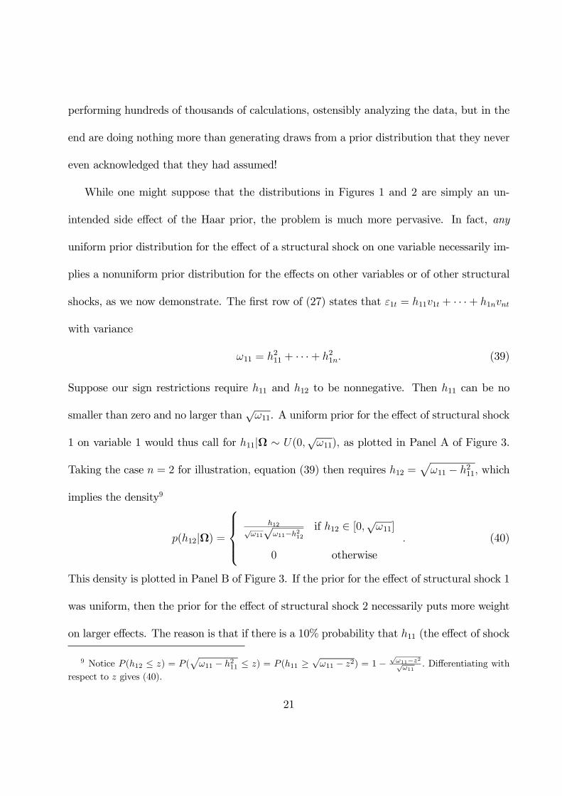
shocks, as we now demonstrate. The first row of (27) states that ε1t = h11v1t + · · ·+ h1nvnt
with variance
ω11 = h211 + · · ·+ h21n. (39)
Suppose our sign restrictions require h11 and h12 to be nonnegative. Then h11 can be no
smaller than zero and no larger than√ω11. A uniform prior for the effect of structural shock
1 on variable 1 would thus call for h11|Ω ∼ U(0,√ω11), as plotted in Panel A of Figure 3.
Taking the case n = 2 for illustration, equation (39) then requires h12 =ω11 − h211, which
implies the density9
p(h12|Ω) =
h12√ω11√
ω11−h212
if h12 ∈ [0,√ω11]
0 otherwise
. (40)
This density is plotted in Panel B of Figure 3. If the prior for the effect of structural shock 1
was uniform, then the prior for the effect of structural shock 2 necessarily puts more weight
on larger effects. The reason is that if there is a 10% probability that h11 (the effect of shock
9 Notice P (h12 ≤ z) = P (ω11 − h211 ≤ z) = P (h11 ≥
√ω11 − z2) = 1 −
√ω11−z2√ω11
. Differentiating with
respect to z gives (40).
21
1) is less than 0.1√ω11 (as a uniform prior on h11 would require), then there must be a 10%
probability that h12 (the effect of shock 2) exceedsω11 − (0.1)2ω11 =
√0.99
√ω11. Thus
the density of h12 in Panel B would be required to go off to infinity as h12 approaches√ω11
if we wanted to use a uniform prior for h11. One can also show that a uniform prior for the
effect of structural shock 1 on variable 1, h11|Ω ∼ U(0,√ω11), implies a nonuniform prior
for the effect of structural shock 1 on variable 2—we can’t even pick a single shock by itself
about which we could claim that our prior is truly uninformative!10
Could we avoid such problems by posing the prior directly in terms of an unconditional
density p(H) instead of the conditional density p(H|Ω)? Suppose we insisted on relatively
flat priors for h11 and h21, which say correspond to the effect of a one-standard-deviation
shock to monetary policy on interest rates and output. The natural use that researchers
and policymakers would make of the results would be calculating the effect on output if the
Fed raised interest rates by 25 basis points, namely h21/h11. A uniform prior on h11 and h21
implies a nonuniform prior for h21/h11.
These are all illustrations of the general principle that a uniform prior for any parameter
implies a nonuniform prior for nonlinear functions of that parameter (e.g., Datta and Ghosh,
1996). Because the objects of interest in structural VARs are highly nonlinear functions of
the underlying parameters, the quest for “noninformative” priors for structural VARs is
destined to fail.
Our recommendation is that rather than regard these procedures as something that can
10 The distribution for h21|Ω is characterized by the equation ω21 = h11h21 + h12ω22 − h221 where the
distributions of h11|Ω and h12|Ω are as displayed in Figure 3.
22

be implemented without thinking, it is preferable to spell out explicitly the class of structural
models that the researcher has in mind and exactly what is known and unknown about the
model. Our proposed formulation of the problem does exactly this. The coefficients in A are
written in the natural units of a true structural model in which the elements correspond to
parameters governing elasticities, policy rules, and first-order conditions. When the model is
written in this way, it is possible (as we illustrate in Section 5) to draw on literally hundreds
of previous studies for what might be known about plausible values for the parameters, as
well as to find the correct implications for any objects of interest when little is known about
the structural model. By contrast, prior beliefs about the elements of H would at best
be based on loose intuition about how the structural parameters in A interact when the
matrix is inverted. We nevertheless note that, since Proposition 1 describes the inference
for an arbitrary set of prior beliefs about A, it immediately also characterizes inference if
for some reason the researcher preferred to represent these in the form of prior beliefs about
the elements of A−1.
4 Sign restrictions for higher-horizon impacts.
In an effort to try to gain additional identification, many applied researchers impose sign re-
strictions not just on the time-zero structural impacts ∂yt/∂u′t but also on impacts ∂yt+s/∂u
′t
for some horizons s = 0, 1, ..., S. These are given by
∂yt+s
∂u′t= ΨsA
−1 (41)
23

for Ψs the first n rows and columns of Fs for
F =
Φ1 Φ2 · · · Φm−1 Φm
In 0 · · · 0 0
...... · · · ...
...
0 0 · · · In 0
(42)
yt = c+Φ1yt−1 +Φ2yt−2 + · · ·+Φmyt−m + εt.
Beliefs about higher-order impacts are of necessity joint beliefs aboutA andB. For example,
∂yt
∂u′t= A−1 (43)
∂yt+1
∂u′t= Φ1A
−1. (44)
If Φ1 is diagonal with negative elements, the signs of ∂yt+1/∂u′t are opposite those of A
−1
itself. In this case, as the sample size grows to infinity, there will be no posterior distribution
satisfying a restriction such as ∂yit/∂ujt and ∂yi,t+1/∂ujt are both positive. In a finite sam-
ple, a simulated draw from the posterior distribution purporting to impose such a restriction
would at best be purely an artifact of sampling error. Canova and Paustian (2011) demon-
strated using a popular macro model that implications for the signs of structural multipliers
beyond the zero horizon (∂yt+s/∂u′t for s > 0) are generally not robust.
In our parameterization prior beliefs about structural impacts for s > 0 would be repre-
sented in the form of the prior distribution p(B|A,D). Our recommendation is that nondog-
matic priors should be used for this purpose, since we have seen the data are asymptotically
fully informative about the posterior p(B|A,D,YT ).
24
A common source of the expectation that signs of ∂yt+s/∂u′t should be the same as
those of ∂yt/∂u′t is a prior expectation that Φ1 is not far from the identity matrix and
that elements of Φ2, ...,Φm are likely small. Nudging the unrestricted OLS estimates in the
direction of such a prior has long been known to help improve the forecasting accuracy of a
VAR.11 This suggests that we might want to use priors for A and B that imply a value for
η = E(Φ) given by
η(n×k)
=
In(n×n)
0[n×(k−n)]
. (45)
As noted by Sims and Zha (1998), since B = AΦ, this calls for setting the prior mean for
B|A to be E(B|A) = Aη, suggesting a prior mean for bi given by mi = E(bi|A) = η′ai.
We can also follow Doan, Litterman and Sims (1984) as modified by Sims and Zha (1998) in
putting more confidence in our prior beliefs that higher-order lags are zero, as we describe
in detail in Section 5.4.
Some researchers may want to use additional prior information about structural dynam-
ics. In the example in the following section, we consider a prior belief that a labor demand
shock should have little permanent effect on the level of employment. We have found it
convenient to implement these as supplements to our general recommendations, where we
could put as little weight as we wanted on the general recommendations by specifying λ0 in
expression (58) to be sufficiently large. For example, had the additional information that hi
linear combinations (represented by Ribi) should be close to some expected value ri, where
ri could be a function of A. As in Theil (1971, pp.347-49) we can represent this additional
11 See for example Doan, Litterman and Sims (1984), Litterman (1986), and Smets and Wouters (2003).
25

information in the form of hi pseudo observations
ri(hi×1)
= Ri(hi×k)
bi(k×1)
+ vi(hi×1)
vi ∼ N(0, dii Vi(hi×hi)
) (46)
allowing us to simply replace (13) and (14) with12
Yi[(T+k+hi)×1]
=
a′iy1 · · · a′iyT m′iPi r′iPVi
′(47)
Xi[(T+k+hi)×k]
=
x0 · · · xT−1 Pi R′iPVi
′(48)
for M−1i = PiP
′i and V
−1i = PViP
′Vi.
Although such priors can help improve inference about the structural parameters in a
given observed sample, they do not change any of the asymptotics in Proposition 2.
5 Application: Bayesian inference in a model of labor
supply and demand.
In this section we illustrate these methods using the example of labor supply and labor
demand introduced in Section 3. The goal here is to elevate such prior information from
something that the researcher imposes mechanically without consideration to something
that is explicitly acknowledged and can be motivated from economic theory and empirical
evidence from other data sets. Consider structural dynamic labor demand and supply curves
12 This is numerically identical to using bi|A,D ∼ N(mi, diiMi) as a unified prior in (10) with M−1i =
M−1i +R′
iV−1i Ri and mi = Mi(M
−1i mi +R
′iV
−1i ri).
26
of the form:
demand: ∆nt = kd + βd∆wt + bd11∆wt−1 + bd12∆nt−1 + bd21∆wt−2 + bd22∆nt−2 +
· · ·+ bdm1∆wt−m + bdm2∆nt−m + udt
supply: ∆nt = ks + αs∆wt + bs11∆wt−1 + bs12∆nt−1 + bs21∆wt−2 + bs22∆nt−2 +
· · ·+ bsm1∆wt−m + bsm2∆nt−m + ust . (49)
Here ∆nt is the growth rate of total U.S. employment,13 ∆wt is the growth rate of real
compensation per hour,14 βd is the short-run wage elasticity of demand, and αs is the
short-run wage elasticity of supply. Note that the system (49) is a special case of (1) with
yt = (∆wt,∆nt)′ and
A =
−βd 1
−αs 1
. (50)
OLS estimation of the reduced-form (2) for this system with m = 8 lags and t = 1970:Q1
through 2014:Q2 led to the estimate of the reduced-form residual variance matrix Ω =
T−1T
t=1 εtε′t reported in (38).
5.1 Maximum likelihood estimates.
As in Shapiro and Watson (1988), for any given α we can find the maximum likelihood
estimate of β by an IV regression of ε2t on ε1t using ε2t − αε1t as instruments, where εit are
13 The level nt was measured as 100 times the natural log of the seasonally adjusted number of people onnonfarm payrolls during the third month of quarter t from series PAYEMS downloaded August 2014 fromhttp://research.stlouisfed.org/fred2/.
14 The level wt was measured as 100 times the natural log of seasonally adjusted real compensa-tion per hour for the nonfarm business sector from series COMPRNFB downloaded August 2014 fromhttp://research.stlouisfed.org/fred2/.
27

the residuals from OLS estimation of the reduced-form VAR,
β(α) =
Tt=1(ε2t − αε1t)ε2tTt=1(ε2t − αε1t)ε1t
=(ω22 − αω12)
(ω12 − αω11), (51)
for ωij the (i, j) element of Ω. One can verify directly that any pair (α, β) satisfying (51)
produces a diagonal matrix for AΩA′.
The top panel of Figure 4 plots the function β(α) for these data. Any pair (α, β) lying
on these curves would maximize the likelihood function, and there is no basis in the data
for preferring one point on the curves to any other.
If we restrict the supply elasticity α to be positive and the demand elasticity β to be
negative, we are left with the lower right quadrant in the figure. When, as in this data
set, the OLS residuals are positively correlated, the sign restrictions are consistent with any
β ∈ (−∞, 0), but require α to fall in the interval (hL, hH) defined in (36)-(37). We earlier
derived these bounds considering allowable angles of rotation but it is also instructive to
explain their intuition in terms of a structural interpretation of the likelihood function.15
Note that hL is the estimated coefficient from an OLS regression of ε2t on ε1t, which is a
weighted average of the positive supply elasticity α and negative demand elasticity β (see
for example Hamilton, 1994, equation [9.1.6]). Hence the MLE for β can be no larger than
hL and the MLE for α can be no smaller than hL. The fact that the MLE for β can be no
larger than hL is not a restriction, because we have separately required that β < 0 and in
the case under discussion, hL > 0. However, the inference that α can be no smaller than hL
puts a lower bound on α. At the other end, the OLS coefficient from a regression of ε1t on
15 Leamer (1981) discovered these points in a simple OLS setting years ago.
28

ε2t (that is, h−1H ) turns out to be a weighted average of α−1 and β−1, requiring β−1 < h−1H
(again not binding when hH > 0) and α−1 > h−1H ; the latter gives us the upper bound that
α < hH . This is the intuition for why hL < α < hH .
The bottom panel in Figure 4 plots contours of the concentrated likelihood function, that
is, contours of the function: T log | det(A)| − (T/2) logdet
diag(AΩA
′)
.The data are
quite informative that α and β should be close to the values that diagonalize Ω, that is, that
α and β are close to the function β = β(α) shown in black.
The set S(Ω) in expression (23) is calculated for this example as follows. When the
correlation between the VAR residuals ω12 is positive, S(Ω) is the set of all A in (50) such
that β ≤ 0, (ω21/ω11) ≤ α ≤ (ω22/ω21), and β = (ω22− αω12)/(ω12 −αω11), in other words,
the set of points on the black curve in Figure 4 between hL and hH .
5.2 Prior information about elasticities.
While the frequentist would regard any of the points in S(Ω) as equally plausible, from the
standpoint of economic theory that is surely not the case; for example, a demand elasticity of
−100 would not be consistent with any coherent economic model. We propose to represent
prior information about α and β using Student t distributions with ν degrees of freedom.
Note that this includes the Cauchy distribution in (34) as a special case when ν = 1. One
benefit of using ν ≥ 3 is that the posterior distributions for α and β would then be guaranteed
to have finite mean and variance. Our proposal is that the location and scale parameters for
these distributions should be chosen on the basis of prior information about these elasticities.
Hamermesh’s (1996) survey of microeconometric studies concluded that the absolute
29

value of the elasticity of labor demand is between 0.15 and 0.75. Lichter, Peichl, and
Siegloch’s (2014) meta-analysis of 942 estimates from 105 different studies favored values
at the lower end of this range. On the other hand, theoretical macro models can imply a
value of 2.5 or higher (Akerlof and Dickens, 2007; Galí, Smets, and Wouters, 2012). A prior
for β that reflects the uncertainty associated with these findings could be represented with
a Student t distribution with location parameter cβ = −0.6, scale parameter σβ = 0.6, and
degrees of freedom νβ = 3, truncated to be negative. This places a 5% probability on values
of β < −2.2 and another 5% probability on values above −0.1.
In terms of the labor supply elasticity, a key question is whether the increase in wages is
viewed as temporary or permanent. A typical assumption is that the income and substitu-
tion effects cancel, in which case there would be zero observed response of labor supply to a
permanent increase in the real wage (Kydland and Prescott, 1982). On the other hand, the
response to a temporary wage increase is often interpreted as the Frisch (or compensated
marginal utility) elasticity, about which there are again quite different consensuses in the
micro and macro literatures. Chetty et al. (2013) reviewed 15 different quasi-experimental
studies all of which implied Frisch elasticities below 0.5. A separate survey of microeconomet-
ric studies by Reichling and Whalen (2012) concluded that the Frisch elasticity is between
0.27 and 0.53. By contrast, values above one or two are common in the macroeconomic liter-
ature (see e.g., Kydland and Prescott, 1982, Cho and Cooley, 1994, and Smets and Wouters,
2007). For the prior used for the short-run elasticity α in this study, we specified cα = 0.6,
σα = 0.6, and να = 3, which associates a 90% probability to α ∈ (0.1, 2.2).
30

The prior distribution p(A) is thus taken to be the product of these two truncated
Student t densities, which is written out explicitly in equation (56) below. Contours for
this prior distribution are provided in the top panel of Figure 5, while the bottom panel
displays contours for the posterior distribution that would result if we used only this prior
p(A) with no additional information about D or B. The observed data contain sufficient
information to cause all of the posterior distribution to fall within a close neighborhood of
S(Ω). But whereas the frequentist regards all points within this set as equally plausible,
a sensible person with knowledge of the literature would regard values such as α = 0.5,
β = −0.3 as much more plausible than α = 0.06, β = −9.5. The Bayesian approach gives
the analyst a single coherent framework for combining uncertainty caused by observing a
limited data set (that is, uncertainty about the true value of Ω) with uncertainty about the
correct structure of the model itself (that is, uncertainty about points within S(Ω)), which
combined uncertainty is represented by the contours in the bottom panel of Figure 5.
5.3 Long-run restrictions.
We also illustrate how inference could be improved by making use of additional sources of
outside information about the long-run labor supply elasticity. Let yt = (wt, nt)′ denote the
levels of the variables so that yt = ∆yt. From (41) the effect of the structural shocks on the
future levels of wages and employment is given by
∂yt+s
∂u′t=
∂∆yt+s
∂u′t+∂∆yt+s−1
∂u′t+ · · ·+ ∂∆yt
∂u′t
= ΨsA−1 +Ψs−1A
−1 + · · ·+Ψ0A−1 (52)
31

with a permanent or long-run effect given by
lims→∞
∂yt+s
∂u′t= (Ψ0 +Ψ1 +Ψ2 + · · · )A−1 = (In −Φ1 −Φ2 − · · · −Φm)
−1A−1.
The long-run effect of a labor demand shock on employment is given by the (2, 1) element
of this matrix. Recalling that Φj = A−1Bj this long-run elasticity would be zero if and only
if the above matrix is upper triangular, or equivalently if and only if the following matrix is
upper triangular
A(In −Φ1 −Φ2 − · · · −Φm) = A−B1 −B2 − · · · −Bm (53)
requiring 0 = −αs − bs11 − bs21 − · · · − bsm1 or
bs11 + bs21 + · · ·+ bsm1 = −αs. (54)
If we were to insist that (54) has to hold exactly, then the model would become just-
identified even in the absence of any information about αs or βd, and indeed hundreds of
empirical papers have used exactly such a procedure to perform structural inference using
VARs.16 We propose instead to represent the idea as a prior belief of the form
(bs11 + bs21 + · · ·+ bsm1)|A,D ∼ N(−αs, d22V2). (55)
Note that our proposal is a strict generalization of the existing approach, in that (55) becomes
(54) in the special case when V2 → 0. We would further argue that our method is a
strict improvement over the existing approach in several respects. First, (54) is usually
16 See for example Shapiro and Watson (1988), Blanchard and Quah (1989), and Galí (1999).
32

implemented by conditioning on the reduced-form estimates Φ. By contrast, our approach
will generate the statistically optimal joint inference about A and B taking into account
the fact that both are being estimated with error. Second, we would argue that the claim
that (54) is known with certainty is indefensible. A much better approach in our view is to
acknowledge openly that (54) is a prior belief about which any reasonable person would have
some uncertainty. Granted, an implication of Proposition 2 is that some of this uncertainty
will necessarily remain even if we had available an infinite sample of observations on y.
However, our position is that this uncertainty about the specification should be openly
acknowledged and reported as part of the results, and indeed as we have demonstrated this
is exactly what is accomplished using the algorithm suggested in Proposition 1.
Note that our recommended approach also helps address some of the concerns about long-
run restrictions raised by Faust and Leeper (1997). For example, rather than dogmatically
impose that coefficients beyond some fixed lag are all zero, our approach instead allows the
researcher to shrink coefficients toward zero gradually as the lag length increases up to some
largem, with the pace of the shrinkage governed by choice of the parameter λ1 used to define
v1 in expression (58).
5.4 Implementation of the estimation algorithm.
Before discussing the results, we document step by step how our algorithm is implemented
for this example.17 Readers not interested in these technical details can skip this section.
17 Code to replicate these results and to apply in more general settings is available athttp://econweb.ucsd.edu/~jhamilton/BHcode.zip.
33
5.4.1 Setting the parameters for the prior distributions
Step 1a: Prior for the elasticities p(A). Collect the unknown elements of A in the
vector α = (α, β)′ with prior p(A) the product of truncated Student t densities:
p(α) =
f(α;cα,σ,ν)1−F (0;cα,σ,ν)
f(β;cα,σ,ν)F (β;cα,σ,ν)
if α ≥ 0 and β ≤ 0
0 otherwise
(56)
where f(x; c, σ, ν) denotes the density for a Student t variable with location c, scale σ, and
degrees of freedom ν evaluated at x,
f(x; c, σ, ν) =Γ(ν+1
2)√
νπσΓ(ν/2)
!1 +
(x− c)2
σ2ν
"−(ν+1)/2(57)
and F (.) the cumulative distribution function F (x; c, σ, ν) = x
−∞f(z; c, σ, ν)dz. We set
cα = 0.6, cβ = −0.6, σ = 0.6, and ν = 3.
Step 1b: Prior for the inverse of the structural variances p(dii|A). Prior beliefs
about structural variances should reflect in part the scale of the underlying data. Let
eit denote the residuals from an 8th-order univariate autoregression fit to series i and S =
T−1T
t=1 e1te2t the sample variance matrix of these univariate residuals. We set κi = 2,
which given equation (17) puts a weight on our prior equivalent to 2κi = 4 observations of
data. The prior mean for d−1ii = κi/τ i is chosen to equal the reciprocal of the ith diagonal
element of ASA′, that is, τ i(α) = κia
′iSai.
Step 1c: Prior for the lagged structural coefficients p(bi|A,D). Compute the
prior mean mi(α) = η′ai with η defined in (45). Doan et al. (1984) suggested that we
should have greater confidence in our expectation that coefficients on higher lags are zero,
34

represented by smaller diagonal elements forMi associated with higher lags. Let√sii denote
the estimated standard deviation of a univariate 8th-order autoregression fit to variable i and
define v′1(1×m)
=#1/(12λ1
$, 1/(22λ1), ..., 1/(m2λ1)) and v′2
(1×n)
= (s−111 , s−122 , ..., s
−1nn)
′ to form
v3 = λ20
v1 ⊗ v2
λ23
. (58)
Then Mi is taken to be a diagonal matrix whose row r column r element is the rth element
of v3: Mi,rr = v3r. Following Doan (2013), we set λ1 = 1 (which governs how quickly the
prior for lagged coefficients tightens to zero as the lag m increases), λ3 = 100 (which makes
the prior on the constant term essentially irrelevant), and λ0 = 0.2 (which summarizes the
overall confidence in the prior).
To incorporate prior beliefs about the long-run elasticity in the second equation using
(47) and (48), set r2 = −αs, PV2 =√0.1, which weights the long-run prior as equivalent to
10 observations, and R2(1×k)
= (1′m ⊗ e′2, 0) for 1m an (m × 1) vector of ones and e′2 = (1, 0),
which selects the lagged coefficients on real wages.
5.4.2 Computing the target function and setting initial values.
For any α we can calculate the target function
q(α) = log p(α) + (T/2) logdet[A(α)ΩTA(α)′] (59)
−2i=1(κi + T/2) log[2τ i(α)/T ] + [ζ∗i (α)/T ]+
2i=1 κi log τ i(α)
where A(α) is defined as in (50), ΩT is the residual variance-covariance matrix given by
(38), and ζ∗i (α) = (Y′i(α)Yi(α)) − (Y′
i(α)Xi)(X′iX
−1i )(X′
iYi(α)) using (13) and (14) for
35

Y1(α) and X1 with P1 the Cholesky factor of M−11 = P1P
′1 and using (47) and (48) for
Y2(α) and X2. Calculating an approximation to the shape of the posterior distribution
will help the numerical components of the algorithm be more efficient. For the posterior
mean, form an initial guess α by maximizing (59) numerically and get the matrix of second
derivatives Λ = ∂2q(α)∂α∂α′
%%%α=α
with Cholesky factor PΛP′Λ= Λ which gives an idea of the scale
of the posterior distribution.
5.4.3 Generating draws from the posterior distribution p(A,D,B|Y T ).
Step 3a: Generating draws from p(A|Y T ) using a random-walk Metropolis-
Hastings step. Setting α(1) = α, generate a candidate α(ℓ+1) = α(ℓ) + ξ(P−1Λ)′vℓ+1 for
vℓ+1 a (2 × 1) vector of independent standard Student t variables with 2 degrees of free-
dom and ξ a scalar tuning parameter that ensures a 30% acceptance rate (here ξ = 1.3). If
q(α(ℓ+1)) < q(α(ℓ)), set α(ℓ+1) = α(ℓ) with probability 1 − expq(α(ℓ+1))− q(α(ℓ))
; other-
wise, set α(ℓ+1) = α(ℓ+1). After ℓ = 1, ..., D with D = 106 burn-in draws, also cycle through
steps 3b and 3c until ℓ = 2D.
Step 3b: Generating draws from p(D|A, Y T ). Starting with ℓ = D + 1, for each
α(ℓ) also generate δ(ℓ)ii ∼ Γ(κi + T/2, τ i(α
(ℓ)) + ζ∗i (α(ℓ))/2) and set the variance of structural
shocks to d(ℓ)ii = 1/δ
(ℓ)ii for i = 1, 2 which are the (i, i) elements of the diagonal matrix D(ℓ).
Step 3c: Generating draws from p(B|A,D, Y T ). Take draws for the lagged struc-
tural coefficients from b(ℓ)i ∼ N(m∗
i (α(ℓ)), d
(ℓ)ii M
∗i ) with m∗
i (α(ℓ)) = (X′
iX−1i )(X′
iYi(α(ℓ)))
and M∗i = (X′
iXi)−1 and form B(ℓ) as the matrix whose ith row is given by b
(ℓ)′i for i = 1, 2.
36

5.4.4 Computing impulse responses.
The triple A(α(ℓ)),D(ℓ),B(ℓ)2Dℓ=D+1 represents a sample of size D drawn from the posterior
distribution p(A,D,B|YT ). Compute Φ(ℓ) = [A(α(ℓ))]−1B(ℓ) and use the first nm = 16
columns to fill in the first two rows of F defined in (42). The structural impulse response
at horizon s = 0, 1, 2, ..., S is obtained from Ψ(ℓ)s [A(α(ℓ))]−1 as in (41) with Ψ
(ℓ)0 = I2.
5.5 Empirical results.
The top panels in Figure 6 display prior densities (red curves) and posterior densities (blue
histograms) for the short-run demand and supply elasticities. The data cause us to revise
our prior beliefs about βd, regarding elasticities near zero as less likely having seen these
data. Our beliefs about the short-run supply elasticity are more strongly revised, favoring
estimates at the lower range of the microeconometric literature over values often assumed
in macroeconomic studies. Although our prior expectation was for a zero long-run response
of employment to a labor demand shock, the data provide support for a significant positive
permanent effect (see the bottom panel in Figure 6).
Median posterior values for the impulse-response functions in (52) are plotted as the
solid lines in Figure 7. The shaded 95% posterior credible regions reflect both uncertainty
associated with having observed only a finite set of data as well as uncertainty about the
true structure. A 1% leftward shift of the labor demand curve raises worker compensation
on impact (and permanently as well) by about 1%, and raises employment on impact by
much less than 1% in equilibrium due to the limited short-run labor-supply elasticity. And
although we approached the data with an expectation that this would not have a permanent
37

effect on employment, after seeing the data we would be persuaded that it does. An increase
in the number of people looking for work depresses labor compensation (upper right panel
of Figure 7), and raises employment over time.
Figure 8 shows the consequences of putting different weights on the prior belief about the
long-run labor-supply elasticity. The first panel in the second row reproduces the impulse-
response function from the lower-left panel of Figure 7, while the second panel in that row
reproduces the prior and posterior distributions for the short-run labor supply elasticity (the
upper-right panel of Figure 6, drawn here on a different scale for easier visual comparisons).
The first row of Figure 8 shows the effects of a weaker weight on the long-run restrictions,
V2 = 1.0, weighting the long-run belief as equivalent to only one observation rather than 10.
With weaker confidence about the long-run effect, we would not conclude that the short-run
labor supply elasticity was so low or that the equilibrium effects of a labor demand shock
on employment were as muted. The third and fourth rows show the effects of using more
informative priors (V2 = 0.01 and V2 = 0.001, respectively). Even when we have a fairly
tight prior represented by V2 = 0.01, the data still lead us away from believing that the
long-run effect of a labor demand shock is literally zero, and to reach that conclusion we
need to impute a very small value to the short-run labor supply elasticity as well. Only
when we specify V2 = 0.001 is the long-run effect pushed all the way to zero.
This exercise demonstrates an important advantage of representing prior information in
the form proposed in Section 2. In a typical frequentist approach, the restriction (54) is
viewed as necessary to arrive at a just-identified model and is therefore regarded as inher-
38
ently untestable. By contrast, we have seen that if we instead regard it as one of a set
of nondogmatic prior beliefs, it is possible to examine what role the assumption plays in
determining the final results and to assess its plausibility. Our conclusion from this exercise
is that it would not be a good idea to rely on exact satisfaction of (54) as the identifying
assumption for structural analysis. A combination of a weaker belief in the long-run impact
along with information from other sources about short-run impacts is a superior approach.
6 Conclusion.
Drawing structural inference from observed correlations requires making use of prior beliefs
about economic structure. In just-identified models, researchers usually proceed as if these
prior beliefs are known with certainty. In vector autoregressions that are only partially
identified using sign restrictions, the way that implicit prior beliefs influence the reported
results has not been recognized in the previous literature. In this paper we have explicated
the prior beliefs that are implicit in sign-restricted VARs and proposed a general Bayesian
framework that can be used to make optimal use of prior information and elucidate the
consequences of prior beliefs in any vector autoregression. Our suggestion is that explicitly
defending the prior information used in the analysis and reporting the way in which the
observed data causes these prior beliefs to be revised is superior to pretending that prior
information was not used and has no effect on the reported conclusions.
39
Appendix
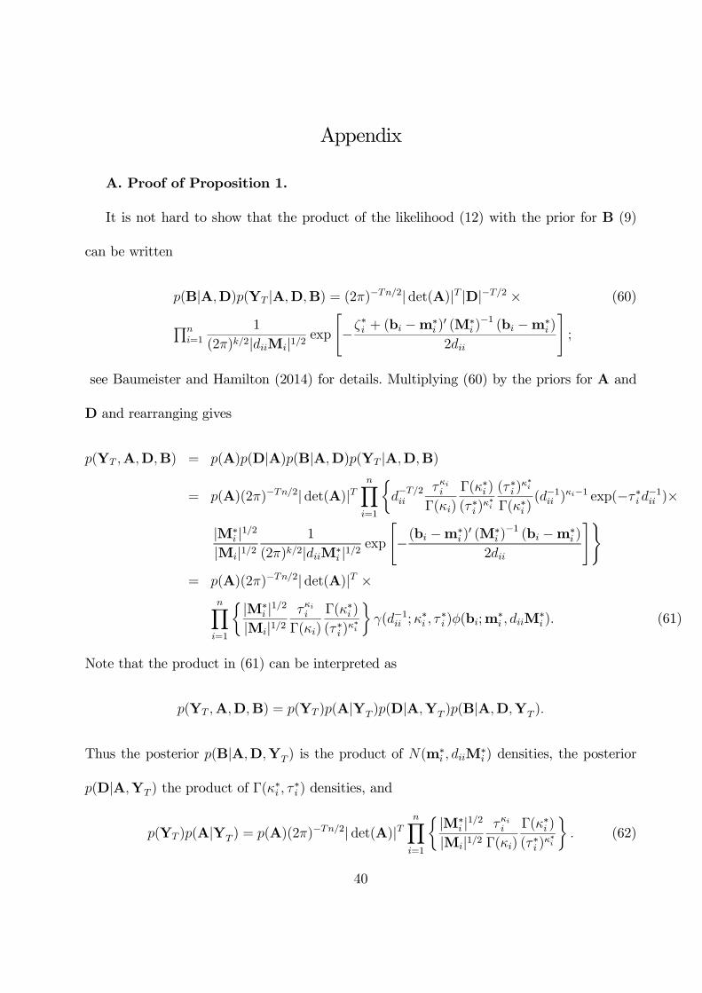
A. Proof of Proposition 1.
It is not hard to show that the product of the likelihood (12) with the prior for B (9)
can be written
p(B|A,D)p(YT |A,D,B) = (2π)−Tn/2|det(A)|T |D|−T/2 × (60)
ni=1
1
(2π)k/2|diiMi|1/2exp
−ζ∗i + (bi −m∗
i )′ (M∗
i )−1 (bi −m∗
i )
2dii
;
see Baumeister and Hamilton (2014) for details. Multiplying (60) by the priors for A and
D and rearranging gives
p(YT ,A,D,B) = p(A)p(D|A)p(B|A,D)p(YT |A,D,B)
= p(A)(2π)−Tn/2|det(A)|Tn
i=1
d−T/2ii
τκiiΓ(κi)
Γ(κ∗i )
(τ ∗i )κ∗i
(τ ∗i )κ∗i
Γ(κ∗i )(d−1ii )κi−1 exp(−τ∗i d−1ii )×
|M∗i |1/2
|Mi|1/21
(2π)k/2|diiM∗i |1/2
exp
−(bi −m∗i )′ (M∗
i )−1 (bi −m∗
i )
2dii
&
= p(A)(2π)−Tn/2|det(A)|T ×n
i=1
|M∗i |1/2
|Mi|1/2τκii
Γ(κi)
Γ(κ∗i )
(τ ∗i )κ∗i
γ(d−1ii ;κ∗i , τ
∗i )φ(bi;m
∗i , diiM
∗i ). (61)
Note that the product in (61) can be interpreted as
p(YT ,A,D,B) = p(YT )p(A|YT )p(D|A,YT )p(B|A,D,YT ).
Thus the posterior p(B|A,D,YT ) is the product of N(m∗i , diiM
∗i ) densities, the posterior
p(D|A,YT ) the product of Γ(κ∗i , τ
∗i ) densities, and
p(YT )p(A|YT ) = p(A)(2π)−Tn/2|det(A)|Tn
i=1
|M∗i |1/2
|Mi|1/2τκii
Γ(κi)
Γ(κ∗i )
(τ∗i )κ∗i
. (62)
40

The posterior p(A|YT ) is thus proportional to (62). Since ΩT is not a function of A, we
can write multiply (62) by |ΩT |T/2 to write the result in an equivalent form that facilitates
numerical calculation and interpretation:
p(A|YT ) ∝p(A)[det(AΩTA
′)]T/2
ni=1[(2τ
∗i /T )]
κ∗i
n
i=1
|M∗i |1/2
|Mi|1/2τκiiΓ(κi)
Γ(κ∗i )
as claimed in equation (20). Note that we could replace ΩT in the numerator with any
matrix not depending on unknown parameters, with any such replacement simply changing
the definition of kT in (20). Our use of ΩT in the numerator helps the target density (which
omits kT ) behave better numerically for large T , as will be seen in the asymptotic analysis
below.
B. Proof of Proposition 2.
Results (i)-(iii) are relatively straightforward; proofs can be found in Baumeister and
Hamilton (2014).
(iv) We first demonstrate that
Prob[A /∈ Hδ(ΩT )]|YT → 0 ∀δ > 0. (63)
To see this, let pij(A,Ω) denote the row i, column j element of P(A,Ω) for P(A,Ω) the
lower-triangular Cholesky factor P(A,Ω)[P(A,Ω)]′ = AΩA′. Note that
|AΩA′| = p211(A,Ω)p222(A,Ω) · · · p2nn(A,Ω)
a′iΩai = p2i1(A,Ω) + p2i2(A,Ω) + · · ·+ p2ii(A,Ω).
41

Furthermore, ζ∗i , the sum of squared residuals from a regression of Yi on Xi, by construction
is larger than Ta′iΩTai, the SSR from a regression of a′iyt on xt−1. Thus
(2τ ∗i /T ) = (2τ i/T ) + ζ∗i /T
≥ a′iΩTai
=i
j=1[p2ij(A, ΩT )]
2.
But for all A /∈ Hδ(ΩT ), ∃ j∗ < i∗ such thatpi∗j∗(A, ΩT )
2> δ∗ for δ∗ = 2δ/[n(n − 1)]
meaning a′i∗ΩTai∗ > [δ∗+pi∗i∗(A, ΩT )]2 for some i∗ and
ni=1(2τ
∗i /T ) > [p11(A, ΩT ]
2 · · · [δ∗+
pi∗i∗(A, ΩT )]2 · · · [pnn(A, ΩT ]
2. Thus
Prob[A /∈ Hδ(ΩT )|YT ] =
'
A/∈Hδ(ΩT )
kTp(A)[p211(A, ΩT )p222(A, ΩT ) · · · p2nn(A, ΩT )]
T/2
ni=1[(2τ i/T ) + ζ
∗i /T ]
κi [(2τ i/T ) + ζ∗i /T ]T/2
dA
<
'
A/∈Hδ(ΩT )
kTp(A)n
i=1[(2τ i/T ) + (ζ∗i /T )]κi×
[p211(A, ΩT )p222(A, ΩT ) · · · p2nn(A, ΩT )]
T/2
[p211(A, ΩT )] · · · [δ∗ + p2i∗i∗(A, ΩT )] · · · [p2nn(A, ΩT ]T/2
dA
=
'
A/∈Hδ(ΩT )
kTp(A)ni=1[(2τ i/T ) + ζ∗i /T ]
κi
p2i∗i∗(A, ΩT )
δ∗ + p2i∗i∗(A, ΩT )
T/2
dA
which goes to 0 as T →∞.
Note next that
Prob[A /∈ Hδ(Ω0)]|YT = Probn
i=2
i−1j=1 [pij(A,Ω0)]
2 > δ.
But
[pij(A,Ω0)]2 =
pij(A, ΩT ) +
pij(A,Ω0)− pij(A, ΩT )
2
≤ 2pij(A, ΩT )
2+ 2
pij(A,Ω0)− pij(A, ΩT )
2.
42
Hence
Prob[A /∈ Hδ(Ω0)]|YT ≤ Prob[(A1T +A2T ) > δ]|YT
A1T = 2n
i=2
i−1j=1
pij(A, ΩT )
2
A2T = 2n
i=2
i−1j=1
pij(A,Ω0)− pij(A, ΩT )
2.
Given any ε > 0 and δ > 0, by virtue of (63) and result (ii) of Proposition 2, there exists a
T0 such that Prob[A1T > δ/2]|YT < ε/2 and Prob[A2T > δ/2]|YT < ε/2 for all T ≥ T0,
establishing that Prob[(A1T +A2T ) > δ]|YT < ε as claimed.
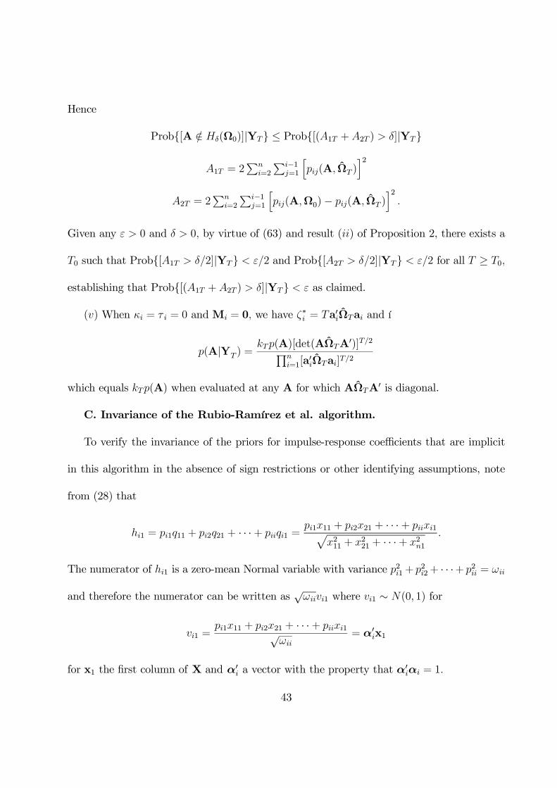
(v) When κi = τ i = 0 and Mi = 0, we have ζ∗i = Ta′iΩTai and í
p(A|YT ) =kTp(A)[det(AΩTA
′)]T/2
ni=1[a
′iΩTai]T/2
which equals kTp(A) when evaluated at any A for which AΩTA′ is diagonal.
C. Invariance of the Rubio-Ramírez et al. algorithm.
To verify the invariance of the priors for impulse-response coefficients that are implicit
in this algorithm in the absence of sign restrictions or other identifying assumptions, note
from (28) that
hi1 = pi1q11 + pi2q21 + · · ·+ piiqi1 =pi1x11 + pi2x21 + · · ·+ piixi1
x211 + x221 + · · ·+ x2n1.
The numerator of hi1 is a zero-mean Normal variable with variance p2i1+ p2i2+ · · ·+ p2ii = ωii
and therefore the numerator can be written as√ωiivi1 where vi1 ∼ N(0, 1) for
vi1 =pi1x11 + pi2x21 + · · ·+ piixi1√
ωii= α′ix1
for x1 the first column of X and α′i a vector with the property that α′iαi = 1.
43

If we then consider the square of the impact, h2i1 = ωiiv2i1/(x
211 + x221 + · · · + x2n1), the
claim is that this is ωii times a Beta(1/2,(n−1)/2) random variable. This would be the case
provided that we can write the denominator as
x211 + x221 + · · ·+ x2n1 = v211 + v221 + · · ·+ v2n1
where (v11, ...., vn1) are independentN(0, 1) and the ith term vi1 is the same term as appears in
the numerator. That this is indeed the case can be verified by noting that since x1 ∼ N(0, In),
it is also the case that v1 ∼ N(0, In) when v1 = αx1 and α is any orthogonal (n×n) matrix.
We can start with any arbitrary unit-length vector α′i for the ith row of α and always fill
in the other rows α′1,α′2, ...,α
′i−1,α
′i+1, ...,α
′n so as to find such an orthogonal matrix α.
Then v′1v1 = x′1α′αx1 = x′1x1 as claimed.
44

References
Akerlof, George A., and William T. Dickens (2007). "Unfinished Business in the Macro-
economics of Low Inflation: A Tribute to George and Bill by Bill and George," Brookings
Papers on Economic Activity 2: 31-47.
Baumeister, Christiane, and James D. Hamilton (2014). "Sign Restrictions, Structural
Vector Autoregressions, and Useful Prior Information," NBER Working Paper No. 20741.
Blanchard, Olivier J. and Peter Diamond (1990). "The Cyclical Behavior of Gross Flows
of Workers in the United States," Brookings Papers on Economic Activity 1990(2): 85-155.
Blanchard, Olivier J., and Danny Quah (1989). "The Dynamic Effects of Aggregate
Demand and Supply Disturbances," American Economic Review 79: 655-673.
Caldara, Dario and Christophe Kamps (2012). "The Analytics of SVARs: A Unified
Framework to Measure Fiscal Multipliers," working paper, Federal Reserve Board.
Canova, Fabio, and Gianni De Nicoló (2002). "Monetary Disturbances Matter for Busi-
ness Fluctuations in the G-7," Journal of Monetary Economics 49: 1131-1159.
Canova, Fabio, and Matthias Paustian (2011). "Business Cycle Measurement with Some
Theory," Journal of Monetary Economics 58: 345-361.
Chetty, Raj, Adam Guren, Day Manoli, and Andrea Weber (2013). "Does Indivisible
Labor Explain the Difference between Micro and Macro Elasticities? A Meta-Analysis of
Extensive Margin Elasticities," NBER Macroeconomics Annual, Volume 27, pp. 1-55, edited
by Daron Acemoglu, Jonathan Parker, and Michael Woodford. Chicago, IL: University of
Chicago Press.
45

Cho, Jang-Ok, and Thomas F. Cooley (1994). "Employment and Hours over the Business
Cycle," Journal of Economic Dynamics and Control 18(2): 411-432.
Datta, Gauri Sankar and Malay Ghosh (1996). "On the Invariance of Noninformative
Priors," Annals of Statistics 24(1): 141-159.
Davis, Steven J. and John Haltiwanger (1999). "On the Driving Forces Behind Cyclical
Movements in Employment and Job Reallocation," American Economic Review 89: 1234-
1258.
Doan, Thomas, Robert B. Litterman, and Christopher A. Sims (1984). "Forecasting and
Conditional Projection Using Realistic Prior Distributions," Econometric Reviews 3: 1-100.
Doan, Thomas (2013). RATS User’s Guide, Version 8.2, www.estima.com.
Devroye, Luc (1986). Non-Uniform Random Variate Generation. Springer-Verlag.
Faust, Jon (1998). "The Robustness of Identified VAR Conclusions about Money,"
Carnegie-Rochester Series on Public Policy 49: 207-244.
Faust, Jon and Eric M. Leeper (1997). "When Do Long-Run Identifying Restrictions
Give Reliable Results?," Journal of Business & Economic Statistics 15: 345-353.
Fry, Renée, and Adrian Pagan (2011). "Sign Restrictions in Structural Vector Autore-
gressions: A Critical Review," Journal of Economic Literature 49(4): 938-960.
Galí, Jordi (1999). "Technology, Employment, and the Business Cycle: Do Technology
Shocks Explain Aggregate Fluctuations?", American Economic Review 89: 249-271.
Galí, Jordi, Frank Smets, and Rafael Wouters (2012). "Unemployment in an Estimated
New Keynesian Model," NBER Macroeconomics Annual, Volume 26, pp. 329-360, edited by
46

Daron Acemoglu, and Michael Woodford. Chicago, IL: University of Chicago Press.
Giacomini, Raffaella, and Toru Kitagawa (2014). "Inference about Non-Identified SVARs,"
working paper, University College London.
Gubner, John A. (2006). Probability and Random Processes for Electrical and Computer
Engineers. Cambridge: Cambridge University Press.
Gustafson, Paul (2009). "What Are the Limits of Posterior Distributions Arising From
Nonidentified Models, and Why Should We Care?", Journal of the American Statistical
Asociation 104: 1682-1695.
Haar, Alfred (1933). "Der Massbegriff in der Theorie der kontinuierlichen Gruppen",
Annals of Mathematics second series 34(1): 147—169.
Hamermesh, Daniel S. (1996). Labor Demand. Princeton: Princeton University Press.
Hamilton, James D. (1994). Time Series Analysis. Princeton: Princeton University
Press.
Kilian, Lutz, and Daniel P. Murphy (2012). "Why Agnostic Sign Restrictions Are Not
Enough: Understanding the Dynamics of Oil Market VAR Models," Journal of the European
Economic Association 10(5): 1166-1188.
Kydland, Finn E., and Edward C. Prescott (1982). "Time to Build and Aggregate
Fluctuations," Econometrica 50(6): 1345-1370.
Leamer, Edward E. (1978). Specification Searches: Ad Hoc Inference with Nonexperi-
mental Data. New York: John Wiley & Sons, Inc.
47
Leamer, Edward E. (1981). "Is it a Demand Curve, Or Is It A Supply Curve? Partial
Identification through Inequality Constraints," Review of Economics and Statistics 63: 319-
327.
Lichter, Andreas, Andreas Peichl, and Sebastian Siegloch (2014). "The Own-Wage Elas-
ticity of Labor Demand: A Meta-Regression Analysis," working paper, Institute for the
Study of Labor.
Litterman, Robert B. (1986). "Forecasting With Bayesian Vector Autoregressions— Five
Years of Experience," Journal of Business & Economic Statistics 4:25-38.
Manski, Charles F. (2003). Partial Identification of Probability Distributions, New York:
Springer.
Moon, Hyungsik Roger, and Frank Schorfheide (2012). "Bayesian and Frequentist Infer-
ence in Partially Identified Models," Econometrica 80: 755-782.
Moon, Hyungsik Roger, Frank Schorfheide, and Eleonora Granziera (2013). "Inference
for VARs Identified with Sign Restrictions", working paper, University of Pennsylvania.
Poirier, Dale J. (1998). "Revising Beliefs in Nonidentified Models," Econometric Theory,
14: 483-509.
Reichling, Felix, and Charles Whalen (2012). "Review of Estimates of the Frisch Elas-
ticity of Labor Supply," working paper, Congressional Budget Office.
Rubio-Ramírez, Juan, Daniel F. Waggoner, and Tao Zha (2010). "Structural Vector
Autoregressions: Theory of Identification and Algorithms for Inference", Review of Economic
Studies, 77(2): 665-696.
48
Shapiro, Matthew D., and Mark W. Watson (1988). "Sources of Business Cycle Fluctu-
ations," NBER Macroeconomics Annual, Volume 3, pp. 111-156, edited by Stanley Fischer.
Cambridge, MA: M.I.T. Press.
Sims, Christopher A., and Tao Zha (1998). "Bayesian Methods for Dynamic Multivariate
Models," International Economic Review 39: 949-968.
Tamer, Elie (2010). "Partial Identification in Econometrics," Annual Review of Eco-
nomics 2: 167-195.
Theil, Henri (1971). Principles of Econometrics. New York: John Wiley & Sons, Inc.
Uhlig, Harald (2005). "What are the Effects of Monetary Policy on Output? Results
from an Agnostic Identification Procedure," Journal of Monetary Economics 52: 381—419.
49

50
Figure 1. Prior densities for initial effect of shocks implicit in traditional approach to sign-restricted VAR.
Panel A: response of variable i to one-standard-deviation increase of any structural shock when number
of variables in VAR is 2 (solid blue) or 6 (dashed green). Panel B: response of variable i to a structural
shock that increases variable j by one unit.
00
1
2
3
-ωii1/2 ωii
1/2
n = 6
n = 2
Panel A
hij
0
0.1
0.2
0.3
0.4
ωij / ωjj
Panel B
hij*
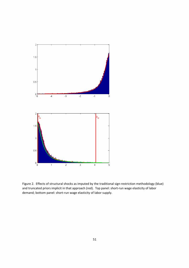
51
Figure 2. Effects of structural shocks as imputed by the traditional sign-restriction methodology (blue)
and truncated priors implicit in that approach (red). Top panel: short-run wage elasticity of labor
demand; bottom panel: short-run wage elasticity of labor supply.

52
Figure 3. Prior densities when a uniform prior is used for the effect of shock 1 and number of variables
is 2. Panel A: prior density for response of variable 1 to structural shock 1. Panel B: prior density for
response of variable 1 to structural shock 2.

53
Figure 4. Maximum likelihood estimates and likelihood contours for α and β. Distance between contour
lines is 10, and unshaded regions are exceedingly unlikely given the data.
-5 -4 -3 -2 -1 0 1 2 3 4 5-5
0
5The function β(α)
hHhL
β
α
β
α
Contours for log likelihood
hH
-5 -4 -3 -2 -1 0 1 2 3 4 5-5
0
5
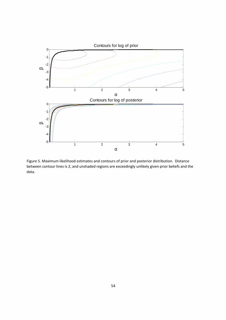
54
Figure 5. Maximum likelihood estimates and contours of prior and posterior distribution. Distance
between contour lines is 2, and unshaded regions are exceedingly unlikely given prior beliefs and the
data.
β
α
Contours for log of prior
1 2 3 4 5-5
-4
-3
-2
-1
0
β
α
Contours for log of posterior
1 2 3 4 5-5
-4
-3
-2
-1
0

55
Figure 6. Distributions for prior (red curves) and posterior (blue histograms). Panel A: short-run
elasticity of labor demand; panel B: short-run elasticity of labor supply; panel C: long-run labor-supply
parameter (negative of lower left element of the matrix in equation (55)).
-3 -2 -1 00
0.5
1β d
0 1 2 30
2
4
6
α s
-0.5 0 0.5 10
2
4
6
α s + b11 s + b
21 s + ... + b
m1 s
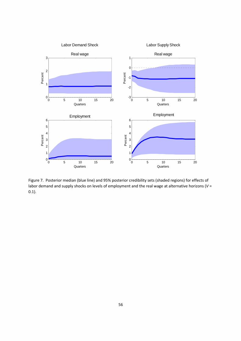
56
Figure 7. Posterior median (blue line) and 95% posterior credibility sets (shaded regions) for effects of
labor demand and supply shocks on levels of employment and the real wage at alternative horizons (V =
0.1).
0 5 10 15 200
1
2
3
Labor Demand Shock
Real wage
Per
cent
Quarters0 5 10 15 20
-3
-2
-1
0
1
Labor Supply Shock
Real wage
Quarters
Per
cent
0 5 10 15 200
1
2
3
4
5
6Employment
Quarters
Per
cent
0 5 10 15 200
1
2
3
4
5
6
Employment
Quarters
Per
cent

57
Figure 8. Effect of stronger priors about the long-run labor supply elasticity. Left column: response of
employment to a labor demand shock for prior weights given by V = 1, 0.1, 0.01, or 0.001; right column:
distribution for short-run labor supply elasticity for prior (red curve) and posterior (blue histograms)
associated with different values of V.
0 0.2 0.4 0.6 0.8 10
5
10
α s
V = 1
0 5 10 15 200
2
4
6
Response of employment to labor demand shock
V = 1
Per
cent
0 0.2 0.4 0.6 0.8 10
5
10
V = 0.1
0 5 10 15 200
2
4
6V = 0.1
Per
cent
0 0.2 0.4 0.6 0.8 10
5
10
V = 0.01
0 5 10 15 200
2
4
6V = 0.01
Per
cent
0 0.2 0.4 0.6 0.8 10
5
10
V = 0.001
0 5 10 15 200
2
4
6V = 0.001
Quarters
Per
cent


