SIGGRAPH 2007 Course Notes / Materials

SIGGRAPH 2007 Course Notes / Materials Submission Sample Guidelines Course Notes Sample • Sample

− The course notes sample concisely demonstrates proposed published content for course proposal review

• Simple − The course notes sample only needs to be long enough to evaluate anticipated quality.

Recommended length: 12-18 pages. Overly long submissions will not necessarily improve reviews.

• Sufficient − Reviewers will evaluate content for aspects such as clarity, visual quality, topic

development and detail, ease of use, etc. • Complete

− In addition to the course notes sample, please outline any additional resources to be published with the course notes (such as animation files, source code, bibliographies, web resources, etc.)

Submission Checklist • Samples should be submitted in Portable Document Format (PDF).

− Important for uniform support of reviewers across many platforms. • The excerpt should demonstrate development of a significant topic or theme from the

syllabus. − If the course notes originate from your presentation slides, consider providing speaker

annotations where a slide might require additional explanatory details. − Individual presenters may each provide a brief excerpt of their work as part of the review

sample. − SIGGRAPH 2007 presentation slide templates are available on the SIGGRAPH 2007 web

site. • Provide a summary page of any additional materials intended for publication (images, video,

source code, web sources, etc.) as a supplementary reference. Past Examples • The attached examples demonstrate the qualities of highly regarded course note samples

− Henrik Wann Jensen: A Practical Guide to Global Illumination with Ray Tracing and Photon Mapping

− Ebert, et. al.: The Elements of Nature: Interactive and Realistic Techniques − Shreiner, et. al.: An Interactive Introduction to OpenGL Programming − Note: any one example would be sufficient for submission review

• Excellent PDF course note examples can also be referenced on the DVDs and CD-ROMs from past conferences (SIGGRAPH 1996 through 2006 – available from http://store.acm.org/acmstore/)

A Practical Guide toGlobal Illumination using

Ray Tracingand

Photon Mapping

Siggraph 2002 Course 19

Monday, August 9, 2004

Organizer & Lecturer

Henrik Wann JensenUniversity of California, San Diego

Abstract

This course serves as a practical guide to ray tracing and photon map-

ping. The notes are mostly aimed at readers familiar with ray tracing,

who would like to add an efficient implementation of photon mapping

to an existing ray tracer. The course itself also includes a description

of the ray tracing algorithm.

There are many reasons to augment a ray tracer with photon maps.

Photon maps makes it possible to efficiently compute global illumina-

tion including caustics, diffuse color bleeding, and participating me-

dia. Photon maps can be used in scenes containing many complex

objects of general type (i.e. the method is not restricted to tessellated

models). The method is capable of handling advanced material de-

scriptions based on a mixture of specular, diffuse, and non-diffuse

components. Furthermore, the method is easy to implement and ex-

periment with.

This course is structured as a half day course. We will therefore as-

sume that the participants have knowledge of global illumination al-

gorithms (in particular ray tracing), material models, and radiometric

terms such as radiance and flux. We will discuss in detail photon trac-

ing, the photon map data structure, the photon map radiance estimate,

and rendering techniques based on photon maps. We will emphasize

the techniques for efficient computation throughout the presentation.

Finally, we will present several examples of scenes rendered with pho-

ton maps and explain the important aspects that we considered when

rendering each scene.

About the Lecturer

Henrik Wann Jensen

University of California, San [email protected]://graphics.ucsd.edu/˜henrik

Dr. Henrik Wann Jensen is an assistant professor at the University of California atSan Diego, where he is establishing a computer graphics lab. with a research fo-cus on realistic image synthesis, global illumination, rendering of natural phenom-ena, and appearance modeling. His contributions to computer graphics include thephoton mapping algorithm for global illumination, and the first technique for effi-ciently simulating subsurface scattering in translucent materials. He is the authorof ”Realistic Image Synthesis using Photon Mapping,” AK Peters 2001. Prior tocoming to UCSD in 2002, he was a research associate at Stanford University from1999-2002, a postdoctoral researcher at the Massachusetts Institute of Technology(MIT) from 1998-1999, and a research scientist in industry working on commercialrendering software from 1996-1998. He received his M.Sc. and Ph.D. in ComputerScience from the Technical University of Denmark in 1996 for developing the pho-ton mapping method.In 2004, Professor Jensen received an Academy Award (Technical AchievementAward) from the Academy of Motion Picture Arts and Sciences for pioneeringresearch in rendering translucent materials, and he became a Sloan Fellow.

Course Overview

1 minutes: Introduction and WelcomeHenrik Wann Jensen

Overview of the course and motivation for attending it.

19 minutes: The Ray Tracing AlgorithmHenrik Wann Jensen

This part will cover the basics of the ray tracing algorithm.

35 minutes: Photon Tracing: Building the Photon MapsHenrik Wann Jensen

This part of the course will cover efficient techniques for photon tracingincluding:

• Emitting photons from the light sources in the scene

• The use of projection maps

• Simulating scattering and absorption of photons using Russian Roulette

• Storing photons in the photon map

• Preparing the photon map for rendering

Also the use of several photon maps for the simulation of caustics, soft indi-rect illumination and participating media will be described.

45 minutes: Rendering using Photon MappingHenrik Wann Jensen

This part will cover the details of how to integrate photon mapping into a raytracer, and how to use it for rendering of 3D models.

Several examples will be shown to illustrate the various aspects of the com-bination of ray tracing and photon mapping.

Contents

1 Introduction 71.1 Motivation . . . . . . . . . . . . . . . . . . . . . . . . . . . . . . 71.2 What is photon mapping? . . . . . . . . . . . . . . . . . . . . . . 81.3 Overview of the course material . . . . . . . . . . . . . . . . . . 91.4 More information . . . . . . . . . . . . . . . . . . . . . . . . . . 91.5 Acknowledgements . . . . . . . . . . . . . . . . . . . . . . . . . 10

Part 1: Henrik Wann Jensen 11

2 A Practical Guide to Global Illumination using Photon Mapping 112.1 Photon tracing . . . . . . . . . . . . . . . . . . . . . . . . . . . . 11

2.1.1 Photon emission . . . . . . . . . . . . . . . . . . . . . . 112.1.2 Photon tracing . . . . . . . . . . . . . . . . . . . . . . . 152.1.3 Photon storing . . . . . . . . . . . . . . . . . . . . . . . 182.1.4 Extension to participating media . . . . . . . . . . . . . . 202.1.5 Three photon maps . . . . . . . . . . . . . . . . . . . . . 22

2.2 Preparing the photon map for rendering . . . . . . . . . . . . . . 222.2.1 The balanced kd-tree . . . . . . . . . . . . . . . . . . . . 232.2.2 Balancing . . . . . . . . . . . . . . . . . . . . . . . . . . 24

2.3 The radiance estimate . . . . . . . . . . . . . . . . . . . . . . . . 252.3.1 Radiance estimate at a surface . . . . . . . . . . . . . . . 252.3.2 Filtering . . . . . . . . . . . . . . . . . . . . . . . . . . . 282.3.3 The radiance estimate in a participating medium . . . . . 302.3.4 Locating the nearest photons . . . . . . . . . . . . . . . . 30

2.4 Rendering . . . . . . . . . . . . . . . . . . . . . . . . . . . . . . 332.4.1 Direct illumination . . . . . . . . . . . . . . . . . . . . . 352.4.2 Specular and glossy reflection . . . . . . . . . . . . . . . 36

5

2.4.3 Caustics . . . . . . . . . . . . . . . . . . . . . . . . . . . 372.4.4 Multiple diffuse reflections . . . . . . . . . . . . . . . . . 382.4.5 Participating media . . . . . . . . . . . . . . . . . . . . . 392.4.6 Why distribution ray tracing? . . . . . . . . . . . . . . . 39

2.5 Examples . . . . . . . . . . . . . . . . . . . . . . . . . . . . . . 412.5.1 The Cornell box . . . . . . . . . . . . . . . . . . . . . . 412.5.2 Cornell box with water . . . . . . . . . . . . . . . . . . . 472.5.3 Fractal Cornell box . . . . . . . . . . . . . . . . . . . . . 482.5.4 Cornell box with multiple lights . . . . . . . . . . . . . . 492.5.5 Cornell box with smoke . . . . . . . . . . . . . . . . . . 502.5.6 Cognac glass . . . . . . . . . . . . . . . . . . . . . . . . 512.5.7 Prism with dispersion . . . . . . . . . . . . . . . . . . . . 522.5.8 Subsurface scattering . . . . . . . . . . . . . . . . . . . . 53

2.6 Where to get programs with photon maps . . . . . . . . . . . . . 54

3 References and further reading 57

6

Chapter 1

Introduction

This course material describes in detail the practical aspects of the photon mapalgorithm. The text is based on previously published papers, technical reports anddissertations (in particular [Jensen96c]). It also reflects the experience obtainedwith the implementation of the photon map as it was developed at the TechnicalUniversity of Denmark. After reading this course material, it should be relativelystraightforward to add an efficient implementation of the photon map algorithm toany ray tracer.

1.1 Motivation

The photon mapping method is an extension of ray tracing. In 1989, AndrewGlassner wrote about ray tracing [Glassner89]:

“Today ray tracing is one of the most popular and powerful tech-niques in the image synthesis repertoire: it is simple, elegant, and eas-ily implemented. [However] there are some aspects of the real worldthat ray tracing doesn’t handle very well (or at all!) as of this writ-ing. Perhaps the most important omissions are diffuse inter-reflections(e.g. the ‘bleeding’ of colored light from a dull red file cabinet onto awhite carpet, giving the carpet a pink tint), and caustics (focused light,like the shimmering waves at the bottom of a swimming pool).”

At the time of the development of the photon map algorithm in 1993, these prob-lems were still not addressed efficiently by any ray tracing algorithm. The pho-ton map method offers a solution to both problems. Diffuse interreflections and

7

caustics are both indirect illumination of diffuse surfaces; with the photon mapmethod, such illumination is estimated using precomputed photon maps. Extend-ing ray tracing with photon maps yields a method capable of efficiently simulatingall types of direct and indirect illumination. Furthermore, the photon map methodcan handle participating media and it is fairly simple to parallelize [Jensen00].

1.2 What is photon mapping?

The photon map algorithm was developed in 1993–1994 and the first papers on themethod were published in 1995. It is a versatile algorithm capable of simulatingglobal illumination including caustics, diffuse interreflections, and participatingmedia in complex scenes. It provides the same flexibility as general Monte Carloray tracing methods using only a fraction of the computation time.

The global illumination algorithm based on photon maps is a two-pass method.The first pass builds the photon map by emitting photons from the light sources intothe scene and storing them in aphoton mapwhen they hit non-specular objects.The second pass, the rendering pass, uses statistical techniques on the photon mapto extract information about incoming flux and reflected radiance at any point inthe scene. The photon map is decoupled from the geometric representation of thescene. This is a key feature of the algorithm, making it capable of simulatingglobal illumination in complex scenes containing millions of triangles, instancedgeometry, and complex procedurally defined objects.

Compared with finite element radiosity, photon maps have the advantage thatno meshing is required. The radiosity algorithm is faster for simple diffuse scenesbut as the complexity of the scene increases, photon maps tend to scale better. Alsothe photon map method handles non-diffuse surfaces and caustics.

Monte Carlo ray tracing methods such as path tracing, bidirectional path trac-ing, and Metropolis can simulate all global illumination effects in complex sceneswith very little memory overhead. The main benefit of the photon map comparedwith these methods is efficiency, and the price paid is the extra memory used tostore the photons. For most scenes the photon map algorithm is significantly faster,and the result looks better since the error in the photon map method is of low fre-quency which is less noticeable than the high frequency noise of general MonteCarlo methods.

Another big advantage of photon maps (from a commercial point of view) isthat there is no patent on the method; anyone can add photon maps to their renderer.

8

As a result several commercial systems use photon maps for rendering caustics andglobal illumination.

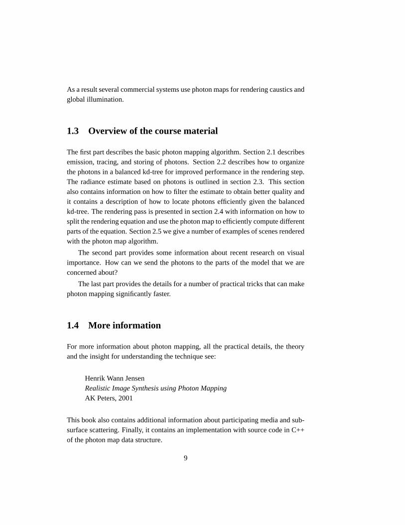
1.3 Overview of the course material

The first part describes the basic photon mapping algorithm. Section 2.1 describesemission, tracing, and storing of photons. Section 2.2 describes how to organizethe photons in a balanced kd-tree for improved performance in the rendering step.The radiance estimate based on photons is outlined in section 2.3. This sectionalso contains information on how to filter the estimate to obtain better quality andit contains a description of how to locate photons efficiently given the balancedkd-tree. The rendering pass is presented in section 2.4 with information on how tosplit the rendering equation and use the photon map to efficiently compute differentparts of the equation. Section 2.5 we give a number of examples of scenes renderedwith the photon map algorithm.

The second part provides some information about recent research on visualimportance. How can we send the photons to the parts of the model that we areconcerned about?

The last part provides the details for a number of practical tricks that can makephoton mapping significantly faster.

1.4 More information

For more information about photon mapping, all the practical details, the theoryand the insight for understanding the technique see:

Henrik Wann JensenRealistic Image Synthesis using Photon MappingAK Peters, 2001

This book also contains additional information about participating media and sub-surface scattering. Finally, it contains an implementation with source code in C++of the photon map data structure.

9

1.5 Acknowledgements

The inspiration behind this course is Alan Chalmers. Without his suggestion (overa beer) this course might never have materialized. Thanks, Alan! Thanks to PerChristensen, Frank Suykens, and Toshi Kato for participating in previous versionsof the course. In addition, thanks to Niels Jørgen Christensen, Martin Blais, By-ong Mok Oh, Gernot Schaufler and Maryann Simmons for helpful comments onthe notes. Finally, thanks to intellectual property counsel Karen Hersey at Mas-sachusetts Institute of Technology.

10

Chapter 2

A Practical Guide to GlobalIllumination using PhotonMapping

2.1 Photon tracing

The purpose of the photon tracing pass is to compute indirect illumination on dif-fuse surfaces. This is done by emitting photons from the light sources, tracing themthrough the scene, and storing them at diffuse surfaces.

2.1.1 Photon emission

This section describes how photons are emitted from a single light source and frommultiple light sources, and describes the use of projection maps which can increasethe emission efficiency considerably.

Emission from a single light source

The photons emitted from a light source should have a distribution correspondingto the distribution of emissive power of the light source. This ensures that theemitted photons carry the same flux — ie. we do not waste computational resourceson photons with low power.

Photons from a diffuse point light source are emitted in uniformly distributedrandom directions from the point. Photons from a directional light are all emittedin the same direction, but from origins outside the scene. Photons from a diffuse

11

square light source are emitted from random positions on the square, with direc-tions limited to a hemisphere. The emission directions are chosen from a cosinedistribution: there is zero probability of a photon being emitted in the directionparallel to the plane of the square, and highest probability of emission is in thedirection perpendicular to the square.

In general, the light source can have any shape and emission characteristics —the intensity of the emitted light varies with both origin and direction. For example,a (matte) light bulb has a nontrivial shape and the intensity of the light emittedfrom it varies with both position and direction. The photon emission should followthis variation, so in general, the probability of emission varies depending on theposition on the surface of the light source and the direction.

��

��

Figure 2.1: Emission from light sources: (a) point light, (b) directional light,(c) square light, (d) general light.

Figure 2.1 shows the emission from these different types of light sources.

The power (“wattage”) of the light source has to be distributed among the pho-tons emitted from it. If the power of the light isPlight and the number of emittedphotons isne, the power of each emitted photon is

Pphoton =Plight

ne. (2.1)

Pseudocode for a simple example of photon emission from a diffuse point lightsource is given in Figure 2.2.

To further reduce variation in the computed indirect illumination (during ren-dering), it is desirable that the photons are emitted as evenly as possible. This canfor example be done with stratification [Rubinstein81] or by using low-discrepancyquasi-random sampling [Keller96].

12

emit photons from diffuse point light() {ne = 0 number of emitted photonswhile (not enough photons) {

do { use simple rejection sampling to find diffuse photon directionx = random number between -1 and 1y = random number between -1 and 1z = random number between -1 and 1

} while ( x2 + y2 + z2 > 1 )

~d = < x, y, z >~p = light source position

trace photon from ~p in direction ~dne = ne + 1

}scale power of stored photons with 1/ne

}

Figure 2.2: Pseudocode for emission of photons from a diffuse point light

Multiple lights

If the scene contains multiple light sources, photons should be emitted from eachlight source. More photons should be emitted from brighter lights than from dimlights, to make the power of all emitted photons approximately even. (The infor-mation in the photon map is best utilized if the power of the stored photons isapproximately even). One might worry that scenes with many light sources wouldrequire many more photons to be emitted than scenes with a single light source.Fortunately, it is not so. In a scene with many light sources, each light contributesless to the overall illumination, and typically fewer photons can be emitted fromeach light. If, however, only a few light sources are important one might use animportance sampling map [Peter98] to concentrate the photons in the areas that areof interest to the observer. The tricky part about using an importance map is that wedo not want to generate photons with energy levels that are too different since thiswill require a larger number of photons in the radiance estimate (see section 2.3)to ensure good quality.

13

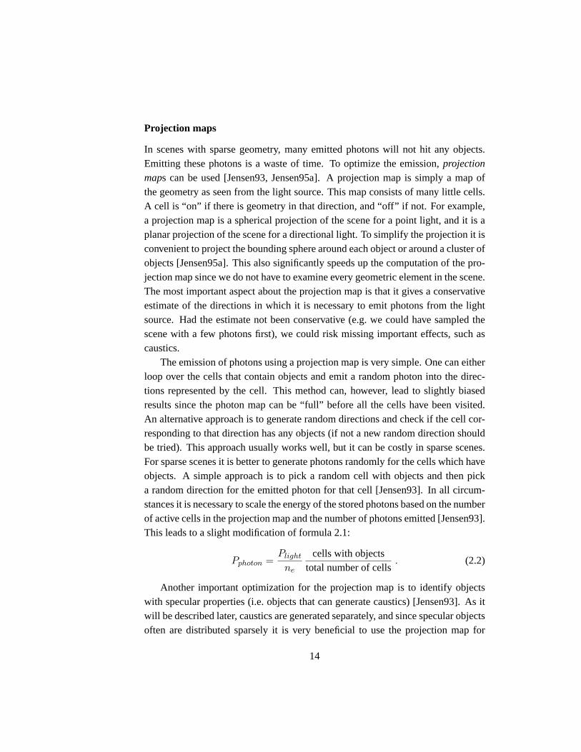
Projection maps

In scenes with sparse geometry, many emitted photons will not hit any objects.Emitting these photons is a waste of time. To optimize the emission,projectionmaps can be used [Jensen93, Jensen95a]. A projection map is simply a map ofthe geometry as seen from the light source. This map consists of many little cells.A cell is “on” if there is geometry in that direction, and “off” if not. For example,a projection map is a spherical projection of the scene for a point light, and it is aplanar projection of the scene for a directional light. To simplify the projection it isconvenient to project the bounding sphere around each object or around a cluster ofobjects [Jensen95a]. This also significantly speeds up the computation of the pro-jection map since we do not have to examine every geometric element in the scene.The most important aspect about the projection map is that it gives a conservativeestimate of the directions in which it is necessary to emit photons from the lightsource. Had the estimate not been conservative (e.g. we could have sampled thescene with a few photons first), we could risk missing important effects, such ascaustics.

The emission of photons using a projection map is very simple. One can eitherloop over the cells that contain objects and emit a random photon into the direc-tions represented by the cell. This method can, however, lead to slightly biasedresults since the photon map can be “full” before all the cells have been visited.An alternative approach is to generate random directions and check if the cell cor-responding to that direction has any objects (if not a new random direction shouldbe tried). This approach usually works well, but it can be costly in sparse scenes.For sparse scenes it is better to generate photons randomly for the cells which haveobjects. A simple approach is to pick a random cell with objects and then picka random direction for the emitted photon for that cell [Jensen93]. In all circum-stances it is necessary to scale the energy of the stored photons based on the numberof active cells in the projection map and the number of photons emitted [Jensen93].This leads to a slight modification of formula 2.1:

Pphoton =Plight

ne

cells with objectstotal number of cells

. (2.2)

Another important optimization for the projection map is to identify objectswith specular properties (i.e. objects that can generate caustics) [Jensen93]. As itwill be described later, caustics are generated separately, and since specular objectsoften are distributed sparsely it is very beneficial to use the projection map for

14

caustics.

2.1.2 Photon tracing

Once a photon has been emitted, it is traced through the scene using photon tracing(also known as “light ray tracing”, “backward ray tracing”, “forward ray tracing”,and “backward path tracing”). Photon tracing works in exactly the same way as raytracing except for the fact that photons propagate flux whereas rays gather radiance.This is an important distinction since the interaction of a photon with a material canbe different than the interaction of a ray. A notable example is refraction whereradiance is changed based on the relative index of refraction[Hall88] — this doesnot happen to photons.

When a photon hits an object, it can either be reflected, transmitted, or ab-sorbed. Whether it is reflected, transmitted, or absorbed is decided probabilisticallybased on the material parameters of the surface. The technique used to decide thetype of interaction is known as Russian roulette [Arvo90] — basically we roll adice and decide whether the photon should survive and be allowed to perform an-other photon tracing step.

Examples of photon paths are shown in Figure 2.3.

Reflection, transmission, or absorption?

For a simple example, we first consider a monochromatic simulation. For a re-flective surface with a diffuse reflection coefficientd and specular reflection coeffi-cients (with d + s ≤ 1) we use a uniformly distributed random variableξ ∈ [0, 1](computed with for exampledrand48()) and make the following decision:

ξ ∈ [0, d] −→ diffuse reflectionξ ∈]d, s + d] −→ specular reflectionξ ∈]s + d, 1] −→ absorption

In this simple example, the use of Russian roulette means that we do not have tomodify the power of the reflected photon — the correctness is ensured by averagingseveral photon interactions over time. Consider for example a surface that reflects50% of the incoming light. With Russian roulette only half of the incoming photonswill be reflected, but with full energy. For example, if you shoot 1000 photons atthe surface, you can either reflect 1000 photons with half the energy or 500 photonswith full energy. It can be seen that Russian roulette is a powerful technique forreducing the computational requirements for photon tracing.

15

a

bc

Figure 2.3: Photon paths in a scene (a “Cornell box” with a chrome sphere on leftand a glass sphere on right): (a) two diffuse reflections followed by absorption, (b) aspecular reflection followed by two diffuse reflections, (c) two specular transmissionsfollowed by absorption.

With more color bands (for example RGB colors), the decision gets slightlymore complicated. Consider again a surface with some diffuse reflection and somespecular reflection, but this time with different reflection coefficients in the threecolor bands. The probabilities for specular and diffuse reflection can be based onthe total energy reflected by each type of reflection or on the maximum energyreflected in any color band. If we base the decision on maximum energy, we canfor example compute the probabilityPd for diffuse reflection as

Pd =max(drPr, dgPg, dbPb)

max(Pr, Pg, Pb)

where(dr, dg, db) are the diffuse reflection coefficients in the red, green, and bluecolor bands, and(Pr, Pg, Pb) are the powers of the incident photon in the samethree color bands.

Similarly, the probabilityPs for specular reflection is

Ps =max(srPr, sgPg, sbPb)

max(Pr, Pg, Pb)

where(sr, sg, sb) are the specular reflection coefficients.

16

The probability of absorbtion isPa = 1 − Pd − Ps. With these probabilities,the decision of which type of reflection or absorption should be chosen takes thefollowing form:

ξ ∈ [0, Pd] −→ diffuse reflectionξ ∈]Pd, Ps + Pd] −→ specular reflectionξ ∈]Ps + Pd, 1] −→ absorption

The power of the reflected photon needs to be adjusted to account for the proba-bility of survival. If, for example, specular reflection was chosen in the exampleabove, the powerPrefl of the reflected photon is:

Prefl,r = Pinc,r sr/Ps

Prefl,g = Pinc,g sg/Ps

Prefl,b = Pinc,b sb/Ps

wherePinc is the power of the incident photon.The computed probabilities again ensure us that we do not waste time emitting

photons with very low power.It is simple to extend the selection scheme to also handle transmission, to han-

dle more than three color bands, and to handle other reflection types (for exampleglossy and directional diffuse).

Why Russian roulette?

Why do we go through this effort to decide what to do with a photon? Why not justtrace new photons in the diffuse and specular directions and scale the photon energyaccordingly? There are two main reasons why the use of Russian roulette is a verygood idea. Firstly, we prefer photons with similar power in the photon map. Thismakes the radiance estimate much better using only a few photons. Secondly, ifwe generate, say, two photons per surface interaction then we will have28 photonsafter 8 interactions. This means 256 photons after 8 interactions compared to 1photon coming directly from the light source! Clearly this is not good. We want atleast as many photons that have only 1–2 bounces as photons that have made 5–8bounces. The use of Russian roulette is therefore very important in photon tracing.

There is one caveat with Russian roulette. It increases variance on the solution.Instead of using the exact values for reflection and transmission to scale the photonenergy we now rely on a sampling of these values that will converge to the correctresult as enough photons are used.

17

(a) (b)

Figure 2.4: “Cornell box” with glass and chrome spheres: (a) ray traced image (di-rect illumination and specular reflection and transmission), (b) the photons in thecorresponding photon map.

Details on photon tracing and Russian roulette can be found in [Shirley90,Pattanaik93, Glassner95].

2.1.3 Photon storing

This section describes which photon-surface interactions are stored in the photonmap. It also describes in more detail the photon map data structure.

Which photon-surface interactions are stored?

Photons are only stored where they hit diffuse surfaces (or, more precisely, non-specular surfaces). The reason is that storing photons on specular surfaces doesnot give any useful information: the probability of having a matching incomingphoton from the specular direction is zero, so if we want to render accurate specularreflections the best way is to trace a ray in the mirror direction using standard raytracing. For all other photon-surface interactions, data is stored in a global datastructure, thephoton map. Note that each emitted photon can be stored severaltimes along its path. Also, information about a photon is stored at the surfacewhere it is absorbed if that surface is diffuse.

18

Chapter 3

References and further reading

This section lists the references referenced in these course notes plus additionalbackground material relevant to the photon map method. The material is dividedinto three groups: the photon map method, ray tracing and photon tracing anddata-structures with focus on kd-trees. Each part is in chronological order withannotations. In addition we have listed a number of animations rendered with pho-ton maps and finally we have provided a more detailed list of relevant backgroundliterature.

The photon map method

[Jensen95a] Henrik Wann Jensen and Niels Jørgen Christensen.“Photon maps in Bidirectional Monte Carlo Ray Tracing ofComplex Objects”.Computers & Graphics19 (2), pages 215–224, 1995.The first paper describing the photon map. The paper sug-gested the use of a mixture of photon maps and illuminationmaps, where photon maps would be used for complex surfacessuch as fractals.

[Jensen95b] Henrik Wann Jensen.“Importance driven path tracing using the photon map”.Rendering Techniques ’95 (Proceedings of the Sixth Euro-graphics Workshop on Rendering), pages 326–335. SpringerVerlag, 1995.Introduces the use of photons for importance sampling in path

57

tracing. By combining the knowledge of the incoming fluxwith the BRDF it is possible to get better results using fewersample rays.

[Jensen95c] Henrik Wann Jensen and Niels Jørgen Christensen.“Efficiently Rendering Shadows using the Photon Maps”.In Proceedings of Compugraphics’95, pages 285–291, Alvor,December 1995.Introduces the use of shadow photons for an approximate clas-sification of the light source visibility in a scene.

[Jensen96a] Henrik Wann Jensen.“Rendering caustics on non-Lambertian surfaces”.Proceedings of Graphics Interface’96, pages 116-121,Toronto, May 1996 (also selected for publication in ComputerGraphics Forum, volume 16, number 1, pages 57–64, March1997). Extension of the photon map method to render causticson non-Lambertian surfaces ranging from diffuse to glossy.

[Jensen96b] Henrik Wann Jensen.“Global illumination using photon maps”.Rendering Techniques ’96 (Proceedings of the Seventh Euro-graphics Workshop on Rendering), pages 21–30. Springer Ver-lag, 1996.Presents the global illumination algorithm using photon maps.A caustic and a global photon map is used to optimize the ren-dering of global illumination including the simulation of caus-tics.

[Jensen96c] Henrik Wann Jensen.The photon map in global illumination.Ph.D. dissertation, Technical University of Denmark, Septem-ber 1996.An in-depth description of the photon map method based onthe presentations in the published photon map papers.

[Christensen97] Per H. Christensen.“Global illumination for professional 3D animation, visualiza-tion, and special effects” (invited paper).

58

6-1

Interactive Cloud Modeling and Photorealistic Atmospheric Rendering

David S. Ebert [email protected]

1 Overview In this chapter, I provide an introductory tutorial on basic procedural modeling for simulating clouds in Sections 2-4. Then, a paper by Joshua Schpok, et al. from the Symposium on Computer Animation 2003 is included to show how to adapt these techniques to the latest graphics hardware. Next, I include a paper on accurate illumination from clouds using graphics hardware by Kirk Riley et al. from Visualization 2003 is presented. Finally, a copy of my powerpoint slides are included.

2 An Introduction to Procedural Modeling and Animation As mentioned in the course introduction, we are working in a very exciting time. The combination of increased CPU power with powerful, programmable, graphics processors (GPUs) available on affordable PCs has started an age where we can envision and realize interactive complex procedural models.

This chapter presents a framework for procedural modeling and animation of gaseous phenomena using volumetric procedural models: a general class of procedural techniques for modeling natural phenomena. Volumetric procedural models use three-dimensional volume density functions

6-2

(vdf(x,y,z)) that define the density of a continuous three-dimensional space. Volume density functions (vdf's) are the natural extension of solid texturing [Perlin1985] to describe the actual geometry of objects. Volume density functions are used extensively in computer graphics for modeling and animating gases, fire, fur, liquids, and other "soft'' objects. Hypertextures [Perlin1989] and Inakage's flames [Inakage1991] are other examples of the use of volume density functions.

Many advanced geometric modeling techniques are inherently procedural. L-systems, fractals, particle systems, and implicit surfaces [Bloomenthal1997] (also called blobs and metaballs), are, to some extent, procedural and can be combined nicely into the framework of volumetric procedural models. This chapter will concentrate on the development and animation of several volume density functions for creating realistic images and animations of clouds. The inclusion of fractal techniques into vdf's is presented in most of the examples because they rely on a statistical simulation of turbulence that is fractal in nature. This chapter will also briefly discuss the inclusion of implicit function techniques into vdf's. A more complete discussion of the simulation of noise and turbulence functions, as well as a thorough presentation of procedural modeling and texturing techniques, can be found in Texturing and Modeling: A Procedural Approach, 2nd edition, [Ebert2002]1. This text also contains a thorough discussion of the detailed development of volumetric procedural modeling, which forms a good basis to this chapter.

2.1 Procedural Techniques and Computer Graphics

Procedural techniques have been used throughout the history of computer graphics. Many early modeling and texturing techniques included procedural definitions of geometry and surface color. From these early beginnings, procedural techniques have exploded into an important, powerful modeling, texturing, and animation paradigm. During the mid- to late 1980s, procedural techniques for creating realistic textures, such as marble, wood, stone, and other natural material gained widespread use. These techniques were extended to procedural modeling, including models of water, smoke, steam, fire, planets, and even tribbles. The development of the RenderMan2 shading language [Pixar1989] in 1989 greatly expanded the use of procedural techniques. Currently, most commercial rendering and animation systems even provide a procedural interface. Procedural techniques have become an exciting, vital aspect of creating realistic computer generated images and animations. As the field continues to evolve, the importance and significance of procedural techniques will continue to grow.

2.2 Definition and Power of Procedural Techniques

Procedural techniques are code segments or algorithms that specify some characteristic of a computer generated model or effect. For example, a procedural texture for a marble surface does not use a scanned-in image to define the color values. Instead, it uses algorithms and mathematical functions to determine the color.

1 As of March 1999, two of the co-authors of this book have won Academy Awards for their computer graphics contributions used in motion pictures: Darwyn Peachey and Ken Perlin.

2 RenderMan is a registered trademark of Pixar.

6-3

One of the most important features of procedural techniques is abstraction. In a procedural approach, rather than explicitly specifying and storing all the complex details of a scene or sequence, we abstract them into a function or an algorithm (i.e., a procedure) and evaluate that procedure when and where needed. We gain a storage savings, as the details are no longer explicitly specified but rather implicit in the procedure, and shift the time requirements for specification of details from the programmer to the computer. This allows us to create inherently multi-resolution models and textures that we can evaluate to the resolution needed.

We also gain the power of parametric control, allowing us to assign to a parameter a meaningful concept (e.g., a number that makes mountains "rougher'' or "smoother''). Parametric control also provides amplification of the modeler/animator's efforts: a few parameters yield large amounts of detail (Smith [Smith1984] referred to this as database amplification). This parametric control unburdens the user from the low-level control and specification of detail. We also gain the serendipity inherent in procedural techniques: we are often pleasantly surprised by the unexpected behaviors of procedures, particularly stochastic procedures. Procedural models also offer flexibility. The designer of the procedures can capture the essence of the object, phenomenon, or motion without being constrained by the complex laws of physics. Procedural techniques allow the inclusion of any amount of physical accuracy into the model that is desired. The designer may produce a wide range of effects, from accurately simulating natural laws to purely artistic effects.

2.3 Background

The techniques described in this chapter use procedurally defined volume density functions for modeling, texturing, and animating gases. There have been numerous previous approaches to modeling gases in computer graphics, including Kajiya's simple physical approximation [Kajiya1984], Gardner's solid textured ellipsoids [Gardner1985, Gardner1990], Max's height fields [Max1986], constant density media [Klassen1987, Nishita1987], and fractals [Voss1983]. I have developed several approaches for modeling and controlling the animation of gases [Ebert 1989, Ebert1990a, Ebert1990b, Ebert1991, Ebert1992]. Stam has used "fuzzy blobbies'' as a three-dimensional model for animating gases [Stam1993] and has extended their use to modeling fire [Stam1995].

Volume rendering is essential for realistic images and animations of gases. Any procedure-based volume rendering system, such as Perlin's [Perlin1989], or my system [Ebert1990a, Ebert1991], can be used for rendering volumetric procedural models. A volume ray-tracer is also very easy to extend to allow the support of procedural volumetric modeling. My system is a hybrid rendering system that uses a fast scanline a-buffer rendering algorithm for the surface-defined objects in the scene, while volume modeled objects are volume rendered. This rendering system features a physically-based low-albedo illumination and atmospheric attenuation model for the gases. Volumetric shadows are also efficiently combined into the system through the use of three-dimensional shadow tables [Ebert1990a, Ebert2002]. Precomputing these procedures at a fixed resolution 3D grid defeats many of the advantages of the procedural model, but allows these to be loaded as 3D textures into the latest PC and workstation boards and enables interactive rendering and exploration of these procedural models. PC graphics boards are now available with 3D texture mapping hardware, which enables interactive or even real-time volume rendering with precomputed volumetric models. Additionally, 3D texture mapping is part of the DirectX 8.0 standard and the OpenGL 1.2 standard, so we should expect to find this feature on all high-end PC

6-4

graphics boards shortly.

3 Volumetric Cloud Modeling with Implicit Functions Modeling clouds is a very difficult task because of their complex, amorphous structure and because even an untrained eye can judge the realism of a cloud model. Their ubiquitous nature makes them an important modeling and animation task. This chapter describes a new volumetric procedural approach for cloud modeling and animation that allows easy, natural specification and animation of the clouds, flexibility to include as much physics or art as desired into the model, unburdens the user from detailed geometry specification, and produces realistic volumetric cloud models. This technique combines the flexibility of volumetric procedural modeling with the smooth blending and ease of control of primitive-based implicit functions (metaballs, blobs) to create a powerful new modeling technique. This technique also demonstrates the advantages of primitive-based implicit functions for modeling semi-transparent volumetric objects.

3.1 Background

Modeling clouds in computer graphics has been a challenge for over twenty years [Dungan1979] and major advances in cloud modeling still warrant presentation in the SIGGRAPH Papers Program (e.g., [Dobashi2000]). Many previous approaches have used semi-transparent surfaces to produce convincing images of clouds [Gardner1984, Gardner1985, Gardner1990, Voss1983]. Although these techniques can produce realistic images of clouds viewed from a distance, these cloud models are hollow and do not allow the user to seamlessly enter, travel through, and inspect the interior of the cloud model. To capture the three-dimensional structure of a cloud, volumetric density-based models must be used. Kajiya [Kajiya1984] produced the first volumetric cloud model in computer graphics, but the results are not photo-realistic. Stam [Stam1995], Foster [Foster1997], and Ebert [Ebert1994] have produced convincing volumetric models of smoke and steam, but have not done substantial work on modeling clouds. Neyret [Neyret1997] has recently produced some preliminary results of a convective cloud model based on general physical characteristics. This model may be promising for simulating convective clouds; however, it currently uses surfaces (large particles) to model the cloud structure. A general, flexible, easy-to-use, realistic volumetric cloud model is still needed in computer graphics.

In developing this new cloud modeling and animation system, I have chosen to build upon the recent work in advanced modeling techniques and volumetric procedural modeling. Many advanced geometric modeling techniques, such as fractals [Peitgen1992], implicit surfaces [Blinn1982, Wyvill1986, Nishimura1985], grammar-based modeling [Smith1984, Prusinkiewicz1990], and volumetric procedural models/hypertextures [Perlin1985, Ebert1994] use procedural abstraction of detail to allow the designer to control and animate objects at a high level. Their inherent procedural nature provides flexibility, data amplification, abstraction of detail, and ease of parametric control. When modeling complex volumetric phenomena, such as clouds, this abstraction of detail and data amplification are necessary to make the modeling and animation tractable. It would be impractical for an animator to specify and control the detailed three-dimensional density of a cloud model. This system does not use a physics-based approach because it is computationally prohibitive and non-intuitive to use for many animators and modelers. Setting and animating correct physics parameters for dew point, particulate distributions, temperature and pressure gradients, etc. is a time-consuming, detailed task. This model was developed to allow the

6-5

modeler and animator to work at a much higher level. I also didn't want to restrict the results by the laws of physics, but to allow for artistic expression.

Volumetric procedural models have all of the advantages of procedural techniques and are a natural choice for cloud modeling because they are the most flexible advanced modeling technique. Since a procedure is evaluated to determine the object's density, any advanced modeling technique, simple physics simulation, mathematical function or artistic algorithm can be included in the model.

Combining traditional volumetric procedural models with implicit functions creates a model that has the advantages of both techniques. Implicit functions have been used for many years as a modeling tool for creating solid objects and smoothly blended surfaces [Bloomenthal1997]. However, little work has been done to explore their potential for modeling volumetric density distributions of semi-transparent volumes. Nishita [Nishita1996] has used volume rendered implicits as a basic cloud model in his work on multiple scattering illumination models; however, this work has concentrated on illumination effects and not on realistic modeling of the cloud geometry. Stam has also used volumetric blobbies to create his models of smoke and clouds [Stam1991, Stam1993, Stam1995]. His work is related to the approach described in this chapter. My early work on using volume rendered implicit spheres to produce a fly-through of a volumetric cloud was described in [Ebert1997a]. This work has been developed further to use implicits to provide a natural way of specifying and animating the global structure of the cloud, while using more traditional procedural techniques to model the detailed structure.

3.2 Volumetric Procedural Modeling With Implicit Functions

The volumetric cloud model uses a two-level: the cloud macrostructure and the cloud microstructure. Implicit functions and turbulent volume densities model these, respectively. The basic structure of the cloud model combines these two components to determine the final density of the cloud.

The cloud's microstructure is created by using procedural turbulence and noise functions, in a manner similar to my basic_gas function (see [Ebert2002]). This allows the procedural simulation of natural detail to the level needed. Simple mathematical functions are added to allow shaping of the density distributions and control over the sharpness of the density falloff.

Implicit functions were chosen to model the cloud macrostructure because of their ease of specification and smoothly blending density distributions. The user simply specifies the location, type, and weight of the implicit primitives to create the overall cloud shape. Any implicit primitive, including spheres, cylinders, ellipsoids, and skeletal implicits can be used to model the cloud macrostructure. Since these are volume rendered as a semi-transparent medium, the whole volumetric field function is being rendered, as compared to implicit surface rendering where only a small range of values of the field are used to create the objects. The implicit density functions are primitive-based density functions: they are defined by summed, weighted, parameterized, primitive implicit surfaces. A simple example of the implicit formulation of a sphere centered at the point center with radius r is the following:

F(x,y,z): (x - center.x)2 + (y-center.y) 2 + (z-center.z) 2 - r2 = 0.

The real power of implicit functions is the smooth blending of the density fields from separate

6-6

primitive sources. I chose to use Wyvill's standard cubic function [Wyvill1986] as the density (blending) function for the implicit primitives:

1922

917

94)( 2

2

4

4

6

6

+−+−=Rr

Rr

RrrFcub .

In the above equation, r is the distance from the primitive. This density function is a cubic in the distance squared and its value ranges from 1 when r=0 (within the primitive) to 0 at r=R. This density function has several advantages. First, its value drops off quickly to zero (at the distance R), reducing the number of primitives that must be considered in creating the final surface. Second, it has zero derivatives at r=0 and r=R and is symmetrical about the contour value 0.5, providing for smooth blends between primitives. The final implicit density value is then the weighted sum of the density field values of each primitive:

))(()( qpFwpDensityicub

iiimplicit −= ∑

where wi is the weight of the ith primitive and q is the closest point on element i from p.

To create non-solid implicit primitives, the location of the point is procedurally altered before the evaluation of the blending functions. This alteration can be the product of the procedure and the implicit function and/or a warping of the implicit space.

These techniques are combined into a simple cloud model as shown below: volumetric_procedural_implicit_function(pnt, blend%, pixel_size) perturbed_point = procedurally alter pnt using noise and turbulence density1 = implicit_function(perturbed_point) density2 = turbulence(pnt, pixel_size) blend = blend% * density1 +(1 - blend%) * density2 density = shape resulting density based on user controls for wispiness and denseness(e.g., use pow & exponential function) return(density)

The density from the implicit primitives is combined with a pure turbulence based density using a user specified blend% (60% to 80% gives good results). The blending of the two densities allows the creation of clouds that range from entirely determined by the implicit function density to entirely determined by the procedural turbulence function. When the clouds are completely determined by the implicit functions, they will tend to look more like cotton balls. The addition of the procedural alteration and turbulence is what gives them their naturalistic look.

3.3 Volumetric Cloud Modeling

The volumetric procedural implicit algorithm given above forms the basis of a flexible system for the modeling of volumetric objects. This chapter focuses on the use of these techniques for modeling and animating realistic clouds. The volume rendering of the clouds is not discussed in detail. For a description of the volume rendering system that was used to make my images of clouds in this book, please see [Ebert1990a, Ebert2002]. Any volume rendering system can be used with these volumetric cloud procedures; however, to get realistic effects, the system should accumulate densities using atmospheric attenuation, and a physics-based illumination algorithm

6-7

should be used. For accurate images of cumulus clouds, a high-albedo illumination algorithm (e.g., [Max1994, Nishita1996]) is needed.

3.3.1 Cumulus Clouds

Cumulus clouds are very common in nature and can be easily simulated using spherical or elliptical implicit primitives. Figure 1 shows the type of result that can be achieved by using nine implicit spheres to model a cumulus cloud. The animator/modeler simply positions the implicit spheres to produce the general cloud structure. Procedural modification then alters the density distribution to create the detailed wisps. The algorithm used to create the clouds in Figure 1 is the following:

cumulus(pnt,density,parms, pnt_w, vol) xyz_td pnt; /* location of point in cloud space */ xyz_td pnt_w; /* location of point in world space */ float *density,*parms; vol_td vol; { float new_turbulence(); /* my turbulence function */ float peachey_noise(); /* Darwyn Peachey's noise function */ float metaball_evaluate(); /* function for evaluating the metaball primitives*/ float mdens, /* metaball density value */ turb, /* turbulence amount */ peach; /* Peachey noise value */ xyz_td path; /* path for swirling the point */ extern int frame_num; static int ncalcd=1; static float sin_theta_cloud, cos_theta_cloud, theta, path_x, path_y, path_z, scalar_x, scalar_y, scalar_z; /* calculate values that only depend on the frame number once per frame */ if(ncalcd) { ncalcd=0; /* create gentle swirling in the cloud */ theta =(frame_num%600)*01047196; /* swirling effect */ cos_theta_cloud = cos(theta); sin_theta_cloud = sin(theta); path_x = sin_theta_cloud*.005*frame_num; path_y = .01215*(float)frame_num; path_z= sin_theta_cloud*.0035*frame_num; scalar_x = (.5+(float)frame_num*0.010); scalar_z = (float)frame_num*.0073; } /* Add some noise to the point's location */ peach = peachey_noise(pnt); /* Use Darwyn Peachey's noise function */ pnt.x -= path_x -peach*scalar_x; pnt.y = pnt.y - path_y +.5*peach; pnt.z += path_z - peach*scalar_z; /* Perturb the location of the point before evaluating the implicit primitives. */ turb=fast_turbulence(pnt); turb_amount=parms[4]*turb; pnt_w.x += turb_amount; pnt_w.y -= turb_amount; pnt_w.z += turb_amount; mdens=(float)metaball_evaluate((double)pnt_w.x, (double)pnt_w.y, (double)pnt_w.z, (vol.metaball)); *density= parms[1]*(parms[3]*mdens + (1.0 - parms[3])*turb*mdens); *density= pow(*density,(double)parms[2]); }

6-8

Parms[3] is the blending function value between implicit (metaball) density and the product of the turbulence density and the implicit density. This method of blending ensures that the entire cloud density is a product of the implicit field values, preventing cloud pieces from occurring outside the defining primitives. Using a large parms[3] generates clouds that are mainly defined by their implicit primitives and are, therefore, ``smoother'' and less turbulent. Parms[1] is a density scaling factor, parms[2] is the exponent for the pow() function, and parms[4] controls the amount of turbulence to use in displacing the point before evaluation of the implicit primitives. For good images of cumulus clouds, useful values are the following: 0.2 < parms[1] < 0.4, parms[2] = 0.5, parms[3]=0.4, and parms[4] = 0.7 .

3.3.2 Cirrus and Stratus Clouds

Cirrus clouds differ greatly from cumulus clouds in their density, thickness, and falloff. In general, cirrus clouds are thinner, less dense, and wispier. These effects can be created by altering the parameters to the cumulus cloud procedure and also by changing the implicit primitives. The density value parameter for a cirrus cloud is normally chosen as a smaller value and the exponent is chosen larger, producing larger areas of no clouds and a greater number of individual clouds. To create cirrus clouds, the user can simply specify the global shape (envelope) of the clouds with a few implicit primitives or specify implicit primitives to determine the location and shape of each cloud. In the former case, the shape of each cloud is mainly controlled by the volumetric procedural function and turbulence simulation, as opposed to cumulus clouds where the implicit functions are the main shape control. It is also useful to modulate the densities along the direction

Figure 1: An example of a cumulus cloud. Copyright 2001 David S. Ebert

6-9

of the jet stream to produce more natural wisps. This can be created by the user specifying a predominant direction of wind flow and using a turbulent version of this vector in controlling the densities as follows:

Cirrus(pnt,density,parms, pnt_w, vol, jet_stream) xyz_td pnt; /* location of point in cloud space */ xyz_td pnt_w; /* location of point in world space */ xyz_td jet_stream; float *density,*parms; vol_td vol; { float new_turbulence(); /* my turbulence function */ float peachey_noise(); /* Darwyn Peachey's noise function */ float metaball_evaluate(); /* function for evaluating the metaball primitives*/ float mdens, /* metaball density value */ turb, /* turbulence amount */ peach; /* Peachey noise value */ xyz_td path; /* path for swirling the point */ extern int frame_num; static int ncalcd=1; static float sin_theta_cloud, cos_theta_cloud, theta, path_x, path_y, path_z, scalar_x, scalar_y, scalar_z; /* calculate values that only depend on the frame number once per frame */ if(ncalcd) { ncalcd=0; /* create gentle swirling in the cloud */ theta =(frame_num%600)*01047196; /* swirling effect */ cos_theta_cloud = cos(theta); sin_theta_cloud = sin(theta); path_x = sin_theta_cloud*.005*frame_num; path_y = .01215*(float)frame_num; path_z= sin_theta_cloud*.0035*frame_num; scalar_x = (.5+(float)frame_num*0.010); scalar_z = (float)frame_num*.0073; } /* Add some noise to the point's location */ peach = peachey_noise(pnt); /* Use Darwyn Peachey's noise function */ pnt.x -= path_x -peach*scalar_x; pnt.y = pnt.y - path_y +.5*peach; pnt.z += path_z - peach*scalar_z; /* Perturb the location of the point before evaluating the implicit * primitives.*/ turb=fast_turbulence(pnt); turb_amount=parms[4]*turb; pnt_w.x += turb_amount; pnt_w.y -= turb_amount; pnt_w.z += turb_amount; /* make the jet stream turbulent */ jet_stream.x + =.2*turb; jet_stream.y + =.3*turb; jet_stream.z + =.25*turb; /* warp point along the jet stream vector */ pnt_w = warp(jet_stream, pnt_w); mdens=(float)metaball_evaluate((double)pnt_w.x, (double)pnt_w.y, (double)pnt_w.z, (vol.metaball)); *density= parms[1]*(parms[3]*mdens + (1.0 - parms[3])*turb*mdens); *density= pow(*density,(double)parms[2]); }

6-10

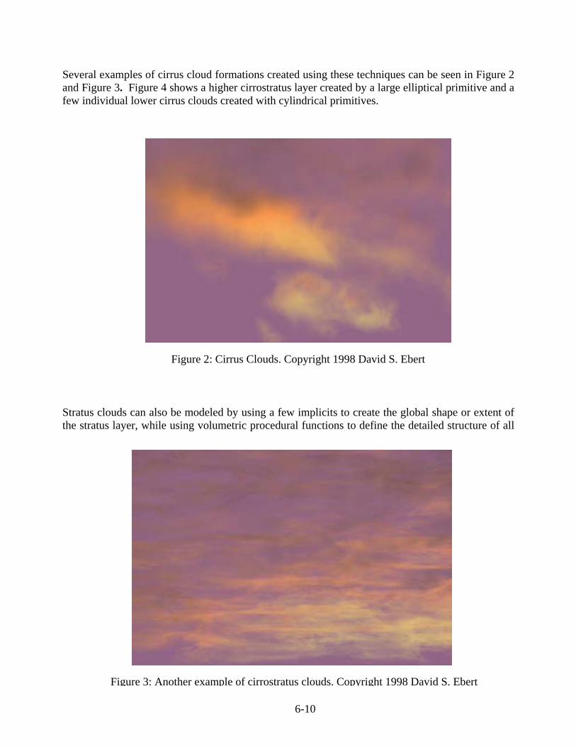
Several examples of cirrus cloud formations created using these techniques can be seen in Figure 2 and Figure 3. Figure 4 shows a higher cirrostratus layer created by a large elliptical primitive and a few individual lower cirrus clouds created with cylindrical primitives.

Stratus clouds can also be modeled by using a few implicits to create the global shape or extent of the stratus layer, while using volumetric procedural functions to define the detailed structure of all

Figure 2: Cirrus Clouds. Copyright 1998 David S. Ebert

Figure 3: Another example of cirrostratus clouds. Copyright 1998 David S. Ebert

6-11

of the clouds within this layer. Stratus cloud layers are normally thicker and less wispy, as compared with cirrus clouds. This effect can be created by adjusting the size of the turbulent space (smaller/fewer wisps), using a smaller exponent value (creates more of a cloud layer effect), and increasing the density of the cloud. Using simple mathematical functions to shape the densities can create some of the more interesting stratus effects, such as a mackerel sky. The mackerel stratus cloud layer in Figure 4 was created by modulating the densities with turbulent sine waves in the x and y directions.

3.3.3 User Specification and Control

Since the system uses implicit primitives for the cloud macrostructure, the user creates the general cloud structure by specifying the location, type, and weight of each implicit primitive. For the image in Figure 1, nine implicit spheres were positioned to create the cumulus cloud. Figure 2 shows the wide range of cloud shapes and creatures that can be created by simply adjusting the location of each primitive and the overall density of the model through a simple GUI. The use of implicit primitives makes this a much more natural interface than with traditional procedural techniques. Each of the cloud models in this chapter was created in less than 30 minutes of design time.

The user of the system also specifies a density scaling factor, a power exponent for the density distribution (controls amount of wispiness), any warping procedures to apply, and the name of the volumetric procedural function so that special effects can be programmed into the system.

Figure 4: A mackerel stratus cloud layer. Copyright 1998 David S. Ebert

6-12

3.4 Animating Volumetric Procedural Clouds

The volumetric cloud models described above produce nice still images of clouds and also clouds that gently evolve over time. The models can be animated using the procedural animation techniques described in [Ebert1991, Ebert2002] or by animating the implicit primitives. Procedural animation is the most flexible and powerful technique since any deformation, warp or physical simulation can be added to the procedure. An animator ca use key frames or dynamics simulations to animate the implicit primitives. Several examples of applying these two animation techniques for various effects are described below.

3.4.1 Procedural Animation

Both the implicit primitives and the procedural cloud space can be animated algorithmically. One of most useful forms of implicit primitive animation is warping. A time varying warp function can be used to gradually warp the shape of the cloud over time to simulate the formation of clouds, their movement, and their deformation by wind and other forces. Cloud formations are usually altered based on the jet stream. To simulate this effect, all that is needed is to warp the primitives along a vector representing the jet stream. This can be done by warping the points before evaluating the implicit functions. The amount of warping can be controlled by the wind velocity, or gradually added in over time to simulate the initial cloud development. Implicits can be warped along the jet stream as follows:

perturb_pnt = procedurally alter pnt using noise and turbulence height = relative height of perturb_pnt vector = jet_stream + turbulence(pnt) perturb_pnt = warp(perturb_pnt, vector, height) density1 = implicit_function(perturbed_pnt)

...

To get more natural effects, it is useful to alter each point by a small amount of turbulence before warping it. Several frames from an animation of a cumulus cloud warping along the jet stream can be seen in Figure 5. To create this effect, ease-in and ease-out based on the frame number was used to animate the warp amount. The implicit primitives' locations do not move in this animation, but

Figure 5: Example cloud warping. Copyright 1998 David S. Ebert

6-13

the warping function animates the space to move and distort the cloud along the jet stream vector. Other warping functions to simulate squash and stretch [Bloomenthal1997] and other effects can also be used. Instead of a single vector and velocity, a vector field is input into the program to define more complex weather patterns. The current system allows the specification of vector flow tables and tables of functional primitives (attractors, vortices) to control the motion and deformation of the clouds. This procedural warping technique was used successfully by Stam in animating gases [Stam1995].

3.4.2 Implicit Primitive Animation

The implicit primitives can be animated in the same manner as implicit surfaces: each primitive's location, parameters (e.g., radii), and weight can be animated over time. This provides an easy to use high-level animation interface for cloud animation. This technique was used in the animation, "A Cloud is Born,'' [Ebert1997b] showing the birth of a cumulus cloud followed by a fly-through of it. Several stills from the formation sequence can be seen Figure 6. For this animation, the centers of the implicit spheres were moved over time to simulate three separate cloud elements merging and growing into a full cumulus cloud. The radii of the spheres were also increased over time. Finally, to create animation in the detailed cloud structure, each point was moved along a turbulent path over time before evaluation of the turbulence function, as illustrated in the cumulus procedure. A powerful animation tool for volumetric procedural implicit functions is the use of dynamics and physics-based simulations to control the movement of the implicits and the deformation of space.

Figure 6: Several stills from "A Cloud is Born." Copyright 1997 David S. Ebert

6-14

Since the implicits are modeling the macro-structure of the cloud while procedural techniques are modeling the microstructure, fewer primitives are needed to achieve complex cloud models. Dynamics simulations can be applied to the clouds by using particle system techniques, with each particle representing a volumetric implicit primitive. The smooth blending and procedurally generated detail allow complex results with less than a few hundred primitives, a factor of 100 to 1000 less than needed with traditional particle systems. I have implemented a simple particle system for volumetric procedural implicit particles. The user specifies a few initial implicit primitives, dynamics information, such as speed, initial velocity, force function, and lifetime, and the system generates the location, number, size, and type of implicit for each frame. In our initial tests, it took less than 1 minute to generate and animate the implicit particles for 200 frames. Unlike traditional particle systems, cloud implicit particles never die, they just become dormant. Cumulus clouds created through this volumetric procedural implicit particle system can be seen in Figure 7. The stills in Figure 7 show a cloud created by an upward turbulent force. The number of children created from a particle was also controlled by the turbulence of the particle's location. For the animations in this figure, the initial number of implicit primitives was 12 and the final number was approximately 50.

The animation and formation of cirrus and stratus clouds can also be controlled by the use of a volumetric procedural implicit particle system. For the formation of a large area of cirrus or cirrostratus clouds, the particle system can randomly seed space and then use turbulence to grow the clouds from the creation of new implicit primitives, as can be seen in Figure 8. The cirrostratus layer in this image contains 150 implicit primitives, which were generated from the user specifying 5 seed primitives.

Figure 7: Formation of a cumulus cloud using a volumetric procedural implicit

particle system. Copyright 1998 David S. Ebert

6-15

To control the dynamics of the cloud particle system, any commercial particle animation program can also be used. A useful approach for cloud dynamics is to use qualitative dynamics: simple simulations of the observed properties and formation of clouds. The underlying physical forces that create a wide range of cloud formations are extremely complex to simulate, computationally expensive, and very restrictive. The incorporation of simple, parameterized rules that simulate observable cloud behavior will produce a powerful cloud animation system.

4 Interactivity and Clouds

4.1 Simple Interactive Cloud Models

There are several physical processes that govern the formation of clouds. Simple visual simulations of these techniques with particle systems can be used to get more convincing cloud formation animations. Neyret [Neyret97] suggested that the following physical processes are important to cloud formation simulations:

• Rayleigh Taylor instability: Rayleigh-Taylor instabilities result when a heavy fluid is supported by a less dense fluid against the force of gravity. Any perturbation along the interface between the two fluids will grow.

• Bubbles: a small globule of gas in a thin liquid envelope.

Figure 8: Cirrostratus cloud layer formation using a volumetric procedural

implicit particle system. Copyright 1998 David S. Ebert

6-16

• Rate variation of Temperature. • Kelvin -Helmholtz instability: instability associated with airflows having marked

vertical shear and weak thermal stratification. The common name for this instability is Kelvin-Helmholtz instability. These instabilities are often visualized as a row of horizontal eddies aligned within this layer of vertical shear.

• Vortices: A measure of the local rotation in a fluid flow. In weather analysis and forecasting, it usually refers to the vertical component of rotation.

• Bernard Cells: the hexagonal shaped convection eddies that can form in a solution that is being heated.

Neyret's model takes into account three phenomena at various scales: hot spot generation on the ground, simulation of bubbles rising bubble and reaching their dew point, bubble creation and evolution inside the cloud and their emergence as turrets on the borders. His proposed model incorporates:

• Bubble Generation - rising of hot air parcels due to buoyancy force caused by difference in density. Compute attraction force among parcels. Threshold of energy required for rising. Once it rises, fresh air takes its place and its probability to rise again decreases - emulates "Bernard Cell" behavior.

• Cloud evolution - the cloud is composed of static bubbles. The birth of a bubble inside the cloud is due to the local temperature gradient (Rayleigh Taylor instability).

• Direction of bubble depends on the local heat gradient. • Small scale shape - it assumes a recursive structure for the small scale shape of the

cloud. A bubble is considered as a sphere onto which are convected the main vortices, which were initially waves. The vortices are also assumed to be spherical and sub vortices are advected upon their parent vortex surface in a recursive fashion.

4.2 Rendering Clouds in Commercial Packages

The main component needed to effectively render clouds is volume rendering support in your renderer. Volumetric shadows, low- or high-albedo illumination and correct atmospheric attenuation are needed to get realistic looking clouds. An example of a volume rendering plug-in for Maya that can used to created volume rendered clouds can be found on the Maya Conductor CD from 1999 and on the HighEnd3D web page http://www.highend3d.com/maya/plugins . The plug-in, volumeGas, by Marlin Rowley and Vlad Korolov, implements a simplified version of my volume renderer (which was used to produce the images in these notes).

4.3 Interactive Rendering and Interaction with Procedural Clouds on PC Hardware

With the prevelance of programmable hardware graphics pipelines, what are the important factors for generating true, interactive procedural models of natural phenomena? The following are several important factors that must be considered:

1. How much programmability is needed and available at the following levels: • Vertex

6-17

• Fragment 2. Precision of the programmable operations:

• Are these 8-bit quantities? 9-bit? 12-bit? • Are they fixed range (e.g., 0 to 1)? • What precision is needed to not produce artifacts?

3. What mathematical operations are available? • More advanced operations (sqrt, sin, cos, etc.)?

4. Are dependent operations allowed (can the results of one operation change the next computation)?

5. How efficient is execution of conditionals, branching, looping constructs?

All of the above factors greatly affect the type of procedural models that can be implemented at interactive rates. Current hardware allows flexible programmability of the GPU and we can create interactive procedural models. However, the operations that are available at the fragment level are somewhat limited and the precision for semi-transparent volumes can be is a serious limiting factor. The ability to compute a result at the fragment level and use this to change a texture coordinate used in the next texture look-up is a basic capability that is now available and enables basic procedural solid texturing, etc. Unfortunately, to create amazing, complex procedural models in real-time we need the ability to generate new geometry at the fragment level. We could then download to the GPU a small procedural model that creates geometry representing our procedural model in real-time. This is a feature that probably won’t be available for several years. But, with clever programming, we can create some very interesting, advanced procedural effects with the programmability available in the latest graphics boards.

5 References [Blinn1982] Blinn, J., "Light Reflection Functions for Simulation of Clouds and Dusty Surfaces," Computer Graphics

(SIGGRAPH '82 Proceedings), 16(3)21:29, July 1982.

[Bloomenthal1997] Bloomenthal, J., Bajaj, C., Blinn, J., Cani-Gascuel, M.P., Rockwood, A., Wyvill, B., Wyvill, G., Introduction to Implicit Surfaces, Morgan Kaufman Publishers, 1997.

[Dungan1979] Dungan, W. Jr., "A Terrain and Cloud Computer Image Generation Model," Computer Graphics (SIGGRAPH 85 Proceedings), 19:41-44, July 1985.

[Dobashi2000] Yoshinori Dobashi and Kazufumi Kaneda and Hideo Yamashita and Tsuyoshi Okita and Tomoyuki Nishita. A Simple, Efficient Method for Realistic Animation of Clouds, Proceedings of SIGGRAPH 2000, Computer Graphics Proceedings, Annual Conference Series, pp. 19-28 (July 2000). ACM Press / ACM SIGGRAPH / Addison Wesley Longman. Edited by Kurt Akeley. ISBN 1-58113-208-5.

[Ebert1989] Ebert, D., Boyer, K., Roble, D., "Once a Pawn a Foggy Knight…," [videotape], SIGGRAPH Video Review, 54. ACM SIGGRAPH, 1989.

[Ebert1990a] Ebert, D. and Parent, R., "Rendering and Animation of Gaseous Phenomena by Combining Fast Volume and Scanline A-buffer Techniques." Computer Graphics (SIGGRAPH 90 Conference Proceedings), 24:357-366, August 1990.

[Ebert1990b] Ebert, D., Ebert, J., and Boyer, K., "Getting Into Art" [videotape], Department of Computer and Information Science, The Ohio State University, May1990.

[Ebert1991] Ebert, D., Solid Spaces: A Unified Approach to Describing Object Attributes. Ph.D. Thesis, The Ohio State University, 1991.

6-18

[Ebert1994] Ebert, D., Carlson, W., Parent, R., "Solid Spaces and Inverse Particle Systems for Controlling the Animation of Gases and Fluids," The Visual Computer, 10(4):179-190, 1994.

[Ebert1997a] Ebert, D., "Volumetric Modeling with Implicit Functions: A Cloud is Born," SIGGRAPH 97 Visual Proceedings (Technical Sketch), 147, ACM SIGGRAPH 1997.

[Ebert1997b] Ebert, D., Kukla, J., Bedwell, T., Wrights, S., "A Cloud is Born," ACM SIGGRAPH Video Review (SIGGRAPH 97 Electronic Theatre Program), ACM SIGGRAPH, August 1997.

[Ebert2002] Ebert, D., Musgrave, F., Peachey, D., Perlin, K., Worley, S., Texturing and Modeling: A Procedural Approach, Third Edition, Morgan Kaufman, 2002.

[Foster1997] Foster, N., Metaxas, D., "Modeling the Motion of Hot Turbulent Gases," SIGGRAPH 97 Conference Proceedings, ACM SIGGRAPH 1997.

[Gardner1984] Gardner, G., "Simulation of Natural Scenes Using Textured Quadric Surfaces," Computer Graphics (SIGGRAPH '84 Conference Proceedings), 18, July 1984.

[Gardner1985] Gardner, G., "Visual Simulation of Clouds," Computer Graphics (SIGGRAPH '85 Conference Proceedings), 19(3), July 1985.

[Gardner1990] Gardner, G., "Forest Fire Simulation," Computer Graphics (SIGGRAPH 90 Conference Proceedings), 24, August 1990.

[Inakage1991] Inakage, M., "Modeling Laminar Flames," SIGGRAPH 91 Course Notes 27, ACM SIGGRAPH, July 1991.

[Kajiya1984] Kajiya, J., von Herzen, B., "Ray Tracing Volume Densities," Computer Graphics (SIGGRAPH '84 Conference Proceedings), 18, July 1984.

[Kajiya1989] Kajiya, J., Kay, T., "Rendering Fur with Three-dimensional Textures," Computer Graphics (SIGGRAPH 89 Conference Proceedings), 23, July 1989.

[Max1986] Max, N., "Light Diffusion Through Clouds and Haze," Computer Vision, Graphics, and Image Processing, 33(3), March 1986.

[Max1994] Max, N., "Efficient Light Propagation for Multiple Anisotropic Volume Scattering," Fifth Eurographics Workshop on Rendering, June 1994.

[Neyret1997] Neyret, F., "Qualitative Simulation of Convective Cloud Formation and Evolution," Eight International Workshop on Computer Animation and Simulation, Eurographics, September 1997.

[Nishimura1985] Nishimura, H., Hirai, A., Kawai, T., Kawata, T., Shirakawa, I., Omura, K., "Object Modeling by Distribution Function and a Method of Image Generation," Journal of Papers Given at the Electronics Communication Conference '85, J68-D(4), 1985.

[Nishita1987] Nishita, T., Miyawaki, Y., Nakamae, E., "A shading model for atmospheric scattering considering luminous intensity distribution of light sources," Computer Graphics (SIGGRAPH '87Proceedings), 21, pages 303-310, July 1987.

[Nishita1996] Nishita, T., Nakamae, E., Dobashi, Y., "Display Of Clouds And Snow Taking Into Account Multiple Anisotropic Scattering And Sky Light," SIGGRAPH 96 Conference Proceedings, pages 379-386. ACM SIGGRAPH, August 1996.

[Peitgan1992] Peitgan, H., Saupe, D., eds., Chaos and Fractals: New Frontiers of Science, Springer-Verlag, New York, NY, 1992.

[Perlin1985] Perlin, K., "An Image Synthesizer," Computer Graphics (SIGGRAPH '85 Conference Proceedings), 19(3), July 1985.

[Perlin1989] Perlin, K., "Hypertextures", Computer Graphics (SIGGRAPH 89 Conference Proceedings), 23, July 1989.

[Pixar1989] Pixar, The Renderman Interface: Version 3.1, Pixar, San Rafael, Ca. 1989.

[Prusinkiewicz1990], Prusinkiewicz, P., Lindenmayer, A., The Algorithmic Beauty of Plants, Springer-Verlag, 1990.

6-19

[Smith1984] Smith, A., "Plants, Fractals, and Formal Languages," Computer Graphics (SIGGRAPH '84 Conference Proceedings), 18, July 1984.

[Stam1991] Stam, J., and Fiume, E., " A multiple-scale stochastic modeling primitive," Proceedings Graphics Interface '91, June 1991.

[Stam1993] Stam, J., and Fiume, E., " Turbulent wind fields for gaseous phenomena," Computer Graphics (SIGGRAPH '93 Proceedings), 27, pages 369-376, August 1993.

[Stam1995] Stam, J., and Fiume, E., " Depicting fire and other gaseous phenomena using diffusion processes," SIGGRAPH 95 Conference Proceedings, ACM SIGGRAPH 1995.

[Voss1983] Voss, R., "Fourier Synthesis of Gaussian fractals: 1/ f noises, landscapes, and flakes," SIGGRAPH 83: Tutorial on State of the Art Image Synthesis, 10. ACM SIGGRAPH, 1983.

[Wyvill1986] Wyvill, G., McPheeters, C., Wyvill, B., "Data Structure for Soft Objects," The Visual Computer, 2:227-234, January 1986.

SIGGRAPH 2004 - An Interactive Introduction to OpenGL Programming

- 16 -

Drawing with OpenGL


- 17 -

What can OpenGL Draw?What can OpenGL Draw?

• Geometric primitives– points, lines and polygons

• Image Primitives– images and bitmaps

• Separate pipeline for images and geometry• linked through texture mapping

• Rendering depends on state– colors, materials, light sources, etc.

As mentioned, OpenGL is a library for rendering computer graphics. Generally, there are two operations that you do with OpenGL:

• draw something

• change the state of how OpenGL draws

OpenGL has two types of things that it can render: geometric primitives and image primitives. Geometric primitives are points, lines and polygons. Image primitives are bitmaps and graphics images (i.e. the pixels that you might extract from a JPEG image after you have read it into your program.) Additionally, OpenGL links image and geometric primitives together using texture mapping, which is an advanced topic we will discuss this afternoon.

The other common operation that you do with OpenGL is setting state.“Setting state” is the process of initializing the internal data that OpenGL uses to render your primitives. It can be as simple as setting up the size of points and the color that you want a vertex to be, to initializing multiple mipmap levels for texture mapping.


- 18 -

OpenGL Geometric Primitives

• All geometric primitives are specified by vertices

GL_QUAD_STRIP

GL_POLYGON

GL_TRIANGLE_STRIP GL_TRIANGLE_FAN

GL_POINTS

GL_LINES

GL_LINE_LOOP

GL_LINE_STRIP

GL_TRIANGLES

GL_QUADS

Every OpenGL geometric primitive is specified by its vertices, which are homogenous coordinates. Homogenous coordinates are of the form (x, y, z, w). Depending on how vertices are organized, OpenGL can render any of the above primitives.


- 19 -

Specifying Geometric Primitives

• Primitives are specified usingglBegin( primType );glEnd();

• primType determines how vertices are combined

glBegin( primType );for ( i = 0; i < n; ++i ) { glColor3f( red[i], green[i], blue[i] );glVertex3fv( coords[i] );

}glEnd();

OpenGL organizes vertices into primitives based upon which type is passed into glBegin(). The possible types are:

GL_POINTS GL_LINE_STRIPGL_LINES GL_LINE_LOOPGL_POLYGON GL_TRIANGLE_STRIPGL_TRIANGLES GL_TRIANGLE_FANGL_QUADS GL_QUAD_STRIP

We also see an example of setting OpenGL’s state, which is the topic of the next few slides, and most of the course. In this case, the color that our primitive is going to be drawn is set using the glColor() call.


- 20 -

The Power of Setting OpenGL StateThe Power of Setting OpenGL State

Appearance is controlled by setting OpenGL’s state.

By only changing different parts of OpenGL’s state, the same geometry (in the case of the image in the slide, a sphere) can be used to generate drastically different images.

Going from left to right across the top row, the first sphere is merely a wire-frame rendering of the sphere. The middle image was made by drawing the sphere twice, once solid in black, and a second time as a white wire-frame sphere over the solid black one. The right-most image shows a flat-shadedsphere, under the influence of OpenGL lighting. Flat-shading means that each geometric primitive has the same color.

For the bottom row (left to right), the first image is the same sphere, only this time, gouraud- (or smooth-) shaded. The only difference in the programs between the top-row right, and bottom-row left is a single line of OpenGL code. The middle sphere was generated using texture mapping. The final image is the smooth-shaded sphere, with texture-mapped lines over the solid sphere.


- 21 -

How OpenGL Works: The Conceptual ModelHow OpenGL Works: The Conceptual Model

Configurehow OpenGLshould draw

stuff

Draw stuff

Conceptually, OpenGL allows you, the application designer, to do two things:

1. Control how the next items you draw will be processed. This is done by setting the OpenGL’s state. OpenGL’s state includes thecurrent drawing color, parameters that control the color and location of lights, texture maps, and many other configurable settings.

2. Draw, or using the technical term, render graphical objects called primitives.

Your application will consist of cycles of setting state, and rendering using the state that you just set.

SIGGRAPH 2007 Course Notes / Materials

Documents

Transcript of SIGGRAPH 2007 Course Notes / Materials