Olli-Pekka Kahilakoski

Bayesian Regression Analysis ofSickness Absence

School of Science

Thesis submitted for examination for the degree of Master ofScience in Technology.

Espoo 18.5.2011

Thesis supervisor:

Prof. Jouko Lampinen

Thesis instructor:

D.Sc. (Tech.) Aki Vehtari

A’’ Aalto UniversitySchool of ElectricalEngineering

aalto university

school of science

abstract of the

master’s thesis

Author: Olli-Pekka Kahilakoski

Title: Bayesian Regression Analysis of Sickness Absence

Date: 18.5.2011 Language: English Number of pages:8+48

Department of Biomedical Engineering and Computational Science

Professorship: Computational and Cognitive Biosciences Code: S-114

Supervisor: Prof. Jouko Lampinen

Instructor: D.Sc. (Tech.) Aki Vehtari

Individual factors associated with sickness absence have previously been studiedwith generalized linear models. Using Bayesian methods, we compare generalizedlinear models to Gaussian process models, which are flexible non-linear regres-sion models that allow local changes in the response surface structure. We findGaussian process models superior for predicting sickness absence with health ques-tionnaire data in a sample of employees of a Finnish company.We also do variable selection for Gaussian process models using Bayesian multiplecomparisons. In agreement with previous studies, we find that depression andpain-related impairment at work are associated with increased sickness absence,with a possible saturation effect for depression.

Keywords: Bayesian, regression, modeling, Gaussian process,generalized linear model, sickness absence

aalto-yliopisto

perustieteiden korkeakoulu

diplomityon

tiivistelma

Tekija: Olli-Pekka Kahilakoski

Tyon nimi: Sairauspoissaolojen bayesilainen regressioanalyysi

Paivamaara: 18.5.2011 Kieli: Englanti Sivumaara:8+48

Laaketieteellisen tekniikan ja laskennallisen tieteen laitos

Professuuri: Laskennallinen ja kognitiivinen biotiede Koodi: S-114

Valvoja: Prof. Jouko Lampinen

Ohjaaja: TkT Aki Vehtari

Gaussiset prosessit ovat epalineaarisia regressiomalleja, joilla voidaan mallintaapaikallisia muutoksia vastepinnan rakenteessa. Sairauspoissaoloihin yhteydessaolevia yksilotekijoita on aiemmin tutkittu yleistetyilla lineaarimalleilla. Ver-taamme tassa tyossa gaussisia prosesseja yleistettyihin lineaarimalleihin bayesi-laisilla menetelmilla ja havaitsemme, etta gaussiset prosessit ennustavat yleistet-tyja lineaarimalleja paremmin sairauspoissaoloja terveyskyselyn avulla.Teemme myos muuttujanvalinnan gaussisille prosesseille bayesilaisella moniver-tailumenetelmalla ja havaitsemme, etta masennuksella ja kivun aiheuttamallatyohaitalla on yhteys sairauspoissaoloihin. Tulokset ovat linjassa aiempientutkimusten kanssa. Lisaksi havaitsemme masennuksella ja sairauspoissaoloillamahdollisen epalineaarisen, saturoituvan yhteyden.

Avainsanat: bayesilainen, regressio, mallintaminen,gaussinen prosessi, yleistetty lineaarimalli, sairauspoissaolo

iv

Preface

This work was carried out in the Department of Biomedical Engineering and Com-putational Science at the Helsinki University of Technology.

I would like to thank Doc. Aki Vehtari for guidance, Lic. Tech. Karita Reijon-saari, Prof. Simo Taimela, and the supervising Prof. Jouko Lampinen. Thank youalso to my family and friends!

Otaniemi, 16.5.2011

Olli-Pekka Kahilakoski

v

Contents

Abstract ii

Abstract (in Finnish) iii

Preface iv

Sisallysluettelo v

Symbols and abbreviations viii

1 Introduction 1

2 Statistical modeling 22.1 An introduction to statistical modeling . . . . . . . . . . . . . . . . . 22.2 Bayesian statistics . . . . . . . . . . . . . . . . . . . . . . . . . . . . 3

2.2.1 The Bayesian probability . . . . . . . . . . . . . . . . . . . . . 32.2.2 The Bayes’ theorem . . . . . . . . . . . . . . . . . . . . . . . . 4

2.3 Maximum likelihood estimation . . . . . . . . . . . . . . . . . . . . . 52.4 Bayesian parameter estimation . . . . . . . . . . . . . . . . . . . . . . 5

3 Regression analysis 63.1 The purpose of regression analysis . . . . . . . . . . . . . . . . . . . . 63.2 The linear model . . . . . . . . . . . . . . . . . . . . . . . . . . . . . 6

3.2.1 Inference with the linear model . . . . . . . . . . . . . . . . . 7

4 Regression with generalized linear models 84.1 A general form for regression models . . . . . . . . . . . . . . . . . . 84.2 Choosing the distribution of the response variable for count data . . . 8

4.2.1 The Poisson distribution . . . . . . . . . . . . . . . . . . . . . 94.2.2 Modeling sickness absence with Poisson distribution . . . . . . 104.2.3 Modeling sickness absence with compound Poisson distribution 10

4.3 Overdispersion in count data . . . . . . . . . . . . . . . . . . . . . . . 104.3.1 The dependence of the events . . . . . . . . . . . . . . . . . . 114.3.2 A missing predictor . . . . . . . . . . . . . . . . . . . . . . . . 114.3.3 The negative binomial distribution . . . . . . . . . . . . . . . 114.3.4 The zero-inflated models . . . . . . . . . . . . . . . . . . . . . 134.3.5 Hurdle models . . . . . . . . . . . . . . . . . . . . . . . . . . . 13

4.4 The generalized linear models . . . . . . . . . . . . . . . . . . . . . . 164.4.1 Linear model . . . . . . . . . . . . . . . . . . . . . . . . . . . 164.4.2 Poisson regression model . . . . . . . . . . . . . . . . . . . . . 164.4.3 Logistic regression model . . . . . . . . . . . . . . . . . . . . . 174.4.4 Negative binomial regression model . . . . . . . . . . . . . . . 174.4.5 Zero-inflated and hurdle models . . . . . . . . . . . . . . . . . 17

vi

5 Regression with Gaussian processes 185.1 An introduction to Gaussian process models . . . . . . . . . . . . . . 185.2 Prediction with Gaussian processes . . . . . . . . . . . . . . . . . . . 195.3 The optimization of the hyperparameters . . . . . . . . . . . . . . . . 205.4 Computation with Gaussian processes . . . . . . . . . . . . . . . . . . 21

5.4.1 Laplace approximation . . . . . . . . . . . . . . . . . . . . . . 215.5 The connection between Gaussian process models and generalized

linear models . . . . . . . . . . . . . . . . . . . . . . . . . . . . . . . 225.6 Specifying the Gaussian process model . . . . . . . . . . . . . . . . . 22

5.6.1 Poisson and negative binomial Gaussian process models . . . . 235.6.2 Zero-inflated and hurdle Gaussian process models . . . . . . . 23

5.7 Advantages of using Gaussian process regression . . . . . . . . . . . . 245.8 The presentation of results . . . . . . . . . . . . . . . . . . . . . . . . 24

6 Model selection 256.1 Akaike information criterion . . . . . . . . . . . . . . . . . . . . . . . 256.2 Holdout validation . . . . . . . . . . . . . . . . . . . . . . . . . . . . 256.3 Cross-validation . . . . . . . . . . . . . . . . . . . . . . . . . . . . . . 256.4 Cross-validation using log predictive densities . . . . . . . . . . . . . 266.5 Comparing cross-validated models using Bayesian bootstrap . . . . . 26

6.5.1 Bootstrap and Bayesian bootstrap . . . . . . . . . . . . . . . . 266.5.2 Comparing models using Bayesian bootstrap . . . . . . . . . . 27

7 Summarizing regression analysis 287.1 Average predictive comparisons . . . . . . . . . . . . . . . . . . . . . 287.2 Variable selection . . . . . . . . . . . . . . . . . . . . . . . . . . . . . 297.3 Disadvantages of using complex models . . . . . . . . . . . . . . . . . 29

8 Considerations for pre-processing the data 308.1 Recoding . . . . . . . . . . . . . . . . . . . . . . . . . . . . . . . . . . 308.2 Handling missing data . . . . . . . . . . . . . . . . . . . . . . . . . . 30

8.2.1 Gaussian expectation-maximization algorithm . . . . . . . . . 318.3 Standardizing the data . . . . . . . . . . . . . . . . . . . . . . . . . . 31

9 Case study: modeling sickness absence with healthcare question-naire data 339.1 Previous research on factors associated with sickness absence . . . . . 339.2 Data characteristics . . . . . . . . . . . . . . . . . . . . . . . . . . . . 349.3 Data pre-processing . . . . . . . . . . . . . . . . . . . . . . . . . . . . 349.4 Non-Bayesian regression using generalized linear models . . . . . . . . 359.5 Bayesian regression using Gaussian process models . . . . . . . . . . 37

9.5.1 Model selection . . . . . . . . . . . . . . . . . . . . . . . . . . 389.5.2 Variable selection . . . . . . . . . . . . . . . . . . . . . . . . . 39

9.6 Conclusions . . . . . . . . . . . . . . . . . . . . . . . . . . . . . . . . 41

10 Discussion 44

vii

References 45

A Priors 48

viii

Symbols and abbreviations

Symbols

β regression coefficientBernoulli Bernoulli distributionǫ error termE expected valuef latent functionλ rate parameter for Poisson or negative binomial distributionµ mean of normal distributionn the number of observationsN normal distributionNB negative binomial distributionNB0 zero-truncated negative binomial distributionPoisson Poisson distributionPoisson0 zero-truncated Poisson distributionp(x) probability distribution functionp(x, y) joint probability distribution functionp(y|x) conditional distribution functionP (X = k) probability mass functionθ model parameters (also, dispersion parameter)

θ estimator for model parametersσ standard deviation for normal distributionSd standard deviationU(p(x), x) utility functionX random variablex observed predictorsx∗ test datapointy observed response

Abbreviations

AIC Akaike information criterionCV cross-validationGLM generalized linear modelMAP maximum a posterioriMLE maximum likelihood estimationMSE mean squared error

1

1 Introduction

The estimated cost of sickness absences to Finnish society is billions of euros an-nually. Therefore, it is important to study factors that affect the propensity forsickness absence and the lengths of the sickness absence periods. If the factors canbe modified, e.g., workplace environment, individual companies and the society atlarge can obtain considerable savings.

In this Thesis, we use Bayesian regression analysis to study individual factorsassociated with sickness absence. With regression analysis, statistical relationshipsbetween two or more variables are inferred, e.g., the relationship between genderand sickness absence.

Using only regression analysis is usually not sufficient for making causal infer-ences, but it is the first step in identifying the factors that play a role in sicknessabsence.

The present study belongs to a larger study, which investigates the effects of aphysical activity intervention on a large group of employees. Sickness absence isone of the primary outcomes studied. In this Thesis, we study sickness absence atbaseline– during the year before the intervention study–which also helps to identifyfactors that have changed if the intervention is found to have an effect on sicknessabsence.

We also use some recent developments in statistical analysis, namely, Gaussianprocesses for assessing non-linear relationships between variables, cross-validationfor estimating predictive performance of a model, Bayesian multiple comparisons forvariable selection, and average predictive comparisons for presentation of results.

The structure of the Thesis is as follows:In Section 2, we present the statistical tools that are needed in later Sections,

including an introduction to Bayesian analysis.In Sections 3, 4, and 5, various regression models are presented. Section 3 in-

troduces the linear model, which is the simplest and most studied regression model.Section 4 presents the generalized linear models, which overcome some limitationsof the linear model. In Section 5, we introduce Gaussian process models, which areflexible, non-linear regression models.

In Sections 6 and 7, we introduce methods for selecting a regression model,selecting the variables, and presenting the results of a regression analysis.

In Section 8, we consider data pre-processing, more specifically, recoding, han-dling missing data, and standardizing data.

Finally, in Section 9, we use methods from the previous Sections to study factorsassociated with sickness absence. We also compare generalized linear models toGaussian process models and find Gaussian process models superior for predictingsickness absence.

After comparing models, we do variable selection for the best Gaussian processmodel and find that depression and pain-related impairment at work are associatedwith increased sickness absence, with a possible saturation effect for depression,which however requires further study to confirm.

In Section 10, we discuss the results and point out directions for future research.

2

2 Statistical modeling

In this Section, we introduce the statistical tools for building regression models. Thetopics covered here are presented in more depth by, e.g., Gelman et al. (1995).

2.1 An introduction to statistical modeling

First, we present some key concepts of statistical modeling.

A statistical model describes an aspect of reality in statistical terms. There isusually a family of statistical models to consider. Of these, the model thatbest agrees with the observations is selected.

The model parameters are used to select a particular model within a model fam-ily.

For example, human male height can be modeled using normal distribution.The model family then consists of all normal distributions, and the modelparameters, mean µ and standard deviation σ, specify a single distributionwithin the family.

The observation model relates the observations to the model parameters. Inthe above example, observed heights come from a normal distribution with acertain mean and standard deviation. In general, we denote the observationmodel by y ∼ Distr(θ), where y is the observed value, θ are the model param-eters, and Distr stands for a generic distribution. Using normal distribution,y ∼ N(µ, σ2). where N refers to normal distribution, and µ and σ2 are themodel parameters.

A random variable is a numeric variable with random value. A discrete randomvariable can have only specific values, whereas a continuous random variable,e.g., height, has a range of possible values.

Random variables are often denoted with uppercase or lowercase letter X . Inthe case of several random variables, subscripting can be used: X1, X2, . . .

Probability mass function , P (X = k), denotes the probability that randomvariable X has value k. For continuous random variables, it is called proba-bility distribution function.

As an example, a discrete random variable can be defined according to theoutcome of a coin-tossing experiment. For instance, X = 0 if the outcome isheads and X = 1 if the outcome is tails. With a fair coin, both have equalprobabilities, i.e., P (X = 0) = P (X = 1) = 0.5.

The expected value (or expectation) of a discrete random variable is defined as

E[X ] =∑

k

kP (X = k), (1)

3

where the sum is taken over all possible values of X . Intuitively, it is theaverage value of the random variable over an infinite amount of observations.

For a continuous random variable, the sum transforms to an integral,

E[X ] =

∫

x

xP (X = x). (2)

Standard deviation is a measure for dispersion of the random values around theirexpected value. To define it, we first define variance,

Var[X ] = E[(X − E[X ])2], (3)

that is, variance is the expected value of the squared difference between therandom value and its expectation.

Standard deviation is defined as the square root of variance,

Sd[X ] =√

E[(X − E[X ])2]. (4)

Variance and standard deviation both measure dispersion, but we prefer touse standard deviation because it can be interpreted on the same scale withX .

Conditioning can be interpreted as adding information to the model. For example,knowing the weight of a person increases information about the person’s height,which is formalized as conditioning height on weight.

A prediction is the model’s guess of an unobserved outcome. The prediction canbe improved by conditioning on observations.

2.2 Bayesian statistics

2.2.1 The Bayesian probability

Traditionally, there has been two schools of thought about the nature of probability.The frequentists define the probability by considering the outcomes of an ex-

periment that is repeatable, at least in principle. For frequentists, the probabilityof a certain outcome is the limit of the fraction of that outcome among all possibleoutcomes when the number of repetitions increases.

According to the Bayesians, probability measures the degree of belief in a cer-tain outcome, and is therefore fundamentally subjective. Outcomes that are consid-ered more likely are assigned a greater probability and vice versa.

An essential difference between the two schools is in their position toward modelparameters. In frequentists’ viewpoint, the parameters have a “real”, fixed valuethat is estimated from the observations. Although Bayesians may also consider theparameters fixed in principle, they use probabilities to model the uncertainty asso-ciated with the parameters. Consequently, Bayesian inference results in probability

4

distributions for the parameters and the model predictions, whereas frequentist in-ference is concerned with point estimates, i.e., single values, for the parameters.

Frequentist inference has also methods to assess uncertainty, namely, confidenceintervals, but interpreting them correctly is awkward and using them in predictingis difficult.

2.2.2 The Bayes’ theorem

The Bayes’ theorem is the workhorse of Bayesian inference. It arises when thejoint probability distribution of two random variables is written in two ways,

p(x, y) = p(y|x)p(x) (5)

andp(x, y) = p(x|y)p(y). (6)

Combining these yields

p(x|y) = p(y|x)p(x)p(y)

, (7)

which is the Bayes’ theorem. In Bayesian inference, x in Equation 7 represents amodel parameter and y represents an observation. The model parameters are oftendenoted with θ, so we can write more conventionally

p(θ|y) = p(y|θ)p(θ)p(y)

. (8)

The Bayes’ theorem applies also to multiple model parameters and observations, soit is written more generally as

p(θ|y) = p(y|θ)p(θ)p(y)

. (9)

The Bayes’ theorem is used to update knowledge about the model parameters θ, afterobserving y. The right-hand side in Equation 9 is usually known, and knowledgeupdating is done by computing p(θ|y).

Each part of Equation 9 has a specific name and interpretation.

p(θ)The prior probability distribution (or prior) represents the state of knowl-edge about the model parameters θ prior to the inference.

p(y|θ)The likelihood function relates the observations y to the model parametersθ. In likelihood function, the observations y are considered fixed and themodel parameters θ vary, so it is not a probability distribution. The likelihoodfunction describes the mechanism that generates the observations, so it is alsocalled the observation model.

5

p(θ|y)The posterior probability distribution (or posterior) represents the stateof knowledge about θ after the inference. It is a function of the observationsp(y). As seen later, the posterior distribution plays a central role in Bayesianinference.

p(y)The marginal likelihood has several interpretations, but most importantly,it is a normalization factor that guarantees that the posterior distributionintegrates to 1, which is necessary for any (proper) probability distribution.

2.3 Maximum likelihood estimation

The common non-Bayesian way to infer the model parameters is maximum likeli-hood estimation (MLE). In maximum likelihood estimation, the model parametersare chosen to maximize the probability density of the observations,

θ = argmaxθ

p(y|θ). (10)

The maximum likelihood estimation yields a point estimate for θ, i.e., a single valuefor the parameters.

2.4 Bayesian parameter estimation

In Bayesian statistics, the posterior distribution of θ, p(θ|y), contains all availableinformation about the model parameters θ. Therefore, inferences about the modelparameters are made via the posterior distribution.

In its simplest, the posterior can be summarized by computing the most probablevalue of θ,

θ = argmaxθ

p(θ|y), (11)

called maximum a posteriori (MAP) estimate. It is analogous to frequentistmaximum likelihood estimation.

Using the posterior distribution, uncertainty about the model parameters canbe summarized with credible intervals (or Bayesian confidence intervals). Theyare parameter intervals that contain the real parameter value with a pre-definedprobability, e.g., 95%. Credible intervals are analogous to frequentist confidenceintervals, but they have a direct probability interpretation.

Other posterior summary statistics include, e.g., posterior mean and standarddeviation, calculated as E[p(θ|y)] and Sd[p(θ|y)], respectively.

6

3 Regression analysis

In this Section, we introduce regression analysis in general and present a specificregression model, the linear model. For a more detailed account of general regressionanalysis, see Gelman & Hill (2007), or the linear model in particular, see, e.g., Bishop(2006).

3.1 The purpose of regression analysis

Regression analysis refers to a set of statistical techniques used to analyze the rela-tionship between a variable of interest and one or several other variables. Regressionanalysis answers to questions such as: How does height depend on person’s age? Howdoes income vary with gender and the level of education?

In the above examples, height and income are response variables (or depen-dent variables), and age, education, and gender are predictors (independent vari-ables, explanatory variables, regressors). In short, regression analysis expresses theresponse variable in terms of the predictors.

A regression analysis is typically based on a set of measured values of the re-sponse variables and the corresponding values of the predictors. The units that aremeasured, e.g., persons, are called observational units (or statistical units).

Regression analysis examines a group of observational units, called a sample(or the study population), and uses statistical techniques to infer about the averagerelationship between the response variable and the predictors.

3.2 The linear model

The simplest regression model is the linear model, which assumes that the averagerelationship between the response variable and each predictor is linear, i.e., thatincreasing the predictor by a constant changes the response variable by a constant.

A perfectly linear relationship between two variables is rarely observed. Forexample, the measurement devices may introduce error. To account for differentsources of error, the response variable is assumed to contain random variation.

In mathematical terms, the linear model is written as

y = β1x1 + β2x2 + . . .+ βnxn + ǫ, (12)

where y is the value of the response variable, x1, . . . , xn are the values of the npredictors, and ǫ represents the random variation. The multipliers βi are the modelparameters, called regression coefficients.

The predictor values x1, . . . , xn are usually treated as constants and ǫ is treated asa random variable. In Gaussian linear models, which are considered in this Section,we assume ǫ to be normally distributed with zero mean,

ǫ ∼ N(E[y], σ2). (13)

7

The variation in ǫ can be incorporated directly to y, written as

µ = β1x1 + β2x2 + . . .+ βnxn (14)

y ∼ N(µ, σ2). (15)

Equation 14 determines the expected value of y, denoted by µ, and the observa-tions y are normally distributed around µ with standard deviation σ, according toEquation 15.

3.2.1 Inference with the linear model

The parameters of the linear model are the regression coefficients β1, . . . , βn and thestandard deviation σ, presented in Equations 14 and 15.

Bayesian inference for the model parameters is done by first constructing thelikelihood function, which can be done using Equations 14 and 15. However, we omitthe details of the Bayesian treatment of the linear model and present the Bayesianlinear model instead as a special case of Gaussian process regression, introduced inSection 5.

8

4 Regression with generalized linear models

Linear models are limited by their modeling assumptions, i.e., a linear relationshipbetween the predictor and the response variable and the normal distribution ofthe response variable. The generalized linear models are a class of models used toovercome these limitations.

In this Section, we first present a general form for regression models, which in-cludes generalized linear models and Gaussian process models (Section 5) as specialcases. We then introduce the Poisson distribution and the associated negative bino-mial distribution, which can be used instead of the normal distribution in regressionmodels Finally, we present the generalized linear models and some examples of spe-cific models.

4.1 A general form for regression models

Regression analysis is concerned with the relationship between the response variabley and a set of predictors x, with the regression model f specifying the relationship.In abstract terms, this can be written as

y = f(x). (16)

In principle, f can be any computable function. However, f is most often a rela-tively simple function of x. The function f is typically stochastic, i.e., it containsrandomness, so consequently y is a random variable.

With stochastic f , the regression model is usually divided into two parts: A partthat describes the expectation of y and a part that describes the actual values of y,written as

E[y] = f(x) (17)

y ∼ distr(E[y]), (18)

where f is a deterministic function of x, and the randomness is introduced byletting y vary around its mean, as specified in Equation 18. distr is an arbitrarydistribution, e.g., the normal distribution. In this framework, choosing the regressionmodel amounts to choosing the function f and the distribution of y.

4.2 Choosing the distribution of the response variable for

count data

Often, the response variable y is not continuous but discrete, i.e., the possible valuesof y are a set of isolated values, for instance, 0, 1, 2, 3, . . .

In particular, if y is the number of events that are observed in a time intervalof certain length, the data are called count data. Such data is commonly modeledusing the Poisson distribution.

9

4.2.1 The Poisson distribution

As an introduction to Poisson distribution, we model the number of cars that passa crossing during an hour. If no additional information related to the crossing isincluded in the model, we say that the data is modeled without predictors, i.e., wemodel only the distribution of the response variable.

For example, if we observe y = 30 cars during the hour, the simplest modelproposes that y is a constant, i.e., we observe 30 cars during any hour.

A more complicated model divides the hour into, e.g., n = 60 equally spacedslots, each having the length one minute, so that during each time slot, an averageof 0.5 cars pass by. The minutes can be modeled independently from each other ashaving either 0 or 1 cars, so that with n = 60 and y = 30, both have the probabilityp = y/n = 0.5. The total number of cars during the hour is then the sum ofthe number of cars for each minute. This results in a distribution for the totalnumber of cars, called the binomial distribution. The model yields an average ofnp = 60 · 0.5 = 30 cars/hour, but, compared to the constant model, the number ofcars can range from 0 to 60 – although the limiting cases are extremely rare.

A more fine-grained model divides the hour into n = 3600 slots of the lengthone second, so the probability of a car passing by during each second is p = 30/n =1/120. Like the previous model, this yields the average of np = 30 cars/hour, buthere the number of cars can vary from 0 to 3600.

The process can be continued so that n → ∞ and p → 0. The limiting distribu-tion is called the Poisson distribution.

The Poisson distribution is characterized by its rate parameter, λ, which isthe average number of events during the observation period. In the above example,λ = 30. If y follows the Poisson distribution, we denote it as

y ∼ Poisson(λ). (19)

The probability that y attains a particular value is given by the Poisson probabilitymass function,

P (y = k) =λke−λ

k!. (20)

For λ = 30, Equation 20 yields P (20 ≤ y ≤ 40) = P (y = 20) + . . . + P (y = 40) ≈0.95, i.e., in 19 out of 20 cases, the number of cars observed is between 20 and 40.

The mean and the standard deviation of a Poisson distributed random variableare related to the rate parameter as

E[y] = λ (21)

Sd[y] =√λ. (22)

That is, the mean and the standard deviation cannot change independently fromeach other. This disadvantage leads to considering the negative binomial distributionlater in this Section.

10

4.2.2 Modeling sickness absence with Poisson distribution

The Poisson distribution can be used for modeling the number of sickness absencedays. In its simplest, the sickness absence days are modeled without predictors,as done in the car counting example. This models the distribution of days whenthe hypothetical experiment of observing the same individual for the same year isrepeated.

However, the events were point-sized in the car counting example, but in sicknessabsence, the events are days, i.e., each event lasts for a certain time. This modelinginaccuracy is illustrated by the observation that the Poisson distribution allows twoor more sickness absences during one day.

4.2.3 Modeling sickness absence with compound Poisson distribution

Another approach for modeling sickness absence days considers the beginning of eachsickness absence a point event with variable duration. This yields the compoundPoisson distribution, written as

N ∼ Poisson(λ) (23)

y =N∑

k=1

Xk, (24)

where N is the number of sickness absence periods, and X1, . . . , XN are independentand identically distributed lengths of the sickness absence periods. The number ofthe periods is Poisson distributed, and an arbitrary distribution is used for theirlengths.

Using the compound Poisson distribution has some drawbacks. Most impor-tantly, the distribution is more complex than the Poisson distribution, and theregression packages of statistical software rarely support compound Poisson dis-tributed response variable. Also, it allows overlapping events, because N , the num-ber of events, is independent of the lengths of the events, Xk.

For these reasons, we do not consider the compound Poisson distribution fur-ther in this Thesis, but only introduced it as another example of a distribution formodeling sickness absence.

4.3 Overdispersion in count data

A considerable disadvantage of the Poisson distribution is that it does not allowa standard deviation that is independent from the mean. However, it is commonfor count data to be overdispersed, i.e., have a standard deviation larger than aPoisson model predicts.

Next, we consider causes for overdispersion identified by, e.g., Berk and Mac-Donald (2008).

11

4.3.1 The dependence of the events

One cause for overdispersion is the mutual dependence of the events that constitutethe counts. For instance, cars that arrive at a crossing with a high rate parametertypically affect each others’ movement, so the cars are not independent from eachother.

In the sickness absence example, the consecutive days depend on each other,because being absent for a day increases the probability of being absent for the nextday.

4.3.2 A missing predictor

Later, we add predictors to the count data model, as was done to linear model inSection 3. It is reasonable to assume that all predictors affecting sickness absenceare not included in the model. Consequently, two persons with same predictor valuesstill have differing rates of sickness absence.

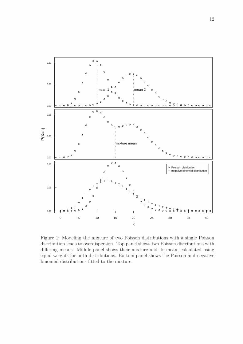
When a single Poisson distribution is used to model the two persons with thesame predictor values, the distribution has a rate parameter that is between the two.However, depicted in Figure 1, the mixture of two Poisson distributions has a largerstandard deviation than a single Poisson distribution with the same mean. There-fore, modeling the mixture with a single Poisson distribution leads to overdispersion.

4.3.3 The negative binomial distribution

The missing predictors in the regression model can be accounted for by adding anerror term to Equation 17,

λ = f(x) + ǫ (25)

y ∼ Poisson(λ), (26)

where ǫ represents the inter-individual variation that cannot be inferred from thepredictors x. Note that the expected value of Poisson distribution is denoted by λ,so E[y] has been replaced by λ in the notation.

A zero-mean normal distribution is a natural choice for the distribution of ǫ,but it yields no closed-form solution for the distribution of y. If ǫ instead follows alog-gamma distribution, the distribution of y can be equivalently written as (proofomitted)

λ = f(x) (27)

y ∼ NB(λ, θ), (28)

where NB denotes the negative binomial distribution.The negative binomial distribution resembles the Poisson distribution, but

it has two parameters instead of one: the rate parameter λ controls the mean of the

12

mean 1 mean 2

0.00

0.06

0.12

P(X

=k)

0.00

0.03

0.06

mixture mean

k

0 5 10 15 20 25 30 35 40

0.00

0.05

0.10Poisson distributionnegative binomial distribution

Figure 1: Modeling the mixture of two Poisson distributions with a single Poissondistribution leads to overdispersion. Top panel shows two Poisson distributions withdiffering means. Middle panel shows their mixture and its mean, calculated usingequal weights for both distributions. Bottom panel shows the Poisson and negativebinomial distributions fitted to the mixture.

13

distribution, and the rate parameter λ and the dispersion parameter together θcontrol the standard deviation,

E[y] = λ (29)

Sd[y] =

√

λ+λ2

θ. (30)

As seen in Equation 30, Sd[y] →√λ as θ → ∞, which reduces the negative binomial

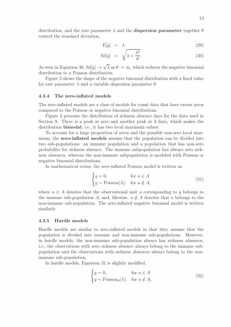
distribution to a Poisson distribution.Figure 2 shows the shape of the negative binomial distribution with a fixed value

for rate parameter λ and a variable dispersion parameter θ.

4.3.4 The zero-inflated models

The zero-inflated models are a class of models for count data that have excess zeroscompared to the Poisson or negative binomial distributions.

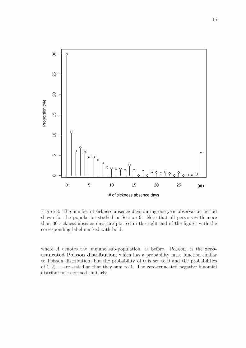
Figure 3 presents the distribution of sickness absence days for the data used inSection 9. There is a peak at zero and another peak at 3 days, which makes thedistribution bimodal, i.e., it has two local maximum values.

To account for a large proportion of zeros and the possible non-zero local max-imum, the zero-inflated models assume that the population can be divided intotwo sub-populations: an immune population and a population that has non-zeroprobability for sickness absence. The immune subpopulation has always zero sick-ness absences, whereas the non-immune subpopulation is modeled with Poisson ornegative binomial distributions.

In mathematical terms, the zero-inflated Poisson model is written as{

y = 0, for u ∈ A

y ∼ Poisson(λ), for u /∈ A,(31)

where u ∈ A denotes that the observational unit u corresponding to y belongs tothe immune sub-population A, and, likewise, u /∈ A denotes that u belongs to thenon-immune sub-population. The zero-inflated negative binomial model is writtensimilarly.

4.3.5 Hurdle models

Hurdle models are similar to zero-inflated models in that they assume that thepopulation is divided into immune and non-immune sub-populations. However,in hurdle models, the non-immune sub-population always has sickness absences,i.e., the observations with zero sickness absence always belong to the immune sub-population and the observations with sickness absences always belong to the non-immune sub-population.

In hurdle models, Equation 31 is slightly modified,{

y = 0, for u ∈ A

y ∼ Poisson0(λ), for u /∈ A,(32)

14

0.00

0.05

0.10

0.15

0.20

0.25

0.30

0.35 λ = 15, θ = 0.25

0.00

0.05

0.10

0.15

0.20

θ = 0.5

P(X

=k)

0.00

0.05

0.10θ = 1

0.00

0.05

0.10θ = 2

k

0.00

0.05

0.10

0 5 10 15 20 25 30

θ = 10

Figure 2: The probability mass function of the negative binomial distribution withfixed rate parameter λ and variable dispersion parameter θ. The shape of the dis-tribution resembles Poisson distribution for large values of θ (bottom-most panel),and as θ decreases, small values obtain more probability mass.

15

05

1015

2025

30

# of sickness absence days

Pro

port

ion

(%)

0 5 10 15 20 25 30+

Figure 3: The number of sickness absence days during one-year observation periodshown for the population studied in Section 9. Note that all persons with morethan 30 sickness absence days are plotted in the right end of the figure, with thecorresponding label marked with bold.

where A denotes the immune sub-population, as before. Poisson0 is the zero-truncated Poisson distribution, which has a probability mass function similarto Poisson distribution, but the probability of 0 is set to 0 and the probabilitiesof 1, 2, . . . are scaled so that they sum to 1. The zero-truncated negative binomialdistribution is formed similarly.

16

4.4 The generalized linear models

So far, we have considered models for the distribution of the response variable,i.e., the stochastic part of the regression model framework of Equations 17 and 18.The deterministic part, or choosing function f in E[y] = f(x), is the other step inspecifying the model.

In Section 3, we introduced the linear model, in which a linear relationship wasassumed between E[y] and x, and y was assumed to be normally distributed. Thegeneralized linear models (McCullagh & Nelder, 1989; not to be confused withthe general linear model) extend linear regression to non-normal distributions of theobservations and to cases where the range of the observations is restricted.

The expected value of a count is always non-negative, so count data serves as anexample of restricted range of the observations. With count data, modeling E[y] asa linear function of x does not work, because a linear function obtains both negativeand positive values.

To account for the restrictions, generalized linear models use a link function,which maps the expected value of the model to the range of the linear function.This is denoted as

g(E[y]) = xTβ (33)

y ∼ Distr(E[y]), (34)

where g is the link function and Distr is an arbitrary distrition, as before.The mean function is the inverse of link function. Written in terms of the

mean function, Equations 33 and 34 become

E[y] = g−1(xTβ) (35)

y ∼ Distr(E[y]), (36)

where g−1 denotes the mean function. For clarity, we use only the mean function inthe models we present.

4.4.1 Linear model

The generalized linear models contain the linear model introduced in Section 3 as aspecial case: With mean function f(x) = x and normally distributed y, the modelin Equations 35 and 36 reduces to the linear model.

4.4.2 Poisson regression model

ThePoisson regression model is an example of a generalized linear model, writtenas

E[y] = exp(xTβ) (37)

y ∼ Poisson(E[y]), (38)

where the exponential mean function ensures that E[y] is positive.

17

4.4.3 Logistic regression model

The logistic regression model is used for classification,

µ = logit−1(xTβ) (39)

y ∼ Bernoulli(µ), (40)

where the mean function is called the logistic function, defined as

logit−1(x) = (1 + exp(x))−1 . (41)

The logistic function maps the range (−∞,∞) to the range (0, 1).The observation y is Bernoulli(p) distributed, i.e., it attains value 1 with prob-

ability p and value 0 with probability 1− p. In classification, value 1 is interpretedas belonging to class A and value 0 as not belonging to class A.

4.4.4 Negative binomial regression model

Similarly, adding a generalized linear part to the negative binomial model in Equa-tions 27 and 28 yields

λ = exp(xTβ) (42)

y ∼ NB(λ, θ). (43)

In the negative binomial model, β and θ are the model parameters. In principle,both θ and λ can depend on the predictors but usually θ is modeled without them.

4.4.5 Zero-inflated and hurdle models

The zero-inflated and hurdle negative binomial models in the generalized linearmodel framework consist of modeling λ, as in Equation 42, and using a logisticregression model for the classification,

{

y = 0, for u ∈ A

y ∼ NB(λ, θ), for u /∈ A,(44)

where P (u ∈ A) = µ, and

λ = exp(xTβm) (45)

µ = logit−1(xTβc). (46)

In hurdle models, the negative binomial distribution NB is replaced by the truncatednegative binomial distribution, denoted by NB0.

Note that two groups of regression coefficients are needed for the zero-inflatedmodel, βm for modeling the mean λ, and βc for classification.

18

5 Regression with Gaussian processes

This Section is based on Rasmussen & Williams (2006) and Vanhatalo et al. (2011),who consider many issues ignored here, e.g., detailed algorithms for computationwith Gaussian process models.

In this Section, we introduce Gaussian process models, which are flexible non-linear regression models. They can be used to find non-linear relationships betweenpredictors and the response variable. Gaussian process models also automaticallyassess interactions between the predictors.

5.1 An introduction to Gaussian process models

In Equation 16, we wrote y as a function f of the predictors x. Unlike generalizedlinear models, Gaussian process models assume a random f so that the values of ffollow a zero-mean Gaussian distribution.

Specifically, at each data point xi,

E[yi] = f(xi) ∼ N(0, σ2

i ). (47)

The function f is called the latent function, as it is not observed directly, butonly through the observations yi. As before, the values of y follow an arbitrarydistribution around their mean.

Similarly to generalized linear models, we can restrict range of E[y] by usinga mean function. For instance, if yi follows a Poisson distribution, an exponentialmean function can be used to ensure that E[y] is non-negative.

Using the short-hand notation fi = f(xi),

E[yi] = g−1(fi) (48)

fi ∼ N(0, σ2

i ), (49)

where g−1 is the mean function. Note that mean function is also used in non-zero-mean Gaussian processes, where it refers to the function that specifies the mean ofthe process. However, in this text, we only consider zero-mean Gaussian processes,avoiding the risk of confusion.

The next step in formulating the Gaussian process model is adding covariancebetween data points. This is done using a covariance function, Cov(fi, fj), whichspecifies the covariance as a function of two latent variables, fi and fj. Covarianceis added because if the distributions of fi for different data points xi were mutuallyindependent, the data (xi, yi), 1 ≤ i ≤ n, do not affect the distribution of f∗ for anew data point x∗, and therefore does not affect predictions for x∗.

When xi and xj are close to each other, it is a reasonable modeling assumptionthat the corresponding values of f covary more than when they are farther apart.This gives rise to a class of covariance functions called the radial basis covariancefunctions, which depend only on the distance between xi and xj, i.e.,

Cov(fi, fj) = φ(||xi − xj||) = φ(r). (50)

19

A commonly used covariance function is the squared exponential function,

Cov(fi, fj) = σ2 exp

[

−( ||xi − xj||

l

)2]

, (51)

where σ2 is the variance of each xi. l is called the length scale, and it specifieshow quickly the covariance decreases when the distance between two data pointsincreases. l and σ2 are the parameters of the covariance function, and for now, weconsider them fixed. Later, we present methods for optimizing them as a part ofthe modeling.

The covariances between pairs of the observed data points xi,xj, 1 ≤ i, j ≤ nform the covariance matrix K. In Gaussian processes, the data points xi reduceto the covariance matrix K, i.e., we do not the data points themselves beyondcomputing K.

Gaussian processes are non-parametric models, so the function f(xi) itself doesnot have parameters. This is in contrast to the generalized linear models, where theinference consists of optimizing the parameters of f . However, if we consider f as arandom vector of n dimensions and a Gaussian distribution specified by K, i.e.,

f ∼ N(0, K). (52)

we can condition the latent values f on the observations y. Informally, this isinterpreted as drawing samples for f and discarding those that disagree with theobservations y. Formally, we do Bayesian inference for f ,

p(f |y) = p(y|f)p(f)p(y)

. (53)

Note that the posterior distribution p(f |y) is not necessarily Gaussian, althoughp(f) is. Also, in contrast to the usual application of the Bayes’ theorem to computethe parameter posterior, here the inference is done for the latent function f . In asense, the latent function values fi at the points xi can be interpreted as the modelparameters, as they and the parameters of the covariance function govern the modelbehaviour.

p(f) is often called a Gaussian process prior for the latent values f , which isconsistent with the above interpretation and Bayesian terminology. The parametersof the covariance function are called the model hyperparameters.

5.2 Prediction with Gaussian processes

Contrary to parametric models, e.g., the linear model, the inferred latent posteriorp(f |y) is usually not of primary interest in Gaussian process models. However, thelatent posterior provides updated knowledge about the latent function f , which canbe used to update knowledge about f at points other than xi, and ultimately makepredictions about y.

20

For prediction, we examine an arbitrary test point, denoted by x∗. The cor-responding latent function value is denoted by f∗. The latent posterior at the testpoint x∗, i.e., p(f∗|y), is calculated by integrating over the latent posterior p(f |y),

p(f∗|y) =∫

p(f∗|f)p(f |y)df . (54)

The uncertainty about f∗ can be further propagated to compute the posteriorpredictive distribution for y∗,

p(y∗|y) =∫

p(y∗|f∗)p(f∗|y)df∗. (55)

The posterior predictive distribution is a distribution for the predictions of y, i.e.,it can be used to draw predictions or compute statistics of interest, for exampleposterior predictive mean.

5.3 The optimization of the hyperparameters

So far, the parameters of the covariance function, i.e., the hyperparameters, havebeen fixed. However, an essential part of Gaussian process modeling is to findreasonable values for the hyperparameters.

If hyperparameters are allowed to vary, the prior p(f) becomes conditional onthe hyperparameters, denoted by p(f |θ), where θ is the hyperparameter vector. Forfull Bayesian inference, a prior p(θ) is also needed for the hyperparameters.

Earlier, we computed the latent posterior p(f |y) with regard to the observationsy. We now do the same for hyperparameters,

p(θ|y) = p(y|θ)p(θ)p(y)

. (56)

p(y|θ) is related to the value of θ only through the latent function f , so it cannotbe calculated directly. Therefore, we compute p(y|θ) by integrating over f :

p(y|θ) =∫

p(y|f)p(f |θ)df . (57)

The hyperparameter posterior p(θ|y) can be used in two ways. First, a point esti-mate for θ can be computed, in which case we maximize p(θ|y) with regard to θ.This yields the maximum a posteriori (MAP) estimate for θ,

θ = argmaxθ

p(θ|y). (58)

Once a value for θ is set, we can proceed with the inference as shown previously.Second, we can take into account the whole hyperparameter posterior p(θ|y)

and propagate the uncertainty in θ to the latent prior p(f |θ) and on to the posteriorpredictive distribution p(y∗|y, θ). This is done by first sampling the hyperparameter

21

posterior p(θ|y), doing the inference individually for each sample, and then com-bining the obtained posterior predictive distributions. For that, the law of totalvariance and the law of total expectation are used,

E[y∗|y] = Eθ[E[y∗|y, θ]] (59)

Var[y∗|y] = Eθ[Var[y∗|y, θ]] + Varθ[E[y∗|y, θ]]. (60)

Using Equations 59 and 60, the expectations and variances of the posterior pre-dictive distribution, p(y∗|y), can be combined for different values of θ to obtain theexpected value and variance of the posterior predictive distribution, to which theuncertainty in θ has been propagated.

5.4 Computation with Gaussian processes

Once the Gaussian process prior p(f) and the likelihood function p(y|f) are selected,the posterior predictive distribution p(y∗|y) can be computed for the test point x∗

by combining Equations 53, 54, and 55. However, the actual computation of p(y∗|y)is often difficult.

In the simplest case, we assume a normal observation model. Using a Gaussianprocess prior p(f) and a normal likelihood p(y|f), the posterior p(f |y) in Equation 53is normally distributed. This results in normally distributed posterior predictivedistribution p(y∗|y), the parameters of which can be analytically solved.

However, if the likelihood is not Gaussian, the latent posterior p(f |y) is notGaussian either, and the integral in 54 becomes analytically intractable. We canstill solve the integral by using Monte Carlo sampling or analytic approximationsto the latent posterior. Monte Carlo sampling will not be considered here, but nextwe present a method for approximating the latent posterior, namely, the Laplaceapproximation.

5.4.1 Laplace approximation

The Laplace approximation is a general method for approximating the posteriordistribution in Bayesian inference. It approximates the posterior by a normal distri-bution, which is a good approximation because the posterior often resembles the nor-mal distribution. The normal distribution is also analytically well-behaved, whichmakes the approximation particularly useful.

The normal distribution in multiple dimensions, called the multivariate nor-mal distribution, has two parameters, the mean and the covariance matrix InLaplace approximation, the values of the parameters are obtained from the second-order Taylor polynomial of the logarithm of the approximating distribution aroundits mode,

log(p(x)) ≈ log(p(x)) +∇ log(p(x)(x− x) +1

2(x− x)T∇∇ log(p(x))(x− x), (61)

where p(x) is the approximated distribution, x is the mode of p(x), and ∇∇ denotesthe Hessian.

22

By definition, ∇ log(p(x)) = 0 at the mode of log(p(x)), so Equation 61 reducesto

log(p(x)) ≈ log(p(x)) +1

2(x− x)T∇∇ log(p(x))(x− x). (62)

From that, we obtain an approximation for p(x) by exponentiating,

p(x) ≈ p(x) exp

(

1

2(x− x)T∇∇ log(p(x))(x− x)

)

. (63)

The right-hand side of Equation 63 is identified as the unnormalised multivariatenormal distribution with the mean x and the covariance matrix Σ = −∇∇ log(p(x)).

Although there are posterior approximations better than the Laplace approxi-mation, namely, expectation propagation (Minka, 2001), we use Laplace approxi-mation in modeling sickness absence in Section 9 because it was found more stablewith complex Gaussian process models.

5.5 The connection between Gaussian process models andgeneralized linear models

Using a Gaussian process model with the linear covariance function, laitakaava!,reduces the model to the generalized linear model. We present this result withoutjustification, but an interested reader is recommended to turn to Rasmussen &Williams (2006) for a discussion of the weight space view and the function spaceview of Gaussian processes.

We use this result in Section 9 for comparing Gaussian process models to gen-eralized linear models directly, using the same toolbox and the same algorithms formodeling.

5.6 Specifying the Gaussian process model

AGaussian process model is specified by setting the functional form of the covariancefunction and specifying the relationship between the response variable y and thelatent function f .

Analogously to the generalized linear models, the Gaussian process model iswritten as

f ∼ GP (0,Cov(x,x′)) (64)

y ∼ Distr(g(f)). (65)

Equation 64 specifies that the latent function f is a zero-mean Gaussian processwith the covariance function Cov(x,x′), and Equation 65 links the latent value f tothe mean of the distribution Distr by the mean function g.

We use the Poisson model, negative binomial model, and hurdle negative bino-mial model in the comparison of Gaussian process models in Section 9, so they arepresented in detail next.

23

5.6.1 Poisson and negative binomial Gaussian process models

The Poisson Gaussian process model is written as

f ∼ GP (0,Cov(x,x′)) (66)

y ∼ z · Poisson(exp(f)). (67)

The coefficient z is used to match the Poisson distribution to the average values ofy because the latent function f is zero-mean.

The coefficient z is often calculated as the average over the observations, but itcan also be specified pointwise, e.g., in spatial epidemiology when considering areasof different sizes.

The negative binomial Gaussian process model is written similarly as

f ∼ GP (0,Cov(x,x′)) (68)

y ∼ z · NB(exp(f), θ). (69)

and a logistic Gaussian process model for classification as

f ∼ GP (0,Cov(x,x′)) (70)

y ∼ logit−1(exp(f)). (71)

5.6.2 Zero-inflated and hurdle Gaussian process models

The zero-inflated Poisson and negative binomial models are written in the Gaussianprocess framework as

f1 ∼ GP (0,Cov(x,x′|θ1)) (72)

f2 ∼ GP (0,Cov(x,x′|θ2)) (73)

µ = logit−1(f1) (74)

λ = exp(f2), (75)

where µ is the probability that the observation belongs to the immune sub-populationand λ is the expected number of sickness absence days if the observation belongs tothe non-immune sub-population.

As seen in Equations 72 and 73, the zero-inflated Gaussian process models usetwo latent functions, one for the zero part and one for count part. Zeros in the datacan be generated by either part, so the likelihood of zero depends on both parts,which makes the modeling more difficult than with either part alone.

In hurdle models, zeros and non-zeros can only be generated by the zero partand the count part, respectively, which makes hurdle models simpler to implementwith Gaussian processes. For a zero observation, we use the latent function f1,

f1 ∼ GP (0,Cov(x,x′|θ1)) (76)

µ = logit−1(f1) (77)

p(y) = µ, (78)

24

and for non-zero observation, we use f2,

f2 ∼ GP (0,Cov(x,x′|θ2)) (79)

λ = exp(f2) (80)

y ∼ NB0(µ). (81)

That is, the two parts can be modeled independently from each other.

5.7 Advantages of using Gaussian process regression

There are several advantages in using Gaussian process regression compared to thegeneralized linear models. These can be summarized by considering the type ofrelationships that can be modeled with each.

In generalized linear models, as described in Section 4, the relationship betweeneach predictor and the response variable is linear, apart from the mean function,which introduces nonlinearity to the relationship. However, the mean function isusually monotonic, i.e., it either increases or decreases. Therefore, the relationshipas a whole is monotonic.

With Gaussian processes, the predictor and the response variable may depend oneach other non-linearly. The difference between a linear and a non-linear relationshipis depicted with simulated data in Figure[??]. As seen, the generalized linear modeldoes not detect the nonlinearity present in the relationship.

In practice, nonlinear relationships arise often. For instance, instead of a low orhigh value, an average predictor value might minimize or maximize the response.When studying factors associated with sickness absence or health in general, e.g.,the body-mass index is a good candidate for such predictor.

5.8 The presentation of results

In contrast to the generalized linear models, which can be summarized using regres-sion coefficients, the primary output of Gaussian process regression is the posteriorpredictive distribution of the response variable at a test point x∗. Therefore, theGaussian process regression has to be summarized in another way.

One summary can be obtained by considering what happens to the responsevariable when one of the predictors changes while the others remain fixed at theiraverage values. This is done by computing the posterior predictive distributions atthe corresponding test points, and summarizing them, e.g., by calculating mean.

Another summary, namely, average predictive comparisons, presented in Chap-ter 7, is based on evaluating the average change in the response variable for theaverage change of the predictor. Average predictive comparisons can be used alsofor Gaussian processes, but non-linear relationships are not explicitly seen in it.

25

6 Model selection

In this Section, we present two methods for selecting between different regressionmodels, namely, Akaike information criterion (AIC) and cross-validation. The meth-ods are not specific to regression models, so they are presented in their general form.

6.1 Akaike information criterion

The Akaike information criterion (AIC, see, e.g., Bishop, 2006) is a model selectioncriterion based on information theory. AIC is a fundamentally a frequentist criterion,for example, it does not take into account prior knowledge. However, it is commonlyused to compare generalized linear models, which is why we use it as reference formodel selection.

AIC is defined asAIC = 2k − 2 ln(L), (82)

where k is the number of model parameters and L is the likelihood of the data withthe current model and its parameters.

The lower the AIC, the better the model is. As seen in Equation 82, if the likeli-hood does not change, increasing the number of parameters deteriorates the model,whereas increasing likelihood while the number of parameters is fixed improves themodel.

The number of model parameters is a measure of the model complexity, so thefirst term in Equation 82 can be interpreted as a penalty term for too complexmodels.

6.2 Holdout validation

Before cross-validation, we present a simpler variant, called holdout validation.In holdout validation, a part of the data, called the training dataset, is used toinfer the model, and the rest of the data, the test dataset, is used to evaluate themodel. The test dataset is not used in training the model, so it can be interpretedas unseen or future data. Therefore, the model performance on the test datasetmeasures the predictive performance of the model.

6.3 Cross-validation

In cross-validation, a part of the data is repeatedly held out to be used as the testdataset, until all data are tested once. The test datasets are usually non-overlapping,i.e., each data point is used exactly once for testing the model.

The predictive performance of the model is then combined over the test datasets,e.g., by mean of the performance criterion.

If the number of repetitions in cross-validation is a constant k, it is called k-fold cross-validation. The special case where the number of repetitions equalsthe number of observations is called leave-one-out cross-validation.

26

6.4 Cross-validation using log predictive densities

Evaluating the model on the test dataset requires a measure of performance. Incross-validation, the actual observations at the test datapoints are known, so theperformance measure can compare the model predictions to the observations.

In Bayesian analysis, the model yields predictive distributions instead of pointpredictions. The predictive distributions can be assessed with an utility function(Vehtari & Lampinen, 2002).

An utility function is defined such that its parameters are a predictive distribu-tion and an observation, and the function returns a value that reflects the discrep-ancy between the distribution and the observation. An example of a discrepancymeasure is the negative mean squared error (MSE) between the observation and theexpected value of the distribution. This can be written as

U(p(x), xobs) = − |E[p(x)]− xobs|2 . (83)

Often, the negative MSE is not a good utility function, as it compares the ob-servation only to the expected value of the distribution, ignoring most of the infor-mation of the distribution. For instance, two very differently shaped distributionswith equal means always yield the same MSE.

Another choice for the utility function is the logarithm of the predictive densityof the observation (LPD), defined as

U(p(x), xobs) = log (p(xobs)) . (84)

In the case of many observations, we average the utility function over the ob-servations. This yields an overall estimate for the predictive performance of themodel.

In studying sickness absence in Section 9, we use the LPD averaged over theobservations, which is called the mean log predictive density (MLPD), togetherwith leave-one-out cross-validation.

6.5 Comparing cross-validated models using Bayesian boot-

strap

6.5.1 Bootstrap and Bayesian bootstrap

Bootstrap (Efron, 1979) is a non-parametric statistical procedure for estimatingsampling distributions, i.e., the distribution of an estimator over repeated samplingof the population. It is often used when minimal distribution assumptions are pre-ferred or when computing standard errors for estimators for which theoretical resultsof the sampling distribution are not available, e.g., sample standard deviation.

Bootstrap is based on generating additional samples, called bootstrap samples,by sampling the observed data with replacement. This is thought to approximatesampling the population. The samples are then treated as if they were independentsamples from the population.

27

In Bayesian bootstrap (Rubin, 1981), the observed data is sampled with non-uniform distribution, i.e., the probability that an observation is picked for the sampleis not 1/n. Instead, the probabilities are assigned by drawing n − 1 independentrandom numbers uniformly from the interval [0, 1], ordering them, and calculatingthe gaps between successive numbers. For the smallest and the largest number, gapsto 0 and 1, respectively, are calculated. The n gaps are then used as the probabilitiesfor the n observations.

Bayesian bootstrap allows the interpretation of the bootstrap samples as samplesgenerated by draws from the posterior of the estimated statistic, whereas ordinarybootstrap has no such Bayesian interpretation.

6.5.2 Comparing models using Bayesian bootstrap

Cross-validation yields an estimate of the predictive performance of the model ateach test datapoint. Pairwise comparison of the predictions of two models can thenbe done using, e.g., a paired t-test. However, Bayesian bootstrap yields samplesfrom the posterior of the paired difference, which allow a wider range of tests, e.g.,based on correctly inferring the sign of the difference. Also, Bayesian bootstrap is anon-parametric method, so it does not depend on distribution assumptions.

To keep with the Bayesian paradigm, we use Bayesian bootstrap to comparecross-validated models in Section 9.

28

7 Summarizing regression analysis

Commonly, a summary of a regression analysis consists of the credible intervals ofthe regression coefficients (confidence intervals in the case of a frequentist analysis)and a corresponding point estimate, e.g., the posterior mean.

Here, we present another scheme for summarizing the results, average predictivecomparisons (Gelman & Pardoe, 2007). We also present a method for variableselection, based on the probability of knowing the sign of the effect of a predictor(Gelman & Tuerlinckx, 2000).

7.1 Average predictive comparisons

In a linear regression model, the regression coefficients can be interpreted as theaverage change in the response variable when the predictor changes by one. How-ever, in a regression model with nonlinearities, e.g., Gaussian process regression,the change depends on the original predictor value, as well as the values of otherpredictors.

We may still summarize the change in the response variable, assuming a certaininitial combination of the predictor values. For this, the predictive comparisonis defined as

δ(u1 → u2, v, θ) =E[y|u2, v, θ]−E[y|u1, v, θ]

u2 − u1

, (85)

where u1 is the initial value of the predictor of interest, u2 is the changed value, andv consists of all other predictors. θ are the parameters of the model.

The predictive comparison can be interpreted as the expected change in theresponse variable per unit change in the predictor of interest, when the predictor ofinterest changes from u1 to u2 and all other predictors are held constant.

We are interested in computing the average change in the response variable overall increasing transitions u1 → u2 and over every v, weighted by the probability ofeach combination of predictors occurring in the data. This can be estimated by

∆ =

∑n

i=1

∑n

j=1wij (E[y|uj, vi, θ]− E[y|ui, vi, θ]) sign(uj − ui)

∑n

i=1

∑n

j=1wij(u2 − u1) sign(uj − ui)

, (86)

where the sums are taken over all observations, and the weights wij reflect theprobability that uj is observed together with vi. The sign function ensures that onlyincreasing transitions are considered. Equation 86 is called the average predictivecomparison, calculated for the predictor of interest u.

The weights are needed because, in contrast to the predictor combinations ui, viand uj, vj , the probability of observing ui, vj cannot be calculated directly. Instead,the weights can be estimated using Mahalanobis distance,

wij =1

1 + (vi − vj)TΣ−1v (vi − vj)

, (87)

where Σv is the covariance matrix of the components of v.

29

Credible intervals or other statistics of interest for the average predictive com-parisons can be calculated by propagating the uncertainty from the parameters θto the average predictive comparison ∆ in Equation 86. This is typically done bysampling the posterior of θ and calculating the average predictive comparison foreach sample, which samples the posterior of the average predictive comparison.

Both Gaussian process regression and generalized linear models are used in study-ing sickness absence in Section 9, so we summarize the results with average predictivecomparisons.

7.2 Variable selection

Traditionally, predictors in regression are considered relevant based on whether thesign of the regression coefficient reliably differs from zero, which is formalised usingnull hypotheses and p-values.

Gelman and Tuerlinckx (2000) argue that in social sciences, the regression coeffi-cients in principle always differ from zero, which makes the comparison meaningless.Instead, they propose an alternative method, called the Bayesian multiple com-parisons, based on whether the sign of the regression coefficient can be reliablyinferred.

Specifically, they suggest that those variables are considered relevant for whichthe joint posterior probability of correctly inferring the sign of the effect exceedsa pre-specified threshold, e.g., 95%. These variables can be found using a stepwiseprocedure, in which the variable that least decreases the probability is added at eachstep until the probability becomes less than the threshold.

In studying sickness absence in Section 9, we compare Bayesian multiple compar-isons to the traditional method that selects the predictors whose marginal credibleintervals (which are analogous to confidence intervals in non-Bayesian analysis) ex-cludes zero.

7.3 Disadvantages of using complex models

Using a more complex model is not always preferable, even if it has a higher predic-tive performance. The increase in performance can be marginal, albeit statisticallysignificant, and a complex model is more difficult to present and interpret.

For example, zero-inflated models yield two sets of regression coefficients. Theinterpretation of the coefficients is confounded by the model assumptions: Thezero part describes the probability that the individual belongs to the immune sub-population, but the immune sub-population itself is a modeling assumption, so it ispossible that the coefficients of both parts describe the same phenomenon.

For these considerations, we also present the results for a relatively simple model,namely, the negative binomial model, in studying sickness absences in Section 9.

30

8 Considerations for pre-processing the data

8.1 Recoding

To treat different predictors in a consistent manner, we code them as numericalvariables. In some environments, e.g., in R, explicit recoding of non-numerical vari-ables is not necessary for regression analysis, but it might still be helpful for otherpre-processing steps, e.g., imputation, which is considered in Subsection 8.2.

In general, there are two types of non-numerical variables. A categorical variablehas a discrete set of levels that the variable can attain. The levels are not ordered,so, for instance, nationality can be coded as a categorical variable.

In categorical variables, each level has its own indicator variable, i.e., a variablethat is is given the value 1 if the original variable is at the indicated level, and 0otherwise.

In a linear model with a constant term, one of the levels is chosen as the “base-line”, which is coded with each indicator at 0. Otherwise, the constant term willbe linearly dependent on the combination of the indicators, which causes the modelinference to fail.

For example, a variable with the levels “yes”, “no”, “maybe” can be coded as

“yes′′ → (1, 0)

“no′′ → (0, 1)

“maybe′′ → (0, 0).

An ordinal variable also has discrete levels, but the levels are ordered. The ordercan be inherent to the scale, as in Likert scale (“Strongly disagree”, . . ., “Stronglyagree”), or it can be an interpretation of the levels (e.g., the above levels “yes”,“maybe”, and “no”).

Typically, an ordinal variable is coded with consecutive natural numbers suchthat the order is retained, e.g., “yes′′ → 2, “maybe′′ → 1, “no′′ → 0. However, it ispossible to use any monotonically increasing function of the ordered category labels,e.g., to reflect the gap sizes between adjacent categories.

8.2 Handling missing data

Missing data is a problem in most data analysis done on surveys or questionnaires.Imputation, i.e., replacing missing values with their statistical estimates, is com-

monly used for handling missing data. Many authors advocate using multiple im-putation, that is, generating several imputed datasets and combining the estimatesof interest, e.g., regression coefficients.

However, if the rate of missing data is small, as in the study presented in Sec-tion 9, satisfactory results can be obtained using single imputation, i.e., doing theanalysis with only one imputed dataset.

31

8.2.1 Gaussian expectation-maximization algorithm

A general method for both single and multiple imputation is to fit a probabilitydistribution to the observed data and using the distribution to draw samples for themissing values.

To fit the distribution, the expectation-maximization (EM) algorithm canbe used (e.g., Bishop 2007). EM algorithm begins with an initial value for thedistribution parameters and consists of iterating two steps,

1. The expectation step calculates the expected values of the missing data us-ing the current estimate for the probability distribution.

2. The maximization step adjusts the parameters of the distribution to max-imize the likelihood of the current data, which includes the missing valueestimates calculated in the expectation step.

The steps are repeated until the algorithm converges, i.e., the changes in the pa-rameters become small enough.

Using a multivariate normal distribution for fitting yields theGaussian expectation-maximization algorithm.

8.3 Standardizing the data

Standardization (or normalization) refers to transforming several variables to a com-mon scale. In regression analysis, standardization of numerical predictors is a com-mon pre-processing step. This has the effect of making the model parameters com-parable to each other.

Standardization is often done by subtracting the mean and dividing each variableby its standard deviation (sd). This way, the standardized regression coefficientsin a linear model are interpreted as the average change in the response variablecorresponding to a change of 1 sd in the original scale.

This procedure has a drawback. The regression coefficients of discrete predictors,e.g., gender, become non-interpretable as such, as there is no “1 sd change in gen-der.” Various modifications to the standardization procedure have been proposedto overcome this.

The simplest modification is to standardize only non-binary predictors. Thisgives two distinct groups of regression coefficients, which are comparable within butnot between the groups. In this way, the binary predictors, coded with 0–1, retainthe property that the regression coefficient is the average change in the responsevariable as the predictor value changes from 0 to 1.

Gelman has proposed that in addition to not standardizing the binary predictors,the non-binary predictors are standardized by dividing them by 2 sd’s instead of 1sd, yielding them a sd of 0.5. This reduces the gap between the two predictorgroups, because a binary predictor whose both categories are equally likely has a sdof

√

p(1− p) =√0.5 · 0.5 = 0.5. After that, the closer the distribution of the two

32

categories of a binary predictor is to uniform, the more comparable the correspondingregression coefficient is to the regression coefficients of non-binary predictors.

Table 1: A summary of standardization procedures.

Procedure Effect on regression coefficients

Subtract mean. Divideeach predictor by 1 sd.

Coefficients describe the effect of 1 sd changein the predictor and are comparable to eachother; coefficients for binary predictors arenon-interpretable.

Subtract mean. Di-vide each predictor by2 sd’s.

Coefficients describe the effect of 2 sd changein the predictor and are comparable to eachother; coefficients for uniformly distributedbinary predictors describe the difference be-tween the two categories.

Subtract mean. Di-vide each non-binarypredictor by 1 sd.

Coefficients for binary and non-binary pre-dictors are comparable to each other withinbut not between groups; coefficients for binarypredictors remain interpretable.

Subtract mean. Di-vide each non-binarypredictor by 2 sd.

Coefficients for binary and non-binary predic-tors arecomparable to each other within butnot always between groups; coefficients for bi-nary predictors remain interpretable; coeffi-cients for uniformly distributed binary pre-dictors are comparable to coefficients of non-binary predictors.

33

9 Case study: modeling sickness absence with

healthcare questionnaire data

In this Section, we use regression analysis to study factors associated with sicknessabsence. For that, we have data consisting of health questionnaire answers obtainedfrom employees of a Finnish company (n=541) and the corresponding sickness ab-sence days during the one year period before filling the questionnaire.

First, we review previous research on factors associated with sickness absence.Then, we describe current data in detail. After that, we present the regressionmodels used and finally the results.

9.1 Previous research on factors associated with sicknessabsence

Of demographic factors, gender has been strongly associated with sickness absence(females have a higher rate of sickness absence, see, e.g., Kivimaki et al., 2001,Laaksonen et al., 2008). High level of education has also been associated withdecreased sickness absence (Ala-Mursula et al., 2002, Niedhammer et al., 1998). Forage, Duijts et al. (2007) did not find an association to sickness absence in theirmeta-analysis.

Of factors related to physical health, self-rated poor health, diagnosed chronicillnesses (Kivimaki et al., 2001), smoking (e.g., Niedhammer et al., 1998), and highbody-mass index (Ala-Mursula et al., 2002) have been associated with increasedsickness absence.

For alcohol use, Niedhammer et al. (1998) found that abstainers have higher rateof sickness absence, whereas Ala-Mursula et al. (2002) did not find association andKivimaki et al. (2001) found a similar association in one of the two occupationalgroups studied. Vahtera et al. (2002) have proposed a U-shaped relationship be-tween alcohol intake and sickness absence, i.e., moderate consumption is associatedwith lower rate of sickness absence than high or low consumption.

Mental health has also been associated with sickness absence. Psychiatric mor-bidity has been associated especially with long spells of sickness absence (Kivimakiet al., 2001). According to the meta-analysis of Duijts et al. (2007), psychologicalsymptoms and psychosomatic complaints in general are associated with increasedsickness absence.

Also, psychosocial factors at work, e.g., lack of social support (Niedhammer etal., 1998) and bullying (Kivimaki et al., 2000), have been associated with increasedsickness absence.

Taimela et al. (2007) used models similar to our study and found that havingtwo or more health problems in domains of pain, depression, or insomnia is a strongpredictor for sickness absence.

Interactions between gender and other predictors have been found. For example,feeling overloaded at work has been associated with increased sickness absence inmales but not in females (Kivimaki et al., 2000).

34

Also, predictors that were not used in the current study have been found rele-vant for sickness absence, e.g., being unmarried has been strongly associated withincreased sickness absence especially in males (Niedhammer et al., 1998, Kivimakiet al., 2001).

9.2 Data characteristics

The questionnaire contained validated items about, e.g., physical activity, work-related stress, depression, and pain. It was administered as a part of the employees’occupational healthcare.

The response variable consisted of the total number of sickness absence daysduring the one-year period before the administration of the questionnaire–from thebeginning of September in 2008 to the end of August in 2009–gathered from theemployer’s registry.

Previously, sickness absence has been studied using generalized linear models,e.g., in Taimela et al., 2007. We follow the same approach, but in addition, we trya novel method, namely, the Gaussian process regression, introduced in Section 5.

The present study belongs to a larger study (Reijonsaari et al., 2009), whichinvestigates the effects of a physical activity intervention on a large group of em-ployees. Therefore, the study population consisted of only those employees who werewilling to participate in the one-year-long intervention study and were not excluded.

The exclusion criteria for the intervention study consisted of medical reasons,e.g., pregnancy or disorders that make physical activity dangerous. The completelist and a detailed description of the questionnaire items is found in Reijonsaari etal., 2009.

9.3 Data pre-processing

One participant did not return the questionnaire, and two participants denied the useof their sickness absence data. After these removals, the study population consistedof 541 employees.

The missing data in the questionnaire was imputed using the expectation-maximization(EM) algorithm with a multivariate Gaussian distribution. The imputation was doneusing pmtk3 (Murphy & Dunham, 2008) package in MATLAB. The missing datarate was low (1.1%), so single imputation was used.

There were in total 106 questionnaire items. Of these, 24 items were pre-selectedwith expert help, considering them potentially related to sickness absence. The itemswere then divided into four groups, which consisted of items related to different areasof life. The items and the corresponding groups are listed in Table 2,

We transformed the sickness absence days to make them comparable betweensubjects. First, we calculated the potential working days for each subject, in whichmaternal leaves and other non-sickness related absences were excluded. Then, wescaled the sickness absence days for each subject by the ratio of their potential work-ing days and the maximum number of potential working days in a year, typically 220

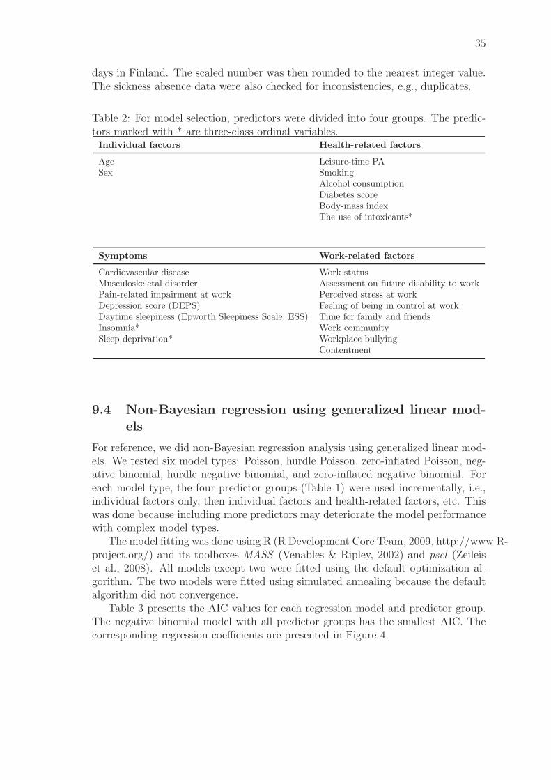
35

days in Finland. The scaled number was then rounded to the nearest integer value.The sickness absence data were also checked for inconsistencies, e.g., duplicates.

Table 2: For model selection, predictors were divided into four groups. The predic-tors marked with * are three-class ordinal variables.Individual factors Health-related factors

Age Leisure-time PASex Smoking

Alcohol consumptionDiabetes scoreBody-mass indexThe use of intoxicants*

Symptoms Work-related factors

Cardiovascular disease Work statusMusculoskeletal disorder Assessment on future disability to workPain-related impairment at work Perceived stress at workDepression score (DEPS) Feeling of being in control at workDaytime sleepiness (Epworth Sleepiness Scale, ESS) Time for family and friendsInsomnia* Work communitySleep deprivation* Workplace bullying

Contentment

9.4 Non-Bayesian regression using generalized linear mod-

els

For reference, we did non-Bayesian regression analysis using generalized linear mod-els. We tested six model types: Poisson, hurdle Poisson, zero-inflated Poisson, neg-ative binomial, hurdle negative binomial, and zero-inflated negative binomial. Foreach model type, the four predictor groups (Table 1) were used incrementally, i.e.,individual factors only, then individual factors and health-related factors, etc. Thiswas done because including more predictors may deteriorate the model performancewith complex model types.

The model fitting was done using R (R Development Core Team, 2009, http://www.R-project.org/) and its toolboxes MASS (Venables & Ripley, 2002) and pscl (Zeileiset al., 2008). All models except two were fitted using the default optimization al-gorithm. The two models were fitted using simulated annealing because the defaultalgorithm did not convergence.

Table 3 presents the AIC values for each regression model and predictor group.The negative binomial model with all predictor groups has the smallest AIC. Thecorresponding regression coefficients are presented in Figure 4.

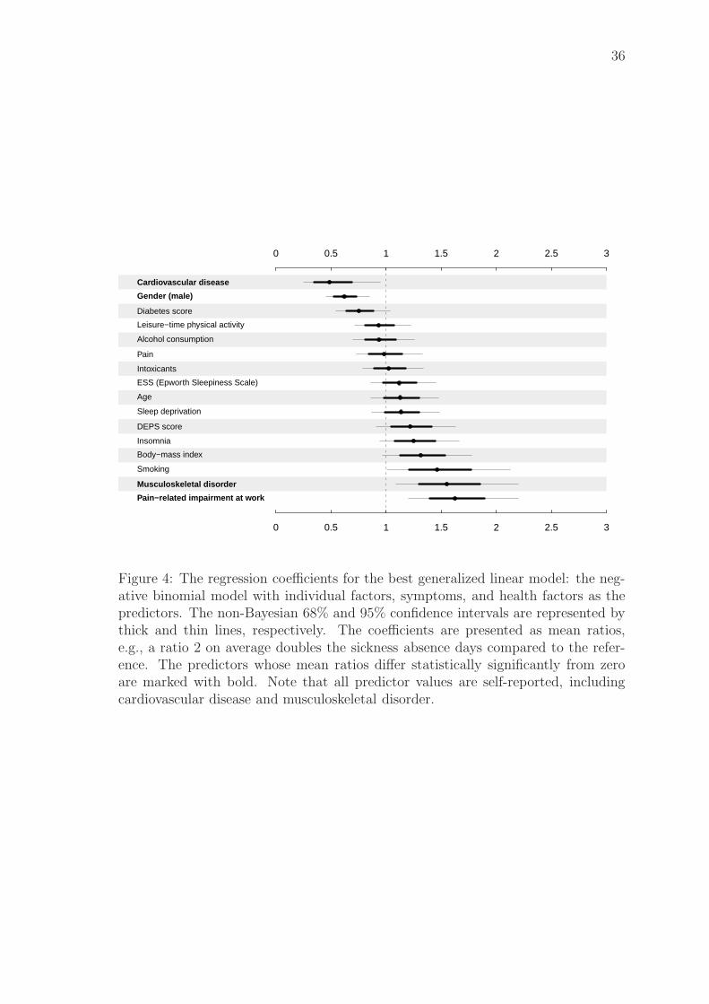
36

Cardiovascular disease

Gender (male)

Diabetes score

Leisure−time physical activity

Alcohol consumption

Pain

Intoxicants

ESS (Epworth Sleepiness Scale)

Age

Sleep deprivation

DEPS score

Insomnia

Body−mass index

Smoking

Musculoskeletal disorder

Pain−related impairment at work

0

0

0.5

0.5

1

1

1.5

1.5

2

2

2.5

2.5

3

3

Figure 4: The regression coefficients for the best generalized linear model: the neg-ative binomial model with individual factors, symptoms, and health factors as thepredictors. The non-Bayesian 68% and 95% confidence intervals are represented bythick and thin lines, respectively. The coefficients are presented as mean ratios,e.g., a ratio 2 on average doubles the sickness absence days compared to the refer-ence. The predictors whose mean ratios differ statistically significantly from zeroare marked with bold. Note that all predictor values are self-reported, includingcardiovascular disease and musculoskeletal disorder.

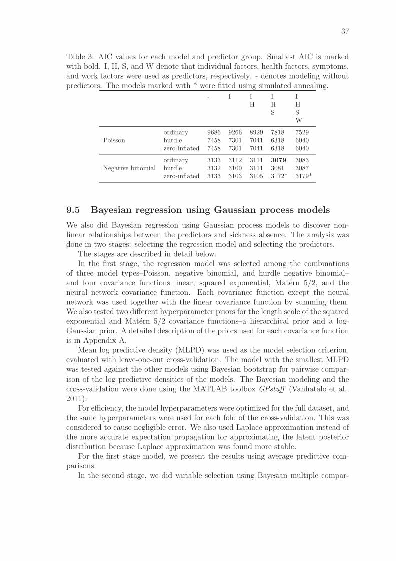
37

Table 3: AIC values for each model and predictor group. Smallest AIC is markedwith bold. I, H, S, and W denote that individual factors, health factors, symptoms,and work factors were used as predictors, respectively. - denotes modeling withoutpredictors. The models marked with * were fitted using simulated annealing.

- I I I IH H H

S SW

Poissonordinary 9686 9266 8929 7818 7529hurdle 7458 7301 7041 6318 6040zero-inflated 7458 7301 7041 6318 6040

Negative binomialordinary 3133 3112 3111 3079 3083hurdle 3132 3100 3111 3081 3087zero-inflated 3133 3103 3105 3172* 3179*

9.5 Bayesian regression using Gaussian process models

We also did Bayesian regression using Gaussian process models to discover non-linear relationships between the predictors and sickness absence. The analysis wasdone in two stages: selecting the regression model and selecting the predictors.

The stages are described in detail below.In the first stage, the regression model was selected among the combinations

of three model types–Poisson, negative binomial, and hurdle negative binomial–and four covariance functions–linear, squared exponential, Matern 5/2, and theneural network covariance function. Each covariance function except the neuralnetwork was used together with the linear covariance function by summing them.We also tested two different hyperparameter priors for the length scale of the squaredexponential and Matern 5/2 covariance functions–a hierarchical prior and a log-Gaussian prior. A detailed description of the priors used for each covariance functionis in Appendix A.

Mean log predictive density (MLPD) was used as the model selection criterion,evaluated with leave-one-out cross-validation. The model with the smallest MLPDwas tested against the other models using Bayesian bootstrap for pairwise compar-ison of the log predictive densities of the models. The Bayesian modeling and thecross-validation were done using the MATLAB toolbox GPstuff (Vanhatalo et al.,2011).

For efficiency, the model hyperparameters were optimized for the full dataset, andthe same hyperparameters were used for each fold of the cross-validation. This wasconsidered to cause negligible error. We also used Laplace approximation instead ofthe more accurate expectation propagation for approximating the latent posteriordistribution because Laplace approximation was found more stable.

For the first stage model, we present the results using average predictive com-parisons.

In the second stage, we did variable selection using Bayesian multiple compar-

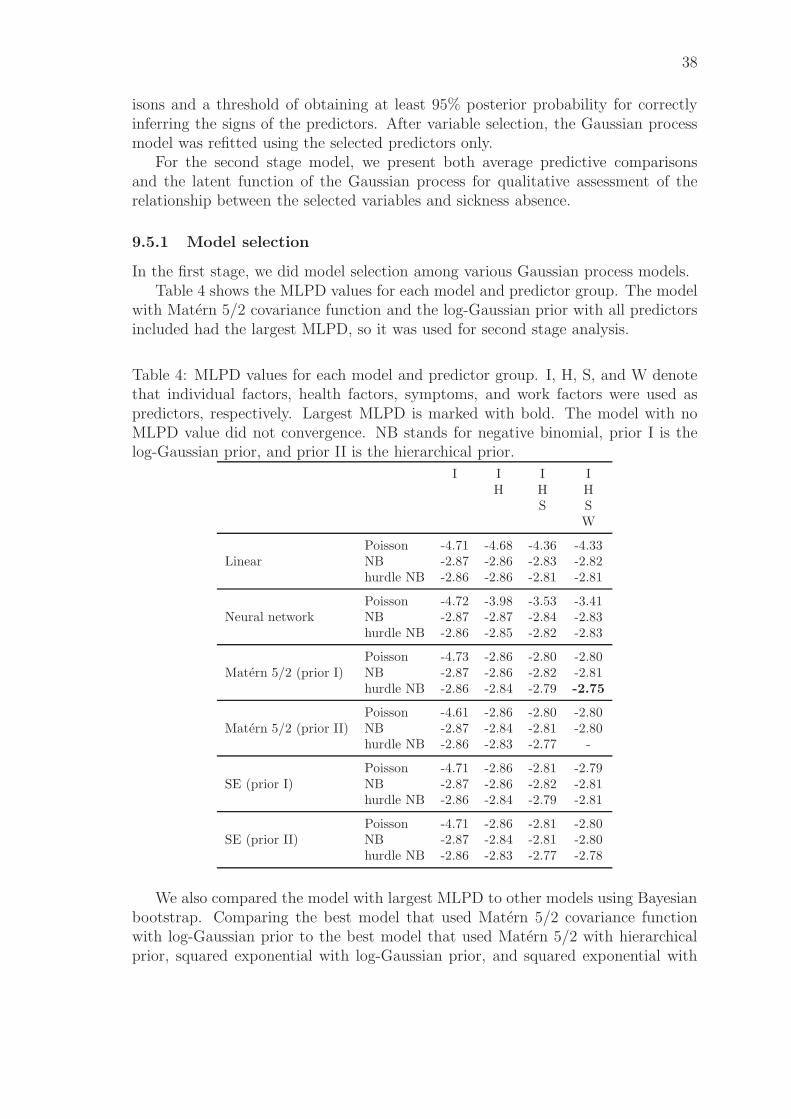
38

isons and a threshold of obtaining at least 95% posterior probability for correctlyinferring the signs of the predictors. After variable selection, the Gaussian processmodel was refitted using the selected predictors only.

For the second stage model, we present both average predictive comparisonsand the latent function of the Gaussian process for qualitative assessment of therelationship between the selected variables and sickness absence.

9.5.1 Model selection

In the first stage, we did model selection among various Gaussian process models.Table 4 shows the MLPD values for each model and predictor group. The model

with Matern 5/2 covariance function and the log-Gaussian prior with all predictorsincluded had the largest MLPD, so it was used for second stage analysis.

Table 4: MLPD values for each model and predictor group. I, H, S, and W denotethat individual factors, health factors, symptoms, and work factors were used aspredictors, respectively. Largest MLPD is marked with bold. The model with noMLPD value did not convergence. NB stands for negative binomial, prior I is thelog-Gaussian prior, and prior II is the hierarchical prior.

I I I IH H H

S SW

LinearPoisson -4.71 -4.68 -4.36 -4.33NB -2.87 -2.86 -2.83 -2.82hurdle NB -2.86 -2.86 -2.81 -2.81

Neural networkPoisson -4.72 -3.98 -3.53 -3.41NB -2.87 -2.87 -2.84 -2.83hurdle NB -2.86 -2.85 -2.82 -2.83

Matern 5/2 (prior I)Poisson -4.73 -2.86 -2.80 -2.80NB -2.87 -2.86 -2.82 -2.81hurdle NB -2.86 -2.84 -2.79 -2.75

Matern 5/2 (prior II)Poisson -4.61 -2.86 -2.80 -2.80NB -2.87 -2.84 -2.81 -2.80hurdle NB -2.86 -2.83 -2.77 -

SE (prior I)Poisson -4.71 -2.86 -2.81 -2.79NB -2.87 -2.86 -2.82 -2.81hurdle NB -2.86 -2.84 -2.79 -2.81

SE (prior II)Poisson -4.71 -2.86 -2.81 -2.80NB -2.87 -2.84 -2.81 -2.80hurdle NB -2.86 -2.83 -2.77 -2.78

We also compared the model with largest MLPD to other models using Bayesianbootstrap. Comparing the best model that used Matern 5/2 covariance functionwith log-Gaussian prior to the best model that used Matern 5/2 with hierarchicalprior, squared exponential with log-Gaussian prior, and squared exponential with

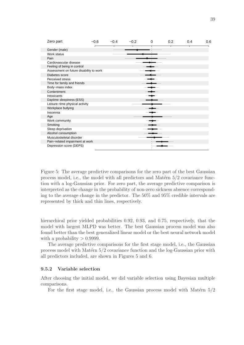
39

Gender (male)Work statusPainCardiovascular diseaseFeeling of being in controlAssessment on future disability to workDiabetes scorePerceived stressTime for family and friendsBody−mass indexContentmentIntoxicantsDaytime sleepiness (ESS)Leisure−time physical activityWorkplace bullyingInsomniaAgeWork communitySmokingSleep deprivationAlcohol consumptionMusculoskeletal disorderPain−related impairment at workDepression score (DEPS)

Zero part −0.6 −0.4 −0.2 0 0.2 0.4 0.6

Figure 5: The average predictive comparisons for the zero part of the best Gaussianprocess model, i.e., the model with all predictors and Matern 5/2 covariance func-tion with a log-Gaussian prior. For zero part, the average predictive comparison isinterpreted as the change in the probability of non-zero sickness absence correspond-ing to the average change in the predictor. The 50% and 95% credible intervals arerepresented by thick and thin lines, respectively.

hierarchical prior yielded probabilities 0.92, 0.93, and 0.75, respectively, that themodel with largest MLPD was better. The best Gaussian process model was alsofound better than the best generalized linear model or the best neural network modelwith a probability > 0.9999.

The average predictive comparisons for the first stage model, i.e., the Gaussianprocess model with Matern 5/2 covariance function and the log-Gaussian prior withall predictors included, are shown in Figures 5 and 6.

9.5.2 Variable selection

After choosing the initial model, we did variable selection using Bayesian multiplecomparisons.

For the first stage model, i.e., the Gaussian process model with Matern 5/2

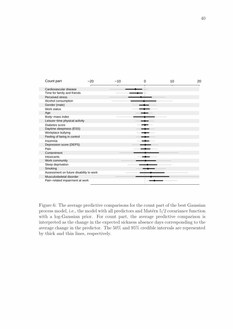
40

Cardiovascular diseaseTime for family and friendsPerceived stressAlcohol consumptionGender (male)Work statusAgeBody−mass indexLeisure−time physical activityDiabetes scoreDaytime sleepiness (ESS)Workplace bullyingFeeling of being in controlInsomniaDepression score (DEPS)PainContentmentIntoxicantsWork communitySleep deprivationSmokingAssessment on future disability to workMusculoskeletal disorderPain−related impairment at work

Count part −20 −10 0 10 20

Figure 6: The average predictive comparisons for the count part of the best Gaussianprocess model, i.e., the model with all predictors and Matern 5/2 covariance functionwith a log-Gaussian prior. For count part, the average predictive comparison isinterpreted as the change in the expected sickness absence days corresponding to theaverage change in the predictor. The 50% and 95% credible intervals are representedby thick and thin lines, respectively.

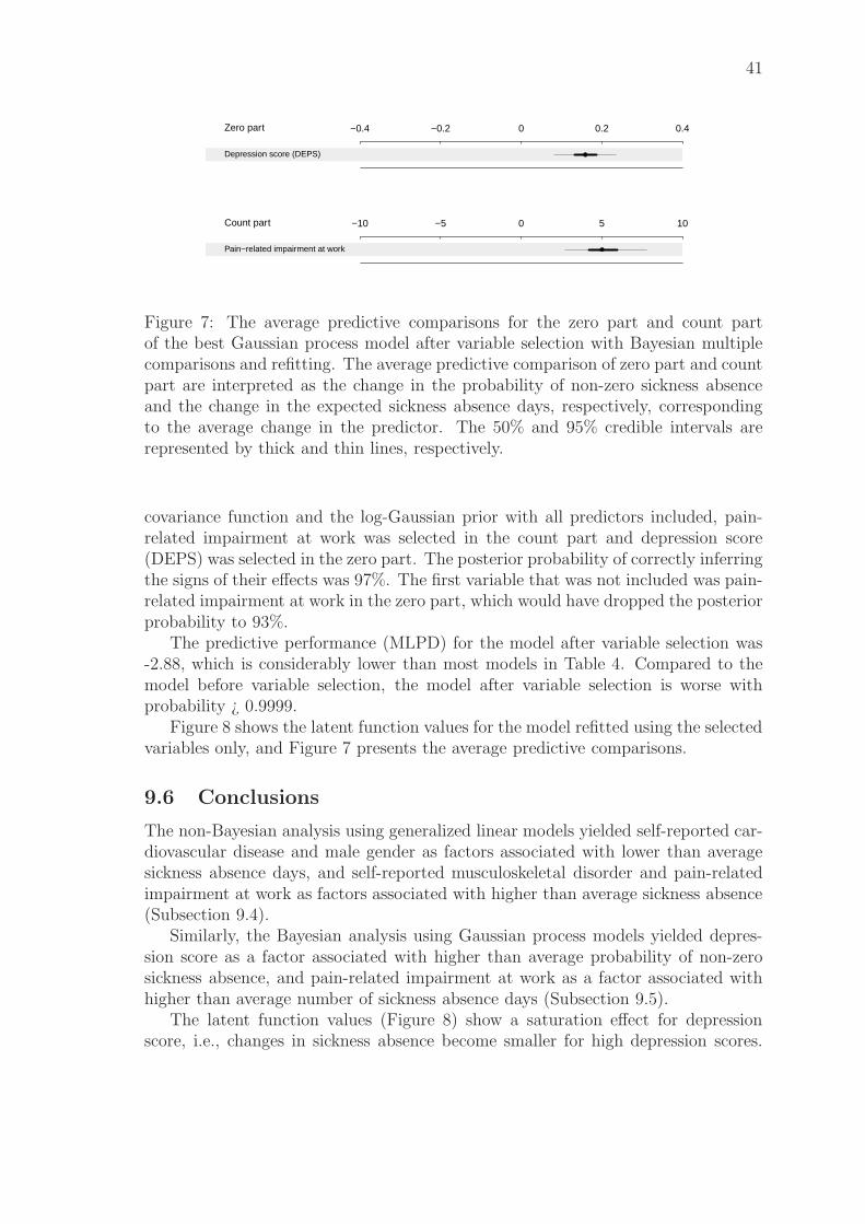
41

Depression score (DEPS)

Zero part −0.4 −0.2 0 0.2 0.4

Pain−related impairment at work

Count part −10 −5 0 5 10

Figure 7: The average predictive comparisons for the zero part and count partof the best Gaussian process model after variable selection with Bayesian multiplecomparisons and refitting. The average predictive comparison of zero part and countpart are interpreted as the change in the probability of non-zero sickness absenceand the change in the expected sickness absence days, respectively, correspondingto the average change in the predictor. The 50% and 95% credible intervals arerepresented by thick and thin lines, respectively.

covariance function and the log-Gaussian prior with all predictors included, pain-related impairment at work was selected in the count part and depression score(DEPS) was selected in the zero part. The posterior probability of correctly inferringthe signs of their effects was 97%. The first variable that was not included was pain-related impairment at work in the zero part, which would have dropped the posteriorprobability to 93%.

The predictive performance (MLPD) for the model after variable selection was-2.88, which is considerably lower than most models in Table 4. Compared to themodel before variable selection, the model after variable selection is worse withprobability ¿ 0.9999.

Figure 8 shows the latent function values for the model refitted using the selectedvariables only, and Figure 7 presents the average predictive comparisons.

9.6 Conclusions

The non-Bayesian analysis using generalized linear models yielded self-reported car-diovascular disease and male gender as factors associated with lower than averagesickness absence days, and self-reported musculoskeletal disorder and pain-relatedimpairment at work as factors associated with higher than average sickness absence(Subsection 9.4).

Similarly, the Bayesian analysis using Gaussian process models yielded depres-sion score as a factor associated with higher than average probability of non-zerosickness absence, and pain-related impairment at work as a factor associated withhigher than average number of sickness absence days (Subsection 9.5).

The latent function values (Figure 8) show a saturation effect for depressionscore, i.e., changes in sickness absence become smaller for high depression scores.

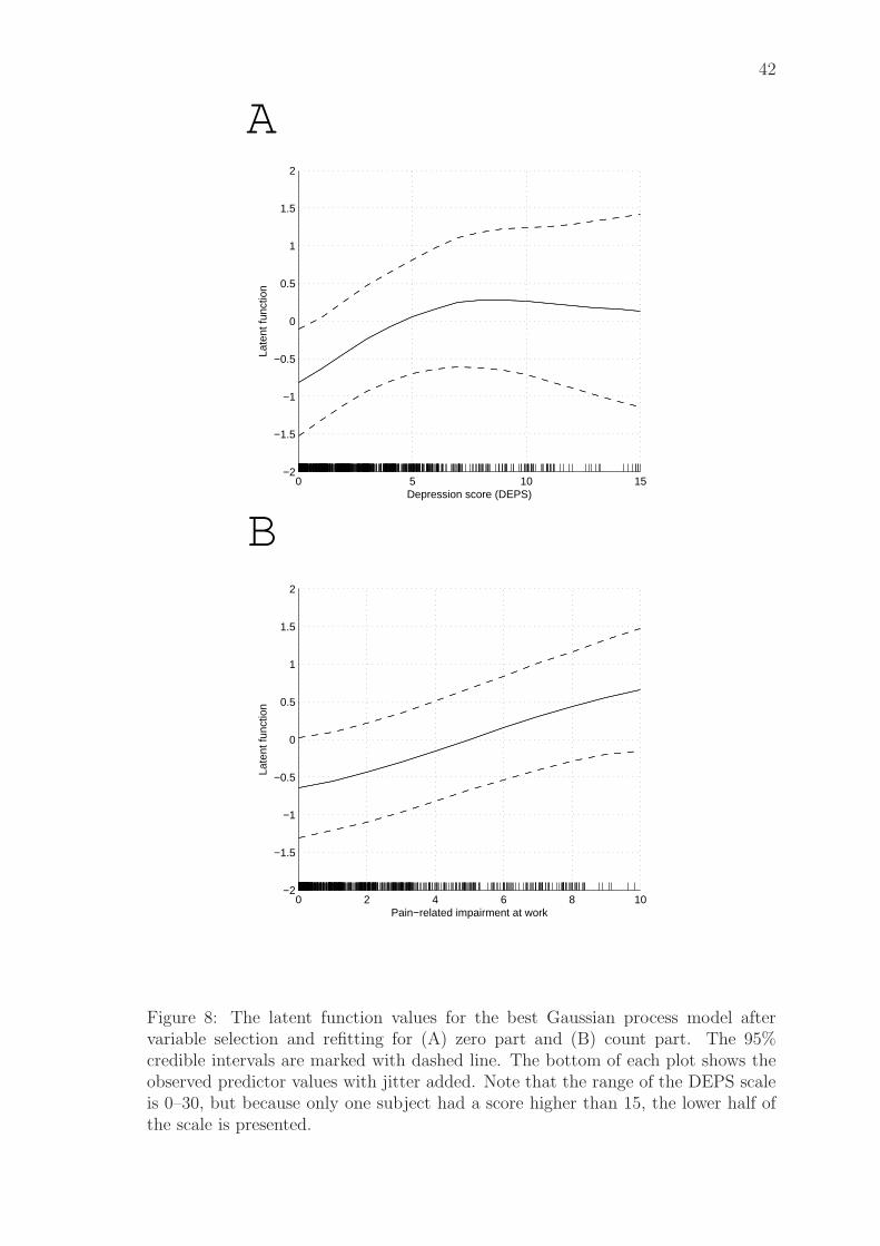
42

B

A

0 5 10 15−2

−1.5

−1

−0.5

0

0.5

1

1.5

2

Depression score (DEPS)

Late

nt fu

nctio

n

0 2 4 6 8 10−2

−1.5

−1

−0.5

0

0.5

1

1.5

2

Pain−related impairment at work

Late

nt fu

nctio

n

Figure 8: The latent function values for the best Gaussian process model aftervariable selection and refitting for (A) zero part and (B) count part. The 95%credible intervals are marked with dashed line. The bottom of each plot shows theobserved predictor values with jitter added. Note that the range of the DEPS scaleis 0–30, but because only one subject had a score higher than 15, the lower half ofthe scale is presented.

43

However, the effect might not reflect the actual relationship between depression andsickness absence, but instead be an artifact of too little data.

Predictors not included in the model after variable selection, presented in Fig-ures 7 and 8 may contain predictive information, but the data does not have enoughinformation to assess the sign of the effects with high certainty (probability higherthan 95%). At least some predictors that were not included in the model containuseful predictive information, as the predictive performance dropped from -2.75 to-2.88 when variable selection was done.

Also, using average predictive comparisons for variable selection may hide non-linear effects because average predictive comparisons considers only average changesover the whole population.

Bayesian multiple comparisons seems conservative in inferring the relevance ofpredictors. However, the threshold 95% used in Bayesian multiple comparisons isarbitrary, and lowering it would have included more predictors in the model.

44

10 Discussion

The predictors from both Gaussian process regression and generalized linear modelsgenerally agree with previous research. However, the association between cardio-vascular disease and a low rate of sickness absence found with the non-Bayesiangeneralized linear model has not been found in previous studies.

The current finding may be an artifact of a sample selection bias, which is causedby non-random participation to the underlying intervention study. Cardiovasculardisease was self-reported, so biased reporting might also contribute to the finding.Vascular diseases also include varices, which is not assumed to increase sicknessabsence, although not lower them either, but which might still confound the results.

Our Gaussian process models can probably be improved. For example, zero-inflated Gaussian process models might yield better predictive performance thanthe hurdle models, but we did not use them because of stability issues. Also, ap-proximating the latent posterior using expectation propagation instead of Laplaceapproximation is likely to yield better results. The forthcoming version of GPstufftoolbox has a more stable implementation of the expectation propagation algorithm,but it was not yet available during the writing of this Thesis.

Many predictors were partly redundant or overlapped, e.g., daytime sleepiness,insomnia, and sleep deprivation. For overlapping predictors, the total effect theyhave on sickness absence is distributed between them, which can cause each to beconsidered non-relevant separately and thus not included in the variable selection,although their common effect could be relevant. A factor analysis to discover latentpredictors or a careful preselection of the predictors lessen the problem but can hideunexpected effects, for example, in the hypothetical case that daytime sleepiness hasan effect on sickness absence that insomnia or sleep deprivation do not convey.

As noted in Section 5, Gaussian process models are well-suited for finding non-linear relationships between the predictors and the response variable and also inter-actions between the predictors. Based on Figure 8, it seems that there is a saturationeffect for depression. On the other hand, we did not find the specific non-linear re-lationships suggested, e.g., U-shaped relationship between alcohol use and sicknessabsence, suggested by Vahtera et al. (2002), or the interaction of gender and feelingoverloaded at work, found by Kivimaki et al. (2000). This may be due to themusing different models, or differences in the study population.

We did the data cleaning and checking painstakingly, so the data quality wasgood. However, modeling sickness absence is inherently difficult because the dis-tribution of sickness absence days is skewed and long-tailed. Future research couldtry new models to overcome these difficulties, e.g., as suggested by Taimela et al.(2007), a model with distinct parts for zero sickness absence, low rate of sicknessabsence, and high rate of sickness absence.

45

References

[1] Ala-Mursula, L. et al., 2002. Employee control over working times: associa-tions with subjective health and sickness absences. Journal of Epidemiology &Community Health, 56(4), 272–278.

[2] Bishop, C. M., 2006. Pattern Recognition and Machine Learning. New York:Springer.

[3] Berk, R., MacDonald, J. M., 2008. Overdispersion and Poisson Regression.Journal of Quantitative Criminology, 24(3), 269–284.

[4] Efron, B., 1979. Bootstrap methods: another look at the jackknife. The Annalsof Statistics, 7(1), 1–26.

[5] Duijts, S. F. et al., 2007. A meta-analysis of observational studies identifiespredictors of sickness absence. Journal of Clinical Epidemiology, 60(11), 1105–1115.

[6] Gelman, A., Carlin, J., Stern, H., Rubin, D., 1995. Bayesian Data Analysis.2nd ed. London: Chapman & Hall/CRC.

[7] Gelman, A., Hill, J., 2007. Data Analysis Using Regression and Multi-level/Hierarchical Models. Cambridge: Cambridge University Press.

[8] Gelman, A., Pardoe, I., 2007. Average predictive comparisons for models withnonlinearity, interactions, and variance components. Sociological Methodology,37(1), 23–51.

[9] Gelman, A., Tuerlinckx, F., 2000. Type S error rates for classical and Bayesiansingle and multiple comparison procedures. Computational Statistics, 15(3),373–390.

[10] Gelman, A., 2008. Scaling regression inputs by dividing by two standard devi-ations Statistics in Medicine, 27(15), 2865–2873.

[11] Kivimaki, M., Elovainio, M., Vahtera, J., 2000. Workplace bullying and sicknessabsence in hospital staff. Occupational and Environmental Medicine, 57(10),656–660.

[12] Kivimaki, M., et al., 2001. Sickness absence in hospital physicians: 2 year followup study on determinants. Occupational and Environmental Medicine, 58(6),361–366.

[13] Laaksonen, M., Martikainen, P., Rahkonen, O., Lahelma, E., 2008. Explana-tions for gender differences in sickness absence: evidence from middle-agedmunicipal employees from Finland. 65(5), 325–330.

[14] Lambert, D., 1992. Zero-inflated Poisson regression, with an application todefects in manufacturing. Technometrics, 34(1), 1–14.

46

[15] McCullagh, P., Nelder, J., 1989. Generalized Linear Models. 2nd ed. London:Chapman and Hall/CRC.

[16] Minka, T. P., 2001. Expectation propagation for approximate Bayesian infer-ence. UAI ’01: Proceedings of the 17th Conference in Uncertainty in ArtificialIntelligence, 362–369.

[17] Murphy, K., Dunham, M., 2008. PMTK: Probabilistic modeling toolkit. NeuralInformation Processing Systems (NIPS) Workshop on Probabilistic Program-ming.

[18] Niedhammer, I. et al., 1998. Psychosocial factors at work and sickness ab-sence in the Gazel cohort: a prospective study. Occupational and EnvironmentalMedicine, 55(11), 735–741.

[19] R Development Core Team, 2009. R: A language and environment for sta-tistical computing. Vienna: R Foundation for Statistical Computing. URLhttp://www.R-project.org/.

[20] Rasmussen, C. E., Williams, C. K. I., 2006. Gaussian Processes for MachineLearning. 2nd ed. Cambridge: MIT Press.

[21] Reijonsaari, K. et al., 2009. The effectiveness of physical activity monitoringand distance counselling in an occupational health setting - a research protocolfor a randomised controlled trial (CoAct). BMC Public Health, 9(1), p.494.

[22] Rubin, D. B., 1981. The Bayesian bootstrap. The Annals of Statistics 1981,9(1), 130–134.

[23] Taimela, S. et al., 2007. Self-reported health problems and sickness absence indifferent age groups predominantly engaged in physical work. Occupational andEnvironmental Medicine, 64(11), 739–746.

[24] Vanhatalo, J., Riihimaki, J., Hartikainen, J., Vehtari, A., 2011. Bayesian mod-eling with Gaussian processes using the MATLAB toolbox GPstuff, submitted.

[25] Vahtera, J. et al., 2002. Alcohol intake and sickness absence: a curvilinearrelation. American Journal of Epidemiology, 156(10), 969–976.

[26] Vehtari, A., Lampinen, J., 2002. Bayesian model assessment and comparisonusing cross-validation predictive densities.

[27] Venables, W. N. & Ripley, B. D., 2002. Modern Applied Statistics with S. 4thed. New York: Springer. Neural Computation, 14(10), 2439–2468.

[28] Virtanen, M. et al., 2007. Job strain and psychologic distress influence onsickness absence among Finnish employees. American Journal of PreventiveMedicine, 33(3), 182–7.

47

[29] Zeileis, A., Kleiber, C., Jackman, S., 2008. Regression models forcount data in R. Journal of Statistical Software, 27(8), 1–25. URLhttp://www.jstatsoft.org/v27/i08/.

48

A Priors

We present here a detailed account of the priors used for Gaussian process modelsin Section 9 and the lines of code used to implement them in MATLAB toolboxGPstuff (Vanhatalo et al., 2011).

For linear covariance function, we used a hierarchical prior of inverse chi-squareddistributions,

pc_s2 = prior_sinvchi2(’s2’, 0.01, ’nu’, 1);

pc = prior_sinvchi2(’s2’, 0.01, ’nu’, .1, ’s2_prior’, pc_s2);

The corresponding covariance function structure was initialized by

gp_cf = gpcf_linear(’coeffSigma2’, 0.02*ones(1,k), ’coeffSigma2_prior’, pc);

where k is the number of inputs to the regression.For neural network covariance function, a Student’s t distribution was used as

the prior for the square root of the weights,

pnn = prior_sqrtt(’s2’, 10^2);

gp_cf = gpcf_neuralnetwork(’weightSigma2’, ones(1,k), ’biasSigma2’, 1, ...

’weightSigma2_prior’, pnn);

Matern 5/2 and squared exponential covariance functions with the hierarchical priorused inverse chi-squared distributions,

pl_s2 = prior_sinvchi2(’s2’, 1, ’nu’, 1);

pl = prior_sinvchi2(’s2’, 1, ’nu’, .2, ’s2_prior’, pl_s2);

The log-Gaussian prior was initialized by

pl = prior_loggaussian(’s2’, 2, ’mu’, 1.6);

For both priors, a prior for the magnitude term was the Student’s t distribution forthe square root of the parameter,

pm = prior_sqrtt(’s2’, 4, ’nu’, 40);

The Matern 5/2 and squared exponential covariance function structures were ini-tialized by

gp_cf = gpcf_matern52(’lengthScale’, ones(1,k), ’magnSigma2’, .5, ...

’lengthScale_prior’, pl, ’magnSigma2_prior’, pm);

and

gp_cf = gpcf_sexp(’lengthScale’, ones(1,k), ’magnSigma2’, .2, ...

’lengthScale_prior’, pl, ’magnSigma2_prior’, pm);