Short-term forecasts of COVID-19 spread across Indian ...

1

Short-term forecasts of COVID-19 spread across Indian states until 29

May 2020 under the worst-case scenario

Neeraj Poonia1, Sarita Azad

2*

1 School of Basic Sciences, Indian Institute of Technology Mandi, 175075, India.

2 School of Basic Sciences, Indian Institute of Technology Mandi, 175075, India.

*Corresponding author [email protected]

Abstract

The very first case of corona-virus illness was recorded on 30 January 2020, in India and the number

of infected cases, including the death toll, continues to rise. In this paper,

we present short-term forecasts of COVID-19 for 28 Indian states and five union territories using real-

time data from 30 January to 20 May 2020. Applying Holt’s second-order exponential smoothing

method and autoregressive integrated moving average (ARIMA) model, we generated 10-day ahead

forecasts of the likely number of infected cases and deaths in India until 29 May 2020. Our results

show that the number of cumulative cases in India will rise to169109 [PI 95% (14426, 19455)],

concurrently the number of deaths may increase to 4863 [PI 95% (4221, 5551)] by 29 May 2020.

Further, we have marked the states (e.g. Delhi, Uttar Pradesh, Rajasthan, Madhya Pradesh,

Maharashtra, Gujarat, and Tamil Nadu) where outburst is expected by considering the cases above

three standard deviations. Under the worst-case scenario, Maharashtra is likely to be the most affected

state with around 62628 [PI 95% (52840, 73555)] cumulative cases by 29 May 2020. However,

Kerala and Karnataka are likely to remain in the lesser affected region. The presented results mark the

states where lockdown by 1 June 2020, can be loosened.

Keywords: COVID-19; India; Prediction models; Statistics; Data; Indian states.

1 Introduction

COVID-19 illness, an on-going epidemic, started in Wuhan city, China, in December 2019

continues to cause infections in many countries around the world [1]. Considering the scale

and speed of transmission of COVID-19, on 11 March 2020, the World Health Organization

(WHO) declared it as a pandemic [2]. Thereafter, COVID-19 has become a threat to human

life on the planet. It has shown rapid infections in almost all countries, and there is no cure

available for this deadly virus. Presently governments have issued precautionary measures

such as social distancing, sanitization of streets and markets, quarantine of suspected and

infected cases, and lockdown of the communities at different scales (colonies, towns, states,

and countries, etc.). In India, exponential growth has not been observed as compared to the

USA and other European countries. It is due to the measures taken by the Indian government.

It indicates that there is a strong influence of these measures, such as lockdown on the

transmission behavior of COVID-19. On the other side, these measures create substantial

economic losses to the communities, and hence actions mentioned above cannot be imposed

for longer periods. Mainly, developing countries (such as India) cannot afford such payoff

after some finite time. The Indian government has continuously reviewed every hour

situation in every state. The government has become more focused on localizing the

lockdown in particularly alarming states and few towns which are hotspots for COVID-19.

For all these, it is important to have short-term forecasts which can be steering point for

decision-makers and administrations. In this connection, data-based statistical models such as

Autoregressive integrated moving average (ARIMA) and Holts method have shown

effectiveness in predicting short-term forecast including the dengue fever [3, 4], the

Preprints (www.preprints.org) | NOT PEER-REVIEWED | Posted: 28 April 2020 doi:10.20944/preprints202004.0491.v1

© 2020 by the author(s). Distributed under a Creative Commons CC BY license.

https://doi.org/10.20944/preprints202004.0491.v1

http://creativecommons.org/licenses/by/4.0/

2

hemorrhagic fever with renal syndrome [5], Tuberculosis [6] and COVID-19 [7]. ARIMA

has more ability compared to other prediction models like the support vector machine and

wavelet neural network for drought forecasting [8]. Also, exponential smoothing methods

have been widely used for forecasting of the population in West Java [9], an inflation rate of

Zambia [10] including a prediction for epidemic mumps [11] and COVID-19 [12–17].

However, mainly, for India, the short-term forecast is not done thoroughly. As India has

diversity across the states, it will be essential to study the spreading behavior of COVID-19

in different Indian states. This article presents a short-term forecast for various Indian states

which are severely infected.

The main objective of the present paper is to present 10-day ahead forecasts from 21

to 29 May 2020 of the cumulative number of infected cases and deaths due to COVID-19.

This work also presents the analysis of Indian states at the regional level to understand the

spread of infection. The current situation of India is shown in Figure 1, with the cumulative

number of infected cases and deaths from 30 January to 20 May 2020.

Figure 1: (a) Number of infected cases from 30 January to 20 May 2020; (b) Number of

deaths from 30 January to 20 May 2020.

2 Materials and Methods

2.1ARIMAModel

The process whose statistical properties do not change with time, i.e. process with constant mean and

constant variance, known as a stationary process, is a crucial collection of stochastic processes.

Mathematically, the joint distribution of )(),...,( 1 ktXtX and )(),...,( 1 ktXtX is the same for all

kttt ,...,, 21 of a stationary process. Simply put, shifting the origin of time by a quantity does not

change the statistical properties of the process. Usually, dealing with real-time data, most time series

does not exhibit stationarity in nature as they have no fixed mean. The properties of the crucial

collection of models for which the thd difference of the time series is a stationary mixed

autoregressive moving average process (ARMA). These models are known as ARlMA models. The

ARMA model, introduced by Box and Jenkins, is the collection of popular methods that are directly

applicable to modeling and analyzing the time series [18]. The ARMA model is formed by the merger

of two models, the autoregressive AR(p) model and the moving average MA(q) model. These models

are directly applicable to time series with stationary behavior. In case the series is non-stationary, it

must be dealt via differencing to make it stationary. Generally, the ARMA model after differencing is

known as ARIMA (p, d,q). Addressing

t

d

t

d

t XkXH )1( (1)



3

The general ARIMA model is given by

qtqtptptt JJHHH ......11 (2)

Hence, the ARIMA model can be written as

tt JkgHkf )()( (3)

tt

d JkgXkf )()( (4)

The expressions in the Eq. 4 are defined as: )(),( kgkf are polynomials of degree p, q respectively s.t.

p

pkkkf ...1)( 1 (5)

and

q

qkkkg ...1)( 1 (6)

While, d is an operator, known as difference operator, and used to make the difference of time

series stationary; and d is the difference value. In real-time data, taking the first difference (d=1) is

usually found to be sufficient and occasionally second difference (d=2) would be enough to achieve

stationarity.

Akaike Information Criterion (AIC) is one of the essential criteria to select between competing

models. Mathematically,

AIC =T

p

T

eT

t

t2

log 1

(7)

The model which has the least AIC is selected as the best model. Autocorrelation functions (ACF)

and partial autocorrelation functions (PACF) are used to select order of moving average process

MA(q) and autoregressive process AR(p) respectively. In the process to investigate the stationarity of

time series Kwiatkowski–Phillips–Schmidt–Shin (KPSS) [19] and Augmented Dickey-Fuller (ADF)

[20] tests are used. To reject the null hypothesis, the p-value must be smaller than the significance

level.

2.2 Holt’sMethod The numbers of confirmed cases and deaths in India are increasing day by day, as shown in Figure 1

thereupon the time series exhibit trend. Simple exponential smoothing methods should not apply in

this case. When data shows the pattern, and there is no seasonality, Holt's method is a primary tool to

handle it. Holt's method is a double exponential smoothing method (not based on ARIMA approach)

which has two parameters. This method divides the time series into two sections: the level and the

trend denoted by tB and tM respectively. These two parts are as follows:

))(1( 11 tttt MBXB (8)

11 )1()( tttt MBBM (9)

The in-future forecasts values htX of the time series can be calculated by:

)(hMBX ttht (10)

whereh is the number of periods in the future. Diverse statistical meaning-making models in the R-

language platform were used to evaluate the time series of infected cases and deaths for prediction

purposes.

3. Results and Discussion



4

We present results for 10-day ahead forecasts ( May 20 to May 29, 2020) generated for the

cumulative number of infected cases and deaths in India as well as in the ten most affected

states: Kerala, Maharashtra, Delhi, Gujarat, Tamil Nadu, Telangana, Uttar Pradesh, Madhya

Pradesh, Karnataka, Rajasthan. In this work, we used two models Holt's method and ARIMA

model to forecast the cumulative infected cases and deaths of COVID-19. For the ARIMA

model, we forecast per day new infected case(s) and new death(s), whereas for Holt’s method

cumulative numbers are generated.

3.1 Validation: As of 22 April 2020, there were 21370 cumulative numbers of infected cases

and 681 cumulative numbers of deaths in India. For validation purposes, we forecasted the

cumulative number of infected cases and deaths from April 22 to May 1, 2020 using ARIMA

and Holt's method. Our forecasting results showed 36335 [PI 95% ((30884, 42918))]

cumulative number of infected cases using ARIMA(1,1,2) model and 36624 [PI 95% (30716,

43051)] cases using Holt's method (α=0.9, β=0.3), in both cases the 95% prediction intervals

includes the actual values. While forecasting results of the cumulative number of deaths are

1140 [PI 95% (945, 1354)] using Holt's method (α=0.8, β=0.2) and 1099 [PI 95% (959, 1553)]

using ARIMA(0,1,3) both the intervals includes the actual value, 1223 deaths by 1 May

2020, within 95% prediction interval. When necessary the Box-Cox transformation was used

to stabilize the variance in Holt's and ARIMA models.

3.2 India forecasting:

3.2.1 ARIMA model: During the analysis and forecasting of a time series, it is good to plot

the time series data and pay attention to the unique features exhibited by the time series. It

gives direction to the researcher for choosing an appropriate modeling approach that directly

captures identified features. Before starting the procedure, there is a need to make the time

series stationary. To stabilize the variance, we used square root transformation on the infected

number of cases per day time series. For investigating the stationarity of time series, we take

the support of the KPSS and ADF test, and results are shown in Table 1. The first difference

of series, i.e. d=1, is optimum to make series reasonably stationary. Based on a 5%

significance level both the tests, ADF and KPSS, reject the hypothesis of stationarity of time

series without making any difference. Afterwards taking the first difference, both the criteria

agree on the stationarity of time series. Further, to estimate another two parameters of the

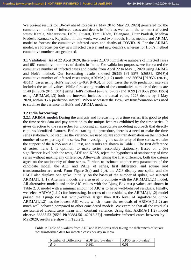
candidate model, the ACF and PACF of series, first difference, and square root

transformation are used. From Figure 2(a) and 2(b), the ACF display one spike, and the

PACF also displays one spike. Initially, on the bases of the number of spikes, we selected

ARIMA(1, 1, 1). Alternate models are also used to compete with the ARIMA(1,1,1) model.

All alternative models and their AIC values with the Ljung-Box test p-values are shown in

Table 2. A model with a minimal amount of AIC is to have well-behaved residuals. Finally,

we select ARIMA(1,1,2) for forecasting. In terms of the residuals, the ARIMA(1,1,2) model

passed the Ljung-Box test with p-values larger than 0.05 level of significance. Since

ARIMA(1,1,2) has the lowest AIC value, which means the residuals of ARIMA(1,1,2) are

much well behaved compared to other considered models. We examine that all the residuals

are scattered around zero mean with constant variance. Using this, ARIMA(1,1,2) model

observe 36335.53 [95% PI(30884.56 -42918.87)] cumulative infected cases between by 1

May2020, results are shown in Table 3.

Table 1: Table of p-values from ADF and KPSS tests after taking the differences of square

root transformed data for infected cases per day in India.

Number of Difference ADF test (p-value) KPSS test (p-value)

d=0 0.961 0.01



5

d=1 0.01 0.058

Table 2: Potential models for infected cases per day with AIC value and Ljung-Box test p-

value.

Model AIC value Ljung-Box test (p-value)

ARIMA (0,1,2) 427.77 0.263

ARIMA (1,1,2) 418.82 0.518

ARIMA (0,1,1) 428.05 0.341

ARIMA (1,1,1) 428.59 0.258

ARIMA (1,1,3) 420.72 0.438

Figure 2: (a) ACF for the infected number of cases per day after square root

transformation; (b) PACF for the infected number of cases per day after square root

transformation; (c) ACF for the number of deaths per day; (d) PACF for the number

of deaths per day.

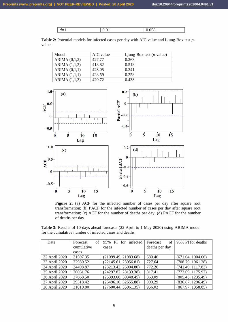
Table 3: Results of 10-days ahead forecasts (22 April to 1 May 2020) using ARIMA model

for the cumulative number of infected cases and deaths.

Date Forecast of

cumulative

cases

95% PI for infected

cases

Forecast of

deaths per day

95% PI for deaths

22 April 2020 21507.35 (21099.49, 21983.68) 680.46 (671.04, 1004.66)

23 April 2020 22980.52 (22145.61, 23956.81) 727.64 (708.79, 1061.28)

24 April 2020 24498.87 (23213.42, 26004.80) 772.26 (741.49, 1117.82)

25 April 2020 26061.76 (24297.82, 28133.38) 817.41 (773.69, 1175.92)

26 April 2020 27668.50 (25393.68, 30348.45) 863.09 (805.46, 1235.49)

27 April 2020 29318.42 (26496.10, 32655.88) 909.29 (836.87, 1296.49)

28 April 2020 31010.80 (27600.44, 35061.35) 956.02 (867.97, 1358.85)



6

29 April 2020 32744.95 (28702.47, 37570.28) 1003.28 (898.79, 1422.54)

30 April 2020 34520.13 (29798.33, 40187.84) 1051.06 (929.39, 1487.52)

1 May 2020 36335.63 (30884.56, 42918.87) 1099.38 (959.77, 1553.76)

Since only one difference makes the time series stationary, we conclude to take d=1. Results

of ADF and KPSS tests are presented in Table 4. From Figure 2(c) and 2(d), ACF

demonstrates two significant spikes, and PACF demonstrates zero significant spike. Based on

the number of spikes, we selected ARIMA (0, 1, 2). Alternate models were also used to

compete with the ARIMA (0,1,2) model. Details of other potential models along with AIC

values and Ljung-Box test p-values given in Table 5. Furthermore, to forecast the number of

deaths per day in India, we found ARIMA (0,1,3) a reasonable model among other

competitor models it has minimum AIC value. Furthermore, we found residuals are randomly

scattered around zero mean with non-changing variance with time. Also, ARIMA(0,1,3) does

not show a lack of fit with the Ljung-box test p-value larger than 0.05. Graphical results of

forecasting from infected cases and deaths are shown in Figure 3. Applying ARIMA(0,1,23),

1099.38 [95% PI(959.77-1553.76)] cumulative deaths are expected in coming 10 days in

India. Results for 10-day ahead forecast for per day infected cases, and deaths are shown in

Table 3. To eliminate the effect of square root transformation in per day infected cases we

take a square of forecasted observations.

Table 4: Table of p-values from ADF and KPSS tests for deaths per day in India.

Number of Difference ADF test (p-value) KPSS test (p-value)

d=0 0.979 0.01

d=1 0.01 0.058

Table 5: Potential models for deaths per day data with AIC values and Ljung-Box test p-

values.

Model AIC value Ljung-Box test (p-

value)

ARIMA (0,1,3) 497.32 0.408

ARIMA (1,1,4) 499.79 0.208

ARIMA (0,1,2) 498.10 0.248

ARIMA (1,1,2) 498.77 0.274

ARIMA (1,1,3) 498.41 0.365



7

Figure 3: (a)10-days ahead forecast (22 April to 1 May 2020) for the number of

infected cases per day using ARIMA(1,1,2) model; (b) 10-days ahead forecast (22

April to 1 May 2020) for the number of deaths per day using ARIMA(0,1,3) model;

(c) 10-days ahead forecast (22 April to 1 May 2020) using Holt's method for the

cumulative number of infected cases; (d) 10-days ahead forecast (22 April to 1 May

2020) for the cumulative number of days using Holt's method.

3.2.2 Holt's Method: The time series plot of the cumulative number of confirmed cases and

deaths for India is presented in Figure 1 exhibiting the trend in time series, but it does not

have a pattern of seasonality. As a result of the features shown by time series in Figure 1,

Holt’s method was selected in this study to accomplish a 10-day ahead forecast (May 20 to

May 29, 2020). Generally, a Holt method has two smoothing constants, α and β (their values

lie in range 0 and 1). The square root transformation is used to stabilize the variance in the

time series of infected cases. In the process to attain the optimal parameters we applied by

trial and error technique. Results are shown in Table 6 with the value of α, β, AIC, and

RMSE values. The best model is selected with the lowest AIC and RMSE values. With the

parameters, α=0.9 and β=0.3, obtained values of AIC and RMSE are 381.02 and 1.05,

respectively. For this model, Ljung-Box test p-value=0.468 which agrees that model does not

exhibit any lack of fit.

Using Holt's method, different values of α and β are tried to retrieve the optimum

forecast for cumulative deaths. The square root transformation is used to stabilize the

variance in the time series of deaths. The results of the trials are listed in Table 7 with AIC

and RMSE values. Smallest values of AIC=151.78 and RMSE=0.26 at α=0.8 and β=0.2 are

achieved. Subsequently, checking the Ljung-Box test p-value=0.109 we identify that model

does not lack of fit. Graphical results of forecasting from infected cases and deaths are

presented in Figure 3. From Table 8, 36624.43 [95% PI(30716.59-43051.56)] cumulative

infected cases and 1140.70 [ PI % (945.32-1354.42)] cumulative deaths are in India up-to 1

May2020.



8

Table 6: Selection process for parameters in Holt’s method to forecast the cumulative

number of infected cases in India.

𝛂 𝞫 AIC value RMSE

0.1 0.1 503.15 2.19

0.5 0.1 435.19 1.46

0.5 0.5 400.55 1.18

0.9 0.5 383.37 1.06

0.9 0.3 381.02 1.05

Table 7: Selection process for parameters in Holt’s method to forecast the cumulative

number of deaths.

𝛂 𝛽 AIC value RMSE

0.1 0.1 253.11 0.49

0.5 0.1 185.53 0.32

0.5 0.5 167.63 0.29

0.9 0.5 157.12 0.27

0.8 0.2 151.78 0.26

Table 8: Results of 10-days ahead forecasts (22 April to 1 May 2020) using Holt’s method

for the cumulative number of infected cases and deaths.

Date Forecast of

cumulative

infected

cases

95% PI for infected

cases

Forecast of

cumulative

deaths

95% PI for deaths

22 April 2020 21498.39 (20883.67, 22122.02) 685.95 (658.43, 714.02)

23 April 2020 22981.26 (21992.15, 23992.12) 730.79 (690.78, 771.94)

24 April 2020 24513.58 (23102.62, 25966.35) 777.06 (723.16, 832.91)

25 April 2020 26095.35 (24209.69, 28051.72) 824.75 (755.44, 897.10)

26 April 2020 27726.57 (25311.47, 30251.70) 873.86 (787.58, 964.62)

27 April 2020 29407.24 (26407.03, 32568.84) 924.39 (819.55, 1035.54)

28 April 2020 31137.36 (27495.78, 35005.34) 976.34 (851.32, 1102.92)

29 April 2020 32916.93 (28577.24, 37563.27) 1029.71 (882.88, 1187.82)

30 April 2020 34745.95 (29650.98, 40244.67) 1084.49 (914.22, 1269.30)

1 May 2020 36624.43 (30716.59, 43051.56) 1140.70 (945.32, 1354.42)

3.3 Indian states forecasting:

COVID-19 is spreading very fast in India. Locating the regions of most spread within India

will give insight for the lifting the lockdown which commenced on 25 March 2020. On the

regional level, this study shows the analysis for the cumulative number of cases but not

deaths due to the unavailability of data. A glimpse of the current situation of the increasing

number of cases in 10 states is given in Figure 4, certainly detectable that Maharashtra,

Gujarat, and Delhi are the most affected states in India till April 21, 2020. And Kerala is least

affected in our list of states. Time series starts from the date when the first case was reported

in the respective state.



9

Figure 4: Number of infections in the ten most affected Indian states by corona-virus as of 30

January to 20 May 2020.

3.3.1 ARIMA model: For forecasting purposes, using the ARIMA model, the number of

newly infected cases per day are analyzed instead of cumulative infected cases. To select the

optimum ARIMA model for each state, firstly each state's time series is made stationary by

taking differences. Next, we used ADF and KPSS tests to check stationarity. To stabilize the

variance of Delhi, Telangana, Uttar Pradesh, and Gujarat time series, cube root

transformations are used; later, one difference is enough to remove the trend. While to

stabilize the variance of Maharashtra, Karnataka and Rajasthan time series, square root and

square transformations are used, respectively. The same procedure is adopted for all the ten-

time series of infected cases per day. AIC values are used to select the best models, and the

model is chosen on the base of the smallest AIC value. Results of analysis for ARIMA

models are shown in Table 9. Analysis by ARIMA models shows that Maharashtra and

Gujarat will be the most affected states by 1 May 2020, with around 9787.24 and

4216cumulative cases, respectively. As we observe that Kerala's growth is declining and it

will be less affected states with 449 [PI 95%(408-574.99)] cumulative cases. All the models

passed the Ljung-Box test as well as does not show any lack of fit.

Table 9: Region-wise details of ARIMA models which were used for 10-days ahead forecasts

(22 April to 1 May 2020), along with AIC values and Ljung-Box test p-values. Point forecasts

and 95% prediction intervals are given in the last two columns.

Region ARIMA

Model

AIC

value

Ljung-Box

test

Point

forecast for

95% PI for infected

cases



10

3.3.2 Holt's method: Square root transformation is used to stabilize the variance of

Rajasthan, Maharashtra, Karnataka,and Uttar Pradesh. The cube root and square

transformation are used for Delhi, Kerala, Telangana, and Gujarat, respectively. Summary of

Holt's method display that Maharashtra and Delhi will be most affected states with around

9768.91 and 3768.39cumulative number of infected cases, respectively. Meanwhile, Kerala

will be the less affected state in our list with about 451.67 cumulative number of infected

cases. The selection of optimum Holt's method is performed using the minimum values of

AIC and RMSE. Although, all the model passed the Ljung-Box test, which state that model

does not show any lack of fit. Results of the forecast for each state are given in Table 10 with

Ljung-Box test p-values. The final graphical results of the analysis using both the models,

ARIMA model, and Holt's method, are shown in Figures 5-11.

Table 10: Region-wise 10-days ahead forecasts (22 April to 1 May 2020) details of Holt's

method, along with Ljung-Box test p-values. Point forecast and 95% prediction intervals are

given in the last two columns.

Region Ljung-Box test

(p-value)

Point forecast

for infected

cases

95% PI for infected

cases

Kerala 0.134 451.67 (408, 858.58)

Maharashtra 0.776 9768.91 (7453.81, 12396.63)

Rajasthan 0.073 2978.53 (1921.79, 4265.86)

Delhi 0.051 3768.39 (2081, 6607)

Telangana 0.029 1424.42 (919, 3171.29)

Karnataka 0.166 602.05 (495.65, 708.44)

Gujarat 0.229 3562.28 (2992.38, 4052.81)

Uttar Pradesh 0.138 2569.51 (1773.49, 3512.69)

Tamil Nadu 0.635 2158.51 (1664.95, 2652.07)

Madhya Pradesh 0.162 2301.68 (1540, 3321.74)

3.4 Recommendations on Lockdown Extension: India comprises 28 states and eight union

territories. Here we have analyzed all the states, including five union territories. In Figure 12, the

spatial distribution of coronavirus outbreak shows eight states in the red zone (extremely affected),

namely, Delhi, Rajasthan, Uttar Pradesh, Maharashtra, Telangana, Karnataka, Kerala, Tamil Nadu.

Similarly, seven states in the blue zone (intermediate affected), are Jammu & Kashmir, Punjab,

Haryana, Gujarat, Madhya Pradesh, Andhra Pradesh, West Benga. The green and light green (least

affected) zones include Himachal Pradesh, Uttrakhand, Bihar, Jharkhand, Chhattisgarh, Odisha,

Sikkim, Arunachal Pradesh, Assam, Nagaland, Manipur, Mizoram, Tripura, Meghalaya, Goa. To

construct the zones, we have divided the cumulative cases of states into quartiles as on 1 April 2020.

(p-value) infected

cases

Kerala (2,1,0) 498.53 0.329 449.38 (408, 574.90)

Maharashtra (0,1,2) 233.65 0.807 9787.24 (6949.81, 13757.06)

Rajasthan (0,1,1) 947.38 0.147 2741.40 (2305.22, 3053.91)

Delhi (1,1,2) 177.46 0.064 3039.73 (2139.72, 6085.18)

Telangana (2,1,0) 133.99 0.112 1321.37 (940.84, 2740.89)

Karnataka (3,1,0) 160.03 0.371 565.74 (419.09, 945.45)

Gujarat (0,1,0) 89.76 0.131 4216.00 (2216.24, 13118.90)

Uttar Pradesh (2,1,1) 140.25 0.161 2652.21 (1612. 43,4891.99)

Tamil Nadu (1,1,1) 440.69 0.840 2157.35 (1520, 2878.82)

Madhya Pradesh (0,1,1) 340.62 0.961 2281.84 (1540, 3688.99)



11

The same procedure is carried out for forecasted cumulative cases until 1 May 2020. As infected

cases are increasing, it is essential to notice which of the states will shift their zone.

Figure 13 shares Delhi, Rajasthan, Uttar Pradesh, Gujarat, Madhya Pradesh, Maharashtra, Telangana,

Tamil Nadu in the red zone and Jammu & Kashmir, Punjab, Haryana, Kerala, Karnataka, West

Bengal in the blue zone while Himachal Pradesh, Goa, Uttrakhand, Bihar, Jharkhand, Chhattisgarh,

Odisha, Sikkim, Assam, Arunachal Pradesh, Nagaland, Manipur, Mizoram, Tripura, Meghalaya are in

green and light green zones.

It is found that Kerala and Karnataka were in the red zone, and Gujarat and Madhya Pradesh

were in the blue area until 1 April 2020 (Figure 12). But they are likely to change their positioning by

1 May. Accordingly, Kerala and Karnataka will shift to the blue zone as cases are declining in both

states. Conversely, Gujarat and Madhya Pradesh will move to the red area. Recent 10 days ahead

forecast from 20 May to 29 May 2020 show that there will outburst of infected cases in seven Indian

states all the seven states are in the list of most affected states. Forecasting results of all the states by

29 May 2020 are shown in Table 11 along with outburst expected states. The government should

impose extra precautions in these states, as the cases will significantly rise in both in the coming days.

While lockdown should remain in the red zone, conversely, the blue area is not remarkably affected

by COVID-19, so lockdown should be lifted with some restrictions. It is advisable to lift the

lockdown in states within green and light green zones for the proper functioning of the economy.

Also, we divided the states based on cumulative cases that lie in one, two, and three standard

deviations from the overall mean (taken over all the states of India). Based on which we conclude that

states which have cases more than three standard deviations are expected to face outburst of infected

cases by 29 May 2020. While the states with cumulative cases lesser than one standard deviation will

be less affected by COVID-19 as shown in figure 14. Percentage error of validation for India and ten

most affected states shown in Table 12. Holt's method gives a 1.96% error for cumulative infected

cases of India which more precise than the ARIMA model. While for Rajasthan, Maharashtra,

Telangana, Gujarat, and Karnataka ARIMA model gives more precise results compare to Holt's

method.

Further, analysis of red and blue zones at the regional level is of importance to decide about

raising the district wise lockdown.

Table 11: 10 days ahead forecast for Indian states from May 20 to May 29, 2020.

State

Point

Forecast Lower Bound Upper Bound Mean SD

Kerala 826 723 930 214.0089286 220.4974513

Maharashtra 62628 52840 73555 4898.6875 8954.145967

Rajasthan 9336 5845 14198 1001.517857 1548.865758

Delhi 15337 12595 18349 1648.410714 2739.833994

Telangana 2037 1634 2471 403.8482143 518.2371924

Karnataka 2354 1934 2814 243.1785714 340.1449139

Gujarat 17164 13580 21167 1805.160714 3217.772739

Uttar Pradesh 7059 5880 8346 870.4107143 1348.852489

Tamil Nadu 19777 13954 26613 1567.044643 2954.255188

Madhya

Pradesh 7876 5864 10184 965.2678571 1506.346418

Haryana 1303 1026 1614 175.7857143 262.4089865

Himachal

Pradesh 149 92 252 18.33928571 24.45939955

Jammu &

Kashmir 1902 1610 2219 252.1160714 364.3831205

Punjab 2195 2002 6378 332.25 623.1226724

Uttarakhand 195 151 240 23.05357143 28.76209946

Bihar 3071 1779 4872 173.0446429 328.291191

Jharkhand 373 277 489 37.78571429 63.72949995



12

Chhattisgarh 134 101 186 18.47321429 24.85995362

Odisha 2150 1104 3707 91.40178571 193.9879935

Andhra

Pradesh 3187 2532 4235 516.2053571 769.7394334

West Bengal 4574 3911 5309 409.3660714 750.7096222

Assam 736 185 1650 20.27678571 28.71895812

Manipur 27 11 49 1.160714286 1.568574101

Tripura 210 173 399 18.72321429 48.151265

Meghalaya 13 13 19 3.8125 5.604906554

Arunachal

Pradesh 1 1 1 0.428571429 0.497095813

Pondicherry 24 18 37 3.794642857 4.540386126

Goa 245 143 374 4.339285714 6.84388801

Chandigarh 292 200 425 34.01785714 58.51387487

Mizoram 1 1 1 1 0

525.0970238

(Overall Mean)

1775.322896

(Overall SD)

Table 12: Percentage error of cumulative numbers of cases for India and ten most effect states using

both the method, ARIMA model and Holt's method, shown.

Forecasted Values Percentage Error

Location Actual Values ARIMA

model

Holt's

method

ARIMA

model

Holt's

method

India 37257 36335 36624 2.47 1.96

Kerala 497 779 451 9.65 9.25

Maharashtra 10498 9787 9768 6.77 6.95

Rajasthan 2584 2741 2978 6.07 15.24

Delhi 3515 3039 3768 13.54 7.19

Telangan 1039 1321 1424 27.14 37.05

Karnataka 576 565 602 1.90 4.51

Gujarat 4395 4216 3562 4.07 18.95

Uttar Pradesh 2281 2652 2569 16.26 12.62

Tamil Nadu 2323 2157 2158 7.14 7.10

Madhya

Pradesh

2719 2281 2301 16.10 15.37

4 Conclusions

The spread of the COVID-19 epidemic has been slow in India as compared to other countries

like Italy and the USA. It reflects the influence of the broad spectrum of social distancing

measures put in use by the government of India, which has played the role of a barrier to

growing infected cases and deaths, apparently helped to slow down the epidemic growth. Our

short-term forecast reveals that at the regional level, Delhi, Rajasthan, Gujarat, Maharashtra,

Uttar Pradesh, Madhya Pradesh and Tamil Nadu will be the most affected states in the

coming days which is confirmed by both quartile and standard deviation procedures as shown

in Figures 13-14. Considering the situation, lockdown should not be lifted in these states. The

number of cases in Kerala and Karnataka are found to be reducing. Moreover, these states are

shifted from the red zone to blue. Since very little growth in the future is predicted, lockdown

may be lifted in these states with some restrictions for the proper functioning of economic

activities. While states in green and light green zones, namely, Himachal Pradesh, Goa,

Uttrakhand, Bihar, Jharkhand, Chhattisgarh, Odisha, Sikkim, Assam, Arunachal Pradesh,

Nagaland, Manipur, Mizoram, Tripura, Meghalaya show very less growth in the infected



13

cases till 1 May, therefore, lockdown may be uplifted there. On India level, there will be

around 169109 [95% PI(144426, 196455)] cases and 4863 [95% PI(4221, 5551)] deaths up to

29 May 2020. The forecasts presented here are based on the assumption that current

mitigation efforts will continue.

Figure 5: (a) 10-days ahead forecast (22 April to 1 May 2020) using Holt's Method

for Kerala; (b) 10-days ahead forecast (22 April to 1 May 2020) using Holt's Method

for Rajasthan; (c) 10-days ahead forecast (22 April to 1 May 2020) using Holt's

Method for Delhi; (d) 10-days ahead forecast (22 April to 1 May 2020) using Holt's

Method for Madhya Pradesh.



14

Figure 6: (a) 10-days ahead forecast (22 April to 1 May 2020) using Holt's Method

for Tamil Nadu;(b) 10-days ahead forecast (22 April to 1May 2020) using Holt's

Method for Karnataka.

Figure 7: (a)10-days ahead forecast (22 April to 1 May 2020) using Holt's Method

for Uttar Pradesh; (b) 10-days ahead forecast (22 April to 1 May 2020) using Holt's

Method forTelangana.

Figure 8:(a) 10-days ahead forecast (22 April to 1 May 2020) using ARIMA(2,1,0) model

for Kerala; (b) 10-days ahead forecast (22 April to 1 May 2020) using ARIMA(0,1,1)

model for Rajasthan; (c) 10-days ahead forecast (22 April to 1 May 2020) using

ARIMA(1,1,2) model for Delhi; (d) 10-days ahead forecast (22 April to 1 May 2020) using

ARIMA(0,1,1) model for Madhya Pradesh.



15

Figure 9:(a) 10-days ahead forecast (22 April to 1 May 2020) using ARIMA(2,1,1) model

for Uttar Pradesh; (b) 10-days ahead forecast (22 April to 1 May 2020) using ARIMA(2,1,0)

model for Telangana; (c) 10-days ahead forecast (22 April to 1 May 2020) using

ARIMA(1,1,1) model for Tamil Nadu; (d) 10-days ahead forecast (22 April to 1 May 2020)

using ARIMA(3,1,0) model for Karnataka.

Figure 10: (a) 10-days ahead forecast (22 April to 1 May 2020) using

ARIMA(0,1,0) model for Gujarat; (b) 10-days ahead forecast (22 April to 1

May 2020) using ARIMA(0,1,2) model for Maharashtra.



16

Figure 11: (a) 10-days ahead forecast (22 April to 1 May 2020) using Holt's Method for

Gujarat; (b) 10-days ahead forecast (22 April to 1 May 2020) using Holt's Method for

Maharashtra.

-

Figure 12:Spatial distribution of the coronavirus outbreak in the period of 30 Jan to 1 April

2020.



17

Figure 13:Spatial distribution of the coronavirus outbreak in the period of 30 Jan to 1 May 2020.

Figure 14: Expected numbers of cases in Indian states by May 29, 2020.

5 Data Availability



18

We obtained daily updates of the cumulative number of infected cases and deaths of the corona-virus

illness for India from the Worldometer website (online available:

https://www.worldometers.info/corona-virus/country/india/). To obtain the state-wise cumulative

number of infected cases and deaths for the corona-virus illness we used the government of India

website (online available: https://www.mygov.in/corona-data/covid19-statewise-status). We

gathered data of infected case(s) every day at midnight (GMT-5) from 30 January to 21 April 2020.

And forecasted the cumulative number of infected cases and deaths of the epidemic over the India and

the cumulative number of infected cases in ten Indian states: Kerala, Maharashtra, Delhi, Gujarat,

Tamil Nadu, Telangana, Uttar Pradesh, Madhya Pradesh, Karnataka, and Rajasthan, which show a

high burden of COVID-19 cases.

6 Conflicts of Interest

The authors declare no conflicts of interest.

7 FundingStatement Research Support is provided by the Indian Institute of Technology Mandi.

References

[1]Roosa, K., Lee, Y., Luo, R., Kirpich, A., Rothenberg, R., Hyman, J.M., Yan, P. and Chowell, G.,

2020. Short-term Forecasts of the COVID-19 Epidemic in Guangdong and Zhejiang, China: February

13–23, 2020. Journal of Clinical Medicine, 9(2), p.596.

[2]Elmousalami, H.H. and Hassanien, A.E., 2020. Day Level Forecasting for corona-virus Disease

(COVID-19) Spread: Analysis, Modeling and Recommendations. arXiv preprint arXiv:2003.07778.

[3] Luz, P.M., Mendes, B.V., Codeço, C.T., Struchiner, C.J. and Galvani, A.P., 2008. Time series

analysis of dengue incidence in Rio de Januaryeiro, Brazil.The American journal of tropical medicine

and hygiene, 79(6), pp.933-939.

[4]Wongkoon, S., Jaroensutasinee, M. and Jaroensutasinee, K., 2012.Development of temporal

modeling for prediction of dengue infection in Northeastern Thailand.Asian Pacific journal of tropical

medicine, 5(3), pp.249-252.

[5] Liu, Q., Liu, X., Jiang, B. and Yang, W., 2011. Forecasting incidence of hemorrhagic fever with

renal syndrome in China using ARIMA model.BMC infectious diseases, 11(1), p.218.

[6] Rios, M., Garcia, J.M., Sanchez, J.A. and Perez, D., 2000. A statistical analysis of the seasonality

in pulmonary tuberculosis.European journal of epidemiology, 16(5), pp.483-488.

[7]ABenvenuto, D., Giovanetti, M., Vassallo, L., Angeletti, S. and Ciccozzi, M., 2020. Application of

the ARIMA model on the COVID-2019 epidemic dataset.Data in brief, p.105340.

[8] Zhang, Y., Yang, H., Cui, H. and Chen, Q., 2019. Comparison of the Ability of ARIMA, WNN

and SVM Models for Drought Forecasting in the Sanjiang Plain, China.Natural Resources Research,

pp.1-18.

[9]Supriatna, A., Susanti, D. and Hertini, E., 2017, January.Application of Holt exponential

smoothing and ARIMA method for data population in West Java. In IOP Conference Series:

Materials Science and Engineering (Vol. 166, No. 1, p. 012034). IOP Publishing.

[10]Jere, S. and Siyanga, M., 2016. Forecasting inflation rate of Zambia using Holt’s exponential

smoothing. Open journal of Statistics, 6(2), pp.363-372.


https://www.worldometers.info/corona-virus/country/india/

https://www.mygov.in/corona-data/covid19-statewise-status


19

[11] Shi, Y.P. and Ma, J.Q., 2010. Application of exponential smoothing method in prediction and

warning of epidemic mumps.Zhongguoyimiao he mianyi, 16(3), pp.233-237.

[12] Gupta, R. and Pal, S.K., 2020. Trend Analysis and Forecasting of COVID-19 outbreak in

India.medRxiv.

[13]Roosa, K., Lee, Y., Luo, R., Kirpich, A., Rothenberg, R., Hyman, J.M., Yan, P. and Chowell, G.,

2020. Real-time forecasts of the COVID-19 epidemic in China from February 5th to February 24th,

2020.Infectious Disease Modelling, 5, pp.256-263.

[14] Singh, R. and Adhikari, R., 2020. Age-structured impact of social distancing on the COVID-19

epidemic in India.arXiv preprint arXiv:2003.12055.

[15] Liu, Z., Magal, P., Seydi, O. and Webb, G., 2020. Predicting the cumulative number of cases for

the COVID-19 epidemic in China from early data.arXiv preprint arXiv:2002.12298.

[16] Liu, Z., Magal, P., Seydi, O. and Webb, G., 2020. Predicting the cumulative number of cases for

the COVID-19 epidemic in China from early data.arXiv preprint arXiv:2002.12298.

[17] Tariq, A., Lee, Y., Roosa, K., Blumberg, S., Yan, P., Ma, S. and Chowell, G., 2020. Real-time

monitoring the transmission potential of COVID-19 in Singapore, February 2020.medRxiv.

[18] Box, G.E., Jenkins, G.M., Reinsel, G.C. and Ljung, G.M., 2015. Time series analysis: forecasting

and control. John Wiley & Sons.

[19] Kwiatkowski, D., Phillips, P.C., Schmidt, P. and Shin, Y., 1992. Testing the null hypothesis of

stationarity against the alternative of a unit root.Journal of econometrics, 54(1-3), pp.159-178.

[20] Said, S.E. and Dickey, D.A., 1984. Testing for unit roots in autoregressive-moving average

models of unknown order.Biometrika, 71(3), pp.599-607.



Short-term forecasts of COVID-19 spread across Indian ...

Documents

Transcript of Short-term forecasts of COVID-19 spread across Indian ...