Short sale constraints, divergence of opinion and asset values: Evidence from the laboratory*

Gerlinde Fellner

Erik Theissen**

First version: November 2005

This version: March 1, 2006

Abstract: The overvaluation hypothesis (Miller 1977) predicts that a) stocks are overvalued when there are short selling restrictions and that b) the overvaluation is increasing in the degree of divergence of opinion. We design an experiment that allows us to test these predictions in the laboratory. Our results support the hypothesis that prices are higher in the presence of short selling constraints. The overvaluation does not depend on the degree of divergence of opinion.

JEL classification: C92, G14

Keywords: overvaluation hypothesis, short selling constraints, divergence of opinion

* We thank Rouhollah Mohammadi for valuable research assistance. Financial support from Deutsche Forschungs-gemeinschaft through SFB/TR 15 is gratefully acknowledged. ** Gerlinde Fellner and Erik Theissen, University of Bonn, BWL I, Adenauerallee 24-42, 53113 Bonn, Germany, email: fellner@uni-bonn.de and theissen@uni-bonn.de, respectively.

2

1 Introduction

If traders have different opinions about the value of an asset, optimists will buy and

pessimists will sell. Short sale restrictions prevent traders not currently owning an asset from

selling it and thus exclude pessimistic traders from the market. The marginal traders' assess-

ments of the asset value will thus be above average. If the price reflects these optimistic as-

sessments the asset will be overvalued, and the overvaluation will increase in the degree of

divergence of opinion. This is the overvaluation hypothesis first put forward by Miller (1977).

Although it is obviously incompatible with a rational expectations equilibrium (Diamond and

Verrecchia 1987) it has received much attention (and a fair amount of empirical support) in the

literature. A first wave of empirical studies dates from the 1980s and early 1990s. Interest in

the issue has been re-sparked recently, partially motivated by the question whether short-

selling constraints have contributed to the internet bubble of the late nineties.

The empirical results, to be summarized briefly in section 2, are inconclusive. Papers

relating short sale constraints for individual stocks to their valuation or their subsequent return

on balance find evidence in favor of the overvaluation hypothesis (yet not unanimously).

Charoenrook and Daouk (2005) who compare stock returns in countries with and without short

sale restrictions reject the overvaluation hypothesis. A possible explanation for these contradic-

tory results is the fact that empirical research into the issue is complicated by a number of im-

pediments. Most importantly, neither the value of a stock nor the degree to which it is short

sale constrained is directly observable. The same applies to the degree of divergence of opin-

ion. Consequently, researchers have to rely on proxies for all variables of interest. These prox-

ies may be noisy or even biased, and they may be correlated with other stock characteristics

that affect valuation.

3

Our paper contributes to the literature in that it provides the first experimental test of

the overvaluation hypothesis. None of the problems alluded to above is present in the labora-

tory. The experimenter controls the information structure and, consequently, the degree of di-

vergence of opinion. Similarly, short sale constraints are imposed by the experimenter. As

identical assets are traded with and without constraints, it is feasible to directly compare the

market value of the assets, rather than inferring overvaluation from proxy variables or subse-

quent returns.

Although the impact of short sale constraints on valuation is easily amenable to ex-

perimental research, we know of only three papers that vary the level of short selling con-

straints in the laboratory (King et al. 1993, Ackert et al. 2002 and Haruvy and Noussair 2005).

The design of these experiments differs from ours in a number of important ways. All three

papers were inspired by experimental results suggesting that bubbles occur frequently in ex-

perimental markets for long-lived assets (Smith et al. 1988). Against this background they test

whether allowing short sales has an impact on the frequency and magnitude of bubbles. The

experiments of King et al. 1993, Ackert et al. 2002 and Haruvy and Noussair 2005 feature sub-

jects with symmetric information. There is thus no divergence of opinion.1 Consequently, none

of these papers can be considered a test of Miller's (1977) overvaluation hypothesis because

there, divergence of opinion is a necessary condition for overvaluation to occur. Further, the

degree of divergence of opinion can obviously not be varied in a symmetric information set-

ting.

1 There may be differences of opinion due to strategic uncertainty, i.e., uncertainty with respect to the behaviour of other subjects. Strategic uncertainty is, however, not under the control of the experimenter.

4

The results of our experiments provide only partial support for the overvaluation hy-

pothesis. Prices in the experimental markets are higher when short selling is prohibited. The

overvaluation does, however, not depend on the degree of divergence of opinion.

The remainder of the paper is organized as follows. The next section presents a brief

summary of the literature. In section 3 we describe the experimental design and procedures.

Section 4 presents the hypotheses while the results are contained in section 5. In section 6 we

summarize our results and offer concluding remarks

2 Literature

As noted in the introduction the overvaluation hypothesis was first put forward by

Miller (1977). If traders in financial markets have different opinions, optimists will buy and

pessimists will sell. Short sale constraints prevent those pessimists not currently owning the

asset from selling it. Optimistic opinions will then be overweighted in market prices. Conse-

quently, short sale restrictions lead to overvaluation and the overvaluation is increasing in the

degree of divergence of opinion.

The overvaluation hypothesis as put forward by Miller (1977) is inconsistent with a ra-

tional expectations equilibrium.2 Diamond and Verrecchia (1987) present a rational expecta-

tions model in which short sale constraints do not lead to overvaluation but reduce the speed at

which new information, and bad information in particular, is incorporated into prices. Similar

results, though in a very different context, are derived in Hong and Stein (2003). Recent theo-

retical research has revived the overvaluation hypothesis. Duffie et al. (2002) derive a model in

5

which short sale constraints together with divergence of opinion (modeled by assuming differ-

ent priors about the payoff distribution) may lead to overvaluation. In the model of Johnson

(2004) higher degrees of divergence of opinion lead to lower subsequent returns in a fully ra-

tional context. In Scheinkman and Wei (2003) overconfidence creates divergence of opinion

and may, in the presence of short sale constraints, lead to overvaluation. A similar result is

derived in Jiang (2005).

Researchers have used various avenues in order to empirically test the overvaluation

hypothesis. The most common approach is to consider a cross-section of stocks and to test

whether stocks that are subject to short selling constraints are overvalued, and whether over-

valuation depends on the degree of divergence of opinion. This requires (a) identification of

stocks that are short sale constrained, (b) a measure for the degree of divergence of opinion3

and (c) a measure of asset value to identify overvaluation.

Various measures have been employed to identify short sale constrained stocks. These

include the short interest (Figlewski and Webb 1993, Asquith and Meulbroek 1996, Dechow et

al. 2001, Desai et al. 2002, Asquith et al. 2005, Boehme et al. 2005, Cohen et al. 2005), institu-

tional ownership (Asquith et al. 2005, Nagel 2005), the availability of options on the stock

(Figlewski and Webb 1993, Danielsen and Sorescu 2001, Mayhew and Mihov 2004, Boehme

et al. 2005), the inclusion of a stock in the "threshold list" (Diether et al. 2005) and the rebate

rate (Jones and Lamont 2002, Reed 2003, Ofek et al. 2004, Boehme et al. 2005, Cohen et al.

2 It is fair to note that Miller (1977) was well aware of the limitations of his model. He explicitly refers to the winner's curse problem and argues (p. 1158) that "many investors are still following naive procedures". 3 D'Avolio (2002) documents that a stock is more likely to be "on special" (i.e., to be expensive to short) when the degree of divergence of opinion is large. This suggests that the two explanatory variables of interest may not be independent.

6

2005). The most widespread proxy for the degree of divergence of opinion is the standard de-

viation of analyst forecasts (Diether et al. 2002, Boehme et al. 2005), but the standard devia-

tion of returns and the turnover ratio have also been employed (Boehme et al. 2005).

Some researchers identify overvalued stocks by analyzing valuation ratios (Dechow et

al. 2001, Desai et al. 2002, Jones and Lamont 2002) or by considering adjustments to analysts'

earnings forecasts (Francis et al. 2005). The most widespread approach is to rely on subsequent

returns to identify overvalued stocks. This approach is based on the implicit assumption that

either short sale constraints are removed or the divergence of opinion is reduced (e.g. because

new information is released), leading to a decrease of the level of overvaluation. Negative re-

turns are thus taken as evidence of initial overvaluation.

Given the measurement problems and the different approaches to resolve them, it is not

surprising that the conclusions are not entirely unanimous. A majority of papers find results

that are supportive of the overvaluation hypotheses (e.g. Figlewski and Webb 1993, Danielsen

and Sorescu 2001, Dechow et al. 2001, Desai et al. 2002, Diether et al. 2002, Jones and La-

mont 2002, Gopalan 2003, Ofek et al. 2004, Boehme et al. 2005, Cohen et al. 2005 and Nagel

2005). Additional evidence in favor of the overvaluation hypothesis is provided by Aitken et

al. (1998) and Chang and Yu (2004). Aitken et al. (1998) make use of the fact that in Australia

short sales are transparent. Using intraday event study methodology they find that prices al-

most instantaneously decrease after a short sale. Chang and Yu (2004) use data from Hong

Kong, where only stocks that are included on a short sale list can be shorted. The list is revised

from time to time. Additions to and deletions from the list are associated with abnormal returns

the sign of which is consistent with the overvaluation hypothesis.

7

Other papers support the overvaluation hypothesis only partially, e.g. when equally-

weighted portfolios are considered (Asquith et al. 2005). Diether et al. (2005) find that returns

of small stocks are negative after a period of increased short selling (which is consistent with

the overvaluation hypothesis) but that returns after inclusion of small firms in the threshold list

are, if anything, negative. The latter result is inconsistent with the overvaluation hypothesis

because inclusion in the threshold list implies more binding short sale restrictions. Brent et al.

(1990) report that returns are not smaller in the month after an increase in short interest, which

is also inconsistent with the overvaluation hypothesis. Mayhew and Mihov (2004) present evi-

dence suggesting that the negative returns around option listing that have been documented by

others are not robust. They conclude by stating (p. 22) that "we now believe that there is no

credible evidence from option markets that a marginal change in the cost of short selling can

have an impact on prices."

Both Bris et al. (2004) and Charoenrook and Daouk (2005) compare stock return char-

acteristics in countries with and without short sale restrictions. Both papers conclude that al-

lowing short sales increases the efficiency of price discovery. Charoenrook and Daouk (2005)

find that when countries start to allow short selling aggregate stock returns increase. This is

clearly inconsistent with the overvaluation hypothesis.4

In summary, even though a majority of empirical papers finds results supportive of the

overvaluation hypothesis, it appears fair to conclude that the issue is not yet finally settled. The

measurement issues alluded to above suggest that an experimental approach may be warranted.

4 Charoenrook and Daouk (2005) attribute their result to increased liquidity which, in turn, lowers expected returns and thus leads to an increase in stock prices.

8

Smith, Suchanek and Williams (1988) report results of experimental asset markets

without short selling in which a long-lived asset is traded. They find that persistent bubbles

occur very frequently. A number of subsequent papers have investigated into the reasons why

these bubbles occur. Three of these papers (King et al. 1993, Ackert et al. 2002 and Haruvy

and Noussair 2005) test whether lifting short sale restrictions reduces the frequency and / or

the magnitude of the bubbles. The results are mixed. King et al. (1993) find that a relaxation of

the short sale constraints does not have much impact on the occurrence of bubbles. Ackert et

al. (2002), on the other hand, find prices closer to the fundamental value of the asset when

short sale restrictions are relaxed. Haruvy and Noussair (2005) use a more differentiated ex-

perimental design and find that removing short sale restrictions reduces prices, but does not

necessarily make them more efficient. In fact, when short sales are allowed prices may be sig-

nificantly below the fundamental value.

Our experimental design differs in a number of important respects from former experi-

ments. Most importantly, in all previous experiments subjects had symmetric information. Di-

vergence of opinion can thus not be traced back to different information on the asset value.5

Obviously, the degree of divergence of opinion can not be varied in a symmetric information

setting. Another important difference is that all previous experiments used a long lived asset

with a fundamental value that declined in the course of the experiment. Endowments were not

re-initialized. Consequently, a subject exhausting her short selling capacity in one period is

unable to sell in the next period. In contrast, our experiments consist of stationary replications

of a one-period economy.

9

3 Experimental Design and Procedures

We conduct 18 experimental sessions in which a total of 180 subjects participate.6 Par-

ticipants are recruited among economics students at the university of Bonn using the online

recruiting system ORSEE (Greiner 2004). Ten subjects are assigned to one cohort. Each cohort

participates in one experimental session that consists of three distinct parts. . In order to allow

the subjects to get acquainted with the computerized trading system, the sessions start with

three training periods that are not included in the analysis. Subsequently there are 20 trading

periods. In 10 of these periods short selling is prohibited and in ten periods it is allowed. We

thus choose a within-subjects design, i.e. each cohort faces both the short selling condition and

the no short-selling condition. To control for order effects half of the cohorts encounter the

short selling condition first and the other half face the no short selling condition first.

Subjects receive a 20 € show-up fee for participation. In addition, at the end of the ses-

sion two periods (one period of the no short selling condition and one period of the short sell-

ing condition) are determined randomly. The profit of these periods is converted into Euros at

a rate of 20 ECU7 = 1 € and added to (or subtracted from) the show-up fee.

5 There may, however, be differences of opinion due to strategic uncertainty, i.e., uncertainty with respect to the behaviour of other subjects. 6 Four sessions are conducted with experienced subjects. We thus have 100 subjects who participate in one session and 40 subjects who participate in two sessions. Double-counting the latter group yields the number of 180 participants. 7 In the experiment all prices are denoted in Experimental Currency Units (ECU).

10

Asset value and private signals

Subjects in the experiment trade a risky asset against a numéraire (cash, denoted Ex-

perimental Currency Units, ECU). The value of the asset is a random variable denoted V . The

value is high (H) or low (L) with equal probabilities. The realization is determined randomly at

the beginning of each period but is only revealed after the end of the period. Draws in different

periods are independent of each other.

At the beginning of the period each subject receives a private signal s that provides in-

formation on the value of the asset. The signal is either h (indicating a high value) or l (indicat-

ing a low value). The signal has precision p where p is the probability that the signal is correct,

i.e.,

( ) ( )Prob Probp h H l= = L

The signal is uninformative if p = 0.5, it is informative but noisy if 0.5 < p < 1 and it is

perfectly accurate if p = 1. The conditional expectation of the asset value is

( ) ( ) ( )

( ) ( ) (

1

1 )

E V s h pH p L L p H L

E V s l pL p H H p H L

= = + − = + −

= = + − = − −

Divergence of opinion

We wish to test the hypothesis that the overvaluation implied by the existence of short

sale constraints increases in the degree of divergence of opinion among traders. We therefore

vary the degree of divergence of opinion across (but not within) cohorts.

A reasonable measure for the degree of divergence of opinion is the cross-sectional

variance of the conditional expected value of the asset. If the asset value is high (H), on aver-

11

age a fraction p of the traders receives the signal h and a fraction (1 - p) receives the signal l.

The mean of the conditional expectations then is

( ) ( ) ( ) (( )( )

1

2 1

)E E V s V H p L p H L p H p H L

H p p H L

⎡ ⎤= = + − + − − −⎡ ⎤ ⎡ ⎤⎣ ⎦ ⎣⎣ ⎦= − − −

⎦

The cross-sectional variance of the conditional expected value of the asset then is

( ) ( ) ( )( ){ }( ) ( ) ( )( ){ }( )( )( )

2

2

22

2 1

1 2 1

1 4 4 1

Var E V s V H p L p H L H p p H L

p H p H L H p p H L

p p p p H L

⎡ ⎤= = + − − − − −⎡ ⎤ ⎡ ⎤⎣ ⎦ ⎣ ⎦⎣ ⎦

+ − − − − − − −⎡ ⎤ ⎡ ⎤⎣ ⎦ ⎣ ⎦

= − − + −

The corresponding values for the case of a low asset value are

( ) ( ) ( ) (( )( )

1

2 1

)E E V s V L p L p H L p H p H L

L p p H L

⎡ ⎤= = − + − + − −⎡ ⎤ ⎡ ⎤⎣ ⎦ ⎣⎣ ⎦= + − −

⎦

and

( ) ( )( )( )221 4 4 1Var E V s V L p p p p H L⎡ ⎤= = − − + −⎣ ⎦ .

Thus, irrespective of the realization of the asset value,8 the cross-sectional variance of

the conditional expectations of the asset value is proportional to ( )( )21 4 4p p p pθ 1≡ − − + .

Therefore, we use θ to measure the degree of divergence of opinion. θ is zero when p = 0.5.,

because in this case the signals are uninformative and the conditional expectations of the asset

value are equal to the unconditional expectation. θ increases when the signal becomes infor-

mative. θ approaches zero when the signal precision p goes to one. This is the case because

12

the number of traders who receive a wrong signal goes to zero when p approaches 1. There

exists a signal precision p that maximizes the degree of divergence of opinion. This maximum

value is obtained for p = 0.85. Figure 1 graphs θ as a function of p.

0

0.01

0.02

0.03

0.04

0.05

0.06

0.07

0.5 0.6 0.7 0.8 0.9 1

divergence measure

Figure 1: Divergence measure θ against the signal precision p

Parameter choice

We choose the following parameters: H is set equal to 200 and L is set equal to 100. To

vary divergence of opinion, we choose two different signal precisions. In some sessions p

equals 0.6 and in other sessions p is equal to 0.8. The two treatments are characterized by very

different degrees of divergence of opinion. Table 1 shows the expectation of the asset value

conditional on the realization of the signal and its precision. It further presents the expected

number of traders with correct and incorrect signals and the measure θ for the degree of diver-

gence of opinion.

Insert Table 1 about here

8 This is an implication of our assumption that the asset value is equally likely to be high or low.

13

Previous experimental studies featuring a long-lived asset (e.g. Smith et al. 1988, King

et al. 1993, Ackert et al. 2002 and Haruvy and Noussair 2005) have documented that without

short selling possibility, overvaluation may even arise in the absence of asymmetric informa-

tion. It is not clear that this result extends to our design because we analyze static repetitions of

a one-period economy rather than a long-lived asset. Still, in order to test whether the same

effect arises in our experiments, we conduct two sessions with symmetric information. In these

sessions, subjects do not receive private signals. We use the results of these sessions as a

benchmark to measure the impact of divergence of opinion.

Endowments and short selling restrictions

Subjects in each session are randomly and independently subdivided into two endow-

ment groups at the beginning of each period. The different endowments create a rational mo-

tive for trade among subjects. Half of the subjects are endowed with four assets and 150 ECU

(denoted the share endowment group). The remaining subjects are endowed with one asset and

600 ECU (denoted the cash endowment group). The (unconditional) expected values of the

endowments are equal.

Subjects of both endowment groups have unlimited access to credit at a zero interest

rate. Therefore, a situation where a subject would like to buy assets but is unable to do so can

not arise.

In the no short selling treatment short sales are prohibited. The trading system rejects

any offer that, if executed, would result in a short position. In the short selling treatment, on the

14

other hand, short sales are allowed without any limitations and costs (e.g., lending fees).9 Short

positions are covered at the end of the trading period. For each share shorted, an amount equal

to the true value of the asset is deducted from the subject's cash balance.

At the end of each period, the terminal wealth of each subject is calculated by adding

the end-of-period cash balance and the value of the share portfolio (the product of the number

of shares and their fundamental value). The profit is then calculated as the difference between

the end-of-period wealth and the value of the endowment.10

Market structure

The market is a computerized continuous auction market with an open limit order book.

We use the software zTree (Fischbacher 1999) to implement the trading system at the Univer-

sity of Bonn Experimental Economics Laboratory (BonnEconLab).

Each trading period lasts 150 seconds. At the beginning of each trading period the limit

order book is empty. Traders can submit limit orders or accept standing limit orders submitted

by others. Order execution is governed by price and time priority. Order size is restricted to

one share. The minimum tick size is set to one ECU which amounts to 0.67% of the uncondi-

tional expected value of the asset.

Trading is anonymous; subject identification codes are thus not visible on the screen.

There is full post-trade transparency, i.e., transaction prices (but not the identity of the traders)

9 This implies that shorting supply is infinite. Alternatively, we could allow short selling but restrict the amount of shares that can be shorted, or we could introduce short selling costs. Results in Cohen et al. (2005) suggest that it is shorting demand, rather than supply, that causes valuation effects. We therefore decided to (implicitly) vary the shorting demand by imposing different degrees of divergence of opinion, but to keep shorting supply constant. 10 The share endowment is valued at the fundamental value of the shares. Thus, a subject who does not trade has a profit of zero irrespective of the realization of the asset value.

15

are visible to all traders. Subjects are not able to identify whether a trade they observe results

in a short position.

Implementation issues

If the realizations of the signals were determined entirely randomly we would face two

(related) problems. First, since the number of traders with correct and incorrect signals is de-

termined randomly and thus changes, the effective degree of divergence of opinion may differ

from the value shown in Table 1 and also changes across periods. Second, it may happen (par-

ticularly in the p = 0.8 treatment) that no trader obtains a wrong signal. In that case, however,

there would be no informational asymmetry (although subjects would not be aware of that

fact).

In order to avoid these problems, we choose a modified procedure by fixing the number

of correct and incorrect signals at their expected values In the p = 0.6 [0.8] treatments, always

six [eight] traders receive a correct signal and four [two] traders get an incorrect signal. Also,

symmetry across the two endowment groups is imposed. Thus, in both endowment groups of

the p = 0.6 [0.8] treatment there are three [four] traders with a correct signal and two traders

[one trader] with an incorrect signal.

This procedure has the advantage that, from the point of view of the individual subject,

signals are still determined randomly with known precision p = 0.6 [0.8] while at the same time

the value of θ is held constant.

It may be the case that, with experience, subjects learn to avoid overvaluation. In prin-

ciple this issue can be addressed by comparing misvaluation across periods and by comparing

the results of those treatments where the sequence of short-selling and no short-selling is re-

versed. However, the 20 periods of an individual experiment may not be sufficient for learning

16

to occur. In order to account for this possibility, we additionally conduct four sessions with

experienced subjects, i.e., subjects that have already participated in a previous experimental

session.

Treatment summary

Table 2 summarizes the treatments and introduces the notation that will be used in the

sequel. "E" denotes a session with experienced subjects. All experiments were conducted in

October and November 2005 in the BonnEconLab.

Insert Table 2 about here

4 Hypotheses

Binding short sale constraints prevent traders who are willing to sell from doing so and

will thus lead to a lower trading volume. We thus state

Hypothesis 1: Trading volume

H1: Trading volume is lower under short-sale constraints

In the benchmark treatment (AP0 and PA0) traders only receive information about the

unconditional expected value of the asset. We should thus expect prices to be equal to or (be-

cause of risk aversion) lower than 150. According to the overvaluation hypothesis both short

sale constraints and divergence of opinion are necessary conditions for overvaluation to occur

(for empirical evidence see Boehme et al. 2005). As there is no divergence of opinion in the

benchmark treatment we do not expect short sale restrictions to affect valuation. We thus ex-

pect

Hypothesis 2: The benchmark treatment

17

H2a: In the benchmark treatment prices are equal to or (because of risk aversion)

slightly lower than 150.

H2b: In the benchmark treatment there are no differences between the short-selling and

the no short-selling conditions.

In those treatments with informational asymmetries (PA60, AP60, PA80 and AP80) there is

divergence of opinion. The overvaluation hypothesis thus predicts that prices will be higher

when short selling is prohibited. This yields

Hypothesis 3: Short selling

H3: In the presence of asymmetric information prices are higher when short selling is

prohibited.

The overvaluation hypothesis predicts that prices are increasing in the degree of divergence of

opinion. In the experiment we vary the degree of divergence of opinion yielding

Hypothesis 4: Divergence of opinion:

H4: The overvaluation due to short sale constraints is more pronounced when the de-

gree of divergence of opinion is higher.

As noted previously the overvaluation hypothesis in its original form is inconsistent with a

rational expectations equilibrium. A similar statement can be made for our experimental de-

sign. If all subjects behave rationally there will be no overvaluation. Even if subjects are not

fully rational, they may learn and thus achieve outcomes closer to a rational expectations equi-

librium in later periods. If learning occurs we should also expect overvaluation to be less pro-

nounced in those sessions that use experienced subjects. This leads to

Hypothesis 5: Learning

18

H5a: The amount of overvaluation decreases over periods

H5b: The amount of overvaluation is smaller in the sessions that use experienced sub-

jects.

5 Results

Table 3 reports figures on trading volume. The sessions for each treatment (PA0, AP0,

PA60, AP60, PA80 and AP80) are pooled, and the mean and the median trading volume per

period is calculated for the short-selling and the no-short-selling condition. Besides separate

results for each treatment the table also contains (in the last line) the results pooled over all

treatments. These aggregate results clearly confirm Hypothesis 1. Both the mean and the me-

dian trading volume are higher when short sales are allowed. The disaggregated data reveal a

similar picture, though with exceptions. Trading volume is significantly higher when short

sales are allowed in three out of six treatments. In the PA80 treatment the mean is significantly

higher whereas there is no significant difference in the median. In the remaining two treat-

ments (PA0 and PA60), there is no significant difference in trading volume. In summary, the

results indicate that trading volume tends to be higher when short-selling is allowed.

Insert Table 3 about here

The hypotheses 2 - 5 make predictions about the asset prices in different treatment con-

ditions. A test of these hypotheses requires a summary statistic of the asset prices. We use

three such measures. The first is simply the mean price for each period. This measure assigns

equal weight to each transaction within a given period. As the prices early in a period are less

informative it may be preferable to use a weighting scheme that puts more weight on transac-

19

tions occurring later in a period. We therefore use a digitally weighted average price as our

second measure. It is defined as

1

1 1

j

j

T

idig ij T j

k i

ipp

i

=

= =

=∑

∑∑

were jT is the number of transactions in period j and ip is the price of transaction i in

period j. If there are five transactions in a period, the first one receives weight

( )1 1 2 3 4 5 1 15+ + + + = , the second receives weight 2 15 and so on. Our third measure is the

mean of the bid-ask midpoints. The midpoint is not affected by the bid-ask spread and is there-

fore often considered to be a less noisy measure of asset value.

Hypothesis 2 relates to the benchmark treatment and predicts that prices in the bench-

mark treatment will be equal to or smaller than 150 (the unconditional expected value of the

asset), and that, because of the absence of divergence of opinion, prices will not be higher

when short selling is prohibited. We test this hypothesis by analyzing the three price measures

described above. We treat the observations from different periods as independent.11 We pro-

vide aggregate results and separate results for the PA and the AP treatments because the se-

quence in which subjects face the two conditions may have an impact on market outcomes.

11 This is a common practice. It should be noted, though, that data from different periods of the same session are not, strictly speaking, independent because the same subjects interact with each other and share a common his-tory.

20

In the benchmark treatment we do not have to differentiate with respect to the realiza-

tion of the asset value because subjects do not receive information about the value and, conse-

quently, can not condition their actions on the asset value.

The results are shown in Table 4. Panel A shows the results for the equally weighted

mean price, Panel B those based on the digitally weighted mean and Panel C those based on

the bid-ask midpoint. All three measures yield very similar conclusions. The only noteworthy

difference is the fact that significance levels tend to be higher when the analysis is based on

bid-ask midpoint. This corroborates our conjecture that the midpoint is a less noisy measure of

asset value.

All three measures clearly indicate that prices for the benchmark treatments are signifi-

cantly below 150 as shown in the first line of Table 4. We therefore conclude that our experi-

mental design does not produce the "bubbles" that provided the starting point of previous ex-

periments on short sales (King et al. 1993, Ackert et al. 2002 and Haruvy and Noussair 2005).

Prices are, however, significantly higher when short sales are prohibited (132.55 as

compared to 127.96 with a t-statistic of 1.87, these figures are taken from Panel A). The disag-

gregated data show that this is mainly due to a large difference in the PA treatment (128.10

when short sales are prohibited and 120.04 when they are feasible, t-statistic 3.40) whereas the

difference in the AP treatment is insignificant. The other two measures of asset value yield

identical conclusions. The results thus suggest that prices tend to be higher when short selling

is prohibited even in the absence of divergence of opinion. This contradicts Hypothesis 2b.

Insert Table 4 about here

In all non-benchmark treatments subjects receive signals about the value of the asset.

We should therefore expect prices to depend on the realization of the asset value process. Con-

21

sequently, the results are presented conditional on the asset value being low (100) or high

(200), as shown in Table 4. In almost all cases prices are higher when short sales are prohib-

ited. There are only two exceptions from this general pattern (in the AP60 treatment and in the

PA80 treatment, respectively, when the value is high12).

Although the sign of the price difference generally conforms to our expectations the

significance of the results is modest. Only three (Panel A) or four (Panels B and C) out of

twelve t-statistics indicate significance at the 5% level (one-sided test). Taken together, these

results do provide weak support for our Hypothesis 3. They also suggest that, in contrast to

Hypothesis 4, the impact of short-selling restrictions on prices is not increasing in the degree of

divergence of opinion. A more formal test of Hypothesis 4 will be presented later.

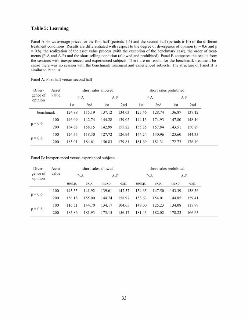
Table 5 addresses the learning hypothesis. Since the three price measures yield very

similar conclusions we restrict the presentation to the equally weighted mean price. In Panel A

of Table 5 we report separate results for the first half (periods 1-5) and the second half (periods

6-10) of each treatment condition. The results do not support the hypothesis that the impact of

short selling restrictions on prices decreases with experience. Both in the first half and in the

second half prices are higher when short sales are restricted in 6 out of a total of 10 cases. The

most severe overvaluation is observed in the second half of the PA60 treatment when the true

asset value is low. The average price is 174.93 when short sales are prohibited and 142.74

when they are allowed. Panel B of Table 5 compares the results from the sessions with inexpe-

rienced and experienced subjects. Again, there is not much evidence that the impact of short

selling restrictions on prices decreases with experience. For both groups, prices are higher

12 In Panel C there is a third exception in the "all" column for p=0.8 and a high asset value.

22

when short selling is prohibited in six out of eight cases. The results in Table 5 thus suggest

that the (weak) support for the overvaluation hypothesis documented earlier is not attributable

to inexperienced subjects.

So far we have solely compared prices obtained under different treatment conditions.

To obtain a more complete picture of the relation between short sale constraints and asset

valuation we augment these univariate statistics with a pooled regression model. The depend-

ent variable is the (equally weighted) average price13 in each of 20 periods14 of the 18 sessions.

The price is likely to depend on the treatment and on the realization of the asset value process.

For example, when p = 0.8 subjects have more precise information as compared to the case

where p = 0.6. We should thus expect higher prices in the p = 0.8 treatments when the true

value is high and lower prices when the true value is low. To capture these effects we include

dummy variables for each treatment (except AP0 which is the base case) and interaction terms,

defined as the product of the treatment dummies and a dummy variable that equals one when

the realized asset value is high.

Besides these control variables we include a dummy variable that equals one when

short selling is prohibited (model 1). The overvaluation hypothesis predicts a positive coeffi-

cient. In an additional model (model 2) we further add two interaction terms that interact the

no-short-sales dummy with two dummy variables taking on the value one when p = 0.6 and p =

0.8, respectively. The coefficients on these interaction terms measure whether the overvalua-

13 Using the digitally weighted average price or the bid-ask midpoint instead yields similar conclusions. 14 In period 14 of one session (PA60E) no transaction took place. The total number of observations in the regres-sion is thus 359.

23

tion is more pronounced when the degree of divergence of opinion increases. The overvalua-

tion hypothesis predicts a positive coefficient.

The results are presented in Table 6. The adjusted R2 for both models is 0.5. The con-

trol and treatment variables thus explain about half of the variation in prices. Many of the

treatment dummies and the interactions of the treatment dummies with the asset value dummy

are significant, and most of the coefficients have the expected sign. Most importantly, prices

are significantly higher when short sales are prohibited. The coefficient on the no-short-sales

dummy is 4.51 (t-statistic 2.28) in model one and 4.14 (t-statistic 3.03) in model 2. These re-

sults are consistent with Hypothesis 3.

The coefficients on the additional interaction terms in model 2 are far from being sig-

nificant. Thus, contrary to Hypothesis 4 (but consistent with our previous results), overvalua-

tion does not increase in the degree of divergence of opinion.

6 Summary and conclusion

The overvaluation hypothesis first put forward by Miller (1977) predicts that assets will

be overvalued when (a) short sale constraints and (b) differences of opinion exist. Numerous

empirical studies have been conducted in order to test the overvaluation hypothesis. The results

of these studies are not fully conclusive, partially due to measurement problems. Neither the

existence (and degree, respectively) of short selling constraints nor the degree of divergence of

opinion and the true value of a stock is observable, directly.

To avoid the shortcomings of previous empirical studies, we use an experimental ap-

proach. In the laboratory, trading of assets can be observed under ceteris paribus conditions

with and without short selling constraints. We can thus examine the impact of short selling

24

constraints on valuation. Our design further allows varying the degree of divergence of opinion

across markets.

The results are only partially supportive of the overvaluation hypothesis. We find evi-

dence of higher asset values in the presence of short sale constraints. We do not find, however,

that overvaluation is increasing in the degree of divergence of opinion. We further document

that trading volume is lower under short sale constraints, and that the overvaluation does not

decrease when subjects are experienced.

25

References

Ackert, L., N. Charupat, B. Church and R. Deaves (2002): Bubbles in Experimental Asset

Markets: Irrational Exuberance no More. Federal Reserve Bank of Atlanta Working

Paper 2002-24, December.

Aitken, M., A. Frino, M. McCorry and P. Swan (1998): Short Sales are Almost Instantaneously

Bad News: Evidence from the Australian Stock Exchange. Journal of Finance 53, 2205-

2223.

Asquith, P. and L. Meulbroek (1996): An Empirical Investigation of Short Interest. Working

Paper, Harvard University.

Asquith, Paul, P. Pathak and J. Ritter (2005): Short Interest, Institutional Ownership and Stock

Returns. Journal of Financial Economics 78, 243-276.

Boehme, R., B. Danielsen and S. Sorescu (2005): Short Sale Constraints, Difference of Opin-

ion, and Overvaluation. Forthcoming in: Journal of Financial and Quantitative Analysis

Brent, A., D. Morse and E.K. Stice (1990): Short Interest: Explanations and Tests. Journal of

Financial and Quantitative Analysis 25, 273-289.

Bris, A., W. Goetzmann and N. Zhu (2004): Efficiency and the Bear: Short Sales and Markets

around the World. Yale ICF Working Paper 02-45, September.

Chang, E. and Y. Yu (2004): Short-Sales Constraints and Price Discovery: Evidence from the

Hong Kong Market. Working Paper, University of Hong Kong, March.

Charoenrook, A. and H. Daouk (2005): A Study of Market-Wide Short-Selling Restrictions.

Working Paper, January.

26

Cohen, L., K. Diether and Ch. Malloy (2005): Supply and Demand Shifts in the Shorting Mar-

ket. Working Paper, May.

D'Avolio, G. (2002): The Market for Borrowing Stock. Journal of Financial Economics 66,

271-306.

Danielsen, B.R. and S.M. Sorescu (2001): Why Do Option Introductions Depress Stock

Prices? A Study of Diminishing Short-Sale Constraints. Journal of Financial and Quan-

titative Analysis 36, 451-484.

Dechow, P.M., A.P. Hutton, L. Meulbroek and R.G. Sloan (2001): Short-Sellers, Fundamental

Analysis and Stock Returns. Journal of Financial Economics 61, 77-106.

Desai, H., K. Ramesh, S.R. Thiagarajan and B.V. Balachandran (2002): An Investigation of the

Informational Role of Short Interest in the Nasdaq Market. Journal of Finance 57,

2263-2287.

Diamond, D. and R. Verrecchia (1987): Constraints on Short-Selling and Asset Price Adjust-

ment to Private Information. Journal of Financial Economics 18, 277-311.

Diether, K., K.-H. Lee and I. Werner (2005): Can Short Sellers Predict Returns? Daily Evi-

dence. Working Paper, Ohio State University, July.

Diether, K.B., C.J. Malloy and A. Scherbina (2002): Differences of Opinion and the Cross-

Section of Stock Returns. Journal of Finance 57, 2113-2141.

Duffie, D., N. Garleanu and L.H. Pedersen (2002): Securities Lending, Shorting and Pricing.

Journal of Financial Economics 66, 307-339.

Figlewski, S. and G.P. Webb (1993): Options, Short Sales, and Market Completeness. Journal

of Finance 48, 761-777.

27

Fischbacher, U. (1999): z-Tree: A Toolbox for Readymade Economic Experiments. Working

Paper, University of Zurich.

Francis, J, M. Venkatachalam and Y. Zhang (2005): Do Short Sellers Convey Information

About Changes in Fundamentals or Risk? Working Paper, Duke University, September.

Gopalan, M. (2003): Short Constraints, Difference of Opinion and Stock Returns. Working

Paper, Duke University.

Greiner, B. (2004): The online recruitment system ORSEE 2.0 – a guide for the organization of

experiments in economics, Working Paper Series in Economics 10, University of Co-

logne.

Haruvy, E. and Ch. Noussair (2005): The Effect of Short Selling on Bubbles and Crashes in

Experimental Spot Asset Markets. Forthcoming in: Journal of Finance.

Hong, H. and J. Stein (2003): Differences of Opinion, Short Sales Constraints and Market

Crashes. Review of Financial Studies 16, 487-525.

Jiang, D. (2005): Overconfidence, Short-Sale Constraints, and Stock Valuation. Working Pa-

per, Ohio State University, September.

Johnson, T. (2004): Forecast Dispersion and the Cross Section of Expected Returns. Journal of

Finance 59, 1957-1978.

Jones, C.M. and O.A. Lamont (2002): Short Sale Constraints and Stock Returns. Journal of

Financial Economics 66, 207-239.

King, R., V. Smith, A. Williams, and M. Van Boening (1993): The Robustness of Bubbles and

Crashes in Experimental Stock Markets. In: I. Prigogine, R. Day, and P. Chen (Eds.):

Nonlinear Dynamics and Evolutionary Economics, Oxford: Oxford University Press.

28

Mayhew, S. and V. Mihov (2004): Short Sale Constraints, Overvaluation and the Introduction

of Options. Working Paper, SEC and Texas Christian University, December.

Miller, E. (1977): Risk, Uncertainty, and Divergence of Opinion. Journal of Finance 32, 1151-

1168.

Nagel, S. (2005): Short Sales, Institutional Investors and the Cross-Section of Stock Returns.

Journal of Financial Economics 78, 277-309.

Ofek, E., M. Richardson and R. Whitelaw (2004): Limited Arbitrage and Short Sale Restric-

tions: Evidence from the Options Market. Journal of Financial Economics 74, 305-342.

Reed, A. (2003): Costly Short-Selling and Stock Price Adjustment to Earnings Announce-

ments. Working Paper, University of North Carolina, June.

Scheinkman, J. and X. Wei (2003): Overconfidence and Speculative Bubbles. Journal of Po-

litical Economy 111, 1183-1219.

Smith, V., G. Suchanek, and A. Williams (1988): Bubbles, Crashes, and Endogenous Expecta-

tions in Experimental Spot Asset Markets. Econometrica 56, 1119-1151.

29

Table 1: Parameter choice

The table shows the parameters used in the individual experimental treatments. It further shows the expected value of the asset conditional on the signal and the expected number of traders with a correct and an incorrect signal. The full information benchmark is the expected value of the asset conditional on all 10 signals and under the assumption that the numbers of correct and incorrect signals are equal to their expected values. The last line shows the measure of divergence of opinion, θ. p = 0 (benchmark) p = 0.6 p = 0.8 asset value asset value asset value high low high low high low

asset value 200 100 200 100 200 100

cond. expectation of trader with signal h na na 160 160 180 180

expected number of traders with signal h na na 6 4 8 2

cond. expectation of trader with signal l na na 140 140 120 120

expected number of traders with signal l na na 4 6 2 8

full information bench-mark 150 150 169.23 130.77 199.98 100.02

measure of divergence of opinion (θ) 0 0.0096 0.0576

30

Table 2: Treatment summary

The table describes the treatments and shows the number of sessions that were conducted with each treatment condition. sequence of treatments Signal precision short selling prohibited - short sell-

ing allowed (PA) short selling allowed - short selling

prohibited (AP)

no signals (benchmark case) PA0 - session 1 AP0 session 10

p = 0.6 PA60 - sessions 2-4 PA60E - session 5

AP60 sessions 11-13 AP60E - session 14

p = 0.8 PA80 - sessions 6-8 PA80E - session 9

AP80 sessions 15-17 AP80E - session 18

31

Table 3: Trading volume

The table shows the mean and the median trading volume per period for the different treatment conditions. Col-umns 5 and 8 report the t-statistic and the z-statistic for a test of the null hypothesis of equal means and medians, respectively. The last line shows results pooled over all treatment conditions.

mean volume per period median volume per period Diver-gence of opinion

Order of treatments short sales

allowed short sales prohibited

t-statistic (p-value)

short sales allowed

short sales prohibited

z-statistic (p-value)

P-A 27.10 33.30 1.19 26.50 33.50 1.14 Bench-mark A-P 10.60 8.00 2.29 11.00 8.00 1.99

P-A 13.73 14.78 0.44 13.50 9.50 0.80 p = 0.6

A-P 27.85 13.25 5.03 26.50 12.00 4.88

P-A 14.63 11.80 1.75 13.50 12.00 1.22 p = 0.8

A-P 23.60 9.63 4.24 16.50 8.00 3.97

pooled 19.83 13.28 4.89 15.50 10.50 5.04

32

Table 4: Price Levels

The table shows the mean price per period for the different treatment conditions. We report separate results for periods with low and high asset values, respectively (no such distinction is made in the benchmark treatment because there traders did not receive signals about the asset value). Columns 3-5 (6-8) report the prices for those periods where short sales were allowed (prohibited). We provide separate results for those sessions were the order of treatments was P-A and A-P, respectively, as well as aggregated results. Columns 9-11 show the t-statistics for the null hypothesis of equal means. The t-statistic in column 9 (10; 11) relate to a comparison of the prices in columns 3 and 6 (4 and 7; 5 and 8). Panel A: Mean price, equally weighted

short sales allowed short sales prohibited t-statistic Diver-gence of opinion

Asset value

P-A A-P all P-A A-P all P-A A-P all

Benchmark 120.04 135.88 127.96 128.10 136.99 132.55 3.40 0.95 1.87

100 144.11 141.41 142.76 153.75 147.95 150.33 1.71 1.52 2.20 p = 0.6

200 156.11 148.69 152.30 157.09 147.42 153.08 0.21 0.23 0.21

100 122.77 127.36 124.70 138.60 130.51 134.32 1.77 0.31 1.44 p = 0.8

200 184.79 168.74 175.95 181.50 175.07 178.42 0.63 0.96 0.56 Panel B: Mean price, digitally weighted

short sales allowed short sales prohibited t-statistic Diver-gence of opinion

Asset value

P-A A-P all P-A A-P all P-A A-P all

Benchmark 119.84 136.18 128.01 127.94 136.91 132.43 3.14 0.60 1.73

100 143.69 139.33 141.51 154.39 148.31 150.80 1.79 2.00 2.55 p = 0.6

200 155.38 148.77 151.98 157.01 147.79 153.19 0.33 0.16 0.31

100 120.16 125.89 122.57 137.52 129.89 133.48 1.78 0.38 1.55 p = 0.8

200 187.30 169.91 177.72 184.78 176.23 180.69 0.49 0.94 0.67 Panel A: Bid-ask midpoint

short sales allowed short sales prohibited t-statistic Diver-gence of opinion

Asset value

P-A A-P all P-A A-P all P-A A-P all

Benchmark 118.71 135.46 127.08 132.96 137.35 135.16 6.37 1.40 3.42

100 141.92 144.13 143.03 153.22 147.88 150.07 2.23 1.12 2.40 p = 0.6

200 154.70 149.48 152.09 156.40 149.16 153.40 0.38 0.08 0.43

100 118.97 128.54 122.98 134.50 134.57 134.54 2.16 0.81 2.25 p = 0.8

200 179.34 167.16 172.49 173.05 169.63 171.41 1.29 0.59 0.33

33

Table 5: Learning

Panel A shows average prices for the first half (periods 1-5) and the second half (periods 6-10) of the different treatment conditions. Results are differentiated with respect to the degree of divergence of opinion (p = 0.6 and p = 0.8), the realization of the asset value process (with the exception of the benchmark case), the order of treat-ments (P-A and A-P) and the short selling condition (allowed and prohibited). Panel B compares the results from the sessions with inexperienced and experienced subjects. There are no results for the benchmark treatment be-cause there was no session with the benchmark treatment and experienced subjects. The structure of Panel B is similar to Panel A. Panel A: First half versus second half

short sales allowed short sales prohibited

P-A A-P P-A A-P

Diver-gence of opinion

Asset value

1st 2nd 1st 2nd 1st 2nd 1st 2nd

benchmark 124.88 115.19 137.12 134.63 127.46 128.74 136.87 137.12

100 146.09 142.74 144.28 139.02 144.13 174.93 147.80 148.10 p = 0.6

200 154.68 158.15 142.99 155.82 155.85 157.84 143.51 150.89

100 126.35 118.30 127.72 126.94 146.24 130.96 123.60 144.33 p = 0.8

200 185.01 184.61 156.83 179.81 181.69 181.31 172.73 176.40 Panel B: Inexperienced versus experienced subjects

short sales allowed short sales prohibited

P-A A-P P-A A-P

Diver-gence of opinion

Asset value

inexp. exp. inexp. exp. inexp. exp. inexp. exp.

100 145.35 141.92 139.61 147.57 154.65 147.50 143.39 158.36 p = 0.6

200 156.18 155.00 144.74 158.97 158.63 154.01 144.85 159.41

100 116.51 144.70 134.17 104.65 149.00 125.23 134.08 117.99 p = 0.8

200 185.86 181.93 173.15 156.17 181.43 182.02 178.23 166.63

34

Table 6: Regression results

The table shows the results of OLS regressions. The dependent variable is the average price of each period. We include control variables for the different treatment conditions and interactions between these control variables and a dummy that is equal to 1 whenever the asset value is high. In model 1 we include a dummy variable that equals 1 when short selling is prohibited. In model 2 we further include interactions between the short selling dummy and dummy variables that equal 1 in those sessions where p = 0.6 and p = 0.8 (denoted div 60 and div 80), respectively. The number of observations is 359 (18 sessions, each with 20 periods; in one period no transac-tion took place). t-values are based on heteroscedasticity-consistent standard errors. Model 1 Model2 coefficient t-value coefficient t-value constant 134.84 70.90 135.09 79.79 AP60 4.41 1.63 4.30 1.44 AP80 -3.36 -0.54 -3.83 -0.58 AP60E 16.39 3.77 16.31 3.40 AP80E -25.15 -7.33 -25.61 -6.31 PA0 -10.76 -5.67 -10.80 -5.75 PA60 12.90 3.43 12.80 3.30 PA80 -7.39 -1.49 -7.78 -1.45 PA60E 7.29 1.60 7.10 1.53 PA80E -5.41 -0.54 -5.90 -0.54 Value200 -1.21 -0.76 -1.32 -0.88 AP60*Value200 4.42 1.07 4.54 1.11 AP80*Value200 43.12 5.79 43.29 5.80 AP60E*Value200 7.42 1.07 7.47 1.07 AP80E*Value200 50.43 8.53 50.58 8.71 PA0*Value200 -3.83 -1.42 -3.76 -1.41 PA60*Value200 8.62 1.85 8.73 1.90 PA80*Value200 54.54 9.76 54.58 9.81 PA60E*Value200 9.18 1.31 9.50 1.37 PA80E*Value200 52.23 3.76 52.46 3.75 no short sales 4.51 2.28 4.14 3.03 no short sales*div60

0.07 0.03

no short sales*div80

0.75 0.19

adj. R2 0.50 0.50