Shocks in unmagnetized plasma with a shear

flow: Stability and magnetic field generation

Mark Eric Dieckmann, Alexander Bock, Hamad Ahmed, Domenico Doria, Gianluca Sarri,

Anders Ynnerman and Marco Borghesi

Linköping University Post Print

N.B.: When citing this work, cite the original article.

Original Publication:

Mark Eric Dieckmann, Alexander Bock, Hamad Ahmed, Domenico Doria, Gianluca Sarri,

Anders Ynnerman and Marco Borghesi, Shocks in unmagnetized plasma with a shear flow:

Stability and magnetic field generation, 2015, Physics of Plasmas, (22), 7, 1-9.

http://dx.doi.org/10.1063/1.4926525

Copyright: American Institute of Physics (AIP)

http://www.aip.org/

Postprint available at: Linköping University Electronic Press

http://urn.kb.se/resolve?urn=urn:nbn:se:liu:diva-120108

Shocks in unmagnetized plasma with a shear flow: Stability and magnetic fieldgenerationM. E. Dieckmann, A. Bock, H. Ahmed, D. Doria, G. Sarri, A. Ynnerman, and M. Borghesi Citation: Physics of Plasmas 22, 072104 (2015); doi: 10.1063/1.4926525 View online: http://dx.doi.org/10.1063/1.4926525 View Table of Contents: http://scitation.aip.org/content/aip/journal/pop/22/7?ver=pdfcov Published by the AIP Publishing Articles you may be interested in Ion acoustic shocks in magneto rotating Lorentzian plasmas Phys. Plasmas 21, 122120 (2014); 10.1063/1.4905060 Convective radial energy flux due to resonant magnetic perturbations and magnetic curvature at the tokamakplasma edge Phys. Plasmas 21, 082502 (2014); 10.1063/1.4891437 Modification of the formation of high-Mach number electrostatic shock-like structures by the ion acousticinstability Phys. Plasmas 20, 102112 (2013); 10.1063/1.4825339 Laboratory and computer simulations of super-Alfvénic shocks in a weakly ionized medium Phys. Plasmas 10, 605 (2003); 10.1063/1.1539473 Generation of magnetic field and electrostatic shock wave driven by counterstreaming pair plasmas Phys. Plasmas 10, 392 (2003); 10.1063/1.1540095

This article is copyrighted as indicated in the article. Reuse of AIP content is subject to the terms at: http://scitation.aip.org/termsconditions. Downloaded to IP:

130.236.83.116 On: Tue, 08 Sep 2015 12:17:16

Shocks in unmagnetized plasma with a shear flow: Stability and magneticfield generation

M. E. Dieckmann,1 A. Bock,1 H. Ahmed,2 D. Doria,2 G. Sarri,2 A. Ynnerman,1

and M. Borghesi21Department of Science and Technology, Link€oping University, SE-60174 Norrk€oping, Sweden2Centre for Plasma Physics (CPP), Queen’s University Belfast, BT7 1NN, United Kingdom

(Received 18 April 2015; accepted 22 June 2015; published online 8 July 2015)

A pair of curved shocks in a collisionless plasma is examined with a two-dimensional

particle-in-cell simulation. The shocks are created by the collision of two electron-ion clouds at a

speed that exceeds everywhere the threshold speed for shock formation. A variation of the collision

speed along the initially planar collision boundary, which is comparable to the ion acoustic speed,

yields a curvature of the shock that increases with time. The spatially varying Mach number of the

shocks results in a variation of the downstream density in the direction along the shock boundary.

This variation is eventually equilibrated by the thermal diffusion of ions. The pair of shocks is

stable for tens of inverse ion plasma frequencies. The angle between the mean flow velocity vector

of the inflowing upstream plasma and the shock’s electrostatic field increases steadily during this

time. The disalignment of both vectors gives rise to a rotational electron flow, which yields the

growth of magnetic field patches that are coherent over tens of electron skin depths. VC 2015AIP Publishing LLC. [http://dx.doi.org/10.1063/1.4926525]

I. INTRODUCTION

The collision of an ionized blast shell with an ambient

plasma triggers the formation of shocks if the collision speed

exceeds a threshold value. The critical speed depends on the

plasma wave mode that is mediating the shock and on the

importance of Coulomb collisions between particles. If the

mean frequency, with which the plasma particles collide, is

well below all resonance frequencies of the plasma, then the

effects of binary collisions are negligible and the shocks are

mediated by electrostatic and electromagnetic fields.

The plasma processes that sustain a collisionless shock

and the structure of the associated electromagnetic fields

vary strongly between the different plasma regimes. Solar

system shocks, like the Earth’s bow shock,1,2 are immersed

in a plasma that is carrying a relatively strong magnetic field

and they connect two plasmas that collide at a non-

relativistic speed. Such shocks are usually mediated by mag-

netosonic waves. The collision speed between a supernova

blast shell and the interstellar medium (ISM) at a late evolu-

tion phase is similar to the collision speed between the solar

wind and the Earth’s bow shock. The amplitude of the mag-

netic field in the ISM, into which a supernova remnant (SNR)

shock expands, is weaker by an order of magnitude than that

in the solar wind plasma at the Earth’s orbit. Magnetosonic

waves, which have a low field amplitude, may not be able to

sustain permanently the shock because other instabilities de-

velop faster and on a smaller spatial scale. Simulations have

shown that drift instabilities and electrostatic turbulence can

in some cases suppress the growth of a magnetosonic wave.3

As we go to higher flow speeds, the plasma shocks become

magnetized by filamentation instabilities.4–7

We consider here shocks, which develop in an initially

unmagnetized and collisionless plasma. Such shocks are

frequently observed in the laboratory8–13 and they might be

representative for SNR shocks in their late evolution phase.

An electrostatic shock in its most basic form is characterized

by a potential difference, which is sustained self-consistently

by the plasma. The shock connects the downstream region

and an upstream region ahead of the shock. Electrons stream

from the denser downstream region into the upstream region

and create a charge imbalance between both regions. The

denser downstream plasma goes on a positive potential rela-

tive to the upstream plasma.

The upstream plasma streams towards the shock at a

speed, which exceeds the ion acoustic speed. The upstream

ions are slowed down and compressed by the potential jump

as they cross the shock. The potential jump reflects some of

the incoming upstream ions, which then move back

upstream. The remainder of the incoming ions enters the

downstream region, which expands due to the accumulation

of the inflowing ions. The shock is thus not stationary in the

downstream frame of reference and moves upstream.

An electrostatic shock is an ion phase space structure,

which consists of inflowing upstream ions, reflected ions and

ions that overcame the positive potential and accumulated

downstream of the shock. The electrostatic field, which

mediates the shock, will also accelerate some of the down-

stream ions into the upstream direction and act as a double

layer. Many shocks in unmagnetized plasma are a combina-

tion of a double layer and of an electrostatic shock. Such

hybrid structures14 are characterized by a unipolar electric

field. In what follows we shall refer to these hybrid structures

as plasma shocks to distinguish them from pure electrostatic

shocks.

The incoming upstream ions, which have been reflected

by the electrostatic shock, and the downstream ions, which

have been accelerated upstream by the double layer, form a

1070-664X/2015/22(7)/072104/9/$30.00 VC 2015 AIP Publishing LLC22, 072104-1

PHYSICS OF PLASMAS 22, 072104 (2015)

This article is copyrighted as indicated in the article. Reuse of AIP content is subject to the terms at: http://scitation.aip.org/termsconditions. Downloaded to IP:

130.236.83.116 On: Tue, 08 Sep 2015 12:17:16

beam that outruns the plasma shock. We shall refer to this

beam as the shock-reflected ion beam. The number density

of this beam can be a significant fraction of that of the

incoming upstream ions, which implies that the ion number

density ahead of the plasma shock is well above that in the

far upstream region. In what follows, we refer to this region

as the foreshock.

The counterstreaming nonrelativistic and unmagnetized

ion beams drive the electrostatic ion acoustic instability in

the foreshock.15,16 The speed of the shock-reflected ions in

the upstream frame of reference exceeds the ion acoustic

speed. The ion acoustic instability can, however, only be

destabilized if the beam velocity component along the wave

vector is subsonic. The wave vectors of the unstable waves

can thus not be parallel to the plasma flow velocity vector.

Oblique electrostatic waves grow and the obliquity angle is

such that the beam velocity component along the wave vec-

tor is comparable to the ion acoustic speed.17 Obliquely

propagating ion acoustic waves grow in the foreshock region

and modulate the incoming upstream ions. The plasma shock

is either transformed into a shock with a broad transition

layer3 or it is destroyed by the inflowing turbulent plasma.16

Previous simulation studies have addressed the evolu-

tion of (quasi-)planar plasma shocks. The planarity has been

enforced in the particle-in-cell (PIC) simulations by resolv-

ing only one spatial direction or by choosing initial condi-

tions that are uniform along one direction. However, in

particular, the plasma shocks in laboratory experiments are

often nonplanar. This motivates our study of the formation

and evolution of curved shocks with a PIC simulation.

The shock curvature is introduced in our simulation

through the following setup. The two electron-ion clouds

collide at a boundary, which is orthogonal to the spatially

uniform collision direction at the simulation’s start. The

mean speed of the plasma along the collision direction varies

as a function of the orthogonal direction and this velocity

shear gives rise to a shock front that becomes increasingly

curved in time. The amplitude of the velocity change is com-

parable to the ion acoustic speed.

We find that the shock formation and its stability are not

affected by this large velocity shear. The life-time of the

plasma shocks is of the order of tens of inverse ion plasma

frequencies. The shock transition layer is transformed after

this time by the onset of ion acoustic turbulence in the fore-

shock. The transition from a sharp electron skin depth-scale

structure into a broad transition layer is also observed for

planar shocks. The key difference between the structure of

the curved shock and a planar shock is tied to the disalign-

ment of the electric field with the flow velocity vector of the

incoming upstream plasma. The disalignment gives rise to a

rotational component of the electron flow, which yields the

growth of magnetic field patches. These patches are coherent

over tens of electron skin depths and their size is limited by

the simulation box dimension. Their amplitude yields a ratio

of the electron plasma frequency to the cyclotron frequency

of about 100.

Our paper is structured as follows. Section II discusses

the PIC code and the initial conditions we use. Section III

examines the formation and the evolution of the pair of elec-

trostatic shocks. Section IV summarizes our findings.

II. INITIAL CONDITIONS AND THE PIC METHOD

PIC simulation codes18 solve the Vlasov-Maxwell sys-

tem of equations via the method of characteristics.19 The

electromagnetic fields are evolved in time via Ampere’s law

and Faraday’s law

l0�0

@E

@t¼ r� B� l0J; (1)

@B

@t¼ �r� E: (2)

Most codes fullfill the equations r � E ¼ q=�0 and r � B ¼ 0

either as constraints or via correction steps. The plasma is

approximated by an ensemble of computational particles

(CPs), which correspond to volume elements of the phase

space density distribution. The charge-to-mass ratio of the

CPs equals that of the plasma particles they represent. Their

momentum and position are updated with the relativistic

Lorentz force equation

dpj

dt¼ qi E xjð Þ þ vj � B xjð Þ

� �: (3)

The CP with the index j of the species i with the position xj

and the relativistic momentum pj ¼ miCjvj has the charge qi

and the mass mi. Its position is updated by dxj=dt ¼ vj. The

CPs and the electromagnetic fields Eðx; tÞ and Bðx; tÞ are

connected as follows. The fields are interpolated to the parti-

cle position and update its momentum in time. The current

density contribution of each CP is interpolated to the grid.

The summation over all current density contributions yields

the macroscopic current density Jðx; tÞ, which updates the

electromagnetic fields via Ampere’s law.

A pair of shocks is generated in the simulation by the

collision of two spatially uniform plasma clouds of equal

density. Each cloud consists of electrons with the charge–e(e: elementary charge), the mass me, the number density n0,

and the temperature Te¼ 1 keV. We model Deuterium ions

with the number density n0, the mass mD, and the tempera-

ture TD¼ 200 eV. We motivate our choice for the initial con-

ditions as follows.

The collision of two plasma clouds in laboratory- or

astrophysical settings usually involves two plasmas with

densities that differ by orders of magnitude. The blast shell,

which is ejected during a supernova, is composed of stellar

material. Its density is thus initially much higher than that of

the ambient plasma, which is the stellar wind the star ema-

nated prior to the supernova. A laser-generated blast shell is

also much denser than the ambient medium, which is the

residual gas that has been ionized by secondary x-ray radia-

tion from the target.

The blast shells are practically unaffected by the ambi-

ent medium during their initial expansion phase and they

expand in the form of rarefaction waves. The front of the

blast shell becomes faster and thinner in time. Once the

expansion speed of the blast shell becomes supersonic and

072104-2 Dieckmann et al. Phys. Plasmas 22, 072104 (2015)

This article is copyrighted as indicated in the article. Reuse of AIP content is subject to the terms at: http://scitation.aip.org/termsconditions. Downloaded to IP:

130.236.83.116 On: Tue, 08 Sep 2015 12:17:16

once the ram pressure of the expanding blast shell becomes

comparable to the thermal pressure of the ambient medium,

the front can be confined and shocks form. Experimental

observations13 and PIC simulations20 suggest that shocks

form when the densities of the colliding clouds become com-

parable. Selecting equal densities for both colliding plasma

clouds should thus be a valid initial condition.

The electron and ion temperatures we use are typical for

plasmas, which are created when an ultrashort laser pulse

ablates a solid target and if time scales are considered, which

are short compared to the time it takes to establish a thermal

equilibrium via collisions between electrons and ions. The

temperature of the electrons in the ambient plasma, which

has been ionized by secondary x-ray emissions from the

laser-ablated target, is comparable to 1 keV. The tempera-

tures of the ions of the ambient medium and of the blast shell

are usually well below that of the electrons.21

Deuterium ions have the same charge-to-mass ratio as

the fully ionized light atoms, which we usually encounter in

laser-plasma experiments, and they have the largest thermal

velocity spread for a given temperature. Hence they will pro-

vide the strongest ion Landau damping. If we observe the

growth of ion acoustic waves for counter-streaming beams

of Deuterium, then the same will be true for equally hot plas-

mas, which consist of heavier ions with the same charge-to-

mass ratio as Deuterium.

The plasma frequencies of the electrons and of the ions

are xp;e ¼ ðn0e2=�0meÞ1=2and xp;i ¼ ðme=mDÞ1=2xp;e,

respectively. The ion acoustic speed in this plasma is cs ¼ðcckBðTe þ TDÞ=mDÞ1=2

assuming that the adiabatic constant

cc ¼ 5=3 is the same for both species. The ion acoustic speed

is cs ¼ 3:1� 105 m/s.

The simulation domain has the dimensions

Lx � Ly ¼ 176ks � 26:2ks, where ks ¼ c=xp;e is the electron

skin depth. The boundary conditions are periodic along y and

open along x. Choosing periodic boundaries along y implies

that our simulation evolves in time a periodic chain of blast

shells rather than a solitary one. The simulation domain is

split up into two equal parts along x. The blast shell occupies

the interval �Lx=2 � x � 0 and �Ly=2 < y � Ly=2. The

second cloud, which we refer to as the ambient plasma, occu-

pies the interval 0 < x < Lx=2 and �Ly=2 < y � Ly=2.

The initial mean speeds of the electrons and ions of the

ambient plasma vanish. The mean speed of the blast shell’s

electrons equals that of the ions and is denoted here as

v ¼ ð�vx; 0; 0Þ. The value of �vx varies piecewise linearly

along the y-axis. The largest value of �vx ¼ 1:15� 106 m/s

or 3:7cs is reached at the position y¼ 0. The speed

decreases linearly in both y-directions. It reaches its

minimum of 8:7� 105 m/s or 2:8cs at the boundaries at

y ¼ �Ly=2 and y ¼ Ly=2.

The simulation box is resolved by 4000 grid cells along

the x-direction and by 600 cells along the y-direction. The

quadratic side length of each cell is Dx ¼ 0:044ks. Each

plasma species is resolved by 200 CPs per cell. We evolve

the system for Tsimxp;i ¼ 153 using 3:2� 105 time steps Dt.

In what follows, we normalize time to 1=xp;i, space to ks and

speed to the electron thermal speed vth;e ¼ ðkBTe=meÞ1=2.

The electric field is normalized to mexp;ec=e and the mag-

netic one to mexp;e=e.

III. THE SIMULATION RESULTS

In what follows, we shall present and discuss the spatial

distributions of the ion density, of the amplitude of the flow-

aligned electric field component Exðx; yÞ and the out-of-plane

magnetic field distribution Bzðx; yÞ at the times t¼ 6, 13.8,

19.4, 33.8, 70, and 153.

Figure 1 shows the ion density, the electric Ex compo-

nent and the magnetic Bz component close to the initial con-

tact boundary x¼ 0 at several times. A band with an

increased ion density is visible in Fig. 1(a). The ions of both

clouds interpenetrate and their cumulative density exceeds

n0. The peak density of the ions is reached at x � 0:7 and it

exceeds 2n0 for all values of y. This ion cloud overlap layer

is broadest at y � 0. At this time the ions of both clouds

move independently and the width of the layer is propor-

tional to the speed at which the clouds collide. The ion den-

sity is not constant close to its maximum value in Fig. 1(d).

Hence, a downstream region, which is characterized by a

spatially uniform plasma distribution along x that separates

the forward and reverse shocks, has not formed at this time.

A strong bipolar electric field pulse is visible in Fig.

1(b). It is sustained by the space charge, which results from

the electrons that escaped from the ion cloud overlap layer.

The polarity of the electric field is such that the ion cloud

overlap layer is on a positive potential relative to the ambi-

ent- and blast shell plasmas. The slow-down of the inflowing

ions by this potential is responsible for the increase of the

ion density beyond 2n0.

Figure 1(c) reveals magnetic oscillations within the ion

cloud overlap layer. The strongest oscillations are located at

y � 0 and x � 0:7, where the plasma collides at the highest

speed. The growth of Bz within the ion cloud overlap layer

can be attributed partially to the instability observed in

Ref. 22 for shocks and in Refs. 23 and 24 for rarefaction

waves. The electrons are accelerated along the electric field

of the ion cloud overlap layer. The resulting directional ani-

sotropy in the velocity distribution triggers the Weibel

instability.25,26

The Weibel instability in the form discussed in Ref. 26

can, however, not explain why the magnetic field oscillations

peak at y � 0 and x � 0:5. We attribute this to the geometric

effect that is outlined in Fig. 2.

We consider first the boundaries between the overlap

layer and the upstream plasma that have a constant slope.

Electrons that stream into the overlap layer are accelerated

by the ambipolar electric field that ensheaths the overlap

layer. The field is aligned with the boundary normal. The

electrons are accelerated and the ions are decelerated when

they enter the overlap layer, while their lateral velocity com-

ponents remain unchanged. The velocity vectors of the

inflowing electrons and ions are thus rotated into opposite

directions. Their current contributions do no longer cancel

each other out and a net current develops within the overlap

layer.

072104-3 Dieckmann et al. Phys. Plasmas 22, 072104 (2015)

This article is copyrighted as indicated in the article. Reuse of AIP content is subject to the terms at: http://scitation.aip.org/termsconditions. Downloaded to IP:

130.236.83.116 On: Tue, 08 Sep 2015 12:17:16

An even stronger net current develops close to the cusps

due to the changing direction of the normal. Electrons that

cross the overlap layer at a concave cusp are scattered.

Electrons that cross it at a convex cusp are focused. The elec-

tron current is no longer balanced along the vertical direction

in the center of Fig. 2. A net current flows from the concave

to the convex cusp of the overlap layer and a magnetic field

will grow, which is at least initially confined to the overlap

layer. The growing spatially localized magnetic field will

induce a ring current within the overlap layer. The direction

of the magnetic field in Fig. 2 matches that in the simulation

if we take into account that the z-axis points into the plot’s

plane in Fig. 1(c).

Magnetic field oscillations are present on both sides of

the ion cloud overlap layer in Fig. 1(c). Their wavelength is

2p=Ly along y. This modulation extends up to the boundary

at �Lx=2 and it does not oscillate along the x-direction (not

shown). Such an oscillation cannot be driven by an electron

current that emanates from the overlap layer. Electrons that

move at the thermal speed can only traverse the distance

FIG. 1. The ion density distributions expressed in units of n0 are shown in the first column (from left to right). The distributions of Exðx; yÞ are shown in the

second column. The electric amplitudes have been multiplied by a factor 100. The third column shows the distributions of Bzðx; yÞ and the right column shows

slices of the ion density distributions along y¼ 0 (dashed blue) and along y¼ 13.1 (black). The upper row corresponds to the time t¼ 6, the second row to

t¼ 13.8, the third one to t¼ 19.4 and the bottom row to t¼ 33.8.

FIG. 2. The field and flow diagram within the overlap layer of both plasma

clouds. The normals of the boundary between the overlap layer and the

upstream plasma are denoted by N and are parallel to the vector of the ambi-

polar electric field. Electrons are denoted by e and their velocity vectors are

the dashed arrows. Deuterium ions are denoted by d and their velocity vec-

tors are solid. Net currents are denoted by solid vectors and the symbol J.

The circulating current gives rise to a magnetic field (Symbol B).

072104-4 Dieckmann et al. Phys. Plasmas 22, 072104 (2015)

This article is copyrighted as indicated in the article. Reuse of AIP content is subject to the terms at: http://scitation.aip.org/termsconditions. Downloaded to IP:

130.236.83.116 On: Tue, 08 Sep 2015 12:17:16

�15ks during t¼ 6. Hence, the magnetic field must be driven

by spatial and temporal variations of the electric field and

propagate in the light mode. Faraday’s law gives@@t Bz ¼ @

@y Ex � @@x Ey. The observation of a magnetic field

Bz 6¼ 0 indicates that the condition for a two-dimensional

electrostatic potential @Ex=@y ¼ @Ey=@x is not fulfilled by

the bipolar structure in Fig. 1(b). The noise and the Weibel

instability, which triggers the growth of patchy magnetic

fields in the ion cloud overlap layer of the ions, introduce a

weak magnetic component of the shock to start with. The

magnetic fields, which grow upstream of both shocks, remain

weak and we shall not discuss them further.

Figures 1(e)–1(h) show the ion- and electromagnetic

field distributions sampled at t¼ 13.8. The ion cloud overlap

layer in Fig. 1(e) is now broader and less dense at the boun-

daries y ¼ 6Ly=2 than in the center, which is demonstrated

quantitatively by Fig. 1(h). The ion density in Fig. 1(h)

downstream of the slow shocks evidences a flat density pro-

file in the interval 0:7 < x < 1:8, which is typical for a

downstream region.

The larger plasma compression by fast shocks compared

to that of slow shocks implies that the density ratio between

the downstream plasma and the upstream plasma is larger

for the shocks close to y � 0 in Fig. 1(e). Fast shocks like

the ones at y � 0 reflect most of the incoming ions and

only a minor fraction enters the downstream region.27,28

Consequently, the downstream region of the fast shocks

expands slowly. More of the incoming upstream ions can

traverse the slow shocks close to y ¼ 6Ly=2 and the down-

stream region behind them accumulates more ions. It

expands faster. The ion density in Fig. 1(h) is decreasing rap-

idly to a value �1:5n0 at y ¼ 6Ly=2 as x is decreased below

0.7 or increased above 1.8. The density converges to �n0 at

the boundaries of the displayed interval. The density

enhancements between �1 < x < 0:5 and 2 < x < 4 are

caused by the shock-reflection of ions and by ions that propa-

gated through the ion cloud overlap layer before both shocks

formed.

The electric field outlines the location of the forward

and reverse shocks in Fig. 1(f). The unipolar electric field

pulses, which mediate the shocks, are closest at y � 0. Their

separation increases along x as we go to the boundaries at

y ¼ 6Ly=2. The thickness of the unipolar electric field peaks

along x is less than in Fig. 1(b). This change of the thickness

of the pulse evidences the transformation of the ion cloud

overlap layer into a downstream region that is enwrapped by

forward and reverse shocks.

The magnetic field amplitude modulus in Fig. 1(g) has

quadrupled at y � 0 compared to that at the earlier time.

Additional field structures have emerged close to the boun-

daries at y ¼ 6Ly=2 and at y ¼ 6Ly=4. The magnetic field is

strongest inside of the downstream region. It is, however, not

confined by it like in the simulation in Ref. 22. The strongest

magnetic fields are observed in the intervals along y, where

the cloud collision speed has extrema and where the overlap

layer has cusps. The normalization of the fields implies that

the peak amplitude of the magnetic field yields a ratio of the

electron cyclotron frequency to the electron plasma

frequency of about 6� 10�3.

The ion distribution has changed qualitatively at the

time t¼ 19.4, which is evidenced by the Figs. 1(i)–1(l). The

ion density in the downstream region is comparable to that at

the earlier time t¼ 13.8 but the ion density is now also a

function of x. The density of the downstream ions in Fig. 1(i)

and in Fig. 1(l) is highest at the concave shocks and lowest

at the convex shocks. The ion density at y¼ 0 and x � 2 is

about 3n0 at the concave reverse shock and it decreases to a

value of 2:7n0 at x � 2:5. The electric field in Fig. 1(j) reacts

to it because a larger change of the ion density across the

concave shock yields a stronger ambipolar electric field.

The electric field modulus at the concave shock at y¼ 0 and

x � 1:8 exceeds that of the convex shock at x � 2:5. The

magnetic Bz component in Fig. 1(k) component shows a

cellular structure and peak amplitudes of �8� 10�3 are

reached close to y � 0.

Figures 1(m)–1(p) show the ion density distribution and

the electromagnetic field distributions at the time t¼ 33.8.

The ion density distribution in Fig. 1(m) and the two density

slices shown in Fig. 1(p) demonstrate that the density of the

downstream plasma immediately behind a shock still

depends on whether it is concave or convex. The ion density

decreases with increasing x close to y¼ 0, while the opposite

is true close to y ¼ 6Ly=2.

The ion density distribution in the foreshock region of

each shock has changed from a diffuse distribution in Fig.

1(i) to one that shows a pronounced peak that is located

about 2ks ahead of each shock. These structures yield a thin

band in Fig. 1(n) with an amplitude modulus of about

5� 10�3. The electric field of such a structure and the elec-

tric field of the nearest shock have the opposite polarization.

The cellular magnetic field structures from Fig. 1(k)

have merged to a large magnetic field distribution in

Fig. 1(o), which extends far into the upstream regions of

both shocks. The magnetic field amplitude peaks in the

downstream region close to y � 0. A weaker similar distribu-

tion exists close to the boundary at y ¼ 6Ly=2. The shape of

the magnetic field structure suggests that the associated cur-

rent has its source in the kink in the overlap layer at y¼ 0.

We expect that the net current at this kink is higher than that

at y ¼ Ly=2 because the plasma flow speed is highest at y¼ 0

and because the ion density and, hence, the potential of the

overlap layer peak at y¼ 0.

The shock structure and the source of the ion density

peaks ahead of the main shocks in Fig. 1(m) is revealed by

the ion phase space density distribution fiðx; y; vxÞ, which is

displayed in Fig. 3. This distribution shows several distinct

features. The incoming blast shell ions are located at low val-

ues of x and at high positive speeds vx. The blast shell ions

have their largest mean speed at y � 0 and their speed

decreases linearly as we go towards the periodic boundaries

in the y-direction. The blast shell propagates to increasing

values of x. The ambient ions are located at the right (large

values of x) and their mean speed is zero. The ions of both

clouds merge to a structure, which is characterized by a large

spread along the vx-axis. This is the downstream ion popula-

tion and it is bounded by the forward and reverse shocks

along both x-directions. The velocity change between the

blast shell plasma and the downstream region and between

072104-5 Dieckmann et al. Phys. Plasmas 22, 072104 (2015)

This article is copyrighted as indicated in the article. Reuse of AIP content is subject to the terms at: http://scitation.aip.org/termsconditions. Downloaded to IP:

130.236.83.116 On: Tue, 08 Sep 2015 12:17:16

the downstream region and the ambient plasma are caused

by the ion acceleration by the shock’s electric field.

Each plasma shock gives rise to a shock-reflected ion

beam. This beam is composed of the ions that were reflected

by the electrostatic shock and of the ions that were acceler-

ated by the double layer as they moved from the downstream

region into the upstream region. Let us consider the shock-

reflected ion beam, which is located to the left and at low

speeds. This beam reveals two distinct regions. The part to

the left is uniform along the y-direction and it contains only

ions from the ambient plasma. Its mean velocity and its den-

sity decreases as we go to decreasing values of x. Such a

phase space profile is that of a rarefaction wave.23 The

shock-reflected ion beam close to the shock is no longer

spatially uniform along y. The boundary between these

two regions follows the shock profile and it separates the rar-

efaction wave, which contains only ions from the ambient

plasma, from the shock-reflected ion beam that contains ions

from the blast shell plasma and the ambient plasma. The

shock-reflected ion beam at large values of x and at positive

vx also shows a clear subdivision into two domains, which

are separated by a boundary. The mean velocity of the ions

changes across this boundary and the ion acceleration is

accomplished by the electric field pulse seen in Fig. 1(n) at

large x.

A slice of the ion phase space distribution shown in

Fig. 3 along x and for y¼ 0 is displayed in Fig. 4. Figure 4(a)

shows the cumulative ion distribution. The blast shell ions

are found in the interval x< 3 and vx=cs � 4 and the ambient

ions at x> 5 and vx=cs � 0. The downstream region is con-

fined to 3:5 < x < 4:5. The blast shell ions in Fig. 4(b) are

partially reflected at x � 3:5 and some of them enter the

downstream region. This phase space structure is an electro-

static shock. Some of the ions have crossed the downstream

region and they have been accelerated by the double layer at

x � 4:5. The beam of accelerated ions has an almost constant

speed up to x � 6, where the beam speed decreases. The

beam speed grows linearly and the beam density decreases

as we go from x � 6:5 to x � 10:5. The latter phase space

structure is a rarefaction wave. The sudden decrease of the

mean speed of the ion beam at x � 6 in Fig. 4(b) implies that

ions at lower x catch up and collide with ions at higher val-

ues of x.

Figure 5 shows the ion density distribution and the elec-

tromagnetic field distributions at the time t¼ 70. The down-

stream region close to y � 0 is no longer bounded by smooth

shocks. An ion density cusp between the shock and the blast

shell has developed at x � 7 and y � 0, while the shock is

convex on the other side of the downstream region and sur-

rounded by cusps at y ¼ 62. The fastest shocks show a more

complex distribution than their slower counterparts close to

y � 6Ly=2. The ion density distribution along x in Fig. 5(c)

of the latter is qualitatively similar to that at previous times;

the ion density at the concave shocks exceeds the one at the

convex shocks. The amplitude modulus of the electric field

peaks, which mediate both shocks, has decreased from a

value �2� 10�2 at t¼ 33.8 to an amplitude modulus of

about 1:5� 10�2 at t¼ 70. The extent of the magnetic field

patches in Fig. 5(d) is now of the order of 10 ks. Any further

FIG. 4. The ion phase space density distribution fiðx; y; vxÞ at the time

t¼ 33.8 and along the slice y¼ 0. Positions are normalized to ks and the ve-

locity axis is normalized to cs. Panel (a) shows the total ion density. Panel

(b) shows the blast shell ions and panel (c) the ambient ions.

FIG. 5. The ion density distribution expressed in units of n0 is shown in

panel (a). Panel (b) shows the distribution of Exðx; yÞ. The ion density distri-

butions along two slices y¼ 0 (dashed black) and y¼ 13.1 (black) are shown

in panel (c). Panel (d) shows the distribution of Bzðx; yÞ. The time is t¼ 70.

FIG. 3. The ion phase space density distribution fiðx; y; vxÞ at the time

t¼ 33.8. The blast shell ions (blue) are located mainly at high positive val-

ues of vx while the ambient ions (red) are located mainly at low values of vx.

The x-axis range is [�2.75,11.0], the y�axis range is [�13.1,13.1], and the

vx-axis range expressed in units of cs is [�1.9,5.8].

072104-6 Dieckmann et al. Phys. Plasmas 22, 072104 (2015)

This article is copyrighted as indicated in the article. Reuse of AIP content is subject to the terms at: http://scitation.aip.org/termsconditions. Downloaded to IP:

130.236.83.116 On: Tue, 08 Sep 2015 12:17:16

expansion of the magnetic field patches along y is impeded

by the periodic boundary conditions along this direction.

The ion phase space density distribution at t¼ 70 in

Fig. 6 looks qualitatively similar to that at the earlier time

t¼ 33.8. The ions have started to mix in the downstream

region enclosed by both shocks. This mixing is accomplished

by the ion phase space vortices, which we can observe close

to the interface between the ambient and blast shell ions. The

shock-reflected ions have propagated farther away from the

shocks, but there is still a clear subdivision into ions, which

were accelerated by the double layers before the shocks

formed, and ion beams that were accelerated after the shock

formation. The latter consist of ions of the blast shell plasma

and of the ambient ions. The shock-reflected ambient ions to

the right of the figure have started to overtake some of the

blast shell ions.

Figure 7 shows the ion density distribution at t¼ 153.

The downstream region in Fig. 7 has a density that does no

longer vary as a function of y. The density in the entire over-

lap layer is about that observed earlier close to the fastest

shocks. Thermal diffusion is one way to equilibrate the ion

density in the downstream region. The ion diffusion length

can be estimated by multiplying the simulation time t¼ 153

with the initial thermal speed �105 m/s of the ions. Ions

moving at this speed can cross the distance dm � Ly=8. The

shock-heated ions in the downstream region have speeds

well in excess of the initial thermal speed and they can cross

the distance from the high density region at y¼ 0 to the low

density region at y ¼ 6Ly=2 during the simulation time. The

equilibration of the ion density in the downstream region can

thus be accomplished by the thermal diffusion of ions.

Figure 8 shows the distribution of the electric Ex compo-

nent at t¼ 153. Figure 8 reveals that the shock transition

layer has changed from being a narrow unipolar electric field

pulse observed at t¼ 70 to a broad layer of electrostatic

waves. Such a turbulent layer is driven by ion acoustic

waves, which reach electric field amplitudes that are about

50% of that of the electrostatic shock in Fig. 5(b). Such a tur-

bulence layer is capable of thermalizing the incoming ions in

all directions, since the ions are exposed to a series of strong

electric field pulses with an almost random polarization. The

broader shock transition layer also results in a lower ion

density gradient in Fig. 7. A decrease in the ion density gra-

dient brings with it a low amplitude of the ambipolar electric

field. That is the reason for why we can no longer see the

shock’s unipolar electric field even though the potential dif-

ference between the downstream region and the upstream

region has not changed compared to that at t¼ 70.

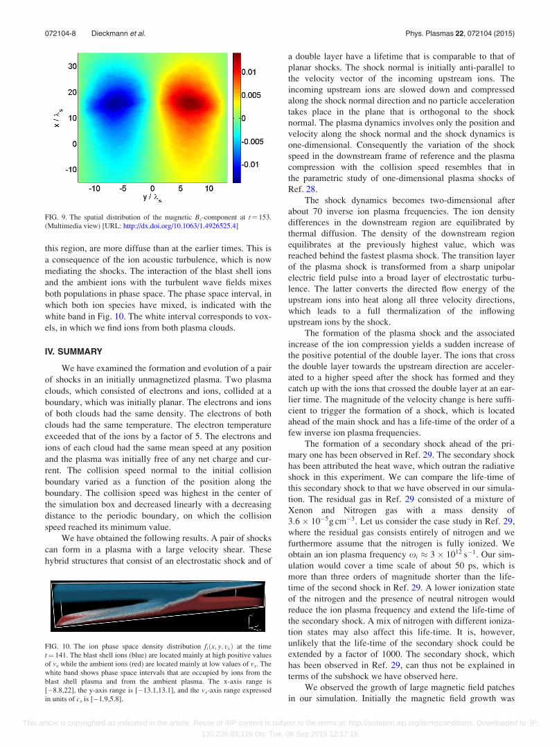
Figure 9 shows the distribution of the magnetic Bz com-

ponent at t¼ 153. The magnetic field patches in Fig. 9 have

expanded along x compared to those at t¼ 70 and their width

along this direction is about 40ks. Their expansion along the

y-direction was already limited by the simulation box size at

t¼ 70 and hence the patches could not expand further along

this direction. The coherence scale of the magnetic field

patches, their expansion far upstream of the shock and their

close correlation with the cusps of the overlap layer exclude

the Weibel instability as the cause. The magnetic fields

driven by the Weibel instability oscillate in space and their

wavelength is comparable to an electron skin depth.

The ion phase space density distribution at t¼ 141 is

shown in Fig. 10. This distribution demonstrates that a

downstream region still exists. The shocks, which enclose

FIG. 6. The ion phase space density distribution fiðx; y; vxÞ at the time

t¼ 70. The blast shell ions (blue) are located mainly at high positive values

of vx while the ambient ions (red) are located mainly at low values of vx. The

x-axis range is [�5.75,12.0], the y-axis range is [�13.1,13.1], and the vx-

axis range expressed in units of cs is [�1.9,5.8]. (Multimedia view) [URL:

http://dx.doi.org/10.1063/1.4926525.1]

FIG. 7. The ion density distribution expressed in units of n0 at the time

t¼ 153. (Multimedia view) [URL: http://dx.doi.org/10.1063/1.4926525.2]

FIG. 8. The spatial distribution of the electric Ex-component at t¼ 153.

(Multimedia view) [URL: http://dx.doi.org/10.1063/1.4926525.3]

072104-7 Dieckmann et al. Phys. Plasmas 22, 072104 (2015)

This article is copyrighted as indicated in the article. Reuse of AIP content is subject to the terms at: http://scitation.aip.org/termsconditions. Downloaded to IP:

130.236.83.116 On: Tue, 08 Sep 2015 12:17:16

this region, are more diffuse than at the earlier times. This is

a consequence of the ion acoustic turbulence, which is now

mediating the shocks. The interaction of the blast shell ions

and the ambient ions with the turbulent wave fields mixes

both populations in phase space. The phase space interval, in

which both ion species have mixed, is indicated with the

white band in Fig. 10. The white interval corresponds to vox-

els, in which we find ions from both plasma clouds.

IV. SUMMARY

We have examined the formation and evolution of a pair

of shocks in an initially unmagnetized plasma. Two plasma

clouds, which consisted of electrons and ions, collided at a

boundary, which was initially planar. The electrons and ions

of both clouds had the same density. The electrons of both

clouds had the same temperature. The electron temperature

exceeded that of the ions by a factor of 5. The electrons and

ions of each cloud had the same mean speed at any position

and the plasma was initially free of any net charge and cur-

rent. The collision speed normal to the initial collision

boundary varied as a function of the position along the

boundary. The collision speed was highest in the center of

the simulation box and decreased linearly with a decreasing

distance to the periodic boundary, on which the collision

speed reached its minimum value.

We have obtained the following results. A pair of shocks

can form in a plasma with a large velocity shear. These

hybrid structures that consist of an electrostatic shock and of

a double layer have a lifetime that is comparable to that of

planar shocks. The shock normal is initially anti-parallel to

the velocity vector of the incoming upstream ions. The

incoming upstream ions are slowed down and compressed

along the shock normal direction and no particle acceleration

takes place in the plane that is orthogonal to the shock

normal. The plasma dynamics involves only the position and

velocity along the shock normal and the shock dynamics is

one-dimensional. Consequently the variation of the shock

speed in the downstream frame of reference and the plasma

compression with the collision speed resembles that in

the parametric study of one-dimensional plasma shocks of

Ref. 28.

The shock dynamics becomes two-dimensional after

about 70 inverse ion plasma frequencies. The ion density

differences in the downstream region are equilibrated by

thermal diffusion. The density of the downstream region

equilibrates at the previously highest value, which was

reached behind the fastest plasma shock. The transition layer

of the plasma shock is transformed from a sharp unipolar

electric field pulse into a broad layer of electrostatic turbu-

lence. The latter converts the directed flow energy of the

upstream ions into heat along all three velocity directions,

which leads to a full thermalization of the inflowing

upstream ions by the shock.

The formation of the plasma shock and the associated

increase of the ion compression yields a sudden increase of

the positive potential of the double layer. The ions that cross

the double layer towards the upstream direction are acceler-

ated to a higher speed after the shock has formed and they

catch up with the ions that crossed the double layer at an ear-

lier time. The magnitude of the velocity change is here suffi-

cient to trigger the formation of a shock, which is located

ahead of the main shock and has a life-time of the order of a

few inverse ion plasma frequencies.

The formation of a secondary shock ahead of the pri-

mary one has been observed in Ref. 29. The secondary shock

has been attributed the heat wave, which outran the radiative

shock in this experiment. We can compare the life-time of

this secondary shock to that we have observed in our simula-

tion. The residual gas in Ref. 29 consisted of a mixture of

Xenon and Nitrogen gas with a mass density of

3:6� 10�5g cm�3. Let us consider the case study in Ref. 29,

where the residual gas consists entirely of nitrogen and we

furthermore assume that the nitrogen is fully ionized. We

obtain an ion plasma frequency xi � 3� 1012 s�1. Our sim-

ulation would cover a time scale of about 50 ps, which is

more than three orders of magnitude shorter than the life-

time of the second shock in Ref. 29. A lower ionization state

of the nitrogen and the presence of neutral nitrogen would

reduce the ion plasma frequency and extend the life-time of

the secondary shock. A mix of nitrogen with different ioniza-

tion states may also affect this life-time. It is, however,

unlikely that the life-time of the secondary shock could be

extended by a factor of 1000. The secondary shock, which

has been observed in Ref. 29, can thus not be explained in

terms of the subshock we have observed here.

We observed the growth of large magnetic field patches

in our simulation. Initially the magnetic field growth was

FIG. 10. The ion phase space density distribution fiðx; y; vxÞ at the time

t¼ 141. The blast shell ions (blue) are located mainly at high positive values

of vx while the ambient ions (red) are located mainly at low values of vx. The

white band shows phase space intervals that are occupied by ions from the

blast shell plasma and from the ambient plasma. The x-axis range is

[�8.8,22], the y-axis range is [�13.1,13.1], and the vx-axis range expressed

in units of cs is [�1.9,5.8].

FIG. 9. The spatial distribution of the magnetic Bz-component at t¼ 153.

(Multimedia view) [URL: http://dx.doi.org/10.1063/1.4926525.4]

072104-8 Dieckmann et al. Phys. Plasmas 22, 072104 (2015)

This article is copyrighted as indicated in the article. Reuse of AIP content is subject to the terms at: http://scitation.aip.org/termsconditions. Downloaded to IP:

130.236.83.116 On: Tue, 08 Sep 2015 12:17:16

limited to the ion cloud overlap layer. Magnetic fields can be

generated via the Weibel instability25 in spatially localized

ion density accumulations such as shocks22 and rarefaction

waves.23,24 The magnetic field structures observed at later

times expanded into the upstream region and they were not

showing spatial oscillations on an electron skin depth-scale,

which are typical for the magnetic fields driven by the

Weibel instability. The magnetic fields were coherent over

tens of electron skin depths and the area they covered was

limited by the dimensions of the simulation box and by the

simulation time. The large-scale magnetic fields started to

grow when the shock normal was no longer aligned with the

plasma flow velocity vector. We have attributed the large

scale magnetic field to currents, which initially develop close

to the cusp in the overlap layer. The simulation shows that

the magnetic field eventually diffuses out of the overlap

layer.

Experimental observations indicate that some SNR

shocks are immersed in magnetic fields with amplitudes that

exceed by far the values one would expect from the shock

compression of the magnetic field of the interstellar me-

dium.30 Cosmic rays can magnetize the interstellar medium

on large spatial scales.31 We scale the growth time of the

magnetic field and the size of the magnetic patches to the

plasma parameters found close to SNR shocks in order to

determine if the corrugation of plasma shocks could be im-

portant for the magnetic field generation at SNR shocks. We

take the reference value 10 cm�3 for the ion number density

close to an SNR shock. Our simulation duration would corre-

spond to �4� 10�2 s. The spatial size �40ks of the mag-

netic field patches would correspond to about 50 km and

their field amplitude would be of the order of 10 nT. The val-

ues for the growth time and the size of the magnetic field

patches are microscopic compared to the size and the evolu-

tion time of an SNR shock. However, the magnetic field am-

plitude generated in our simulation exceeds that of the

interstellar magnetic field by an order of magnitude. A corru-

gated shock front could thus generate magnetic fields ahead

of the shock which are significantly stronger than those of

the interstellar medium and it could compress these as it

propagates across them.

The periodic boundary conditions along the y-direction

have limited the lateral expansion of the magnetic field patch

at late times. An electron, which moves at the thermal speed,

could cross the simulation box several times along the

y-direction during the simulation time. Numerical artifacts,

which are caused by the wrap-around of electrons, can usu-

ally be neglected because the electrons are scattered on the

way by the electrostatic simulation noise.

The key findings of this paper should, however, not be

affected by the periodic boundary conditions. The net current

that drives the magnetic field is generated in a small spatial

interval close to the cusps that is far from the boundaries.

The simulation box geometry will affect the shape of the

generated magnetic field but not its generation mechanism.

The stability of the shocks is also not affected by the bound-

ary conditions because the thermal speed of the ions is not

high enough to let them cross the simulation box during the

simulation time.

ACKNOWLEDGMENTS

The simulations were performed on resources provided

by the Swedish National Infrastructure for Computing

(SNIC) at HPC2N (Umea). GS acknowledges the EPSRC

Grant No. EP/L013975/1. The EPOCH code used in this

research was developed under UK Engineering and Physics

Sciences Research Council Grant Nos. EP/G054940/1, EP/

G055165/1, and EP/G056803/1.

1S. D. Bale, M. A. Balikhin, T. S. Horbury, V. V. Krasnoselskikh, H.

Kucharek, E. M€obius, S. N. Walker, A. Balogh, D. Burgess, B. Lembege,

E. A. Lucek, M. Scholer, S. J. Schwartz, and M. F. Thomsen, Space Sci.

Rev. 118, 161 (2005).2D. Burgess, E. A. Lucek, M. Scholer, S. D. Bale, M. A. Balikhin, A.

Balogh, T. S. Horbury, V. V. Krasnoselskikh, H. Kucharek, B. Lembege,

E. M€obius, S. J. Schwarz, M. F. Thomsen, and S. N. Walker, Space Sci.

Rev. 118, 205 (2005).3M. E. Dieckmann, G. Sarri, D. Doria, H. Ahmed, and M. Borghesi, New J.

Phys. 16, 073001 (2014).4Y. Kazimura, F. Califano, J. I. Sakai, T. Neubert, F. Pegoraro, and S.

Bulanov, J. Phys. Soc. Jpn. 67, 1079 (1998).5J. T. Frederiksen, C. B. Hededal, T. Haugbolle, and A. Nordlund,

Astrophys. J. 608, L13 (2004).6A. Spitkovsky, Astrophys. J. 673, L39 (2008).7A. Stockem, F. Fiuza, A. Bret, R. A. Fonseca, and L. O. Silva, Sci. Rep. 4,

3934 (2014).8D. W. Koopman and D. A. Tidman, Phys. Rev. Lett. 18, 533 (1967).9S. O. Dean, E. A. McLean, J. A. Stamper, and H. R. Griem, Phys. Rev.

Lett. 27, 487 (1971).10A. R. Bell, P. Choi, A. E. Dangor, O. Willi, and D. A. Bassett, Phys. Rev.

A 38, 1363 (1988).11L. Romagnani, S. V. Bulanov, M. Borghesi, P. Audebert, J. C. Gauthier,

K. L€owenbr€uck, A. J. MacKinnon, P. Patel, G. Pretzler, T. Toncian, and

O. Willi, Phys. Rev. Lett. 101, 025004 (2008).12G. Gregori et al., Nature 481, 480 (2012).13H. Ahmed, M. E. Dieckmann, L. Romagnani, D. Doria, G. Sarri, M.

Cerchez, E. Ianni, I. Kourakis, A. L. Giesecke, M. Notley, R. Prasad, K.

Quinn, O. Willi, and M. Borghesi, Phys. Rev. Lett. 110, 205001 (2013).14N. Hershkowitz, J. Geophys. Res. 86, 3307, doi:10.1029/

JA086iA05p03307 (1981).15H. Karimabadi, N. Omidi, and K. B. Quest, Geophys. Res. Lett. 18, 1813,

doi:10.1029/91GL02241 (1991).16T. N. Kato and H. Takabe, Phys. Plasmas 17, 032114 (2010).17D. W. Forslund and C. R. Shonk, Phys. Rev. Lett. 25, 281 (1970).18J. M. Dawson, Rev. Mod. Phys. 55, 403 (1983).19T. H. Dupree, Phys. Fluids 6, 1714 (1963).20G. Sarri, G. C. Murphy, M. E. Dieckmann, A. Bret, K. Quinn, I. Kourakis,

M. Borghesi, L. O. C. Drury, and A. Ynnerman, New J. Phys. 13, 073023

(2011).21K. Eidmann, J. Meyer-ter-Vehn, and T. Schlegel, Phys. Rev. E 62, 1202

(2000).22A. Stockem, T. Grismayer, R. A. Fonseca, and L. O. Silva, Phys. Rev.

Lett. 113, 105002 (2014).23C. Thaury, P. Mora, A. Heron, and J. C. Adam, Phys. Rev. E 82, 016408

(2010).24K. Quinn, L. Romagnani, B. Ramakrishna, G. Sarri, M. E. Dieckmann, P.

A. Wilson, J. Fuchs, L. Lancia, A. Pipahl, T. Toncian, O. Willi, R. J.

Clarke, M. Notley, A. Macchi, and M. Borghesi, Phys. Rev. Lett. 108,

135001 (2012).25E. S. Weibel, Phys. Rev. Lett. 2, 83 (1959).26A. Stockem, M. E. Dieckmann, and R. Schlickeiser, Plasma Phys.

Controlled Fusion 51, 075014 (2009).27D. W. Forslund and J. P. Freidberg, Phys. Rev. Lett. 27, 1189 (1971).28M. E. Dieckmann, H. Ahmed, G. Sarri, D. Doria, I. Kourakis, L.

Romagnani, M. Pohl, and M. Borghesi, Phys. Plasmas 20, 042111 (2013).29J. F. Hansen, M. J. Edwards, D. H. Froula, A. D. Edens, G. Gregori, and T.

Ditmire, Phys. Plasmas 13, 112101 (2006).30E. G. Berezhko, L. T. Ksenofontov, and H. J. Volk, Astron. Astrophys.

412, L11 (2003).31A. R. Bell, Mon. Not. R. Astron. Soc. 353, 550 (2004).

072104-9 Dieckmann et al. Phys. Plasmas 22, 072104 (2015)

This article is copyrighted as indicated in the article. Reuse of AIP content is subject to the terms at: http://scitation.aip.org/termsconditions. Downloaded to IP:

130.236.83.116 On: Tue, 08 Sep 2015 12:17:16