© 2011 ANSYS, Inc. April 27, 2015 1

Shock & Vibration using ANSYS Mechanical

Kelly Morgan ANSYS Inc.

© 2011 ANSYS, Inc. April 27, 2015 2

Outline

1. Introduction to Dynamic Analysis

2. Types of Dynamic Analysis in ANSYS – Modal

– Harmonic

– Transient

– Spectrum

– Random vibrations [PSD]

3. Case Study: Half-Sine Shock on a PCB model

© 2011 ANSYS, Inc. April 27, 2015 3

Definition & Purpose

Determine the dynamic behavior (inertia and possibly damping) of a structure or component.

Why not just Static? It is quick!

What is “Dynamic behavior”?

• Vibration characteristics

– how the structure vibrates and at what frequencies

• Effect of harmonic loads.

• Effect of seismic or shock loads.

• Effect of random loads.

• Effect of time-varying loads.

© 2011 ANSYS, Inc. April 27, 2015 4

Types of Vibrations

Vibrations

Non-deterministic Deterministic

Random Harmonic Transient

Shock

Spectrum

© 2011 ANSYS, Inc. April 27, 2015 5

Types of Dynamic Analysis

Type Input Output

Modal • Prescribed BCs/none • natural frequencies and

corresponding mode shapes

• stress/strain profile

Harmonic • sinusoidally-varying excitations

across a range of frequencies

• sinusoidally-varying response at

each frequency

• min/max response over frequency

range

Spectrum • spectrum representing the

response to a specific time history

• maximum response if the model

were subjected to the time history

Random • spectrum representing probability

distribution of excitation

• response within specified range of

probabilities

Transient • time-varying loads • time-varying response

© 2011 ANSYS, Inc. April 27, 2015 6

Equation of Motion

FuKuCuM

The linear general equation of motion, which will be referred to throughout this course, is as follows (matrix form):

Note that this is simply a force balance:

vectorload applied

nt vectordisplaceme nodalmatrix stiffness structural

vector velocity nodalmatrix damping structural

on vectoraccelerati nodalmatrix mass structural

F

uK

uC

uM

appliedstiffnessdampinginertial FFFF

FuKuCuM

© 2011 ANSYS, Inc. April 27, 2015 7

Modal Analysis

© 2011 ANSYS, Inc. April 27, 2015 8

Description & Purpose

A modal analysis is a technique used to determine the vibration characteristics of structures:

• natural frequencies

– at what frequencies the structure would tend to naturally vibrate

• mode shapes

– in what shape the structure would tend to vibrate at each frequency

• mode participation factors

– the amount of mass that participates in a given direction for each mode

Most fundamental of all the dynamic analysis types.

© 2011 ANSYS, Inc. April 27, 2015 9

Description & Purpose

Benefits of modal analysis

Allows the design to avoid resonant vibrations or to vibrate at a specified frequency (speaker box, for example).

Gives engineers an idea of how the design will respond to different types of dynamic loads.

Helps in calculating solution controls (time steps, etc.) for other dynamic analyses.

Recommendation: Because a structure’s vibration characteristics determine how it responds to any type of dynamic load, it is generally recommended to perform a modal analysis first before trying any other dynamic analysis.

© 2011 ANSYS, Inc. April 27, 2015 10

Eigenvalues & Eigenvectors

• The square roots of the eigenvalues

are wi, the structure’s natural circular

frequencies (rad/s).

• The eigenvectors {f}i represent the

mode shapes, i.e. the shape assumed

by the structure when vibrating at

frequency fi.

mode 1

← {f}1

f1 = 109 Hz

mode 2

← {f}2

f2 = 202 Hz

mode 3

← {f}3

f3 = 249 Hz

© 2011 ANSYS, Inc. April 27, 2015 11

Prestress Effects Tangent Stiffness matrix

Material Stiffness [KiMat]

• For nonlinear materials, only the linear portion is used

• For hyperelastic materials, the tangent material properties at the point of restart are used

Stress Stiffening [KiStressStiffness] / Spin softening [Ki

SpinSoftening]

• Effects included automatically in large deflection analyses

Contact stiffness [KiContact]

• Contact behavior can be changed prior to the modal analysis

fnessStressStif

i

ingSpinSoften

i

essLoadStiffn

i

Contact

i

Mat

i

T

i

KK

KKKK

[KiT]

ti

© 2011 ANSYS, Inc. April 27, 2015 12

Harmonic Analysis

© 2011 ANSYS, Inc. April 27, 2015 13

Definition & Purpose

What is harmonic analysis?

A technique to determine the steady state response of a structure to sinusoidal (harmonic) loads of known frequency.

Input:

• Harmonic loads (forces, pressures, and imposed displacements) of known magnitude and frequency.

• May be multiple loads all at the same frequency. Forces and displacements can be in-phase or out-of phase. Body loads can only be specified with a phase angle of zero.

Output:

• Harmonic displacements at each DOF, usually out of phase with the applied loads.

• Other derived quantities, such as stresses and strains.

© 2011 ANSYS, Inc. April 27, 2015 14

… Definition & Purpose

Harmonic analysis is used in the design of:

Supports, fixtures, and components of rotating equipment such as compressors, engines, pumps, and turbomachinery.

Structures subjected to vortex shedding (swirling motion of fluids) such as turbine blades, airplane wings, bridges, and towers.

Why should you do a harmonic analysis?

To make sure that a given design can withstand sinusoidal loads at different frequencies (e.g, an engine running at different speeds).

To detect resonant response and avoid it if necessary (by using dampers, for example).

© 2011 ANSYS, Inc. April 27, 2015 15

Resonance When the imposed frequency approaches a

natural frequency in the direction of excitation, a phenomenon known as resonance occurs.

• This can be seen in the figures on the right for a 1-DOF system subjected to a harmonic force for various amounts of damping.

The following will be observed:

• an increase in damping decreases the amplitude of the response for all imposed frequencies,

• a small change in damping has a large effect on the response near resonance, and

• the phase angle always passes through ±90° at resonance for any amount of damping.

© 2011 ANSYS, Inc. April 27, 2015 16

Solution Methods

FULL MSUP

• Exact solution. • Approximate solution; accuracy depends in

part on whether an adequate number of

modes have been extracted to represent

the harmonic response.

• Generally slower than MSUP. • Generally faster than FULL.

• Supports all types of loads and boundary

conditions.

• Support nonzero imposed harmonic

displacements through Enforced Motion

• Solution points must be equally distributed

across the frequency domain.

• Solution points may be either equally

distributed across the frequency domain or

clustered about the natural frequencies of

the structure.

• Solves the full system of simultaneous

equations using the Sparse matrix solver for

complex arithmetic.

• Solves an uncoupled system of equations

by performing a linear combination of

orthogonal vectors (mode shapes).

• Prestressing is available for Harmonic Response in Workbench.

© 2011 ANSYS, Inc. April 27, 2015 17

Transient Analysis

© 2011 ANSYS, Inc. April 27, 2015 18

Introduction

Transient structural analyses are needed to evaluate the response of deformable bodies when inertial effects become significant.

• If inertial and damping effects can be ignored, consider performing a linear or nonlinear static analysis instead

• If the loading is purely sinusoidal and the response is linear, a harmonic response analysis is more efficient

• If the bodies can be assumed to be rigid and the kinematics of the system is of interest, rigid dynamic analysis is more cost-effective

• In all other cases, transient structural analyses should be used, as it is the most general type of dynamic analysis

Assembly shown here is from an Autodesk

Inventor sample model

© 2011 ANSYS, Inc. April 27, 2015 19

Implicit vs Explicit Dynamics?

“Implicit” and “Explicit” refer to two types of time integration methods used to perform dynamic simulations

Solution Impact

Velocity (m/s)

Strain Rate

(/s)

Effect

Implicit <10-5 Static / Creep

< 50 10-5 - 10-1 Elastic

50 -1000 10-1 - 101 Elastic-Plastic (material

strength significant)

1000 - 3000 105 - 106

Primarily Plastic

(pressure equals or

exceeds material

strength)

3000 - 12000 106 - 108

Hydrodynamic

(pressure many times

material strength)

Explicit > 12000 > 108 Vaporization of colliding

solids

Transient..

© 2011 ANSYS, Inc. April 27, 2015 20

Implicit vs Explicit Dynamics

Contact

• Implicit dynamics

– All contacts must be defined prior to solve

• Explicit dynamics

– Non-linear contacts do not need to be defined prior to solve

Materials

• Explicit dynamics generally supports more material failure models than implicit dynamics.

Transient..

© 2011 ANSYS, Inc. April 27, 2015 21

Preliminary Modal Analysis

Use automatic time-stepping, proper selection of the initial, minimum, and maximum time steps is important to represent the dynamic response accurately:

• Unlike rigid dynamic analyses which use explicit time integration, transient structural analyses use implicit time integration. Hence, the time steps are usually

larger for transient structural analyses

• The dynamic response can be thought of as various mode shapes of the structure being excited by a loading.

• It is recommended to use automatic time-stepping (default):

– The maximum time step can be chosen based on accuracy concerns. This value can be defined as the same or slightly larger than the initial time step

– The minimum time step can be input to prevent Workbench Mechanical from solving indefinitely (1/100 or 1/1000 of the initial time step)

© 2011 ANSYS, Inc. April 27, 2015 22

… Preliminary Modal Analysis

A general suggestion for selection of the initial time step is to use the following equation:

where fresponse is the frequency of the highest mode of interest

In order to determine the highest mode of interest, a preliminary modal analysis should be performed prior to the transient structural analysis

• mode shapes of the structure are known

• value of fresponse value determine

• It is a good idea to examine the various mode shapes to determine which frequency may be the highest mode of interest contributing to the response of the structure.

response

initialf

t20

1

© 2011 ANSYS, Inc. April 27, 2015 23

Initial Conditions

For a transient structural analysis, initial displacement and initial velocity is required:

• User can define initial conditions via “Initial Condition” branch or by using multiple Steps

Defining initial displacement & velocity with the “Initial Condition” object:

• Default condition is that all bodies are at rest

• If some bodies have zero initial displacement but non-zero constant initial velocity, this can be input

– Only bodies can be specified

– Enter constant initial velocity (Cannot specify more than one constant velocity value with this method)

© 2011 ANSYS, Inc. April 27, 2015 24

Time-Varying Loads

Structural loads and joint conditions can be input as time-dependent load histories

• When adding a Load or Joint Condition, the magnitude can be defined as a constant, tabular value, or function.

• The values can be entered directly in the Workbench Mechanical GUI

Transient..

© 2011 ANSYS, Inc. April 27, 2015 25

Response Spectrum Analysis

© 2011 ANSYS, Inc. April 27, 2015 26

Description & Purpose

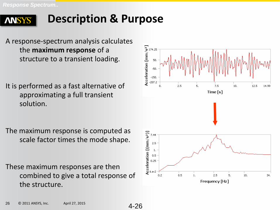
A response-spectrum analysis calculates the maximum response of a structure to a transient loading.

It is performed as a fast alternative of approximating a full transient solution.

The maximum response is computed as scale factor times the mode shape.

These maximum responses are then combined to give a total response of the structure.

4-26

Response Spectrum..

© 2011 ANSYS, Inc. April 27, 2015 27

Description & Purpose

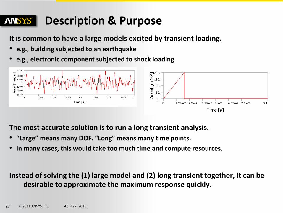
It is common to have a large models excited by transient loading.

• e.g., building subjected to an earthquake

• e.g., electronic component subjected to shock loading

The most accurate solution is to run a long transient analysis.

• “Large” means many DOF. “Long” means many time points.

• In many cases, this would take too much time and compute resources.

Instead of solving the (1) large model and (2) long transient together, it can be desirable to approximate the maximum response quickly.

© 2011 ANSYS, Inc. April 27, 2015 28

Common Uses

Commonly used in the analysis of:

• Electronic equipment for shock loading

• Nuclear power plant buildings and components, for seismic loading

• Commercial buildings in earthquake zones

Types of Response Spectrum analysis:

Single-point response spectrum

• A single response spectrum excites all specified points in the model.

Multi-point response spectrum

• Different response spectra excite different points in the model.

Response Spectrum..

© 2011 ANSYS, Inc. April 27, 2015 29

Spectral Regions

These two frequencies can often be identified on a response spectrum

• This divides the spectrum into three regions mid

frequency

high

frequency

low

frequency

fSP

frequency at peak response

(spectral peak)

fZPA

frequency at rigid response

(zero period acceleration)

1. Low frequency (below fSP)

• periodic region

• modes are periodic & generally uncorrelated unless closely spaced

2. Mid frequency (between fSP and fZPA)

• transition from periodic to rigid

• modes have periodic component and rigid component

3. High Frequency (above fZPA)

• rigid region

• modes correlated with input frequency and, therefore, also with themselves

ZPA

© 2011 ANSYS, Inc. April 27, 2015 30

Recommended Solution Procedure

The recommended solution method is generally specified by your design code.

• combination method

• rigid response method

• missing mass effects

Alternatively, the best solution method can be determined by

• extracting the modes to be used for combination and

• comparing them to the response spectrum

ω1 ω2 ω3 ω4 ω5 ω6 ω7 ω8

© 2011 ANSYS, Inc. April 27, 2015 31

Recommended Solution Procedure

Modes only in low-frequency region

• SRSS (or CQC/ROSE for closely spaced modes).

• No rigid response effects. No missing mass effects.

Modes only in mid- to high-frequency region

• SRSS (or CQC/ROSE for closely spaced modes).

• Rigid response by Lindley or Gupta method. Missing mass on.

Modes in all frequency regions

• SRSS (or CQC/ROSE for closely spaced modes).

• Rigid response by Gupta method. Missing mass on.

ω1 ω2 ω3 ω4 ω5 ω6 ω7 ω8

© 2011 ANSYS, Inc. April 27, 2015 32

Multi-Point Response Spectrum

In multi-point response spectrum (MPRS), different constrained points can be being subjected to different spectra (up to 100 different excitations).

© 2011 ANSYS, Inc. April 27, 2015 33

Random Vibration

© 2011 ANSYS, Inc. April 27, 2015 34

Definition and Purpose

Many common processes result in random vibration

• Parts on a manufacturing line

• Vehicles travelling on a roadway

• Airplanes flying or taxiing

• Spacecraft during launch

The amplitudes at these frequencies vary randomly with time.

• We need some way of describing and quantifying this excitation.

Courtesy: NASA

© 2011 ANSYS, Inc. April 27, 2015 35

Assumptions & Restrictions

The structure has

• no random properties

• no time varying stiffness, damping, or mass

• no time varying forces, displacement, pressures, temperatures, etc applied

• light damping

– damping forces are much smaller than inertial and elastic forces

The random process is

• stationary (does not change with time)

– the response will also be a stationary random process

• ergodic (one sample tells us everything about the random process)

© 2011 ANSYS, Inc. April 27, 2015 36

Random Vibration

To calculate the response PSD (RPSD), multiply the input PSD by the response function

ww in

in

outout S

a

aS

2

or PSDinput RPSD

2

in

out

a

a

© 2011 ANSYS, Inc. April 27, 2015 37

Random Vibration

For real models with multiple DOFs

• RPSDs are calculated for every node in every free direction at each frequency

– RPSDs can be plotted for each node in a specific direction versus frequency

• a RMS value (sigma value) for the entire frequency range is calculated for every node in every free direction

– sigma values can be plotted as a contour for the entire model for a specific direction.

Z direction

© 2011 ANSYS, Inc. April 27, 2015 38

Shock Analysis using Transient & Response Spectrum

Kelly Morgan

ANSYS Inc.

© 2011 ANSYS, Inc. April 27, 2015 39

Methods for Shock Analysis

Response Spectrum Method

• Commonly used for large models

• Solve much faster than a full transient analysis

• Includes non-stationary excitations

• Linear analysis only

Transient (Time History Analysis)

• Include non-stationary and non-linear analysis

• Computationally quite expensive

© 2011 ANSYS, Inc. April 27, 2015 40

PCB model details

Basic guidelines for performing shock analysis based on Implicit Transient as well as Response spectrum in ANSYS WB is used

A real life example of a PCB subjected to standard 30g-11ms-half sine shock is considered as the basis of the study.

Different parameters like results, memory requirements, solution time required for both the Transient & RS are compared.

Quarter symmetry model is taken

Quarter symmetric PCB Shock load

Transient..

© 2011 ANSYS, Inc. April 27, 2015 41

Define Materials, BCs, Loads:

Material properties of different components are defined in ‘Engineering data’.

Transient analysis is done for a total time of 2.5e-2sec.

Initial conditions: Zero displacement and zero initial velocity.

• Fixed BC: The cantilever is fixed at one end.

• Acceleration Shock load: 30g-11ms, Half-sine shock pulse in transverse, z-dirn.

Transient..

Transient shock-load input data

© 2011 ANSYS, Inc. April 27, 2015 42

Analysis settings and time step definitions

Load steps, end time, time step size, damping, etc. are defined in the Analysis settings.

Including non-linear effects or not can also be defined.

Time step size is very crucial in Transient analysis as it determines the no. of dynamic modes one can capture.

• 1st, 4th,5th mode freqs.=311, 3161, 4371 Hz, respectively.

• To capture 4th mode time step should be around (1/20*3161)=1.58e-5s. 1e-4 is taken as the time step for solution.

Transient..

© 2011 ANSYS, Inc. April 27, 2015 43

Spectrum analysis for Half-sine shock Response Spectrum..

Project Schematic Mechanical outline of Spectrum analysis

© 2011 ANSYS, Inc. April 27, 2015 44

Converting Time domain load into Spectrum input

Time domain data can be converted into Spectrum data (Freq domain) through RESP command in ANSYS:

0

100

200

300

400

500

600

0 500 1000 1500 2000 2500

Series1

RESP

command

Response Spectrum..

Time domain data

(Transient analysis) Frequency domain data

(Response Spectrum)

© 2011 ANSYS, Inc. April 27, 2015 45

Applying acceleration Spectrum input in Spectrum analysis

Response Spectrum..

RS acceleration input data Settings of RS analysis

© 2011 ANSYS, Inc. April 27, 2015 46

Transient versus RS

Maximum deformation, Normal & Shear stress are compared from the Transient & the RS analysis.

Transient results are assumed to be accurate and benchmark for accessing RS results.

Time taken for both the analysis are compared

© 2011 ANSYS, Inc. April 27, 2015 47

Results comparison- Maximum

Transient Normal stress_x-dirn (Max=-3663.7 psi) RS Normal stress_x-dirn (Max= 3630.1 psi)

Transient directional deformation in z-dirn (Max= -4.2093 in) RS directional deformation in z-dirn (Max= 4.5962e-3 in)

© 2011 ANSYS, Inc. April 27, 2015 48

Results comparison- Maximum Normal Stress

Transient Normal stress_y-dirn (Max= -1350.3 psi)

Transient Normal stress_z-dirn (Max= -1991.9 psi)

RS Normal stress_y-dirn (Max=1509.1 psi)

RS Normal stress_z-dirn (Max=2261.5 psi)

© 2011 ANSYS, Inc. April 27, 2015 49

Results comparison- Shear stresses

Transient Shear stress_xy-dirn (Max= -568.68 psi) RS Shear stress_xy-dirn (Max= 611.3 psi)

Transient Shear stress_xz-dirn (Max= 1742.4 psi) RS shear stress_xz-dirn (Max= 1993.1 psi)

© 2011 ANSYS, Inc. April 27, 2015 50

Results comparison- Shear stresses

Transient Shear stress_yz-dirn (Max= -529.83 psi) RS Shear stress_yz-dirn (Max= 589.16 psi)

Results summary:

•Results from RS are within 14% of the Transient results.

•As in RS, only absolute values of result quantities are taken, the plot colors

look different. But considering only absolute values in Transient, the plots in

RS & transient are comparable.

•Critical locations (high stress regions) are correctly predicted by RS.

© 2011 ANSYS, Inc. April 27, 2015 51

Final observations & comments

The RS results are in reasonable limits of the Transient results.

The elapsed time in RS is quite less (125 times less in PCB model) than in the Transient run.

The time advantage is even more for big models, with contacts & complicated load histories typical in earthquakes, which justifies RS use in Shock and Earthquake analysis even at cost of some accuracy.

Comparison of different results in Transient vs RS

Result (Max)

Z-dirn deformation-(inch)

X-Normal Stress –(psi)

Y-Normal Stress –(psi)

Z-Normal Stress –(psi)

XY-Shear Stress –(psi)

YZ-Shear Stress –(psi)

ZX-Shear Stress –(psi)

CP Time –(sec)

Full Transient

-4.2093 e-3

- 3663.7 -1350.3 1991.9 - 568.68 1742.4 - 529.83 7192

MSUP Transient

-4.1766e-003

-3485.3 psi 49+136= 185

Spectrum (CQC)

4.5962e-3 3630.1 1509.1 2261.5 611.3 1993.1 589.16 49+8.375= 57.375

Percentage difference

9 0.09 11.3 13.5 7.4 14 11.1 7192/57.375= 125 times

© 2011 ANSYS, Inc. April 27, 2015 52

Comments for usage in industry

When to go for Shock analysis using Response Spectrum?

• In industry, detailed, expensive analysis like Transient are not always necessary.

• For example, many times quick analysis of the systems is more important, even though if it comes with some compromise on accuracy.

• Also such quick analysis can be a basis for selection from a number of designs, and then carrying out detailed analysis of selected few.

• Detailed Transient analysis is nearly impossible, For example Seismic analysis of a complex component.

When to go for Shock analysis using implicit Transient ?

• When non-linearities play such an important role that they cannot be ignored for correct behavior of the model.

• Carrying out detailed analysis on selected specimens (based on prior analysis like RS) to finalize the design.

• When reliability of a particular design is very critical and accuracy is indispensible.

© 2011 ANSYS, Inc. April 27, 2015 53

Thank You

© 2011 ANSYS, Inc. April 27, 2015 54

Q/A