An Introduction to Reinforcement Learning

Shivaram Kalyanakrishnan

shivaram@csa.iisc.ernet.in

Department of Computer Science and Automation

Indian Institute of Science

August 2014

What is Reinforcement Learning?

Shivaram Kalyanakrishnan 1/19

What is Reinforcement Learning?

[Video1 of little girl learning to ride bicycle]

1. https://www.youtube.com/watch?v=Qv43pKlVZXk

Shivaram Kalyanakrishnan 1/19

What is Reinforcement Learning?

[Video1 of little girl learning to ride bicycle]

1. https://www.youtube.com/watch?v=Qv43pKlVZXk

Shivaram Kalyanakrishnan 1/19

What is Reinforcement Learning?

[Video1 of little girl learning to ride bicycle]

Learning to Drive a Bicycle using Reinforcement Learning and Shaping

Jette Randløv and Preben Alstrøm. ICML 1998.

1. https://www.youtube.com/watch?v=Qv43pKlVZXk

Shivaram Kalyanakrishnan 1/19

What is Reinforcement Learning?

[Video1 of little girl learning to ride bicycle]

Learning to Drive a Bicycle using Reinforcement Learning and Shaping

Jette Randløv and Preben Alstrøm. ICML 1998.

Learning by trial and error to perform sequential decision making.

1. https://www.youtube.com/watch?v=Qv43pKlVZXk

Shivaram Kalyanakrishnan 1/19

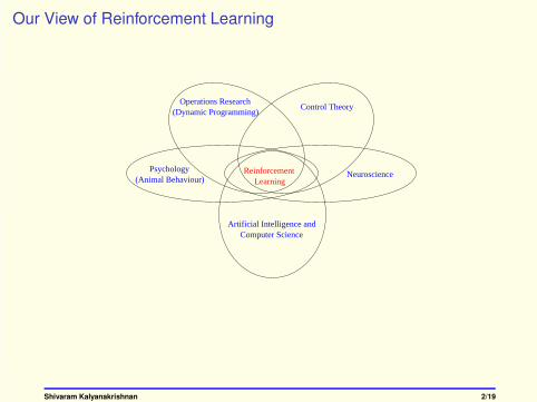
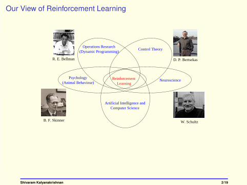
Our View of Reinforcement Learning

NeuroscienceReinforcementLearning

Psychology

Artificial Intelligence andComputer Science

(Animal Behaviour)

Operations Research (Dynamic Programming)

Control Theory

Shivaram Kalyanakrishnan 2/19

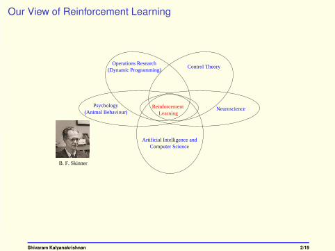
Our View of Reinforcement Learning

NeuroscienceReinforcementLearning

Psychology

Artificial Intelligence andComputer Science

(Animal Behaviour)

Operations Research (Dynamic Programming)

Control Theory

B. F. Skinner

Shivaram Kalyanakrishnan 2/19

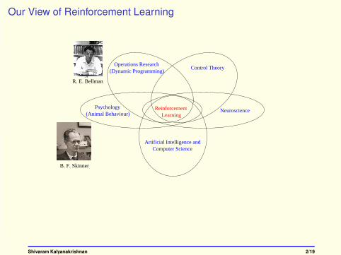
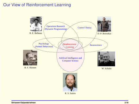
Our View of Reinforcement Learning

NeuroscienceReinforcementLearning

Psychology

Artificial Intelligence andComputer Science

(Animal Behaviour)

Operations Research (Dynamic Programming)

Control Theory

B. F. Skinner

R. E. Bellman

Shivaram Kalyanakrishnan 2/19

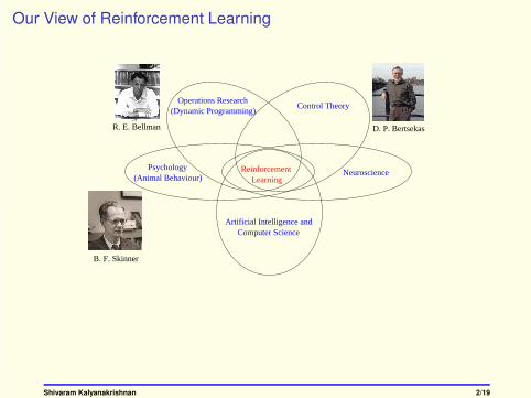
Our View of Reinforcement Learning

NeuroscienceReinforcementLearning

Psychology

Artificial Intelligence andComputer Science

(Animal Behaviour)

Operations Research (Dynamic Programming)

Control Theory

B. F. Skinner

D. P. BertsekasR. E. Bellman

Shivaram Kalyanakrishnan 2/19

Our View of Reinforcement Learning

NeuroscienceReinforcementLearning

Psychology

Artificial Intelligence andComputer Science

(Animal Behaviour)

Operations Research (Dynamic Programming)

Control Theory

B. F. Skinner

D. P. Bertsekas

W. Schultz

R. E. Bellman

Shivaram Kalyanakrishnan 2/19

Our View of Reinforcement Learning

NeuroscienceReinforcementLearning

Psychology

Artificial Intelligence andComputer Science

(Animal Behaviour)

Operations Research (Dynamic Programming)

Control Theory

R. S. Sutton

B. F. Skinner

D. P. Bertsekas

W. Schultz

R. E. Bellman

Shivaram Kalyanakrishnan 2/19

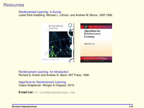
Resources

Reinforcement Learning: A Survey.Leslie Pack Kaelbling, Michael L. Littman, and Andrew W. Moore. JAIR 1996.

Shivaram Kalyanakrishnan 3/19

Resources

Reinforcement Learning: A Survey.Leslie Pack Kaelbling, Michael L. Littman, and Andrew W. Moore. JAIR 1996.

Reinforcement Learning: An IntroductionRichard S. Sutton and Andrew G. Barto. MIT Press, 1998.

Algorithms for Reinforcement LearningCsaba Szepesvári. Morgan & Claypool, 2010.

Shivaram Kalyanakrishnan 3/19

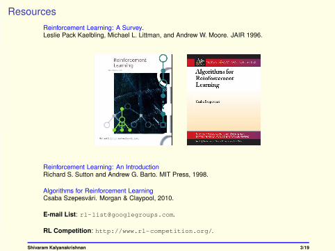
Resources

Reinforcement Learning: A Survey.Leslie Pack Kaelbling, Michael L. Littman, and Andrew W. Moore. JAIR 1996.

Reinforcement Learning: An IntroductionRichard S. Sutton and Andrew G. Barto. MIT Press, 1998.

Algorithms for Reinforcement LearningCsaba Szepesvári. Morgan & Claypool, 2010.

E-mail List: rl-list@googlegroups.com.

Shivaram Kalyanakrishnan 3/19

Resources

Reinforcement Learning: A Survey.Leslie Pack Kaelbling, Michael L. Littman, and Andrew W. Moore. JAIR 1996.

Reinforcement Learning: An IntroductionRichard S. Sutton and Andrew G. Barto. MIT Press, 1998.

Algorithms for Reinforcement LearningCsaba Szepesvári. Morgan & Claypool, 2010.

E-mail List: rl-list@googlegroups.com.

RL Competition: http://www.rl-competition.org/.

Shivaram Kalyanakrishnan 3/19

Today’s Class

1. Markov decision problems

2. Bellman’s (Optimality) Equations, planning and learning

3. Challenges

4. Summary

Shivaram Kalyanakrishnan 4/19

Today’s Class

1. Markov decision problems

2. Bellman’s (Optimality) Equations, planning and learning

3. Challenges

4. Summary

Shivaram Kalyanakrishnan 4/19

Markov Decision Problem

at

st+1

rt+1

st rt

S A

ENVIRONMENT

π :

action

LEARNING AGENT

T

R

state reward

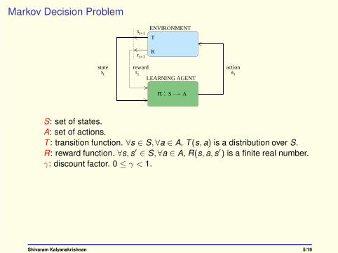
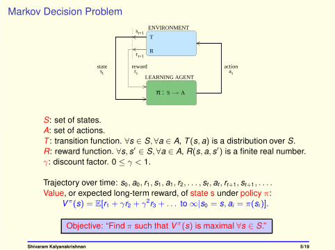
S: set of states.

A: set of actions.

T : transition function. ∀s ∈ S,∀a ∈ A, T (s, a) is a distribution over S.

R: reward function. ∀s, s′ ∈ S,∀a ∈ A, R(s, a, s′) is a finite real number.

γ: discount factor. 0 ≤ γ < 1.

Shivaram Kalyanakrishnan 5/19

Markov Decision Problem

at

st+1

rt+1

st rt

S A

ENVIRONMENT

π :

action

LEARNING AGENT

T

R

state reward

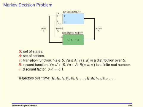
S: set of states.

A: set of actions.

T : transition function. ∀s ∈ S,∀a ∈ A, T (s, a) is a distribution over S.

R: reward function. ∀s, s′ ∈ S,∀a ∈ A, R(s, a, s′) is a finite real number.

γ: discount factor. 0 ≤ γ < 1.

Trajectory over time: s0, a0, r1, s1, a1, r2, . . . , st , at , rt+1, st+1, . . . .

Shivaram Kalyanakrishnan 5/19

Markov Decision Problem

at

st+1

rt+1

st rt

S A

ENVIRONMENT

π :

action

LEARNING AGENT

T

R

state reward

S: set of states.

A: set of actions.

T : transition function. ∀s ∈ S,∀a ∈ A, T (s, a) is a distribution over S.

R: reward function. ∀s, s′ ∈ S,∀a ∈ A, R(s, a, s′) is a finite real number.

γ: discount factor. 0 ≤ γ < 1.

Trajectory over time: s0, a0, r1, s1, a1, r2, . . . , st , at , rt+1, st+1, . . . .

Value, or expected long-term reward, of state s under policy π:

Vπ(s) = E[r1 + γr2 + γ2r3 + . . . to∞|s0 = s, ai = π(si)].

Shivaram Kalyanakrishnan 5/19

Markov Decision Problem

at

st+1

rt+1

st rt

S A

ENVIRONMENT

π :

action

LEARNING AGENT

T

R

state reward

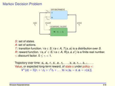
S: set of states.

A: set of actions.

T : transition function. ∀s ∈ S,∀a ∈ A, T (s, a) is a distribution over S.

R: reward function. ∀s, s′ ∈ S,∀a ∈ A, R(s, a, s′) is a finite real number.

γ: discount factor. 0 ≤ γ < 1.

Trajectory over time: s0, a0, r1, s1, a1, r2, . . . , st , at , rt+1, st+1, . . . .

Value, or expected long-term reward, of state s under policy π:

Vπ(s) = E[r1 + γr2 + γ2r3 + . . . to∞|s0 = s, ai = π(si)].

Objective: “Find π such that Vπ(s) is maximal ∀s ∈ S.”

Shivaram Kalyanakrishnan 5/19

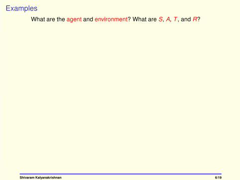
Examples

What are the agent and environment? What are S, A, T , and R?

Shivaram Kalyanakrishnan 6/19

Examples

What are the agent and environment? What are S, A, T , and R?

1. http://www.chess-game-strategies.com/images/kqa_chessboard_large-picture_2d.gif

Shivaram Kalyanakrishnan 6/19

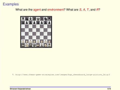
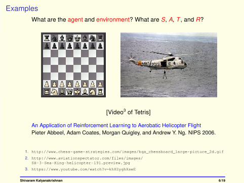
Examples

What are the agent and environment? What are S, A, T , and R?

An Application of Reinforcement Learning to Aerobatic Helicopter Flight

Pieter Abbeel, Adam Coates, Morgan Quigley, and Andrew Y. Ng. NIPS 2006.

1. http://www.chess-game-strategies.com/images/kqa_chessboard_large-picture_2d.gif

2. http://www.aviationspectator.com/files/images/

SH-3-Sea-King-helicopter-191.preview.jpg

Shivaram Kalyanakrishnan 6/19

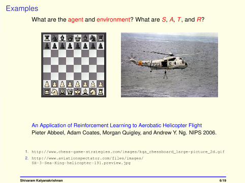
Examples

What are the agent and environment? What are S, A, T , and R?

[Video3 of Tetris]

An Application of Reinforcement Learning to Aerobatic Helicopter Flight

Pieter Abbeel, Adam Coates, Morgan Quigley, and Andrew Y. Ng. NIPS 2006.

1. http://www.chess-game-strategies.com/images/kqa_chessboard_large-picture_2d.gif

2. http://www.aviationspectator.com/files/images/

SH-3-Sea-King-helicopter-191.preview.jpg

3. https://www.youtube.com/watch?v=khHZyghXseE

Shivaram Kalyanakrishnan 6/19

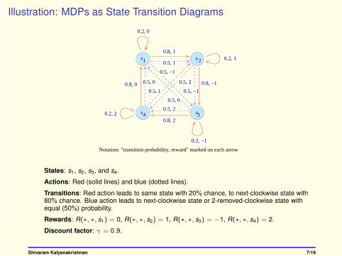
Illustration: MDPs as State Transition Diagrams

s s

s s

1 2

34

Notation: "transition probability, reward" marked on each arrow

0.2, 0

0.8, 10.2, 1

0.8, −1

0.2, −1

0.8, 20.2, 2

0.8, 0

0.5, 1

0.5, −1

0.5, −1

0.5, 2

0.5, 2

0.5, 0

0.5, 0

0.5, 1

States: s1 , s2, s3, and s4 .

Actions: Red (solid lines) and blue (dotted lines).

Transitions: Red action leads to same state with 20% chance, to next-clockwise state with80% chance. Blue action leads to next-clockwise state or 2-removed-clockwise state withequal (50%) probability.

Rewards: R(∗, ∗, s1) = 0, R(∗, ∗, s2) = 1, R(∗, ∗, s3) = −1, R(∗, ∗, s4) = 2.

Discount factor: γ = 0.9.

Shivaram Kalyanakrishnan 7/19

Today’s Class

1. Markov decision problems

2. Bellman’s (Optimality) Equations, planning and learning

3. Challenges

4. Summary

Shivaram Kalyanakrishnan 8/19

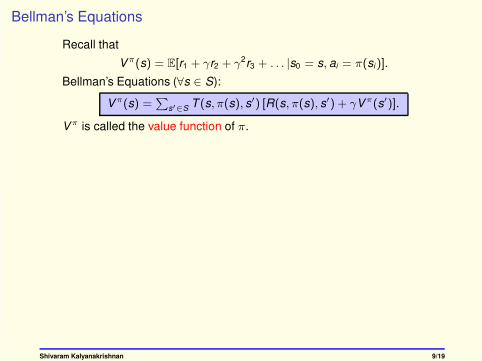
Bellman’s Equations

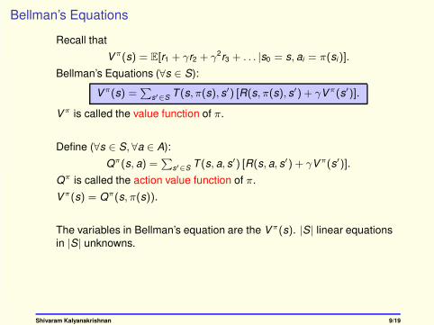
Recall that

Vπ(s) = E[r1 + γr2 + γ2r3 + . . . |s0 = s, ai = π(si)].

Bellman’s Equations (∀s ∈ S):

Vπ(s) =∑

s′∈S T (s, π(s), s′) [R(s, π(s), s′) + γVπ(s′)].

Vπ is called the value function of π.

Shivaram Kalyanakrishnan 9/19

Bellman’s Equations

Recall that

Vπ(s) = E[r1 + γr2 + γ2r3 + . . . |s0 = s, ai = π(si)].

Bellman’s Equations (∀s ∈ S):

Vπ(s) =∑

s′∈S T (s, π(s), s′) [R(s, π(s), s′) + γVπ(s′)].

Vπ is called the value function of π.

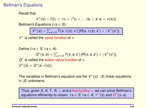
Define (∀s ∈ S, ∀a ∈ A):

Qπ(s, a) =∑

s′∈S T (s, a, s′) [R(s, a, s′) + γVπ(s′)].

Qπ is called the action value function of π.

Vπ(s) = Qπ(s, π(s)).

Shivaram Kalyanakrishnan 9/19

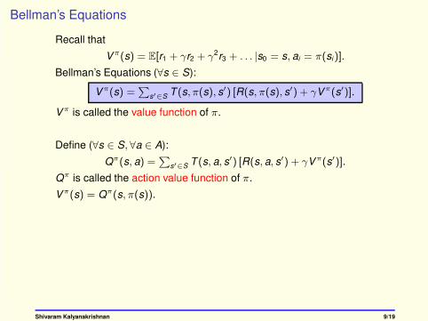
Bellman’s Equations

Recall that

Vπ(s) = E[r1 + γr2 + γ2r3 + . . . |s0 = s, ai = π(si)].

Bellman’s Equations (∀s ∈ S):

Vπ(s) =∑

s′∈S T (s, π(s), s′) [R(s, π(s), s′) + γVπ(s′)].

Vπ is called the value function of π.

Define (∀s ∈ S, ∀a ∈ A):

Qπ(s, a) =∑

s′∈S T (s, a, s′) [R(s, a, s′) + γVπ(s′)].

Qπ is called the action value function of π.

Vπ(s) = Qπ(s, π(s)).

The variables in Bellman’s equation are the Vπ(s). |S| linear equations

in |S| unknowns.

Shivaram Kalyanakrishnan 9/19

Bellman’s Equations

Recall that

Vπ(s) = E[r1 + γr2 + γ2r3 + . . . |s0 = s, ai = π(si)].

Bellman’s Equations (∀s ∈ S):

Vπ(s) =∑

s′∈S T (s, π(s), s′) [R(s, π(s), s′) + γVπ(s′)].

Vπ is called the value function of π.

Define (∀s ∈ S, ∀a ∈ A):

Qπ(s, a) =∑

s′∈S T (s, a, s′) [R(s, a, s′) + γVπ(s′)].

Qπ is called the action value function of π.

Vπ(s) = Qπ(s, π(s)).

The variables in Bellman’s equation are the Vπ(s). |S| linear equations

in |S| unknowns.

Thus, given S, A, T , R, γ, and a fixed policy π, we can solve Bellman’s

equations efficiently to obtain, ∀s ∈ S,∀a ∈ A, Vπ(s) and Qπ(s, a).

Shivaram Kalyanakrishnan 9/19

Bellman’s Optimality Equations

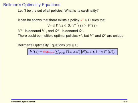
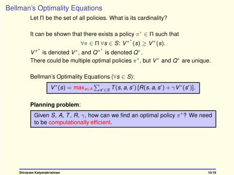
Let Π be the set of all policies. What is its cardinality?

Shivaram Kalyanakrishnan 10/19

Bellman’s Optimality Equations

Let Π be the set of all policies. What is its cardinality?

It can be shown that there exists a policy π∗ ∈ Π such that

∀π ∈ Π ∀s ∈ S: Vπ∗

(s) ≥ Vπ(s).

Vπ∗

is denoted V ∗, and Qπ∗

is denoted Q∗.

There could be multiple optimal policies π∗, but V ∗ and Q∗ are unique.

Shivaram Kalyanakrishnan 10/19

Bellman’s Optimality Equations

Let Π be the set of all policies. What is its cardinality?

It can be shown that there exists a policy π∗ ∈ Π such that

∀π ∈ Π ∀s ∈ S: Vπ∗

(s) ≥ Vπ(s).

Vπ∗

is denoted V ∗, and Qπ∗

is denoted Q∗.

There could be multiple optimal policies π∗, but V ∗ and Q∗ are unique.

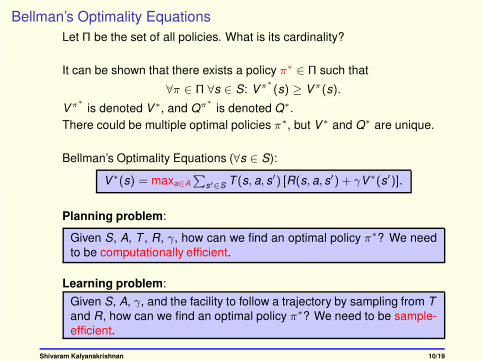
Bellman’s Optimality Equations (∀s ∈ S):

V ∗(s) = maxa∈A

∑s′∈S T (s, a, s′) [R(s, a, s′) + γV ∗(s′)].

Shivaram Kalyanakrishnan 10/19

Bellman’s Optimality Equations

Let Π be the set of all policies. What is its cardinality?

It can be shown that there exists a policy π∗ ∈ Π such that

∀π ∈ Π ∀s ∈ S: Vπ∗

(s) ≥ Vπ(s).

Vπ∗

is denoted V ∗, and Qπ∗

is denoted Q∗.

There could be multiple optimal policies π∗, but V ∗ and Q∗ are unique.

Bellman’s Optimality Equations (∀s ∈ S):

V ∗(s) = maxa∈A

∑s′∈S T (s, a, s′) [R(s, a, s′) + γV ∗(s′)].

Planning problem:

Given S, A, T , R, γ, how can we find an optimal policy π∗? We need

to be computationally efficient.

Shivaram Kalyanakrishnan 10/19

Bellman’s Optimality Equations

Let Π be the set of all policies. What is its cardinality?

It can be shown that there exists a policy π∗ ∈ Π such that

∀π ∈ Π ∀s ∈ S: Vπ∗

(s) ≥ Vπ(s).

Vπ∗

is denoted V ∗, and Qπ∗

is denoted Q∗.

There could be multiple optimal policies π∗, but V ∗ and Q∗ are unique.

Bellman’s Optimality Equations (∀s ∈ S):

V ∗(s) = maxa∈A

∑s′∈S T (s, a, s′) [R(s, a, s′) + γV ∗(s′)].

Planning problem:

Given S, A, T , R, γ, how can we find an optimal policy π∗? We need

to be computationally efficient.

Learning problem:

Given S, A, γ, and the facility to follow a trajectory by sampling from T

and R, how can we find an optimal policy π∗? We need to be sample-

efficient.

Shivaram Kalyanakrishnan 10/19

Planning

Given S, A, T , R, γ, how can we find an optimal policy π∗?

Shivaram Kalyanakrishnan 11/19

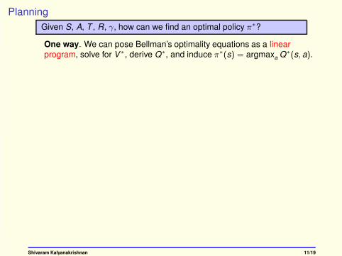
Planning

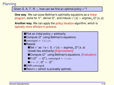
Given S, A, T , R, γ, how can we find an optimal policy π∗?

One way. We can pose Bellman’s optimality equations as a linear

program, solve for V ∗, derive Q∗, and induce π∗(s) = argmaxa Q∗(s, a).

Shivaram Kalyanakrishnan 11/19

Planning

Given S, A, T , R, γ, how can we find an optimal policy π∗?

One way. We can pose Bellman’s optimality equations as a linear

program, solve for V ∗, derive Q∗, and induce π∗(s) = argmaxa Q∗(s, a).

Another way. We can apply the policy iteration algorithm, which is

typically more efficient in practice.

�Pick an initial policy π arbitrarily.

�Compute Qπ using Bellman’s equations.

�converged← false.

�Repeat

�Set π′ as: ∀s ∈ S, π′(s) = argmaxa Qπ(s, a)(break ties arbitrarily).[Improvement]

�Compute Qπ′

using Bellman’s equations. [Evaluation]

�If (Qπ′

= Qπ), converged← true.

�π ← π′, Qπ ← Qπ

′

.

�Until converged.

�Return π (which is provably optimal).

Shivaram Kalyanakrishnan 11/19

Planning

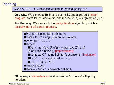
Given S, A, T , R, γ, how can we find an optimal policy π∗?

One way. We can pose Bellman’s optimality equations as a linear

program, solve for V ∗, derive Q∗, and induce π∗(s) = argmaxa Q∗(s, a).

Another way. We can apply the policy iteration algorithm, which is

typically more efficient in practice.

�Pick an initial policy π arbitrarily.

�Compute Qπ using Bellman’s equations.

�converged← false.

�Repeat

�Set π′ as: ∀s ∈ S, π′(s) = argmaxa Qπ(s, a)(break ties arbitrarily).[Improvement]

�Compute Qπ′

using Bellman’s equations. [Evaluation]

�If (Qπ′

= Qπ), converged← true.

�π ← π′, Qπ ← Qπ

′

.

�Until converged.

�Return π (which is provably optimal).

Other ways. Value iteration and its various “mixtures” with policy

iteration.

Shivaram Kalyanakrishnan 11/19

Learning

Given S, A, γ, and the facility to follow a trajectory by sampling from T

and R, how can we find an optimal policy π∗?

Shivaram Kalyanakrishnan 12/19

Learning

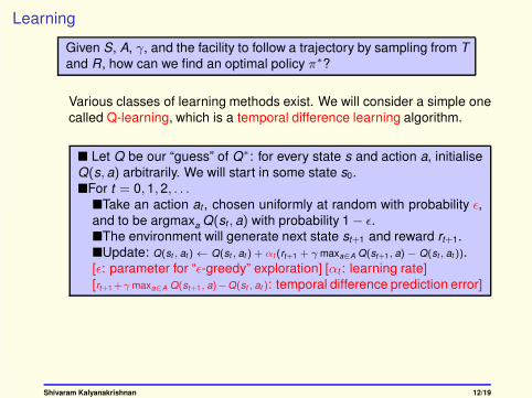
Given S, A, γ, and the facility to follow a trajectory by sampling from T

and R, how can we find an optimal policy π∗?

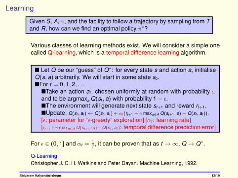
Various classes of learning methods exist. We will consider a simple one

called Q-learning, which is a temporal difference learning algorithm.

� Let Q be our “guess” of Q∗: for every state s and action a, initialise

Q(s, a) arbitrarily. We will start in some state s0.

�For t = 0, 1, 2, . . .

�Take an action at , chosen uniformly at random with probability ǫ,

and to be argmaxa Q(st , a) with probability 1− ǫ.

�The environment will generate next state st+1 and reward rt+1.

�Update: Q(st , at )← Q(st , at ) + αt (rt+1 + γ maxa∈A Q(st+1, a) − Q(st , at )).

[ǫ: parameter for “ǫ-greedy” exploration] [αt : learning rate]

[rt+1+γ maxa∈A Q(st+1, a)−Q(st , at ): temporal difference prediction error]

Shivaram Kalyanakrishnan 12/19

Learning

Given S, A, γ, and the facility to follow a trajectory by sampling from T

and R, how can we find an optimal policy π∗?

Various classes of learning methods exist. We will consider a simple one

called Q-learning, which is a temporal difference learning algorithm.

� Let Q be our “guess” of Q∗: for every state s and action a, initialise

Q(s, a) arbitrarily. We will start in some state s0.

�For t = 0, 1, 2, . . .

�Take an action at , chosen uniformly at random with probability ǫ,

and to be argmaxa Q(st , a) with probability 1− ǫ.

�The environment will generate next state st+1 and reward rt+1.

�Update: Q(st , at )← Q(st , at ) + αt (rt+1 + γ maxa∈A Q(st+1, a) − Q(st , at )).

[ǫ: parameter for “ǫ-greedy” exploration] [αt : learning rate]

[rt+1+γ maxa∈A Q(st+1, a)−Q(st , at ): temporal difference prediction error]

For ǫ ∈ (0, 1] and αt =1t, it can be proven that as t →∞, Q → Q∗.

Q-Learning

Christopher J. C. H. Watkins and Peter Dayan. Machine Learning, 1992.

Shivaram Kalyanakrishnan 12/19

Today’s Class

1. Markov decision problems

2. Bellman’s (Optimality) Equations, planning and learning

3. Challenges

4. Summary

Shivaram Kalyanakrishnan 13/19

Practical Implementation and Evaluation of Learning Algorithms

Shivaram Kalyanakrishnan 14/19

Practical Implementation and Evaluation of Learning Algorithms

Generalized Model Learning for Reinforcement Learning on a Humanoid Robot

Todd Hester, Michael Quinlan, and Peter Stone. ICRA 2010.

[Video1 of RL on a humanoid robot]

1. http://www.youtube.com/watch?v=mRpX9DFCdwI

Shivaram Kalyanakrishnan 14/19

Practical Implementation and Evaluation of Learning Algorithms

Generalized Model Learning for Reinforcement Learning on a Humanoid Robot

Todd Hester, Michael Quinlan, and Peter Stone. ICRA 2010.

[Video1 of RL on a humanoid robot]

1. http://www.youtube.com/watch?v=mRpX9DFCdwI

Shivaram Kalyanakrishnan 14/19

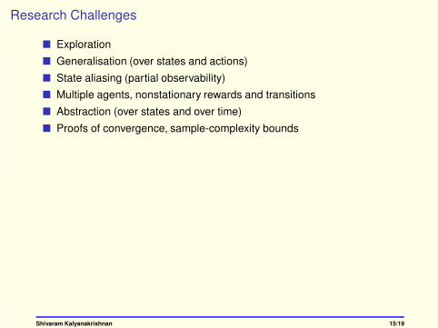
Research Challenges

� Exploration

� Generalisation (over states and actions)

� State aliasing (partial observability)

� Multiple agents, nonstationary rewards and transitions

� Abstraction (over states and over time)

� Proofs of convergence, sample-complexity bounds

Shivaram Kalyanakrishnan 15/19

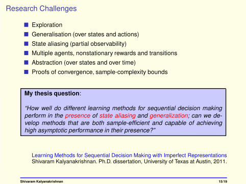
Research Challenges

� Exploration

� Generalisation (over states and actions)

� State aliasing (partial observability)

� Multiple agents, nonstationary rewards and transitions

� Abstraction (over states and over time)

� Proofs of convergence, sample-complexity bounds

My thesis question:

“How well do different learning methods for sequential decision making

perform in the presence of state aliasing and generalization; can we de-

velop methods that are both sample-efficient and capable of achieving

high asymptotic performance in their presence?”

Learning Methods for Sequential Decision Making with Imperfect RepresentationsShivaram Kalyanakrishnan. Ph.D. dissertation, University of Texas at Austin, 2011.

Shivaram Kalyanakrishnan 15/19

Practice =⇒ Imperfect Representations

TaskState State Policy RepresentationAliasing Space (Number of features)

Backgammon (T1992) Absent Discrete Neural network (198)Job-shop scheduling (ZD1995) Absent Discrete Neural network (20)Tetris (BT1906) Absent Discrete Linear (22)Elevator dispatching (CB1996) Present Continuous Neural network (46)Acrobot control (S1996) Absent Continuous Tile coding (4)Dynamic channel allocation (SB1997) Absent Discrete Linear (100’s)Active guidance of finless rocket (GM2003) Present Continuous Neural network (14)Fast quadrupedal locomotion (KS2004) Present Continuous Parameterized policy (12)Robot sensing strategy (KF2004) Present Continuous Linear (36)Helicopter control (NKJS2004) Present Continuous Neural network (10)Dynamic bipedal locomotion (TZS2004) Present Continuous Feedback control policy (2)Adaptive job routing/scheduling (WS2004) Present Discrete Tabular (4)Robot soccer keepaway (SSK2005) Present Continuous Tile coding (13)Robot obstacle negotiation (LSYSN2006) Present Continuous Linear (10)Optimized trade execution (NFK2007) Present Discrete Tabular (2-5)Blimp control (RPHB2007) Present Continuous Gaussian Process (2)9 × 9 Go (SSM2007) Absent Discrete Linear (≈1.5 million)Ms. Pac-Man (SL2007) Absent Discrete Rule list (10)Autonomic resource allocation (TJDB2007) Present Continuous Neural network (2)General game playing (FB2008) Absent Discrete Tabular (part of state space)Soccer opponent “hassling” (GRT2009) Present Continuous Neural network (9)Adaptive epilepsy treatment (GVAP2008) Present Continuous Extremely rand. trees (114)Computer memory scheduling (IMMC2008) Absent Discrete Tile coding (6)Motor skills (PS2008) Present Continuous Motor primitive coeff. (100’s)Combustion Control (HNGK2009) Present Continuous Parameterized policy (2-3)

Shivaram Kalyanakrishnan 16/19

Practice =⇒ Imperfect Representations

TaskState State Policy RepresentationAliasing Space (Number of features)

Backgammon (T1992) Absent Discrete Neural network (198)Job-shop scheduling (ZD1995) Absent Discrete Neural network (20)Tetris (BT1906) Absent Discrete Linear (22)Elevator dispatching (CB1996) Present Continuous Neural network (46)Acrobot control (S1996) Absent Continuous Tile coding (4)Dynamic channel allocation (SB1997) Absent Discrete Linear (100’s)Active guidance of finless rocket (GM2003) Present Continuous Neural network (14)Fast quadrupedal locomotion (KS2004) Present Continuous Parameterized policy (12)Robot sensing strategy (KF2004) Present Continuous Linear (36)Helicopter control (NKJS2004) Present Continuous Neural network (10)Dynamic bipedal locomotion (TZS2004) Present Continuous Feedback control policy (2)Adaptive job routing/scheduling (WS2004) Present Discrete Tabular (4)Robot soccer keepaway (SSK2005) Present Continuous Tile coding (13)Robot obstacle negotiation (LSYSN2006) Present Continuous Linear (10)Optimized trade execution (NFK2007) Present Discrete Tabular (2-5)Blimp control (RPHB2007) Present Continuous Gaussian Process (2)9 × 9 Go (SSM2007) Absent Discrete Linear (≈1.5 million)Ms. Pac-Man (SL2007) Absent Discrete Rule list (10)Autonomic resource allocation (TJDB2007) Present Continuous Neural network (2)General game playing (FB2008) Absent Discrete Tabular (part of state space)Soccer opponent “hassling” (GRT2009) Present Continuous Neural network (9)Adaptive epilepsy treatment (GVAP2008) Present Continuous Extremely rand. trees (114)Computer memory scheduling (IMMC2008) Absent Discrete Tile coding (6)Motor skills (PS2008) Present Continuous Motor primitive coeff. (100’s)Combustion Control (HNGK2009) Present Continuous Parameterized policy (2-3)

Shivaram Kalyanakrishnan 16/19

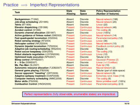
Practice =⇒ Imperfect Representations

TaskState State Policy RepresentationAliasing Space (Number of features)

Backgammon (T1992) Absent Discrete Neural network (198)Job-shop scheduling (ZD1995) Absent Discrete Neural network (20)Tetris (BT1906) Absent Discrete Linear (22)Elevator dispatching (CB1996) Present Continuous Neural network (46)Acrobot control (S1996) Absent Continuous Tile coding (4)Dynamic channel allocation (SB1997) Absent Discrete Linear (100’s)Active guidance of finless rocket (GM2003) Present Continuous Neural network (14)Fast quadrupedal locomotion (KS2004) Present Continuous Parameterized policy (12)Robot sensing strategy (KF2004) Present Continuous Linear (36)Helicopter control (NKJS2004) Present Continuous Neural network (10)Dynamic bipedal locomotion (TZS2004) Present Continuous Feedback control policy (2)Adaptive job routing/scheduling (WS2004) Present Discrete Tabular (4)Robot soccer keepaway (SSK2005) Present Continuous Tile coding (13)Robot obstacle negotiation (LSYSN2006) Present Continuous Linear (10)Optimized trade execution (NFK2007) Present Discrete Tabular (2-5)Blimp control (RPHB2007) Present Continuous Gaussian Process (2)9 × 9 Go (SSM2007) Absent Discrete Linear (≈1.5 million)Ms. Pac-Man (SL2007) Absent Discrete Rule list (10)Autonomic resource allocation (TJDB2007) Present Continuous Neural network (2)General game playing (FB2008) Absent Discrete Tabular (part of state space)Soccer opponent “hassling” (GRT2009) Present Continuous Neural network (9)Adaptive epilepsy treatment (GVAP2008) Present Continuous Extremely rand. trees (114)Computer memory scheduling (IMMC2008) Absent Discrete Tile coding (6)Motor skills (PS2008) Present Continuous Motor primitive coeff. (100’s)Combustion Control (HNGK2009) Present Continuous Parameterized policy (2-3)

Shivaram Kalyanakrishnan 16/19

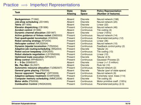
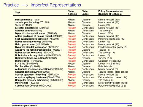
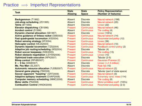
Practice =⇒ Imperfect Representations

TaskState State Policy RepresentationAliasing Space (Number of features)

Backgammon (T1992) Absent Discrete Neural network (198)Job-shop scheduling (ZD1995) Absent Discrete Neural network (20)Tetris (BT1906) Absent Discrete Linear (22)Elevator dispatching (CB1996) Present Continuous Neural network (46)Acrobot control (S1996) Absent Continuous Tile coding (4)Dynamic channel allocation (SB1997) Absent Discrete Linear (100’s)Active guidance of finless rocket (GM2003) Present Continuous Neural network (14)Fast quadrupedal locomotion (KS2004) Present Continuous Parameterized policy (12)Robot sensing strategy (KF2004) Present Continuous Linear (36)Helicopter control (NKJS2004) Present Continuous Neural network (10)Dynamic bipedal locomotion (TZS2004) Present Continuous Feedback control policy (2)Adaptive job routing/scheduling (WS2004) Present Discrete Tabular (4)Robot soccer keepaway (SSK2005) Present Continuous Tile coding (13)Robot obstacle negotiation (LSYSN2006) Present Continuous Linear (10)Optimized trade execution (NFK2007) Present Discrete Tabular (2-5)Blimp control (RPHB2007) Present Continuous Gaussian Process (2)9 × 9 Go (SSM2007) Absent Discrete Linear (≈1.5 million)Ms. Pac-Man (SL2007) Absent Discrete Rule list (10)Autonomic resource allocation (TJDB2007) Present Continuous Neural network (2)General game playing (FB2008) Absent Discrete Tabular (part of state space)Soccer opponent “hassling” (GRT2009) Present Continuous Neural network (9)Adaptive epilepsy treatment (GVAP2008) Present Continuous Extremely rand. trees (114)Computer memory scheduling (IMMC2008) Absent Discrete Tile coding (6)Motor skills (PS2008) Present Continuous Motor primitive coeff. (100’s)Combustion Control (HNGK2009) Present Continuous Parameterized policy (2-3)

Perfect representations (fully observable, enumerable states) are impractical.

Shivaram Kalyanakrishnan 16/19

Today’s Class

1. Markov decision problems

2. Bellman’s (Optimality) Equations, planning and learning

3. Challenges

4. Summary

Shivaram Kalyanakrishnan 17/19

Summary

� Learning by trial and error to perform sequential decision making.

Shivaram Kalyanakrishnan 18/19

Summary

� Learning by trial and error to perform sequential decision making.

� Given an MDP (S,A,T ,R, γ), we have to find a policy π : S → A that

yields high expected long-term reward from states.

Shivaram Kalyanakrishnan 18/19

Summary

� Learning by trial and error to perform sequential decision making.

� Given an MDP (S,A,T ,R, γ), we have to find a policy π : S → A that

yields high expected long-term reward from states.

� An optimal value function V ∗ exists, and it induces an optimal policy π∗

(several optimal policies might exist).

Shivaram Kalyanakrishnan 18/19

Summary

� Learning by trial and error to perform sequential decision making.

� Given an MDP (S,A,T ,R, γ), we have to find a policy π : S → A that

yields high expected long-term reward from states.

� An optimal value function V ∗ exists, and it induces an optimal policy π∗

(several optimal policies might exist).

� Under planning, we are given S,A,T ,R, and γ. We may compute V ∗

and π∗ using a dynamic programming algorithm such as policy iteration.

Shivaram Kalyanakrishnan 18/19

Summary

� Learning by trial and error to perform sequential decision making.

� Given an MDP (S,A,T ,R, γ), we have to find a policy π : S → A that

yields high expected long-term reward from states.

� An optimal value function V ∗ exists, and it induces an optimal policy π∗

(several optimal policies might exist).

� Under planning, we are given S,A,T ,R, and γ. We may compute V ∗

and π∗ using a dynamic programming algorithm such as policy iteration.

� In the learning context, we are given S,A, and γ: we may sample T and

R in a sequential manner. We can still converge to V ∗ and π∗ by

applying a temporal difference learning method such as Q-learning.

Shivaram Kalyanakrishnan 18/19

Summary

� Learning by trial and error to perform sequential decision making.

� Given an MDP (S,A,T ,R, γ), we have to find a policy π : S → A that

yields high expected long-term reward from states.

� An optimal value function V ∗ exists, and it induces an optimal policy π∗

(several optimal policies might exist).

� Under planning, we are given S,A,T ,R, and γ. We may compute V ∗

and π∗ using a dynamic programming algorithm such as policy iteration.

� In the learning context, we are given S,A, and γ: we may sample T and

R in a sequential manner. We can still converge to V ∗ and π∗ by

applying a temporal difference learning method such as Q-learning.

� Theory 6= Practice! In particular, convergence and optimality are difficult

to achieve when state spaces are large, and when state aliasing exists.

Shivaram Kalyanakrishnan 18/19

Summary

� Learning by trial and error to perform sequential decision making.

� Given an MDP (S,A,T ,R, γ), we have to find a policy π : S → A that

yields high expected long-term reward from states.

� An optimal value function V ∗ exists, and it induces an optimal policy π∗

(several optimal policies might exist).

� Under planning, we are given S,A,T ,R, and γ. We may compute V ∗

and π∗ using a dynamic programming algorithm such as policy iteration.

� In the learning context, we are given S,A, and γ: we may sample T and

R in a sequential manner. We can still converge to V ∗ and π∗ by

applying a temporal difference learning method such as Q-learning.

� Theory 6= Practice! In particular, convergence and optimality are difficult

to achieve when state spaces are large, and when state aliasing exists.

Thank you!

Shivaram Kalyanakrishnan 18/19

References

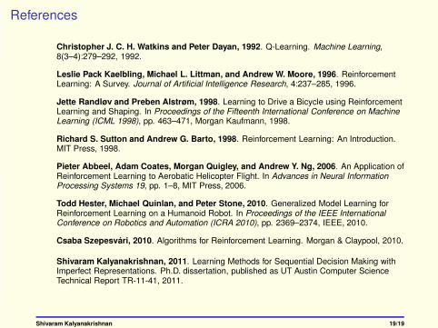
Christopher J. C. H. Watkins and Peter Dayan, 1992. Q-Learning. Machine Learning,8(3–4):279–292, 1992.

Leslie Pack Kaelbling, Michael L. Littman, and Andrew W. Moore, 1996. ReinforcementLearning: A Survey. Journal of Artificial Intelligence Research, 4:237–285, 1996.

Jette Randløv and Preben Alstrøm, 1998. Learning to Drive a Bicycle using ReinforcementLearning and Shaping. In Proceedings of the Fifteenth International Conference on MachineLearning (ICML 1998), pp. 463–471, Morgan Kaufmann, 1998.

Richard S. Sutton and Andrew G. Barto, 1998. Reinforcement Learning: An Introduction.MIT Press, 1998.

Pieter Abbeel, Adam Coates, Morgan Quigley, and Andrew Y. Ng, 2006. An Application ofReinforcement Learning to Aerobatic Helicopter Flight. In Advances in Neural InformationProcessing Systems 19, pp. 1–8, MIT Press, 2006.

Todd Hester, Michael Quinlan, and Peter Stone, 2010. Generalized Model Learning forReinforcement Learning on a Humanoid Robot. In Proceedings of the IEEE InternationalConference on Robotics and Automation (ICRA 2010), pp. 2369–2374, IEEE, 2010.

Csaba Szepesvári, 2010. Algorithms for Reinforcement Learning. Morgan & Claypool, 2010.

Shivaram Kalyanakrishnan, 2011. Learning Methods for Sequential Decision Making withImperfect Representations. Ph.D. dissertation, published as UT Austin Computer ScienceTechnical Report TR-11-41, 2011.

Shivaram Kalyanakrishnan 19/19