Ship Resistance Prediction - Verification and Validation Exercise on Unstructured Grids

VII International Conference on Computational Methods in Marine EngineeringMARINE 2017

M. Visonneau, P. Queutey and D. Le Touze (Eds)

SHIP RESISTANCE PREDICTION: VERIFICATION ANDVALIDATION EXERCISE ON UNSTRUCTURED GRIDS

P. CREPIER∗

∗Maritime Research Institute Netherlands (MARIN)P.O. Box 28

6700 AA Wageningen, The Netherlandse-mail: p.crepier@marin.nl, web page: http://www.marin.nl

Key words: CFD, KVLCC2, Verification, Validation, Double-body, Unstructured grid

Abstract. The prediction of the resistance of a ship is, together with the propeller performanceprediction, part of the key aspects during the design process of a ship, as it partly ensures thequality of the power-prediction. Body fitted structured grids for ship simulations can be ratherchallenging and time consuming to build, especially when dealing with appended ship geometries.For this reason, unstructured hexahedral trimmed grids are more and more used. Such grids canbe build by various CFD package such as CD-Adapcos Star CCM+, NUMECAs Hexpress gridgenerator or OpenFOAMSs SnappyHexMesh. Although their use is increasing or even alreadyadopted, the numerical uncertainty of these simulations seems to be a well-kept secret.

In the study presented, an attempt at quantifying the numerical uncertainty of the resistancefor the combination of the RANS Solver ReFRESCO [1] with grids generated using the com-mercial package Hexpress is made. The studied case is the flow around the bare-hull KVLCC2at model scale Reynolds number. Extensive verification and validation on the same test casehas already been published for the combination of ReFRESCO and structured grids by Pereiraet al. [2].

The method to generate grids as geometrically similar as possible is presented, and theuncertainty analysis by L. Eca and M. Hoekstra [3] is performed on the integral results obtained.The simulations are performed using the k − ω SST , k − ω TNT and the k −

√kL turbulence

models. The velocity fields calculated in the propeller plane are compared to the measured onesand to the results obtained by Pereira et al. [2] on structured grids.

The results show that the differences with the experimental results are in the same range asthe differences obtained with structured grids. The numerical uncertainties are, however, higher.They are also strongly dependent on the turbulence model used, like for structured grids, andare spread between 1.3% and 12%.

Concerning the wake flow details, not all features present in the experimental results areobtained and, compared to structured grids, the flow features are smoothed. The wake flow isalso influenced by the turbulence modelling and needs to be adressed in more detail.

1

365

P. Crepier

1 INTRODUCTION

Ship resistance predictions by means of Computational Fluid Dynamic (CFD) simulations isprogressively taking over ship model testing, especially in the early design stages of the designloop. This sort of calculations has nearly become daily routine, but the accuracy of the resultsis often overlooked. While a lot of effort is spend during workshops, like the Gothenburg orTokyo workshops, to gather validation material for various types of calm-water flows, not somuch publications about verification of the simulations performed is available. Verificationand Validation are two entirely different exercises as explained by Roache [4]: Verification isa mathematical exercise that aims at showing that we are solving the equations right, andvalidation is an engineering exercise to show that we are solving the right equations.

For ship flow simulation it is common to use body-fitted hexahedral trimmed meshes becausethey are easy to set-up even for complex geometries like appended ships. Such grids can bebuilt by most of the popular CFD software package like CD-Adapco’s Star CCM+, NUMECA’sHexpress or OpenFOAMS’s SnappyHexMesh.

L. Eca and M. Hoekstra [3] proposed a method to estimate the numerical uncertainty ofnumerical simulations based on grid refinement studies of geometrically similar grids. Generatingthe appropriate sets of grids is straightforward when using structured grids but it becomes morechallenging when working with unstructured meshes. This is most likely one of the main reasonsfor the lack of verification studies, in addition to being a rather costly exercise.

In the present study, the point of interest is the flow around the KVLCC2 at model scalefor which plenty of data is available. The grid sets are built using NUMECAs grid generatorHexpress. In section 2 a summary of the test case and in-depth details about the method used togenerate grids which are as geometrically similar as the grid generator allows. The details aboutthe RANS solver and numerical settings are provided in section 3. In section 4, the obtainedresults are detailed in terms of numerical convergence, and the uncertainty analysis is performedon the resistance components. The details of the wake flow are also shown. These results arealso compared to those obtained by Pereira et al.[2] for the same test case but with structuredgrids. Finally, in section 5, the conclusions of the findings are summarised.

2 GEOMETRY AND GRID GENERATION METHOD

2.1 KVLCC2

The object of the present study is the KVLCC2. A summary of its main particular, scaleratio and Reynolds number are provided in table 1 and a side view of the vessel is shown infigure 1.

Figure 1: Side view of the KVLCC2

2

366

P. Crepier

Table 1: Main particulars of the KVLCC2

Particular Symbol Value Unit

Length between perpendiculars Lpp 320.0 [m]

Width B 58.0 [m]

Draught T 10.8 [m]

Scale λ 58.0 [-]

Froude Number Fr 0.142 [-]

Reynolds Number Re 5.80× 106 [-]

2.2 Isotropic volume grid generation

The grids used in this study are so called trimmed meshes. In these meshes, a backgroundgrid with large cells is defined and then, the cells intersecting the input geometry are successivelydivided into 8 smaller cells to adapt to the details of the geometry. The main user input is thecell size for the initial grid, the refinement degree for each geometrical feature that should becaptured, and the size of the transition zone between two refinement levels called diffusion depthd. Once a sufficient resolution is obtained at the places of interest, an anisotropic sub-layer ofcells can be inserted to provide a grid suited to properly capture the boundary-layer on the wallspresent in the grid. The grid sets built for this study are based on an initial coarse grid whichis successively refined to obtain, in total, five grids. To obtain grids that are as geometricallysimilar as possible the following method is used:

1. The initial cell size is decreased by a factor 2, 3, 4 and 5 in each direction by using 2,3,4or 5 times more cells in each direction.

2. The surface refinement degree is kept constant throughout the sets: if, for instance, 6refinements levels are set in the initial coarse grid, the same 6 successive refinements areperformed for the other grids.

3. The size of the transition region, so-called diffusion depth d, is adapted such that it matchesthe expected final size of the grid. Details of the values used to generate the grids used inthis study are provided in section 2.4

4. The anisotropic sub-layer settings are adapted to account for the refinement performed.This step is detailed in paragraph 2.3.

Examples of the volume obtained grid after the third step are shown in figure 2 for a simplecase.

3

367

P. Crepier

(a) 2 refinement levels (b) 3 refinement levels (c) 4 refinement levels

Figure 2: Example of volume grid refinement. Black lines : initial coarse grid ; Grey lines : refined grid

2.3 Anisotropic sub-layer grid generation

The size of the cells inserted in the anisotropic sub-layer follows a geometric series of firstterm S0 ,corresponding to the first cell size, and ratio r. The size of the nth cell is then definedas follow:

Sn = S0rn (1)

With such a definition, dividing the initial cell size, and keeping the ratio constant in all gridswill not result in geometrically similar meshes. As shown in figure 3(a), when dividing the firstcell size by two and keeping the ratio constant, between 13 and 14 cells are required to obtaina distance covered by 10 cells with the initial settings instead of 20.

To obtain geometrically similar grids, both the first cell size and and ratio should be adaptedfollowing Equations 2 and 3:

Sn = S01− r

1n1

1− r1(2)

rn = r1n1 (3)

Where S0 and r1 are respectively the first cell size and growth ratio in the initial coarse grid,Sn and rn the first cell size and growth ratio for the grid refinement n, n = 1 corresponding thecoarsest grid.

Using the example in Figure 3(a) and setting up the geometric series properly, twice morecells are required with a refinement of 2 and 3 times more cells with a refinement 3, as shownin Figure 3(b).

(a) Erroneous refinement (b) Geometrically similar refinement

Figure 3: Anisotropic sub-layer refinement set-up

4

368

P. Crepier

2.4 Grid sets

Following the method described, two grid sets have been built. The sets differ only by thefirst cell size which is smaller in the second set, the isotropic volume grids are identical in bothsets. All the grids built are 6 ship lengths long (3 astern, 2 ahead) and 2 ship lengths wideand deep. The ship geometry is split in 5 different parts, aft-ship, mid-ship, bilge, fore-ship andbulbous bow, to properly set-up the surface refinements. A box of volume refinement is usedaround the whole ship to keep the grid density reasonable near the ship.

Views of the CFD domain, surfaces and boxes defined around the ship are shown in figure 4.In table 2, details of the settings used for each surface patch and the box are provided.

(a) Domain (b) Zones

Figure 4: CFD domain and definition of the surfaces and box around the ship

Table 2: Refinement levels set for each part of the grid

Part Aft-ship Mid-ship Bilge Fore-ship Bulbous Bow Box ship

Level 7 6 7 7 8 6

As detailed in section 2.2, to perform the refinement of the isotropic volume grid, only thenumber of cells in the initial grid and the transition layer are adapted. Details of the settingsused to build the 5 grids per set are detailed in table 4. The growth ratio in the anisotropicsub-layer, which starts at 1.2 in the coarsest grids, is also adapted accordingly to the refinementlevel of each grids. The number of cells obtained in each grid, as well as the average Y + obtainedwith the k − ω SST turbulence model, are presented in table 3.

3 RANS SOLVER AND NUMERICAL SETTINGS

The simulations are performed using the URANS (Unsteady Reynolds Average Navier Stokes)CFD code ReFRESCO [1]. The QUICK scheme is used for the discretisation of the convectiveflux in the momentum equations. Three different turbulence models are used in this study,namely the k−ω SST [5],k−ω TNT [6] and the k−

√kL [7]. Upwind is used for the convective

flux discretisation in the turbulence equations.

5

369

P. Crepier

Table 3: Total number of cells in each grid in million and average y+

Grid set1 2

Cell count y+2 Cell count y+2

Grid 1 0.405 0.60 0.541 0.062

Grid 2 2.79 0.30 3.826 0.030

Grid 3 8.53 0.19 11.9 0.020

Grid 4 19.1 0.14 27.1 0.015

Grid 5 35.8 0.12 51.3 0.012

Table 4: Number of cells in the three directions and diffusion depth values used for the grid sets

Grid 1 2 3 4 5

Nx 12 24 36 48 60

Ny 4 8 12 16 20

Nz 4 8 12 16 20

d 1 3 5 7 9

As boundary condition of the problem, an inflow condition is imposed at the plane upstreamof the ship and an outflow (Neumann) at the plane downstream. Symmetry conditions areimposed at the symmetry plane of the ship and at the top boundary. A constant pressure isimposed at the bottom and far-field left side of the ship. On the ship it self, a no-slip conditionis used as the grid sets built are contracted enough towards the wall such that no wall functionsare used.

4 RESULTS

4.1 NUMERICAL CONVERGENCE

In most of the simlations performed, all residuals are, on average, converged below 10−6

except for a few simulations where usually one of the turbulence quantities stagnates at a higherlevel of 10−4. This is especially true for the simulation with the k−ω based model where the ωbecomes more difficult to solve when the grid is refined.

The results show that the residuals of the continuity and momentum equations are highestaround the propeller plane while the turbulence residuals are highest at the bow of the ship.Figure 5(a) shows the convergence history of the root mean square residual for a case convergingproperly, and figure 5(b) for a stagnating case. Both figures are for the k − ω SST turbulencemodel.

6

370

P. Crepier

(a) Set 1 - Grid 5 (b) Set 2 - Grid 5

Figure 5: Convergence history for with k − ω SST

4.2 Forces uncertainty

A direct result of the simulations is the resistance of the ship. The total forces obtained andits components, pressure and friction, are normalized using equation 4:

Ci =Fi

12ρU

2∞S

(4)

Where i is the component of the force, either pressure part, friction part or total, ρ is thefluid density, U2

∞ is the free-stream velocity and S is the wetted surface of the ship.The results for the three turbulence models are gathered in table 5 for the first grid set and

in table 6 for the second one. In table 7, the experimental results as well as the results obtainedby Pereira et al. [2] for structured grids with his finest grid are listed.

For the simulations perfomed with k − ω SST , the pressure drag decreases when the grid isrefined while the friction drag increases. Both the friction and pressure drag increase when thewall resolution increases. The same behavior is obtained with k − ω TNT .

For the k −√kL, the pressure coefficient shows this similar behavior but the friction drag is

highest for the intermediate grids 2 and 3 and decreases slightly for the finest grid.When comparing the total drag, on average, all simulations underestimate the experimental

value. The maximum difference obtained with experimental drag is around 3% for k− ω TNT ,1.5% for k − ω TNT and 4% for k −

√kL.

The uncertainty analysis proposed by L. Eca and M. Hoekstra [3] has been performed in orderto quantify the discretisation error obtained with these grids. The extrapolation is performedusing only the four finest grids of each set, meaning that the grid 1 of each set is not used. Forthis reason, the uncertainty for grid 1 is not given. The obtained value is only used to show theresulting trend when using coarser grids.

7

371

P. Crepier

The obtained uncertainties are gathered in table 8 for the first grid set and in table 9 for thesecond one. For comparison, the uncertainty obtained by Pereira et al. with his finest grid aregiven at the bottom of each tables.

Table 5: Cp, Cf and Ct obtained for the first grid set

Gridk − ω SST k − ω TNT k −

√kL

Cp Cf Ct Cp Cf Ct Cp Cf Ct

Grid 1 0.78 3.22 4.00 0.77 3.33 4.09 0.80 3.25 4.05

Grid 2 0.64 3.34 3.98 0.63 3.43 4.05 0.65 3.29 3.94

Grid 3 0.62 3.37 3.99 0.61 3.47 4.07 0.62 3.29 3.91

Grid 4 0.62 3.38 4.00 0.61 3.49 4.09 0.61 3.27 3.89

Grid 5 0.63 3.38 4.01 0.62 3.49 4.11 0.61 3.27 3.88

Table 6: Cp, Cf and Ct obtained for the second grid set

Gridk − ω SST k − ω TNT k −

√kL

Cp Cf Ct Cp Cf Ct Cp Cf Ct

Grid 1 0.80 3.38 4.19 0.80 3.48 4.28 0.79 3.28 4.07

Grid 2 0.65 3.43 4.08 0.64 3.52 4.16 0.65 3.31 3.95

Grid 3 0.63 3.43 4.05 0.62 3.52 4.14 0.62 3.29 3.91

Grid 4 0.62 3.43 4.05 0.61 3.54 4.15 0.61 3.28 3.89

Grid 5 0.64 3.42 4.05 0.63 3.53 4.16 0.61 3.27 3.87

Table 7: Cp, Cf and Ct obtained by Pereira et al. and Ct obtained experimentaly (EFD)

Case Cp Cf Ct

Pereira et al. k − ω SST 0.68 3.38 4.06

Pereira et al. k − ω TNT 0.66 3.47 4.13

Pereira et al. k −√kL 0.66 3.33 3.98

EFD - - 4.11

8

372

P. Crepier

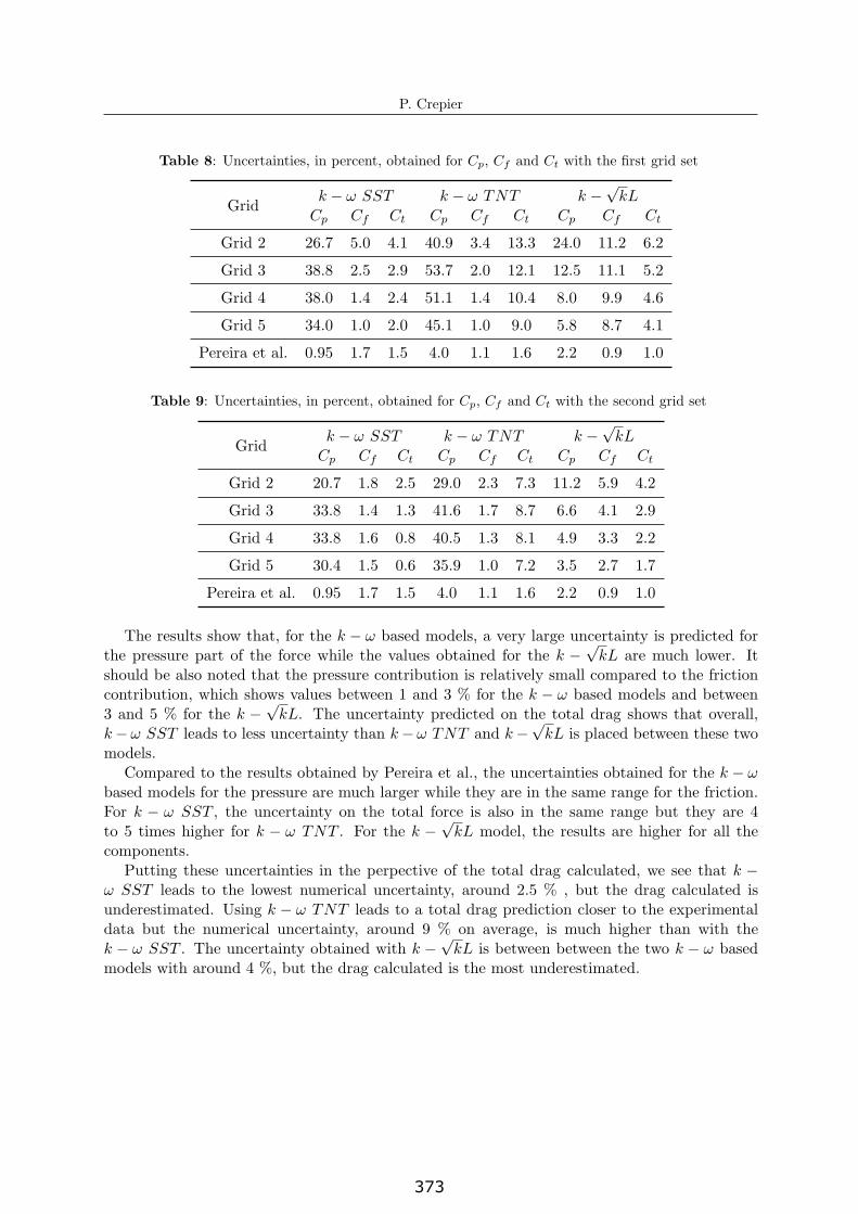
Table 8: Uncertainties, in percent, obtained for Cp, Cf and Ct with the first grid set

Gridk − ω SST k − ω TNT k −

√kL

Cp Cf Ct Cp Cf Ct Cp Cf Ct

Grid 2 26.7 5.0 4.1 40.9 3.4 13.3 24.0 11.2 6.2

Grid 3 38.8 2.5 2.9 53.7 2.0 12.1 12.5 11.1 5.2

Grid 4 38.0 1.4 2.4 51.1 1.4 10.4 8.0 9.9 4.6

Grid 5 34.0 1.0 2.0 45.1 1.0 9.0 5.8 8.7 4.1

Pereira et al. 0.95 1.7 1.5 4.0 1.1 1.6 2.2 0.9 1.0

Table 9: Uncertainties, in percent, obtained for Cp, Cf and Ct with the second grid set

Gridk − ω SST k − ω TNT k −

√kL

Cp Cf Ct Cp Cf Ct Cp Cf Ct

Grid 2 20.7 1.8 2.5 29.0 2.3 7.3 11.2 5.9 4.2

Grid 3 33.8 1.4 1.3 41.6 1.7 8.7 6.6 4.1 2.9

Grid 4 33.8 1.6 0.8 40.5 1.3 8.1 4.9 3.3 2.2

Grid 5 30.4 1.5 0.6 35.9 1.0 7.2 3.5 2.7 1.7

Pereira et al. 0.95 1.7 1.5 4.0 1.1 1.6 2.2 0.9 1.0

The results show that, for the k − ω based models, a very large uncertainty is predicted forthe pressure part of the force while the values obtained for the k −

√kL are much lower. It

should be also noted that the pressure contribution is relatively small compared to the frictioncontribution, which shows values between 1 and 3 % for the k − ω based models and between3 and 5 % for the k −

√kL. The uncertainty predicted on the total drag shows that overall,

k− ω SST leads to less uncertainty than k− ω TNT and k−√kL is placed between these two

models.Compared to the results obtained by Pereira et al., the uncertainties obtained for the k − ω

based models for the pressure are much larger while they are in the same range for the friction.For k − ω SST , the uncertainty on the total force is also in the same range but they are 4to 5 times higher for k − ω TNT . For the k −

√kL model, the results are higher for all the

components.Putting these uncertainties in the perpective of the total drag calculated, we see that k −

ω SST leads to the lowest numerical uncertainty, around 2.5 % , but the drag calculated isunderestimated. Using k − ω TNT leads to a total drag prediction closer to the experimentaldata but the numerical uncertainty, around 9 % on average, is much higher than with thek − ω SST . The uncertainty obtained with k −

√kL is between between the two k − ω based

models with around 4 %, but the drag calculated is the most underestimated.

9

373

P. Crepier

Figure 6: Experimental results obtained in the towing tank (left) and wind tunnel (right)

Figure 7: Wake flow obtained with k − ω SST with grids 3 (left) and 5 (right) from the second set

Figure 8: Results obtained by Pereira et al. with k − ω SST compared to 5th grid of second set withk − ω SST

10

374

P. Crepier

4.3 Wake flow

While the focus so far has been the verification of the integral values obtained with thesimulations, the wake flow is also a point of interest. When coupling a propeller analysis tothe resistance simulations in order to predict the power requirements of the ship, the properprediction of the wake flow is crucial.

Figure 6 shows the axial velocity contours and transverse velocity vectors obtained duringthe experiment carried out by Kim et al.[8] and Lee et al.[9] in a towing tank and windtunnelrespectively. The noticeable features of this wake flow are its hook shape and the vortex in thehook.

Figure 7 shows the obtained results with k−ω SST with grids three and five of the second set. It shows that the bilge vortex is present in the wake but the hook shape is entirely smoothed,in grid three, if not missing, in grid five. Figure 8 shows a comparison of the results obtainedby Pereira et al. with the results of this study. In the results of Pereira at al. the hook shapeis more visible but still not as pronounced as in the experimental results. Figure 8 also showsthat the boundary layer near the symmetry plane is thicker in the present study. The velocitiesfurther away of the hook shape are similar.

5 CONCLUSIONS

In this study, a method to obtain trimmed grids as geometrically similar as possible waspresented and applied to the flow around the KVLCC2 at model scale Reynold number. Twosets of five grids with different contractions towards the ship were built, and computations usingthree different turbulence models were carried out. The obtained integral results were analysedusing the method proposed by L. Eca and M. Hoekstra to estimate the discretisation errormade. The analysis shows that the numerical uncertainty decreases when using grids with ahigher contraction towards the ship.

A grid with reasonable density like Grid3, when using the k − ω SST turbulence model,results in 3% uncertainty on the total drag for the first set and 1.3% for the second set. Withk− ω TNT these values increase respectively to 12% and 8.7%. The uncertainty obtained withthe k−

√kL model are between the two k−ω based model with 5.2% with the first set and 3%

with the second set.When taking into account only the difference with the force obtained during the experiments,

the k − ω TNT model performs overall better than k − ω SST which performs better than thek −

√kL model. The k − ω TNT is on average within 1% of difference with the experimental

value, k − ω SST within 2% to 3% and k −√kL within 4% to 5%. Compared to the results

obtained by Pereira et al. for the same exercise on structured grids, the uncertainty obtainedin the present study are larger but the difference with the experiment are in the same order ofmagnitude and show the same trend.

The analysis of the velocity field in the wake of the ship shows that the grids used in thisstudy are able to capture the bilge vortex, but the hook shape visible in the axial velocity fieldis smoothed out. More details of this hook shape were captured in the results of Pereira et al.with structured grids in combination with the turbulence models used in that study, but thedeviation from the experiements are still pronounced.

The results of this study show that the numerical uncertainty and calculated drag are highly

11

375

P. Crepier

dependent on the turbulence model used. Using unstructured grids results in more uncertaintythan using structured grids even though, for the integrated values, the difference with the expri-ments are still contained in the same order of magnitude. Considering the wake flow prediction,the grids used in this study do not permit to capture the flow details at the same level as thestructured grids, but turbulence modelling also plays a major role and needs to be adressed inmore detail.

6 ACKNOWLEGEMENTS

This research is partly funded by the Dutch Ministry of Economic Affairs.

REFERENCES

[1] www.refresco.org

[2] F.S. Pereira, L. Eca. and G. Vaz. Verification and Validation Exercises for the FlowAround the KVLCC2 Tanker at Model and Full-Scale Reynolds Numbers. Ocean Engi-neering,(accepted for publication)

[3] L. Eca. and M. Hoekstra. A procedure for the estimation of the numerical uncertainty ofcfd calculations based on grid refinement studies. Journal of Computational Physics, (2014)262:104-130

[4] P. Roache. Verification of codes and calculations. AIAA Journal, 5:696-702, Vol. 36, (1998).

[5] F. R. Menter. Ten Years of Industrial Experience with the SST Turbulence Model. Turbu-lence, Heat and Mass Transfer 4, 625-632, (2003).

[6] J.C. Kok. Resolving the Dependence on Freestream Values for the k−ω Turbulence Model.American Institute of Aeronautics and Astronautics (AIAA) Journal, 38(7):1292-1295,(2000).

[7] F. R. Menter, Y. Egorov, and D. Rusch. Steady and Unsteady FlowModelling Using k−√kL

Model”. 5th International Symposium on Turbulence, Heat and Mass Transfer, (2006).

[8] W. J. Kim, S. H. Van, and D. H. Kim. Measurement of Flows Around Modern CommercialShip Models. Experiments in Fluids, 31(5):567:578, (2001).

[9] S. J. Lee, H. R. Kim, W. J. Kim and S. H. Van. Wind Tunnel Test on Flow Characteristics ofthe KRISO 3,600 TEU Containership and 300K VLCC Double-Deck Ship Models”. Journalof Ship Research, 47(1):24-38, (2003)

12

376