Shifting Ground: Landscape-Scale Modeling of ...

Environmental Management (2019) 64:416–435

https://doi.org/10.1007/s00267-019-01200-8

Shifting Ground: Landscape-Scale Modeling of BiogeochemicalProcesses under Climate Change in the Florida Everglades

Hilary Flower 1,2● Mark Rains2 ● H. Carl Fitz2,3 ● William Orem4

● Susan Newman5● Todd Z. Osborne6,7 ●

K. Ramesh Reddy7 ● Jayantha Obeysekera8

Received: 14 December 2018 / Accepted: 2 August 2019 / Published online: 22 August 2019

© Springer Science+Business Media, LLC, part of Springer Nature 2019

Abstract

Scenarios modeling can be a useful tool to plan for climate change. In this study, we help Everglades restoration planning to

bolster climate change resiliency by simulating plausible ecosystem responses to three climate change scenarios: a Baseline

scenario of 2010 climate, and two scenarios that both included 1.5 °C warming and 7% increase in evapotranspiration, and

differed only by rainfall: either increase or decrease by 10%. In conjunction with output from a water-use management

model, we used these scenarios to drive the Everglades Landscape Model to simulate changes in a suite of parameters that

include both hydrologic drivers and changes to soil pattern and process. In this paper we focus on the freshwater wetlands;

sea level rise is specifically addressed in prior work. The decreased rainfall scenario produced marked changes across the

system in comparison to the Baseline scenario. Most notably, muck fire risk was elevated for 49% of the period of simulation

in one of the three indicator regions. Surface water flow velocity slowed drastically across most of the system, which may

impair soil processes related to maintaining landscape patterning. Due to lower flow volumes, this scenario produced

decreases in parameters related to flow-loading, such as phosphorus accumulation in the soil, and methylmercury production

risk. The increased rainfall scenario was hydrologically similar to the Baseline scenario due to existing water management

rules. A key change was phosphorus accumulation in the soil, an effect of flow-loading due to higher inflow from water

control structures in this scenario.

Keywords Scenarios modeling ● Carbon ● Peat ● Phosphorus ● Sulfate ● Methylmercury

Introduction

Of all aquatic systems, wetlands are likely some of the most

susceptible to climate change, particularly those dependent

on precipitation (Burkett and Kusler 2000; Osland et al.

2016; Winter 2000). Strategies require sufficient adaptive

capacity to allow for the development of achievable goals,

the anticipation of future changes, and the overall design for

self-sustainability. This is particularly salient in the case of

the Everglades, where climate change will likely affect

precipitation and evapotranspiration, sea level, and water-

use management. Climate projections for Florida are further

complicated by the coarse grid size of existing global cir-

culation models relative to the narrow peninsular geography

that drives Florida’s climate (Obeysekera et al. 2011).

Millions of south Florida residents rely on the Everglades

for ecosystem services including supporting recreational

fisheries, providing protection from storms, and safe-

guarding drinking water from saltwater intrusion (Brown

et al. 2018; SERES 2011). As one of the largest neotropical

* Hilary Flower

[email protected]

1 Eckerd College, 4200 54th Ave S, St. Petersburg, FL 33711, USA

2 School of Geosciences, University of South Florida, 4202 E.

Fowler Ave, Tampa, FL 33620, USA

3 EcoLandMod, Inc., 1936 Harbortown Drive, Fort Pierce, FL

34946, USA

4 U.S. Geological Survey, Reston, VA 20192, USA

5 Everglades Systems Assessment Section, South Florida Water

Management District, 8894 Belvedere Road, Bldg 374, West Palm

Beach, FL 33411, USA

6 Whitney Laboratory for Marine Bioscience, University of Florida,

St. Augustine, FL 32080, USA

7 Wetland Biogeochemistry Laboratory, Soil and Water Science

Department, University of Florida, Gainesville, FL 32611, USA

8 Sea Level Solutions Center, Florida International University,

11200 SW 8th St, Miami, FL 33199, USA

1234567890();,:

1234567890();,:

http://crossmark.crossref.org/dialog/?doi=10.1007/s00267-019-01200-8&domain=pdf



http://orcid.org/0000-0002-1499-8321

http://orcid.org/0000-0002-1499-8321

http://orcid.org/0000-0002-1499-8321

http://orcid.org/0000-0002-1499-8321

http://orcid.org/0000-0002-1499-8321

mailto:[email protected]

ecoregions in North America, the Everglades also is home

to numerous rare, endangered, and threatened species,

making it a critical resource for global biodiversity. The

Everglades is an International Biosphere Reserve, a Ramsar

Wetland of International Importance, and a World Heritage

Site—one of only three places in the world given all three

distinctions (Ramsar 2019; UNESCO 2019a; UNESCO

2019b).

Unfortunately, 150 years of human impacts have

destroyed, fragmented, and degraded the ecosystem. In

2000, Congress launched the multi-billion dollar, multi-

decade Comprehensive Everglades Restoration Plan

(CERP) to restore the Everglades and to improve the ability

of the ecosystem to meet both the human and natural needs

(NRC 2016; USACE 1999). However, it is clear that the

greatest threats are yet to come, as climate change is

expected to fundamentally transform wetlands in the dec-

ades to come (Gabler et al. 2017; Osland et al. 2016),

including the Everglades (Perry 2011). For the CERP to

succeed, planners must pivot to building resiliency to these

looming threats (NRC 2016).

Scenarios modeling offers a way to envision different

plausible futures, providing a means of what-if analysis

(Moss et al. 2010). A first step is to visualize how plausible

climate scenarios may play out in the ecosystem in the

absence of restoration, with a view to identifying restoration

goals and strategies that are likely to be successful for a

range of possible outcomes. Accordingly, in 2014, the U.S.

National Research Council called for scenarios-based

modeling that provides indications of the sensitivity of the

Florida Everglades to temperature and precipitation changes

in the coming decades (NRC 2014).

The current study is the latest to follow from climate

change workshops organized by the Florida Atlantic Uni-

versity Center for Environmental Studies and the United

States Geological Survey. In 2015, researchers from the

South Florida Water Management District published cli-

mate scenarios simulations for south Florida, focusing on

providing mid-century hydrologic outcomes based on a

conservative set of climate change and sea level rise pro-

jections (Obeysekera et al. 2015). A series of what might be

called thought-experiment papers extended these hydrologic

modeling results by applying qualitative professional jud-

gements to different aspects of the Everglades ecosystem

(Aumen et al. 2015; Catano et al. 2015; Havens and

Steinman 2015; Nungesser et al. 2015; Obeysekera et al.

2015; Orem et al. 2015; van der Valk et al. 2015).

One of these papers, Orem et al. (2015), developed a

conceptual model of how climate change may affect ele-

mental cycling in Everglades soils by applying insights

from previously published studies of Everglades soils to the

hydrologic results of Obeysekera et al. (2015). In brief, they

envisioned that in a warmer but drier Everglades, large

portions of Everglades soil would undergo extended dry-

down, and loss of peat soil would be likely to exacerbate

eutrophication and contamination downstream by releasing

nutrients and contaminants such as nitrogen, phosphorus

(P), sulfur, and mercury (Orem et al. 2014). For a warmer

but wetter future, Orem et al. (2015) anticipated enhanced

peat accretion in areas that are too dry today, and a faster

flow of water that would in turn enhance the maintenance of

landscape patterning. The caveat was that increased inflow

through water structures that may accompany greater rain-

fall, may have the downside of further loading the Ever-

glades with sulfate and P, in turn exacerbating

eutrophication and methylmercury production. They con-

cluded that future changes in precipitation would be a

stronger driver of soil biogeochemical cycling than atmo-

spheric warming because of the feedbacks among water

availability, redox conditions, and organic carbon accumu-

lation in soils.

Conceptual models or frameworks are usually the first

step in any kind of modeling. A valuable next step is to

compare the conceptual assessments of future soil changes

in Orem et al. (2015) with numerical simulations by a

hydro-ecological model. The Everglades Landscape Model

(ELM) integrates a full suite of hydro-ecological processes

on a regional scale, providing the ability to model and

visualize hydro-ecological outcomes through space and

time, both at local scales (Fitz and Sklar 1999) and regional

scales (Fitz et al. 2011). The ELM has previously been used

to compare alternative restoration scenarios in the Ever-

glades (Fitz et al. 2011; Orem et al. 2014; Osborne et al.

2017). Flower et al. (2017) were the first to use the ELM to

compare how alternative climate change scenarios combine

with sea level rise to produce different effects on water

levels and salinity, vegetation dynamics, peat accretion, and

P dynamics in Everglades National Park (ENP). In the face

of sea level rise, if rainfall decreased, salinity was much

greater in the zone of saltwater encroachment, compared to

the scenario of increased rainfall. A similar amount of

freshwater marsh was lost to sea level rise in both scenarios,

but more was converted to mangroves vs. open water in the

decreased rainfall scenario compared to the increased rain-

fall scenario.

In the present paper, we provide process-based simula-

tions and visualizations that offer new insight into soil

biogeochemical outcomes under climate change scenarios.

Although the model domain includes the ENP, we focus

here on the Water Conservation Areas (WCAs) (Fig. 1). As

Flower et al. (2017) has already focused on the ENP and the

portion of our simulations that are directly affected by sea

level rise, here we focus on the freshwater remnant that will

be affected by climate change but not sea level rise. The

WCAs deserve special attention because they are spatially

and functionally central to the water management of the

Environmental Management (2019) 64:416–435 417

Everglades (Gunderson et al. 2010), and because they

contain most of the last remnants of important freshwater

habitats such as original sawgrass plain, wet prairie, and

hardwood swamps outside of ENP (Light and Dineen

1994).

Our central question is: In the coming decades, how

might soil biogeochemical processes respond to increases in

temperature, increases in evapotranspiration, and increases

or decreases in precipitation? Whereas Orem et al. (2015)

identified trajectories of change without any numerical

modeling of soil-related processes, the ELM allows us to

spatially and temporally visualize possible future trajec-

tories of nine parameters important for evaluating changes

to the soil. First, we simulate three key hydrologic drivers of

soil process and patterning: water flow volume, surface

water depth, and surface water flow velocity. Next, we look

at the effects of these drivers on soil process and patterning.

Landscape patterning will be determined by surface water

flow velocity. The amount of carbon storage as peat in the

Everglades will depend on the peat accretion rate and the

muck fire risk. Eutrophication will be determined by P

availability (driven by water inflow volume) and may be

seen most directly in the P accumulation in the soil. Sulfate

concentration in the water (also driven by water inflow

volume) will affect methylmercury production risk in

the soil.

Although model results should not be interpreted to

predict specific concentrations of chemical species at any

particular location, they do provide an overall picture of the

plausible effects of the climate model applied under dif-

ferent conditions and areas of the ecosystem most impacted

by these changes. By providing visualizations and semi-

quantitative projections of these key soil indicators, we aim

to better inform adaptive planning efforts to bolster

Everglades

Agricultural Area

Big Cypress

Na�onal

Preserve

Naples

N

Everglades

Na�onal

Park

50 km

Miami

Fort

Lauderdale

Everglades

Agricultural

Area

Florida Bay

Water

Conserva�on

Areas41

75

WCA

2A

WCA-1

2B

R. H.L.

WCA

3A North

WCA-3ASouth 3B

Lake

Okeechobee

Stormwater

Treatment Areas

Water Conserva�on Areas and

Wildlife Management Areas

Big Cypress Na�onal Preserve

Everglades Na�onal Park

Model Domain of South Florida

Water Management Model

Model Domain of Everglades

Landscape Model

Stormwater

Treatment

Areas

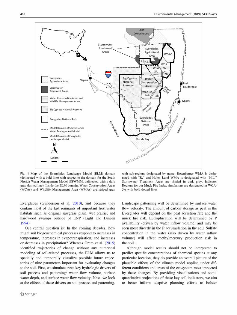
Fig. 1 Map of the Everglades Landscape Model (ELM) domain

(delineated with a bold line) with respect to the domain for the South

Florida Water Management Model (SFWMM, delineated with a dark

gray dashed line). Inside the ELM domain, Water Conservation Areas

(WCAs) and Wildlife Management Area (WMAs) are striped gray

with sub-regions designated by name; Rotenberger WMA is desig-

nated with “R.” and Holey Land WMA is designated with “H.L.”

Stormwater Treatment Areas are shaded in dark gray. Indicator

Regions for our Muck Fire Index simulations are designated in WCA-

3A with bold dotted lines

418 Environmental Management (2019) 64:416–435

Everglades resiliency to climate change and offer insights

on approaches to planners worldwide of similar wetland

ecosystems facing climate change.

Materials and Methods

Study Area

The greater Everglades of South Florida (Fig. 1) include

neotropical estuaries, wetlands, and uplands. Historically,

the abundant fresh water flowing southwesterly through the

region flowed as a sheet due to the extremely flat ground

surface extending from Lake Okeechobee to Florida Bay

and the Gulf of Mexico with an elevation gradient of only

5 cm km−1. The Everglades relies primarily on direct rain-

fall and rain-derived inflow from water control structures

(see Baseline Scenario, Table 1).

More than 50% of the historical Everglades has been lost

to agricultural and urban development (Light and Dineen

1994). The remaining Everglades wetlands have been

bisected by two main east-west trending roads, I-75

(“Alligator Alley”) and State Road 41 (“Tamiami Trail”)

(Fig. 1). Much of the remnant Everglades that lies north of

Tamiami Trail has been compartmentalized and bisected by

canals in a system of basins known as WCAs and Wildlife

Management Areas (WMAs). The northernmost of these is

WCA-1 (the Arthur R. Marshall Loxahatchee National

Wildlife Refuge), then WCA-2A and -2B to the south, with

WCA-3A adjacent to the west, WCA-3B at the southeastern

corner. South of Tamiami Trail, the ENP comprises the

remnant southern Everglades and most of Florida Bay.

Together the ENP and WCAs are designated via the Ever-

glades Forever Act (1994) the 900,000 ha (2,200,000 acres)

Everglades Protection Area (EPA). The present study

focuses on the freshwater part of the EPA. To the east of the

EPA is a densely populated urban area that includes Miami

(Fig. 1). Immediately south of Lake Okeechobee is the

Everglades Agricultural Area, a 300,000 ha (700,000 acre)

agricultural zone, which is the main source of surface water

inflow to the EPA (Abtew and Khanal 1994; Abtew and

Obeysekera 1996; Scheidt and Kalla 2007).

Surface water flow into and out of WCAs occurs through

water control structures and canals. Timing and volumes are

determined by the South Florida Water Management Dis-

trict and the Army Corps of Engineers based on multi-

objective water management decisions that balances the

needs of the EPA with the water supply demands and

protection from flooding required by the agricultural and

urban sectors. Surface water enters the ENP by passing

below Tamiami Trail from the WCAs (Fig. 1). In this study,

the main part of the ENP that we will focus on is the Shark

River Slough, which is the main flow-way which drains to

the Gulf of Mexico.

Scenarios

To extend the recent advances of prior climate-scenarios

work (Flower et al. 2017; Obeysekera et al. 2015), we used

the same Baseline scenario and scenarios of plausible future

climate change (Table 2). The period of simulation was set

for mid-21st-century (2050–2060) because Everglades

restoration commonly uses 50 years as the planning horizon

(Obeysekera et al. 2015). The CERP was approved by

congress in 2000, with projects expected to be completed in

30 years. However, restoration has been slow, and is now

estimated to take 50 years to implement.

The Baseline scenario is based on 2010 climate condi-

tions, and represents a four decade future period under

current climate conditions (Obeysekera et al. 2015). The

Table 1 Simplified water budget

for the freshwater system (i.e.,

excluding tidal exchanges)

represented as monthly means

(in millions of cubic meters) for

direct rainfall input, loss from

evapotranspiration, and water

control structure inflow

Scenario Direct

rainfall input

Loss from

evapotranspiration

Surplus (rainfall minus

evapotranspiration)

Structure inflow

Baseline 1140 977 163 228

−RF 1026 1025 1 146

+RF 1254 1109 146 252

Scenarios are existing condition (Baseline), 10% reduction (−RF), or increase (+RF) in rainfall

Table 2 Model scenarios used in

this paper, based on

precipitation, air temperature,

evapotranspiration, and sea level

rise climate change model

scenarios of Obeysekera et al.

(2015)

Scenario Precipitation Temperature Evapotranspiration Sea level rise

Baseline No change No change No change No change

−RF −10% +1.5 °C +7% +0.46 m

+RF +10% +1.5 °C +7% +0.46 m

Annual means are from the 36-year period of simulation for the Baseline and climate change scenario

simulations. Flower et al. (2017) focuses on the consequences to the Everglades of the sea level rise part of

the two climate change scenarios


Baseline scenario uses climate data from 1965 to 2000 to

capture the effects of inter-annual variability, and the two

climate change scenarios were constructed by modifying the

Baseline scenario with appropriate changes to climate and

sea level. The two climate change scenarios were derived

from a synthesis of downscaled data (Obeysekera et al.

2015; Obeysekera et al. 2011). We used projections for

2060 that are conservative for warming (1.5 °C), and sub-

sequent evapotranspiration (+7%), (Table 2) (Carter et al.

2014; Melillo et al. 2014; Obeysekera et al. 2011; SFRCCC

2015). Although the climate change scenarios included sea

level rise (0.46 m), its effect is primarily on the coastal

Everglades and was examined in a prior study (Flower et al.

2017). In this study we focus exclusively on the freshwater

remnant. The only difference in the two climate change

scenarios is whether rainfall increases or decreases by 10%;

hereafter, we refer to them simply as “+RF scenario” and

“–RF scenario,” respectively. A simple ±10% allows us to

evaluate the sensitivity of the ecosystem to alternative

rainfall outcomes in the face of increased warming and

evapotranspiration, which may be magnified if the change

exceeds 10%.

All of the scenarios for this study assume current (ca.

2012) water management infrastructure, rules, and opera-

tional criteria for flood protection, water supply or ecolo-

gical water deliveries. No CERP projects were accounted

for (Obeysekera et al. 2015).

Hydrologic Boundary Conditions

For surface water flow into and out of the ELM model

domain through control structures and canals, and for water

levels at the domain boundaries we used the hydrologic

simulations of Obeysekera et al. (2015) wherein the South

Florida Water Management Model (SFWMM) was run with

the climate scenarios from Table 2. The SFWMM is a

hydrologic model that simulates altered water level dis-

tributions and daily flows through water control structures

throughout south Florida’s urban, agricultural, and natural

systems. It uses climate input and a built-in complex

regional water management decision framework that

includes agricultural and urban water demand (Obeysekera

et al. 2015; SFWMD 2005; Tarboton et al. 1999). The

SFWMM is often referred to as the “2 × 2” model because it

uses a 2 × 2 mi (3.2 × 3.2 km) grid across the model domain

(delineated by a dark gray dashed line in Fig. 1).

Everglades Landscape Model

The ELM is a dynamic regional-scale integrated model that

simulates how changes in temperature and precipitation

may alter a complex, living system. The first publicly

released ELM version was Open Source with an extensive

documentation report (Fitz and Trimble 2006). Subsequent

improvements to the present ELM (versions 2.8 and 2.9)

were also fully documented, with the Open Source code,

data, and documentation being available at http://www.

ecolandmod.com, which should be consulted for a hierarchy

of detailed information on all aspects of the model and its

assumptions (Fitz et al. 2004; Fitz 2009; Fitz 2013; Fitz and

Paudel 2012; Fitz and Trimble 2006).

The ELM performance has been calibrated using exten-

sive field data (Fitz and Trimble 2006), and both calibration

and validation continue as new data become available.

Model calibration and validation has been conducted

mainly by comparing modeled vs. observed values at

almost 80 stations through the system. The most recent

(ELM v2.8.4; same in v2.8.6 and v2.9.0) marsh surface

water P concentrations have a median modeled vs. observed

difference of 0 μg L−1 (Fitz and Paudel 2012). Hydrologic

flow was validated using chloride as a conservative tracer,

with a median bias of 8 mg L−1 (Fitz and Trimble 2006).

The ELM soil module was largely calibrated using data

from the WCAs (Fitz and Sklar 1999; Fitz and Trimble

2006). Sulfate modeled vs. observed values (ELM v2.8.6)

differed by a median of 0 mg L−1 (Fitz 2013). Extensive

documentation reports (model structure, performance, etc)

for incremental model versions are available at http://www.

ecolandmod.com/publications/.

The ELM has been reviewed by an independent sci-

entific review panel (Mitsch et al. 2007), and has been

formally approved by the U.S. Army Corps of Engineers

for project-specific planning perspectives dealing with

water quality. Therefore, the ELM has been widely used

to evaluate changes throughout the Everglades including:

water quality and ecological outcomes from different

decompartmentalization alternative strategies in WCA-3A

(CERP 2012; Fitz et al. 2011), water sulfate and soil

methylmercury patterns that may result from alternative

approaches to Aquifer Storage and Recovery (Orem et al.

2014), and soil responses to different CERP restoration

alternatives as part of the Synthesis of Everglades

Research and Ecosystem Services (SERES) Project

(Osborne et al. 2017). Most recently the ELM was used to

consider hydro-ecological responses to climate and sea

level rise scenarios for the first time in a project focused

on ENP (Flower et al. 2017).

For this project we set a multi-decadal period of simu-

lation starting with 2015 as time zero and running for 36

years. We used the regional (10,394 km2) ELM v2.9

application at 0.25 km2 grid resolution, which is 40 times

finer resolution than the SFWMM. The model domain of

the ELM (delineated by a bold line in Fig. 1) is largely

encompassed by the SFWMM domain and includes the

EPA, the eastern part of Big Cypress National Preserve,

Rotenberger and Holey Land (HL) WMAs.


http://www.ecolandmod.com

http://www.ecolandmod.com

http://www.ecolandmod.com/publications/

http://www.ecolandmod.com/publications/

The ELM is driven by hydrologic output from the

SFWMM model, and we used SFWMM output that was

derived from the same climate scenarios we are using in

this study (Table 2). The SFWMM domain inlcudes the

ELM domain and supplies daily flow through water

management structures and canals in the ELM domain and

water levels along the ELM boundary. Within the model

domain, the ELM dynamically distributes those flows in

canals and through model grid cells, integrating surface

water/groundwater interactions, and using scenario-based

climate spatial time series input data to determine volumes

of direct rainfall input and direct output by

evapotranspiration.

The ELM fully integrates many of the components of an

ecosystem including hydrology, water quality, soils, and

macrophyte productivity and organic matter turn-over. Here

we briefly describe the hydro-ecological modules used in

this study. We emphasize that the model documentation

reports referenced above provide definitive details regarding

the model structure and performance.

Hydrologic dynamics involve a suite of modules that

involve overland, groundwater, and canal fluxes, including

their interactions. Those are relatively complex, and their

description is beyond the scope of this manuscript, but

available in the above referenced documentation and other

ELM publications referenced above. However, we note that

the overland flow velocity Performance Measure we use in

this study is simply the cumulative, net, inflow-outflow

volume flux in four grid-cell directions on a daily basis

(involving a 36-min spatial flux time step), with that flux

volume expressed as a linear flux across the 500 m grid-cell

width across the daily time period. Thus, that velocity

Performance Measure provides a grid-cell net flux velocity

at “coarse” spatio-temporal scales, but no direction (which

may be inferred by map visualization).

Phosphorus is a variable that is conserved within the

course of its transit from the surface (or porewater) column

into incorporation by live periphyton and macrophytes, with

variable stoichiometry of phosphorus:carbon ratios relative

to the pertinent community type. P limits the maximum

growth rate of the plant/periphyton communities, along with

other water and density-dependent constraints. Upon mor-

tality, P and organic matter/carbon are consolidated into

either the floc or the consolidated soil matrix.

The soil module of the ELM is encoded to include

feedbacks among hydrology, biology, and eutrophication,

with a variety of spatial trends throughout the system. The

vertical accretion of organic soil, and the carbon and P that

are thus stored, derives from the growth and mortality of

periphyton and macrophytes, both above and below-

ground, which are simulated in two other respective mod-

ules. Growth and mortality of these primary producers are

driven by a variety of factors, including water availability

and chemistry. Because the Everglades ecosystem is highly

P-limited, higher P loads generally increase plant pro-

ductivity and turnover, thereby enhancing peat accumula-

tion (Armentano et al. 2006; Gaiser et al. 2005; Osborne

et al. 2014). This is consistent with field observations from

within and without WCA-2A where cattail-infested P-enri-

ched areas were found to have three to five times higher soil

accretion rates compared to unenriched areas (Craft and

Richardson 1993).

Water availability is important to the soil module in part

because excessive water depths and excessive dry-down

periods decrease plant productivity and turnover, thereby

diminishing peat accretion. Water availability also deter-

mines the relative contribution of aerobic vs. anaerobic

decomposition rates (DeBusk and Reddy 1998) for the two

state variables for peat: the floc and the consolidated soil.

Under flooded conditions, the (slower) anaerobic rate pre-

vails. Under dry-down conditions, the aerobic rate is

applied to the unsaturated zone, and anaerobic rate is used

below that depth.

The ELM has been encoded with a Muck Fire Index is

based on a study by Smith et al. (2003), which evaluated the

risk of peat fire in the Florida Everglades based on a suite of

measurable risk factors (including surface water depth,

duration of dry-out, and water level relative to ground

surface). The ELM Muck Fire Index is measured in days,

corresponding to cumulative number of consecutive days

that the unsaturated zone extended deeper than 15 cm below

the land surface, and had unsaturated soil moisture of <50%

(Fitz et al. 2011). Because of the ephemeral nature of muck

fire risk, we chose to exhibit a time series rather than a map,

since each map would be limited to a snapshot in time or an

average for the period of simulation. Evaluating fire risk

requires “high temporal resolution” modeling, so we chose

daily data rather than monthly or an average value for the

period of simulation.

Muck fire risk also exhibits great spatial variability, and

for simple examples to demonstrate the important temporal

variability, we provide results from several regions that

represent a range from dry to wet hydrologic regimes. For

the Muck Fire Index we used a set of model grid cells

(which we refer to here as Indicator Regions) encompassing

local areas where change was considered likely due to

changes in known flow pathways. In this study, the outputs

for given Indicator Regions are provided as time series of

the daily mean values for all of the constituent cells. The

Indicator Regions are examples of dry and wet extremes

and are designated with bold dotted lines within WCA-3A

in Fig. 1: (1) a relatively dry section adjacent and parallel to

the northern boundary (21.75 km2); (2) another relatively

dry section that includes the northern part the Miami Canal

(21.25 km2); and (3) a relatively wet section that includes

the southern part of the Miami Canal.


The Sulfate Transport and Fate module incorporates a

first order, net settling rate equation, and includes sulfate

boundary conditions, a net settling rate map, and observed

data for calibrating model performance. Statistical and

graphical assessments of model performance were con-

sistent with other ELM-simulated water quality variables

(e.g. phosphorus). Details on calibration and validation can

be found in Fitz (2013) and Orem et al. (2014). Associated

with the Sulfate module is the (post-processed) empirical

relation of the (0-1) methylmercury production risk

assessment defined by Orem et al. (2014). Methylmercury

production risk is higher at sulfate concentrations that are

intermediate, rather than very high or very low. When

surface water sulfate concentrations are very low, methyl-

mercury production tends to be low, and they increase with

increasing sulfate concentrations. However, there’s a limit.

As sulfate concentrations get too high, excess sulfide (a

byproduct of sulfate reduction) begins to inhibit further

increases in methylmercury production (Orem et al. 2011).

The range of surface water sulfate concentrations that

coincide with peak methylmercury production vary

depending on wetland conditions: it is estimated to be near

10 mg/L surface water sulfate concentrations in the WCAs,

and closer to 2 mg/L in the ENP (Fitz et al. 2011).

Results

All of the simulation maps (Figs 2–4, 6, and 7) exhibit

outcomes as an average over the entire period of simulation.

Black isolines on difference maps represent approximate

confidence intervals, which vary by parameter and are based

largely upon our own expert opinion derived from devel-

opment and implementation of the ELM. Where colored

shading is visible below these isolines, interpretation should

be made with caution, because differences are small and

they may not represent real differences between the Base-

line and climate scenario runs.

Su

rfa

ce w

ate

r d

ep

th

Re

la�

ve

to

la

nd

su

rfa

ce,

cm 95

60

30

0

15

Null

Isolines

10 cm

30 cm

Baseline +RF –RF minus Baseline

Diff

ere

nce

co

mp

are

d t

o B

ase

Sce

na

rio

, cm

25

5

+RF minus Baseline

15

0

-5

-25

-15

> 25 cm< -25 cm

Black isolines at

± 5 cm

–RF minus Baseline

N

30 km

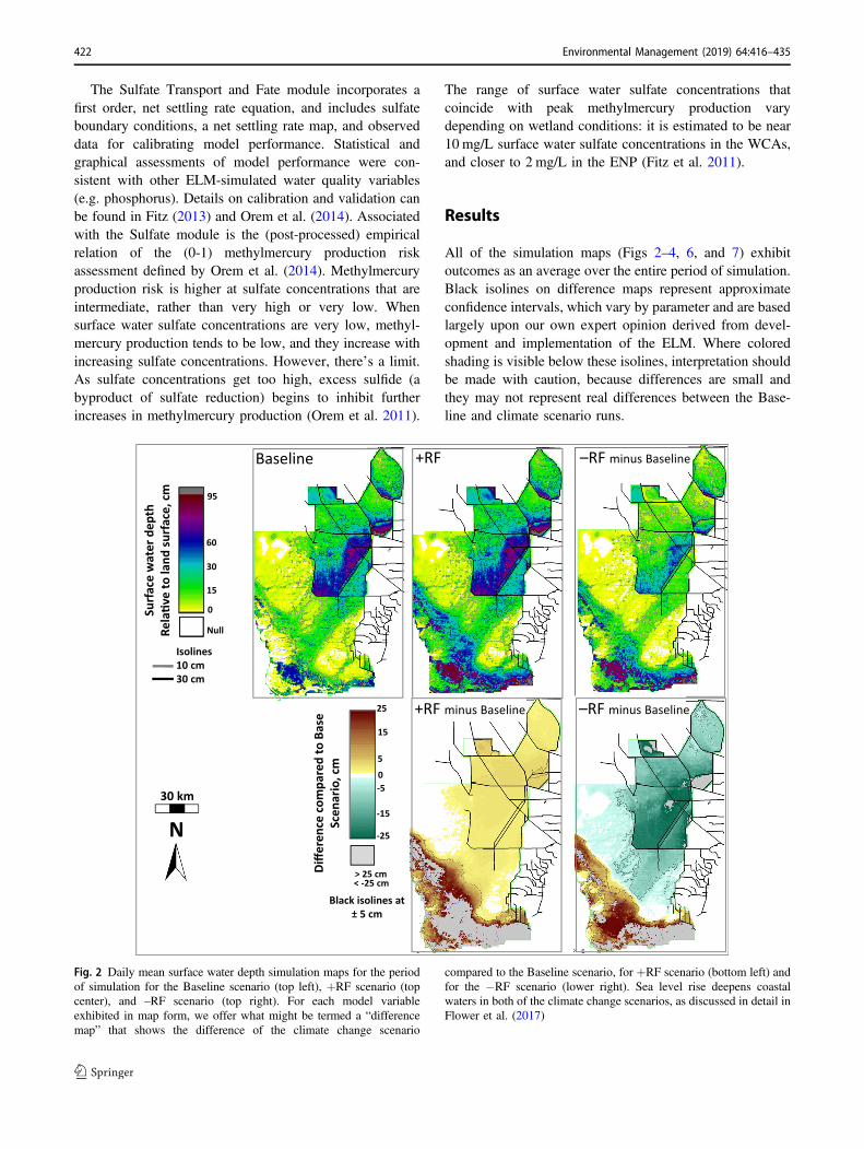
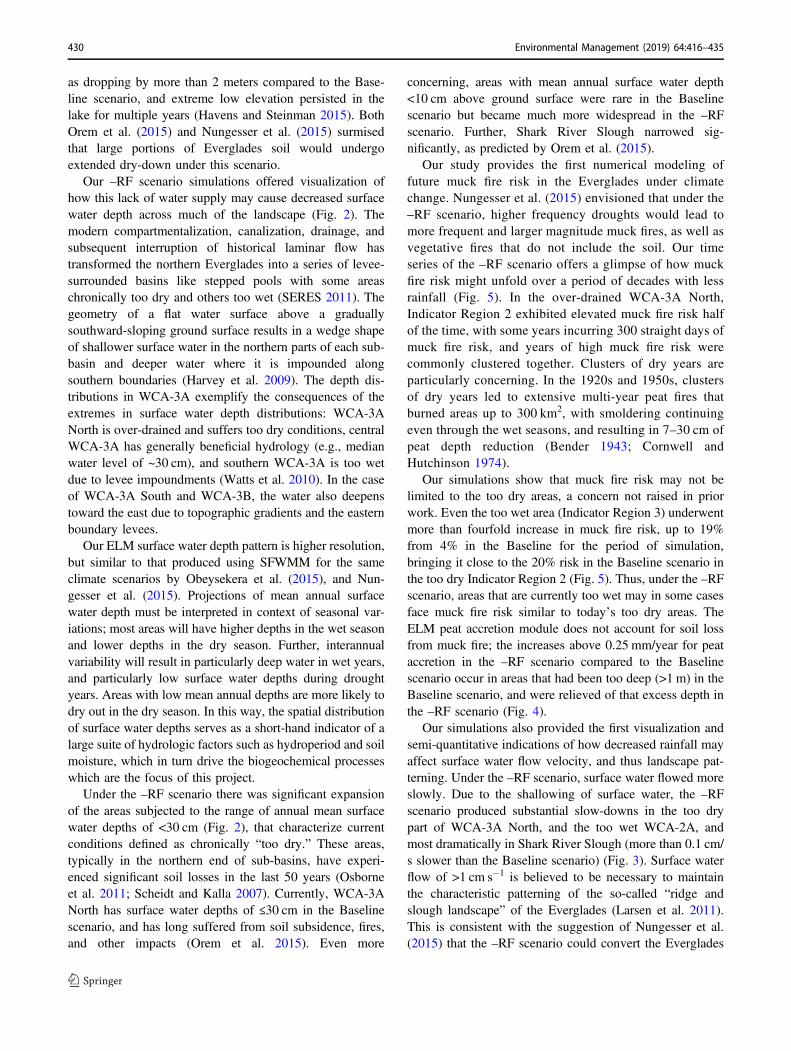
Fig. 2 Daily mean surface water depth simulation maps for the period

of simulation for the Baseline scenario (top left), +RF scenario (top

center), and –RF scenario (top right). For each model variable

exhibited in map form, we offer what might be termed a “difference

map” that shows the difference of the climate change scenario

compared to the Baseline scenario, for +RF scenario (bottom left) and

for the −RF scenario (lower right). Sea level rise deepens coastal

waters in both of the climate change scenarios, as discussed in detail in

Flower et al. (2017)


Domain-Wide Water Budgets

Baseline scenario

Direct rainfall within the model domain is high, but 85% of

it was lost to evapotranspiration, leaving a modest surplus

(rainfall minus evapotranspiration) (Table 1).

+RF scenario

The net water budget was similar to the Baseline scenario,

with a marginal increase in surplus freshwater (rainfall

minus evapotranspiration) and structural inflow. However,

the balance of water sources shifted: surplus from internal

supply (surplus) decreased by 10% compared to the surplus

in the Baseline scenario, and structural inflow increased by

about 10%.

–RF scenario

Rainfall is essentially canceled out by evapotranspiration

within the model domain, reducing surplus by 100% (Rainfall

minus Evapotranspiration is close to zero). Structural inflow

declined by 36% (from 185 to 118 million cubic meters).

Surface Water Depth Distribution

Baseline scenario

Daily mean water depth exhibited a distinctive pattern of

deepening to the south, with shallowest water in most sub-

basins in their northern section, and deepest water along its

southern boundary where the water is impounded (Fig. 2).

The shallowest water (<10 cm) was limited to a large patch in

northern WCA-1, small patches in other WCAs, and the marl

–RF+RFBaseline

Su

rfa

ce w

ate

r v

elo

city

, cm

/s 0.6

Null

0.1

Isolines

0.05 cm/s

0.1 cm/s

0.1

Diff

ere

nce

co

mp

are

d t

o

Ba

seli

ne

Sce

na

rio

, cm

/s

0

-0.1

> 0.1< -0.1

Black isolines at

± 0.05 cm/s

0.05

-0.05

+RF minus Baseline –RF minus Baseline

0.2

0.3

0.4

0.5

N

30 km

Fig. 3 Daily mean velocity of surface water flow for the period of

simulation; simulation maps for the Baseline scenario (top left), +RF

scenario (top center), and −RF scenario (top right). Difference maps

compare the +RF scenario (bottom left) and −RF scenario (lower

right) to the Baseline scenario


prairies in ENP. The north and central parts of the WCAs

exhibited relatively shallow water (<30 cm), as did the Shark

River Slough in ENP. Very deep water (>50 cm, and in some

places >100 cm) was exhibited in a large swath of WCA-3A

South, along its southern and eastern boundaries, and

throughout most of WCA-2B. In addition, all sub-basins

exhibited at least small areas of very deep water along their

southern boundaries (eastern boundary for WCA-3B).

+RF scenario

Because of (SFWMM) water management rules that attempt

to minimize excess water depths by moderating structural

inflows, surface water depths were within 5 cm of the

Baseline scenario except in two places: WCA-2B and HL

WMA where increases exceeded 5 cm.

−RF scenario

Surface water depths decreased over most of the landscape.

Depth was substantially reduced in the deeper areas by

more than 20 cm, including WCA-2B, WCA-3A South,

and HL WMA. Shallow areas underwent a smaller mag-

nitude of depth reduction, however the net effect was a

significant expansion of the total area subjected to the same

shallow surface water found drier areas today (~10–30 cm,

as found in the WCA-3A North in the Baseline scenario.

Relatively large areas appeared with mean surface water

depth <10 cm above ground surface, including northern

WCA-1, northern WCA-2A, northern WCA-3A North,

northeastern WCA-3A South, and southern and eastern HL

WMA. Shark River Slough is projected to narrow

significantly.

Velocity of Surface Water Flow

Baseline scenario

Only small isolated areas exceeded 0.5 cm/s surface water

flow rate, mainly near the southern part of the Miami Canal

in northeastern WCA-3A South (Fig. 3). Approximately

half of the northern part of the system exceeded a mean

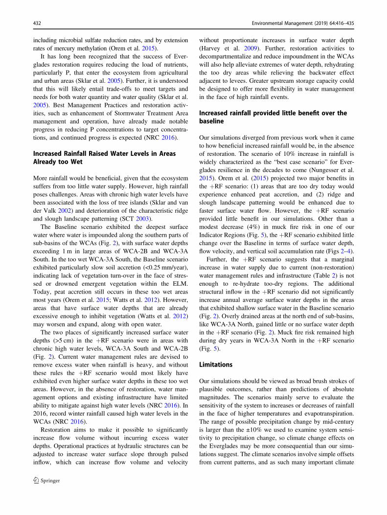
Pe

at

Acc

re�

on

Ra

te,

mm

/yr 10

5

Null

-5

-2

0

Isolines

0.25 mm/yr

2.0 mm/yr

–RF+RFBaseline

2

2.0

Diff

ere

nce

co

mp

are

d t

o B

ase

Sce

na

rio

, m

m/y

r

0.5

+RF minus Baseline1.5

0

-0.5

-2.0

-1.5

> 2 mm/yr< -2 mm/yr

Gray isolines at

± 0.25 mm/yr

Black isolines at

± 2.00 mm/yr


1.0

-1.0

N

30 km

Fig. 4 Average peat accretion rate simulation maps for the period of simulation for the Baseline scenario (top left), +RF scenario (top center), and

−RF scenario (top right). Difference maps compare the +RF scenario (bottom left) and −RF scenario (lower right) to the Baseline scenario


annual surface water flow rate of 0.1 cm/s, especially

WCA-3A North, the northern part of WCA-3A South, and

WCA-2A.

The other half of the northern Everglades exhibited a

mean annual surface water flow rate of <0.1 cm/s, including

the too wet areas of southeast WCA-3A South and WCA-

2B, as well as WCA-1 and northeastern WCA-3A North. In

the ENP, surface water flowed at 0.1-0.5 cm/s.

+RF scenario

No significant difference was exhibited compared to the

Baseline, although WCA-2A flow rates increased slightly

(<0.05 cm/s).

−RF scenario

Water flow slowed by >0.05 cm/s over large areas, parti-

cularly in WCA-3A North and most of WCA-2A, and most

dramatically in Shark River Slough (>0.1 cm/s). The –RF

scenario also accelerated surface water flow by

0.05–0.10 cm/s in some of the too wet areas of WCA-3A

South and WCA-2B, and WCA-3B.

Peat Accretion Rate

Baseline scenario

The soil accretion rate was 0.25–2 mm/year across much of

the landscape (Fig. 4). The only significant patches of little

to no soil accretion (<0.25 mm/year) were in the eastern

WCA-3A South and most of WCA-2B, which correspond

with large areas of deep surface water (Fig. 2). Faster

accretion rates (>2 mm/year) are visible across most of

WCA-2A, the perimeter of WCA-1, and at key water inflow

points in the WCAs.

+RF scenario

Soil accretion rate was nearly identical to the Baseline

scenario. Accelerated soil accretion (compared to the

Baseline scenario) only occurred in two small areas adjacent

to water inflow points (in northern WCA-2A and western

WCA-3A South).

–RF scenario

The areas that show accelerated peat accretion above the

gray isoline of 0.25 mm/year were the same places that

were also relieved of excess water depths in this scenario:

most of WCA-2A and many discrete spots in southern and

eastern WCA-3A South, as well as northern HL WMA

and much of WCA-3B. Areas adjacent to key inflow

structures, noted for faster accretion rates in the Baseline

scenario, exhibited significant changes from the Baseline

scenario. Although much of the freshwater. Everglades

shows a slight increase in peat accretion indicated by

yellow coloring, most of this is below the gray 0.25 mm/

year isoline, and thus not appreciably different from the

Baseline condition.

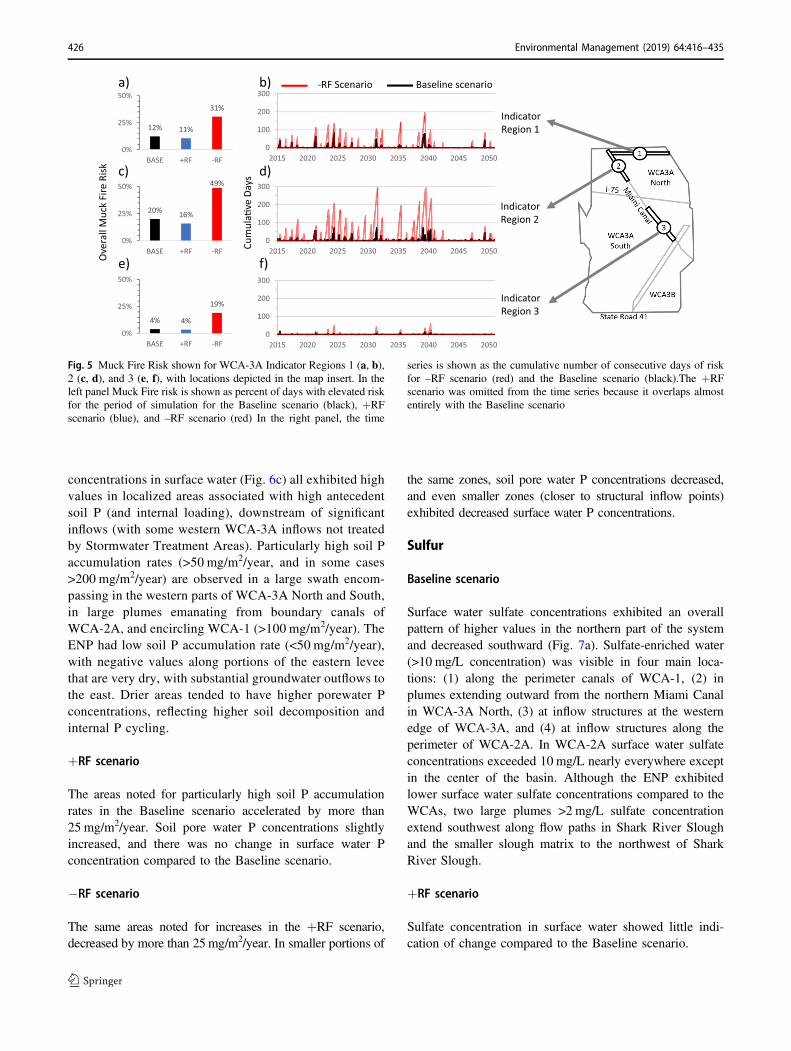
Muck Fire Risk Index

Baseline scenario

In the three multi-cell Indicator Regions we examined in

WCA-3A (Fig. 5), we found that the two locations in WCA-

3A North (which corresponded to shallow surface water in

Fig. 2) exhibited elevated muck fire risk in a relatively high

proportion of days (12 and 20% for Indicator Regions 1 and

2 respectively). The risk was very low (4%) in the deeper

part of WCA-3A South (Indicator Region 3).

+RF scenario

Muck fire risk was 4% lower than the Baseline scenario in

Indicator Region 2, the region that had the highest muck fire

risk of the three locations in the Baseline scenario. In the

other two locations, the risk was the same or slightly lower

than the Baseline scenario most of the time.

−RF scenario

Muck fire risk was more than twice as high as the

Baseline scenario in the two locations WCA-3A North,

reaching 31 and 49% of the period of simulation for

Indicator Regions 1 and 2, respectively. The northern part

of the Miami Canal (Indicator Region 2), exhibited 2

years with almost 300 days each of elevated muck fire

risk. Around 2040, a cluster of several dry years bore

little or no break from muck fire risk even during the wet

season. In the lower Miami Canal area in eastern WCA-

3A South (Indicator Region 3), which corresponds to one

of the large deep areas in Fig. 2, dry years had up to 50

consecutive days of elevated muck fire risk at a time.

Muck fire risk was elevated 19% of the time for the

period of simulation, making it similar to the region that

had the highest muck fire risk of the three locations in the

Baseline scenario.

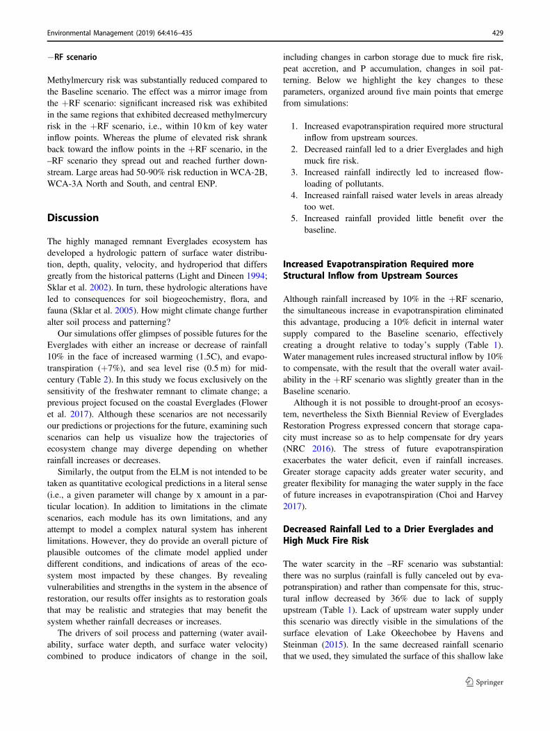
Phosphorus

Baseline scenario

Phosphorus accumulation rate in the soil (Fig. 6a), P

concentrations in soil pore water (Fig. 6b), and P


concentrations in surface water (Fig. 6c) all exhibited high

values in localized areas associated with high antecedent

soil P (and internal loading), downstream of significant

inflows (with some western WCA-3A inflows not treated

by Stormwater Treatment Areas). Particularly high soil P

accumulation rates (>50 mg/m2/year, and in some cases

>200 mg/m2/year) are observed in a large swath encom-

passing in the western parts of WCA-3A North and South,

in large plumes emanating from boundary canals of

WCA-2A, and encircling WCA-1 (>100 mg/m2/year). The

ENP had low soil P accumulation rate (<50 mg/m2/year),

with negative values along portions of the eastern levee

that are very dry, with substantial groundwater outflows to

the east. Drier areas tended to have higher porewater P

concentrations, reflecting higher soil decomposition and

internal P cycling.

+RF scenario

The areas noted for particularly high soil P accumulation

rates in the Baseline scenario accelerated by more than

25 mg/m2/year. Soil pore water P concentrations slightly

increased, and there was no change in surface water P

concentration compared to the Baseline scenario.

−RF scenario

The same areas noted for increases in the +RF scenario,

decreased by more than 25mg/m2/year. In smaller portions of

the same zones, soil pore water P concentrations decreased,

and even smaller zones (closer to structural inflow points)

exhibited decreased surface water P concentrations.

Sulfur

Baseline scenario

Surface water sulfate concentrations exhibited an overall

pattern of higher values in the northern part of the system

and decreased southward (Fig. 7a). Sulfate-enriched water

(>10 mg/L concentration) was visible in four main loca-

tions: (1) along the perimeter canals of WCA-1, (2) in

plumes extending outward from the northern Miami Canal

in WCA-3A North, (3) at inflow structures at the western

edge of WCA-3A, and (4) at inflow structures along the

perimeter of WCA-2A. In WCA-2A surface water sulfate

concentrations exceeded 10 mg/L nearly everywhere except

in the center of the basin. Although the ENP exhibited

lower surface water sulfate concentrations compared to the

WCAs, two large plumes >2 mg/L sulfate concentration

extend southwest along flow paths in Shark River Slough

and the smaller slough matrix to the northwest of Shark

River Slough.

+RF scenario

Sulfate concentration in surface water showed little indi-

cation of change compared to the Baseline scenario.

12% 11%

31%

0%

25%

50%

BASE +RF -RF

20%16%

49%

0%

25%

50%

BASE +RF -RF

4% 4%

19%

0%

25%

50%

BASE +RF -RF

-RF Scenario Baseline scenario

Indicator

Region 1

Indicator

Region 2

Indicator

Region 3

Cu

mu

la�

ve

Da

ys

Ove

rall

Mu

ck F

ire

Ris

k

0

100

200

300

2015 2020 2025 2030 2035 2040 2045 2050

0

100

200

300

2015 2020 2025 2030 2035 2040 2045 2050

0

100

200

300

2015 2020 2025 2030 2035 2040 2045 2050

a)

c)

e)

b)

d)

f)

Fig. 5 Muck Fire Risk shown for WCA-3A Indicator Regions 1 (a, b),

2 (c, d), and 3 (e, f), with locations depicted in the map insert. In the

left panel Muck Fire risk is shown as percent of days with elevated risk

for the period of simulation for the Baseline scenario (black), +RF

scenario (blue), and –RF scenario (red) In the right panel, the time

series is shown as the cumulative number of consecutive days of risk

for –RF scenario (red) and the Baseline scenario (black).The +RF

scenario was omitted from the time series because it overlaps almost

entirely with the Baseline scenario


Ph

osp

ho

rus

acc

um

ula

�o

n i

n

soil

, m

g/m

2/y

r

300

100

Null

50

-100

-50

200

0

150

Isolines

50 mg/m2/yr

100 mg/m2/yrBlack isolines at

± 10 mg/m2/yr

Baseline +RF minus Baseline –RF minus Baseline

a)

25

Diff

ere

nce

co

mp

are

d t

o

Ba

seli

ne

Sce

na

rio

, m

g/m

2/y

r

5

15

0

-5

-25

-15

> 25 mg/m2/yr

< -25 mg/m2/yr

N30 km

Baseline +RF minus Baseline

Black isolines at

± 20 µµg/L


Diff

ere

nce

co

mp

are

d t

o

Ba

seli

ne

Sce

na

rio

, µ

g/L

> 25 µg/L< -25 µg/L

25

50

0

-50

-25

Ph

osp

ho

rus

con

cen

tra

�o

n i

n

soil

po

re w

ate

r, µ

g/L

Null

250

150

200

100

0

50

Isolines

40 µg/L

100 µg/L

b)

N30 km

Ph

osp

ho

rus

con

cen

tra

�o

n

surf

ace

wa

ter,

µg

/L

50

25

Null

0

Isolines

10 µg/L

20 µg/L

Baseline 25D

iffe

ren

ce c

om

pa

red

to

Ba

seli

ne

Sce

na

rio

, µ

g/L

5

+RF minus Baseline

15

0

-5

-25

-15

> 25 µg/L< -25 µg/L

Black isolines at

± 5 µg/L


10

c)

N30 km

Fig. 6 Daily mean values for the period of simulation for a phosphorus accumulation rate in the soil, b phosphorus concentration in soil pore water,

and c phosphorus concentration in the surface water; simulation maps are provided for the Baseline scenario (maps on the left). Difference maps

compare the+ RF scenario (bottom left) and –RF scenario (lower right) to the Baseline scenario


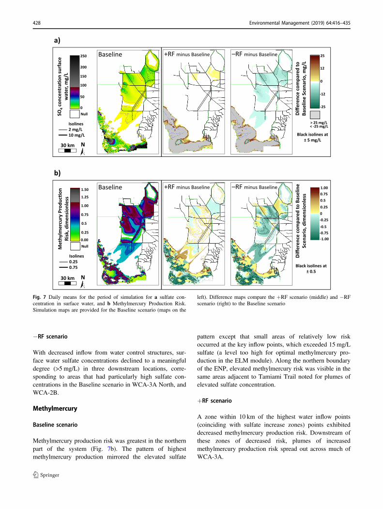
−RF scenario

With decreased inflow from water control structures, sur-

face water sulfate concentrations declined to a meaningful

degree (>5 mg/L) in three downstream locations, corre-

sponding to areas that had particularly high sulfate con-

centrations in the Baseline scenario in WCA-3A North, and

WCA-2B.

Methylmercury

Baseline scenario

Methylmercury production risk was greatest in the northern

part of the system (Fig. 7b). The pattern of highest

methylmercury production mirrored the elevated sulfate

pattern except that small areas of relatively low risk

occurred at the key inflow points, which exceeded 15 mg/L

sulfate (a level too high for optimal methylmercury pro-

duction in the ELM module). Along the northern boundary

of the ENP, elevated methylmercury risk was visible in the

same areas adjacent to Tamiami Trail noted for plumes of

elevated sulfate concentration.

+RF scenario

A zone within 10 km of the highest water inflow points

(coinciding with sulfate increase zones) points exhibited

decreased methylmercury production risk. Downstream of

these zones of decreased risk, plumes of increased

methylmercury production risk spread out across much of

WCA-3A.


Black isolines at

± 5 mg/L


a)

> 25 mg/L< -25 mg/L

12

25

0

-25

-12

250

100

0

50

200

150

Null

Isolines

2 mg/L

10 mg/L

SO

4co

nce

ntr

a�

on

su

rfa

ce

wa

ter,

mg

/L

Diff

ere

nce

co

mp

are

d t

o

Ba

seli

ne

Sce

na

rio

, m

g/L

N30 km


Black isolines at

± 0.5


b)

1.50

0.5

0.00

0.25

1.25

1.00

0.75

Null

Isolines

0.25

0.75

Me

thy

lme

rcu

ry P

rod

uc�

on

Ris

k,

dim

en

sio

nle

ss 0.5

1.00

0

-1.00

-0.5

0.25

-0.25

0.75

-0.75

Diff

ere

nce

co

mp

are

d t

o B

ase

lin

e

Sce

na

rio

, d

ime

nsi

on

less

N30 km

Fig. 7 Daily means for the period of simulation for a sulfate con-

centration in surface water, and b Methylmercury Production Risk.

Simulation maps are provided for the Baseline scenario (maps on the

left). Difference maps compare the +RF scenario (middle) and −RF

scenario (right) to the Baseline scenario


−RF scenario

Methylmercury risk was substantially reduced compared to

the Baseline scenario. The effect was a mirror image from

the +RF scenario: significant increased risk was exhibited

in the same regions that exhibited decreased methylmercury

risk in the +RF scenario, i.e., within 10 km of key water

inflow points. Whereas the plume of elevated risk shrank

back toward the inflow points in the +RF scenario, in the

–RF scenario they spread out and reached further down-

stream. Large areas had 50-90% risk reduction in WCA-2B,

WCA-3A North and South, and central ENP.

Discussion

The highly managed remnant Everglades ecosystem has

developed a hydrologic pattern of surface water distribu-

tion, depth, quality, velocity, and hydroperiod that differs

greatly from the historical patterns (Light and Dineen 1994;

Sklar et al. 2002). In turn, these hydrologic alterations have

led to consequences for soil biogeochemistry, flora, and

fauna (Sklar et al. 2005). How might climate change further

alter soil process and patterning?

Our simulations offer glimpses of possible futures for the

Everglades with either an increase or decrease of rainfall

10% in the face of increased warming (1.5C), and evapo-

transpiration (+7%), and sea level rise (0.5 m) for mid-

century (Table 2). In this study we focus exclusively on the

sensitivity of the freshwater remnant to climate change; a

previous project focused on the coastal Everglades (Flower

et al. 2017). Although these scenarios are not necessarily

our predictions or projections for the future, examining such

scenarios can help us visualize how the trajectories of

ecosystem change may diverge depending on whether

rainfall increases or decreases.

Similarly, the output from the ELM is not intended to be

taken as quantitative ecological predictions in a literal sense

(i.e., a given parameter will change by x amount in a par-

ticular location). In addition to limitations in the climate

scenarios, each module has its own limitations, and any

attempt to model a complex natural system has inherent

limitations. However, they do provide an overall picture of

plausible outcomes of the climate model applied under

different conditions, and indications of areas of the eco-

system most impacted by these changes. By revealing

vulnerabilities and strengths in the system in the absence of

restoration, our results offer insights as to restoration goals

that may be realistic and strategies that may benefit the

system whether rainfall decreases or increases.

The drivers of soil process and patterning (water avail-

ability, surface water depth, and surface water velocity)

combined to produce indicators of change in the soil,

including changes in carbon storage due to muck fire risk,

peat accretion, and P accumulation, changes in soil pat-

terning. Below we highlight the key changes to these

parameters, organized around five main points that emerge

from simulations:

1. Increased evapotranspiration required more structural

inflow from upstream sources.

2. Decreased rainfall led to a drier Everglades and high

muck fire risk.

3. Increased rainfall indirectly led to increased flow-

loading of pollutants.

4. Increased rainfall raised water levels in areas already

too wet.

5. Increased rainfall provided little benefit over the

baseline.

Increased Evapotranspiration Required moreStructural Inflow from Upstream Sources

Although rainfall increased by 10% in the +RF scenario,

the simultaneous increase in evapotranspiration eliminated

this advantage, producing a 10% deficit in internal water

supply compared to the Baseline scenario, effectively

creating a drought relative to today’s supply (Table 1).

Water management rules increased structural inflow by 10%

to compensate, with the result that the overall water avail-

ability in the +RF scenario was slightly greater than in the

Baseline scenario.

Although it is not possible to drought-proof an ecosys-

tem, nevertheless the Sixth Biennial Review of Everglades

Restoration Progress expressed concern that storage capa-

city must increase so as to help compensate for dry years

(NRC 2016). The stress of future evapotranspiration

exacerbates the water deficit, even if rainfall increases.

Greater storage capacity adds greater water security, and

greater flexibility for managing the water supply in the face

of future increases in evapotranspiration (Choi and Harvey

2017).

Decreased Rainfall Led to a Drier Everglades andHigh Muck Fire Risk

The water scarcity in the –RF scenario was substantial:

there was no surplus (rainfall is fully canceled out by eva-

potranspiration) and rather than compensate for this, struc-

tural inflow decreased by 36% due to lack of supply

upstream (Table 1). Lack of upstream water supply under

this scenario was directly visible in the simulations of the

surface elevation of Lake Okeechobee by Havens and

Steinman (2015). In the same decreased rainfall scenario

that we used, they simulated the surface of this shallow lake


as dropping by more than 2 meters compared to the Base-

line scenario, and extreme low elevation persisted in the

lake for multiple years (Havens and Steinman 2015). Both

Orem et al. (2015) and Nungesser et al. (2015) surmised

that large portions of Everglades soil would undergo

extended dry-down under this scenario.

Our –RF scenario simulations offered visualization of

how this lack of water supply may cause decreased surface

water depth across much of the landscape (Fig. 2). The

modern compartmentalization, canalization, drainage, and

subsequent interruption of historical laminar flow has

transformed the northern Everglades into a series of levee-

surrounded basins like stepped pools with some areas

chronically too dry and others too wet (SERES 2011). The

geometry of a flat water surface above a gradually

southward-sloping ground surface results in a wedge shape

of shallower surface water in the northern parts of each sub-

basin and deeper water where it is impounded along

southern boundaries (Harvey et al. 2009). The depth dis-

tributions in WCA-3A exemplify the consequences of the

extremes in surface water depth distributions: WCA-3A

North is over-drained and suffers too dry conditions, central

WCA-3A has generally beneficial hydrology (e.g., median

water level of ~30 cm), and southern WCA-3A is too wet

due to levee impoundments (Watts et al. 2010). In the case

of WCA-3A South and WCA-3B, the water also deepens

toward the east due to topographic gradients and the eastern

boundary levees.

Our ELM surface water depth pattern is higher resolution,

but similar to that produced using SFWMM for the same

climate scenarios by Obeysekera et al. (2015), and Nun-

gesser et al. (2015). Projections of mean annual surface

water depth must be interpreted in context of seasonal var-

iations; most areas will have higher depths in the wet season

and lower depths in the dry season. Further, interannual

variability will result in particularly deep water in wet years,

and particularly low surface water depths during drought

years. Areas with low mean annual depths are more likely to

dry out in the dry season. In this way, the spatial distribution

of surface water depths serves as a short-hand indicator of a

large suite of hydrologic factors such as hydroperiod and soil

moisture, which in turn drive the biogeochemical processes

which are the focus of this project.

Under the –RF scenario there was significant expansion

of the areas subjected to the range of annual mean surface

water depths of <30 cm (Fig. 2), that characterize current

conditions defined as chronically “too dry.” These areas,

typically in the northern end of sub-basins, have experi-

enced significant soil losses in the last 50 years (Osborne

et al. 2011; Scheidt and Kalla 2007). Currently, WCA-3A

North has surface water depths of ≤30 cm in the Baseline

scenario, and has long suffered from soil subsidence, fires,

and other impacts (Orem et al. 2015). Even more

concerning, areas with mean annual surface water depth

<10 cm above ground surface were rare in the Baseline

scenario but became much more widespread in the –RF

scenario. Further, Shark River Slough narrowed sig-

nificantly, as predicted by Orem et al. (2015).

Our study provides the first numerical modeling of

future muck fire risk in the Everglades under climate

change. Nungesser et al. (2015) envisioned that under the

–RF scenario, higher frequency droughts would lead to

more frequent and larger magnitude muck fires, as well as

vegetative fires that do not include the soil. Our time

series of the –RF scenario offers a glimpse of how muck

fire risk might unfold over a period of decades with less

rainfall (Fig. 5). In the over-drained WCA-3A North,

Indicator Region 2 exhibited elevated muck fire risk half

of the time, with some years incurring 300 straight days of

muck fire risk, and years of high muck fire risk were

commonly clustered together. Clusters of dry years are

particularly concerning. In the 1920s and 1950s, clusters

of dry years led to extensive multi-year peat fires that

burned areas up to 300 km2, with smoldering continuing

even through the wet seasons, and resulting in 7–30 cm of

peat depth reduction (Bender 1943; Cornwell and

Hutchinson 1974).

Our simulations show that muck fire risk may not be

limited to the too dry areas, a concern not raised in prior

work. Even the too wet area (Indicator Region 3) underwent

more than fourfold increase in muck fire risk, up to 19%

from 4% in the Baseline for the period of simulation,

bringing it close to the 20% risk in the Baseline scenario in

the too dry Indicator Region 2 (Fig. 5). Thus, under the –RF

scenario, areas that are currently too wet may in some cases

face muck fire risk similar to today’s too dry areas. The

ELM peat accretion module does not account for soil loss

from muck fire; the increases above 0.25 mm/year for peat

accretion in the –RF scenario compared to the Baseline

scenario occur in areas that had been too deep (>1 m) in the

Baseline scenario, and were relieved of that excess depth in

the –RF scenario (Fig. 4).

Our simulations also provided the first visualization and

semi-quantitative indications of how decreased rainfall may

affect surface water flow velocity, and thus landscape pat-

terning. Under the –RF scenario, surface water flowed more

slowly. Due to the shallowing of surface water, the –RF

scenario produced substantial slow-downs in the too dry

part of WCA-3A North, and the too wet WCA-2A, and

most dramatically in Shark River Slough (more than 0.1 cm/

s slower than the Baseline scenario) (Fig. 3). Surface water

flow of >1 cm s−1 is believed to be necessary to maintain

the characteristic patterning of the so-called “ridge and

slough landscape” of the Everglades (Larsen et al. 2011).

This is consistent with the suggestion of Nungesser et al.

(2015) that the –RF scenario could convert the Everglades


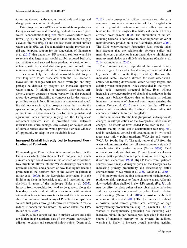
to an unpatterned landscape, as tree islands and ridge and

slough patterns continue to degrade.

Taken together, our –RF scenario simulations portray an

Everglades with internal P loading evident in elevated pore

water P concentrations (Fig. 6b), much slower surface water

flows (Fig. 3), and high rates of soil loss due to both highly

elevated fire risk (Fig. 5) and shallow mean annual surface

water depths (Fig. 2). These modeling results provide spa-

tial and temporal support for the suggestions of Nungesser

et al. (2015) that under the –RF scenario soil loss would be

so severe that large areas would exhibit exposed bedrock,

and habitats could succeed from peatland to mesic or xeric

uplands, with associated shifts in plant and animal com-

munities, including proliferation of invasive exotic species.

It seems unlikely that restoration would be able to pre-

vent long-term losses associated with the –RF scenario.

However, the changes will not occur overnight, and may

perhaps be delayed by progress on increased upstream

water storage. In addition to increased water usage effi-

ciency, greater upstream storage capacity has the potential

to provide greater flexibility to compensate for dry years by

providing extra inflow. If impacts such as elevated muck

fire risk occur rapidly, this prospect raises the risk for the

species currently relying on the Everglades. Rapid elevation

of muck fire risk also raises the risk for the large urban and

agricultural areas currently relying on the Everglades’

ecosystem services such as protection from saltwater

intrusion and storm damage. Any slowing or delayed onset

of climate-related decline would provide a critical window

of opportunity to adapt to the inevitable losses.

Increased Rainfall Indirectly Led to Increased Flow-Loading of Pollutants

Flow-loading of P and sulfate is a current problem in the

Everglades which restoration seeks to mitigate, and which

climate change could worsen in the absence of restoration.

Key structural inflows into the WCAs discharge water from

upstream sources, and a pattern of flow-loading has become

prominent in the northern part of the system in particular

(Sklar et al. 2005). In the Everglades ecosystem, P is the

limiting nutrient in bacterial, algal, and macrophyte pro-

ductivity in most of the landscape (Sklar et al. 2005).

Impacts from eutrophication tend to be greatest along the

boundary canals and at inflow structures, with nutrient

attenuation from inflow structures toward the interior mar-

shes. To minimize flow-loading of P, water from upstream

sources first passes through Stormwater Treatment Areas to

reduce P concentrations before the water enters the EPA

(Sklar et al. 2005).

Like P, sulfate concentrations in surface waters and soils

are higher in the northern part of the system, particularly

adjacent to canals and structural inflow points (Orem et al.

2011), and consequently sulfate concentrations decrease

southward. As much as one-third of the Everglades is

affected by sulfate contamination, with sulfate concentra-

tions up to 100 times higher than historical levels in heavily

affected areas (Orem 2004). The stimulation of sulfate-

reducing bacteria is considered to be an important driver of

methylmercury production in the Everglades, (Orem 2004).

The ELM Methylmercury Production Risk module takes

into account that the relationship between sulfur and

methylmercury production is non-linear, due to inhibition of

mercury methylation as sulfide levels increase (Gabriel et al.

2014; Gilmour et al. 2012).

The Baseline scenario reproduced the current pattern

wherein signs of P- and sulfate-loading are concentrated at

key water inflow points (Figs 6 and 7). Because the

increased rainfall scenario allowed for more water avail-

ability for meeting downstream water delivery targets, the

existing water management rules embedded in the hydro-

logic model increased structural inflow. Even without

increasing the concentrations of chemical constituents in the

water, mass balance dictates that an increase in volume

increases the amount of chemical constituents entering the

system. Orem et al. (2015) anticipated that the +RF sce-

nario would exacerbate the loading of these influential

chemical constituents to the Everglades.

Our simulations offer the first glimpse of landscape-scale

changes in eutrophication of the Everglades under climate

change. The effects of flow-loaded P are seen in the +RF

scenario mainly in the soil P accumulation rate (Fig. 6a),

and in accelerated vertical soil accumulation in two small

areas near inflow points (northern WCA-2A and western

WCA-3A South; Fig. 4). The rapid removal of P from the

water column means that the soil more accurately signals P

eutrophication than surface waters (Gaiser 2009). Field

observations indicate that soil P enrichment accelerates

organic matter production and processing in the Everglades

(Craft and Richardson 1993). High P loads from upstream

sources have already damaged parts of the Everglades by

increasing primary productivity and exacerbating cattail

encroachment (McCormick et al. 2002; Sklar et al. 2005).

This study provides the first simulations of methylmercury

production risk responses to future climate change. Although

flow-loaded sulfate declined in the –RF scenario (Fig. 7a), this

may be offset by short pulses of microbial sulfate reduction

and mercury methylation caused by cycles of soil oxidation

and rewetting (Orem et al. 2015), consistent with field

observations (Orem et al. 2011). The +RF scenario exhibited

a possible trend toward greater areal coverage of high

methylmercury production risk (Fig. 7b). Orem et al. (2015)

warned of methylmercury production risk increasing with

increased rainfall in part because wet deposition is the main

source of inorganic mercury to the system. In addition,

warming is likely to increase overall microbial activity,


including microbial sulfate reduction rates, and by extension

rates of mercury methylation (Orem et al. 2015).

It has long been recognized that the success of Ever-

glades restoration requires reducing the load of nutrients,

particularly P, that enter the ecosystem from agricultural

and urban areas (Sklar et al. 2005). Further, it is understood

that this will likely entail trade-offs to meet targets and

needs for both water quantity and water quality (Sklar et al.

2005). Best Management Practices and restoration activ-

ities, such as enhancement of Stormwater Treatment Area

management and operation, have already made notable

progress in reducing P concentrations to target concentra-

tions, and continued progress is expected (NRC 2016).

Increased Rainfall Raised Water Levels in AreasAlready too Wet

More rainfall would be beneficial, given that the ecosystem

suffers from too little water supply. However, high rainfall

poses challenges. Areas with chronic high water levels have

been associated with the loss of tree islands (Sklar and van

der Valk 2002) and deterioration of the characteristic ridge

and slough landscape patterning (SCT 2003).

The Baseline scenario exhibited the deepest surface

water where water is impounded along the southern parts of

sub-basins of the WCAs (Fig. 2), with surface water depths

exceeding 1 m in large areas of WCA-2B and WCA-3A

South. In the too wet WCA-3A South, the Baseline scenario

exhibited particularly slow soil accretion (<0.25 mm/year),

indicating lack of vegetation turn-over in the face of stres-

sed or drowned emergent vegetation within the ELM.

Today, peat accretion still occurs in these too wet areas

most years (Orem et al. 2015; Watts et al. 2012). However,

areas that have surface water depths that are already

excessive enough to inhibit vegetation (Watts et al. 2012)

may worsen and expand, along with open water.

The two places of significantly increased surface water

depths (>5 cm) in the +RF scenario were in areas with

chronic high water levels, WCA-3A South and WCA-2B

(Fig. 2). Current water management rules are devised to

remove excess water when rainfall is heavy, and without

these rules the +RF scenario would most likely have

exhibited even higher surface water depths in these too wet

areas. However, in the absence of restoration, water man-

agement options and existing infrastructure have limited

ability to mitigate against high water levels (NRC 2016). In

2016, record winter rainfall caused high water levels in the

WCAs (NRC 2016).

Restoration aims to make it possible to significantly

increase flow volume without incurring excess water

depths. Operational practices at hydraulic structures can be

adjusted to increase water surface slope through pulsed

inflow, which can increase flow volume and velocity

without proportionate increases in surface water depth

(Harvey et al. 2009). Further, restoration activities to

decompartmentalize and reduce impoundment in the WCAs

will also help alleviate extremes of water depth, rehydrating

the too dry areas while relieving the backwater effect

adjacent to levees. Greater upstream storage capacity could

be designed to offer more flexibility in water management

in the face of high rainfall events.

Increased rainfall provided little benefit over thebaseline

Our simulations diverged from previous work when it came

to how beneficial increased rainfall would be, in the absence

of restoration. The scenario of 10% increase in rainfall is

widely characterized as the “best case scenario” for Ever-

glades resilience in the decades to come (Nungesser et al.

2015). Orem et al. (2015) projected two major benefits in

the +RF scenario: (1) areas that are too dry today would

experience enhanced peat accretion, and (2) ridge and

slough landscape patterning would be enhanced due to

faster surface water flow. However, the +RF scenario

provided little benefit in our simulations. Other than a

modest decrease (4%) in muck fire risk in one of our

Indicator Regions (Fig. 5), the +RF scenario exhibited little

change over the Baseline in terms of surface water depth,

flow velocity, and vertical soil accumulation rate (Figs 2–4).

Further, the +RF scenario suggests that a marginal

increase in water supply due to current (non-restoration)

water management rules and infrastructure (Table 2) is not

enough to re-hydrate too-dry regions. The additional

structural inflow in the +RF scenario did not significantly

increase annual average surface water depths in the areas

that exhibited shallow surface water in the Baseline scenario

(Fig. 2). Overly drained areas at the north end of sub-basins,

like WCA-3A North, gained little or no surface water depth

in the +RF scenario (Fig. 2). Muck fire risk remained high

during dry years in WCA-3A North in the +RF scenario

(Fig. 5).

Limitations

Our simulations should be viewed as broad brush strokes of

plausible outcomes, rather than predictions of absolute

magnitudes. The scenarios mainly serve to evaluate the

sensitivity of the system to increases or decreases of rainfall

in the face of higher temperatures and evapotranspiration.

The range of possible precipitation change by mid-century

is larger than the ±10% we used to examine system sensi-

tivity to precipitation change, so climate change effects on

the Everglades may be more consequential than our simu-

lations suggest. The climate scenarios involve simple offsets

from current patterns, and as such many important climate


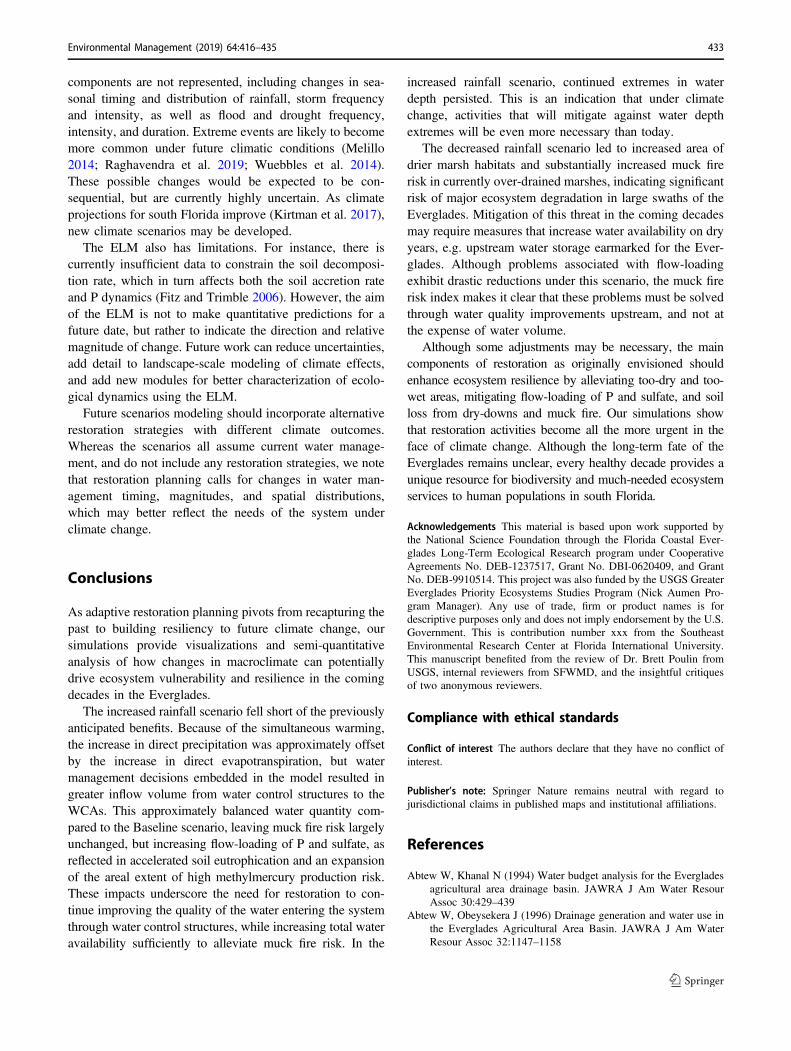
components are not represented, including changes in sea-

sonal timing and distribution of rainfall, storm frequency

and intensity, as well as flood and drought frequency,

intensity, and duration. Extreme events are likely to become

more common under future climatic conditions (Melillo

2014; Raghavendra et al. 2019; Wuebbles et al. 2014).

These possible changes would be expected to be con-

sequential, but are currently highly uncertain. As climate

projections for south Florida improve (Kirtman et al. 2017),

new climate scenarios may be developed.

The ELM also has limitations. For instance, there is

currently insufficient data to constrain the soil decomposi-

tion rate, which in turn affects both the soil accretion rate

and P dynamics (Fitz and Trimble 2006). However, the aim

of the ELM is not to make quantitative predictions for a

future date, but rather to indicate the direction and relative

magnitude of change. Future work can reduce uncertainties,

add detail to landscape-scale modeling of climate effects,

and add new modules for better characterization of ecolo-

gical dynamics using the ELM.

Future scenarios modeling should incorporate alternative

restoration strategies with different climate outcomes.

Whereas the scenarios all assume current water manage-

ment, and do not include any restoration strategies, we note

that restoration planning calls for changes in water man-

agement timing, magnitudes, and spatial distributions,

which may better reflect the needs of the system under

climate change.

Conclusions

As adaptive restoration planning pivots from recapturing the

past to building resiliency to future climate change, our

simulations provide visualizations and semi-quantitative

analysis of how changes in macroclimate can potentially

drive ecosystem vulnerability and resilience in the coming

decades in the Everglades.

The increased rainfall scenario fell short of the previously

anticipated benefits. Because of the simultaneous warming,

the increase in direct precipitation was approximately offset

by the increase in direct evapotranspiration, but water

management decisions embedded in the model resulted in

greater inflow volume from water control structures to the

WCAs. This approximately balanced water quantity com-

pared to the Baseline scenario, leaving muck fire risk largely

unchanged, but increasing flow-loading of P and sulfate, as

reflected in accelerated soil eutrophication and an expansion

of the areal extent of high methylmercury production risk.

These impacts underscore the need for restoration to con-

tinue improving the quality of the water entering the system

through water control structures, while increasing total water

availability sufficiently to alleviate muck fire risk. In the

increased rainfall scenario, continued extremes in water

depth persisted. This is an indication that under climate

change, activities that will mitigate against water depth

extremes will be even more necessary than today.

The decreased rainfall scenario led to increased area of

drier marsh habitats and substantially increased muck fire

risk in currently over-drained marshes, indicating significant

risk of major ecosystem degradation in large swaths of the

Everglades. Mitigation of this threat in the coming decades

may require measures that increase water availability on dry

years, e.g. upstream water storage earmarked for the Ever-

glades. Although problems associated with flow-loading

exhibit drastic reductions under this scenario, the muck fire

risk index makes it clear that these problems must be solved

through water quality improvements upstream, and not at

the expense of water volume.

Although some adjustments may be necessary, the main

components of restoration as originally envisioned should

enhance ecosystem resilience by alleviating too-dry and too-

wet areas, mitigating flow-loading of P and sulfate, and soil

loss from dry-downs and muck fire. Our simulations show

that restoration activities become all the more urgent in the

face of climate change. Although the long-term fate of the

Everglades remains unclear, every healthy decade provides a

unique resource for biodiversity and much-needed ecosystem

services to human populations in south Florida.

Acknowledgements This material is based upon work supported by

the National Science Foundation through the Florida Coastal Ever-

glades Long-Term Ecological Research program under Cooperative

Agreements No. DEB-1237517, Grant No. DBI-0620409, and Grant

No. DEB-9910514. This project was also funded by the USGS Greater

Everglades Priority Ecosystems Studies Program (Nick Aumen Pro-

gram Manager). Any use of trade, firm or product names is for

descriptive purposes only and does not imply endorsement by the U.S.

Government. This is contribution number xxx from the Southeast

Environmental Research Center at Florida International University.

This manuscript benefited from the review of Dr. Brett Poulin from

USGS, internal reviewers from SFWMD, and the insightful critiques

of two anonymous reviewers.

Compliance with ethical standards

Conflict of interest The authors declare that they have no conflict of

interest.

Publisher’s note: Springer Nature remains neutral with regard to

jurisdictional claims in published maps and institutional affiliations.

References

Abtew W, Khanal N (1994) Water budget analysis for the Everglades

agricultural area drainage basin. JAWRA J Am Water Resour

Assoc 30:429–439

Abtew W, Obeysekera J (1996) Drainage generation and water use in

the Everglades Agricultural Area Basin. JAWRA J Am Water

Resour Assoc 32:1147–1158


Armentano TV, Sah JP, Ross MS, Jones DT, Cooley HC, Smith CS

(2006) Rapid responses of vegetation to hydrological changes in

Taylor Slough, Everglades National Park, Florida, USA.

Hydrobiologia 569:293–309

Aumen NG, Havens KE, Best GR, Berry L (2015) Predicting ecolo-

gical responses of the Florida Everglades to possible future cli-

mate scenarios. Introd Environ Manag 55:741–748

Bender GJ. The everglades fire control district. In: soil science society

of florida. Proceedings, 1943. pp 149–152

Brown CE et al. (2018) Ecological-economic assessment of the effects

of freshwater flow in the Florida Everglades on recreational

fisheries. Sci Total Environ 627:480–493

Burkett V, Kusler J (2000) Climate change: potential impacts and

interactions in wetlands of the Untted States. JAWRA J Am

Water Resour Assoc 36:313–320

Carter LM et al. (2014) Southeast and the caribbean climate change

impacts in the United States: the third national climate assess-

ment. In: JM Melillo, Terese (TC) Richmond, GW Yohe, (eds),

U.S. Global Change Research Program, 396–417. https://doi.org/

10.7930/J0NP22CB

Catano CP et al. (2015) Using scenario planning to evaluate the

impacts of climate change on wildlife populations and commu-

nities in the Florida. Everglades Environ Manag 55:807–823

CERP (2012) CERP Decomp Water Quality Team: water conservation

area 3 decompartmentalization project implementation report 1:

everglades landscape model evaluation of water quality risk.

United States Army Corps of Engineers, Jacksonville District,

and South Florida Water Management District, West Palm Beach,

FL, and Jacksonville, FL, USA

Choi J, Harvey JW (2017) Predicting outcomes of restored Everglades

high flow: a model system for scientifically managed floodplains

Restoration Ecology 25:S39–S47

Cornwell G, Hutchinson E (1974) An ecological analysis of an Ever-

glades township in southwestern Palm Beach County, Florida. A

Report to Gulf & Western Industries and Gulf & Western Food

Products Company bu Ecoimpact Inc, Gainesville, FL, USA

Craft C, Richardson CJ (1993) Peat accretion and phosphorus accu-

mulation along a eutrophication gradient in the northern. Ever-

glades Biogeochem 22:133–156

DeBusk W, Reddy K (1998) Turnover of detrital organic carbon in a

nutrient-impacted Everglades marsh. Soil Sci Soc Am J

62:1460–1468

Fitz HC, Sklar FH, Waring T, Voinov AA, Costanza R, Maxwell T

(2004) Development and application of the Everglades Land-

scape Model. In: R Costanza and AA Voinov, editors. Landscape

Simulation Modeling: A Spatially Explicit, Dynamic Approach.

Springer Verlag, New York, pp 143–171

Fitz HC (2009) Documentation of the Everglades Landscape Model:

ELMv2.8. Ft. Lauderdale Research and Education Center, IFAS,

University of Florida, Ft. Lauderdale, FL, p 214, http://www.

ecolandmod.com/publications

Fitz HC (2013) Documentation of the Everglades Landscape Model:

ELMv2.8. 6 - Sulfate Module. Ft. Lauderdale Research and

Education Center, IFAS, University of Florida, Ft. Lauderdale,

FL, p 128, http://www.ecolandmod.com/publications

Fitz HC, Kiker GA, Kim J (2011) Integrated ecological modeling and

decision analysis within the Everglades landscape. Crit Rev

Environ Sci Technol 41:517–547

Fitz HC, Paudel R (2012) Documentation of the Everglades landscape

model: ELMv2.8. 4 Ft Lauderdale Research and Education

Center, IFAS, University of Florida, Ft Lauderdale, FL, p 364.

http://www.ecolandmod.com/publications

Fitz HC, Sklar FH (1999) Ecosystem analysis of phosphorus impacts

and altered hydrology in the Everglades: a landscape modeling

approach. In: Reddy KR, O’Connor GA, Schelske CL (eds)

Phosphorus Biogeochemistry in Subtropical Ecosystems. Lewis

Publishers, Boca Raton, FL, p 585–620

Fitz HC, Trimble B (2006) Documentation of the Everglades land-

scape model: ELM v2. 5 South Florida Water Management

District, West Palm Beach, FL

Flower H, Rains M, Fitz HC (2017) Visioning the Future: Scenarios

Modeling of the Florida Coastal Everglades. Environ Manag

60:989–1009. https://doi.org/10.1007/s00267-017-0916-2

Gabler CA et al. (2017) Macroclimatic change expected to transform

coastal wetland ecosystems this century Nature Climate Change

Gabriel MC, Howard N, Osborne TZ (2014) Fish mercury and surface

water sulfate relationships in the Everglades Protection Area.

Environ Manag 53:583–593

Gaiser E (2009) Periphyton as an indicator of restoration in the Florida

Everglades. Ecol Indic 9:S37–S45

Gaiser EE et al. (2005) Cascading ecological effects of low-level

phosphorus enrichment in the Florida Everglades. J Environ Qual

34:717–723

Gilmour C et al. (2012) Aquatic Cycling of Mercury in the Everglades:

Spatial and Temporal Trends at Ten Marsh Study Sites.

1995–2008 Final Report submitted under Contract SP689 to the

Florida Department of Environmental Protection, Tallahassee, FL

Gunderson EP, Jacobs DR, Chiang V, Lewis CE, Feng J, Quesenberry

CP, Sidney S (2010) Duration of lactation and incidence of the

metabolic syndrome in women of reproductive age according to

gestational diabetes mellitus status: a 20-Year prospective study

in CARDIA (Coronary Artery Risk Development in Young

Adults). Diabetes 59:495–504

Harvey JW, Schaffranek RW, Noe GB, Larsen LG, Nowacki DJ,

O’Connor BL (2009) Hydroecological factors governing surface

water flow on a low‐gradient floodplain Water Resources

Research 45

Havens KE, Steinman AD (2015) Ecological responses of a large

shallow lake (Okeechobee, Florida) to climate change and

potential future hydrologic regimes. Environ Manag 55:763–775

Kirtman BP, Misra V, Burgman RJ, Infanti J, Obeysekera J (2017)

Florida Climate Variability and Prediction Florida’s Climate:

Changes, Variations, & Impacts

Larsen L et al. (2011) Recent and historic drivers of landscape change

in the Everglades ridge, slough, and tree island mosaic. Critical

Reviews in Environmental Science and Technology 41:344–381

Light SS, Dineen JW (1994) Water control in the Everglades: a his-

torical perspective Everglades. Ecosyst its Restor 5:47–84

McCormick PV, Newman S, Miao S, Gawlik D, Marley D, Reddy K,

Fontaine T (2002) Effects of anthropogenic phosphorus inputs on

the Everglades The Everglades, Florida Bay, and Coral Reefs of

the Florida Keys. An Ecosystem Sourcebook CRC Press, Boca

Raton, FL, USA, p 83–126

Melillo JM (2014) Climate change impacts in the United States: the

third national climate assessment. Government Printing Office

Melillo JM, Richmond TT, Yohe G (2014) Climate change impacts in

the United States Third National Climate Assessment

Mitsch WJ, Band LE, Cerco CF (2007) Everglades Landscape Model

(ELM), Version 2.5

Moss RH et al. (2010) The next generation of scenarios for climate

change research and assessment. Nature 463:747–756

NRC (2014) National Research Council: Progress Toward Restoring

the Everglades: The Fifth Biennial Review. The National Aca-

demies Press, Washington, DC, p 302

NRC (2016) Progress Toward Restoring the Everglades: The Sixth

Biennial Review, National Research Council. The National

Academies Press, Washington, DC, 10.17226/18809

Nungesser M, Saunders C, Coronado-Molina C, Obeysekera J, John-

son J, McVoy C, Benscoter B (2015) Potential effects of climate

change on Florida’s Everglades. Environ Manag 55:824–835


https://doi.org/10.7930/J0NP22CB

https://doi.org/10.7930/J0NP22CB





https://doi.org/10.1007/s00267-017-0916-2

Obeysekera J, Barnes J, Nungesser M (2015) Climate sensitivity runs

and regional hydrologic modeling for predicting the response of

the greater Florida Everglades ecosystem to climate change.


Obeysekera J, Irizarry M, Park J, Barnes J, Dessalegne T (2011) Cli-

mate change and its implications for water resources management

in south Florida. Stoch Environ Res Risk Assess 25:495–516

Orem W, Fitz HC, Krabbenhoft D, Tate M, Gilmour C, Shafer M

(2014) Modeling sulfate transport and distribution and methyl-

mercury production associated with Aquifer Storage and

Recovery implementation in the Everglades protection area.

Sustain Water Qual Ecol 3:33–46

Orem W et al. (2011) Sulfur in the South Florida ecosystem: dis-

tribution, sources, biogeochemistry, impacts, and management for

restoration. Crit Rev Environ Sci Technol 41:249–288

Orem W, Newman S, Osborne TZ, Reddy KR (2015) Projecting

changes in Everglades soil biogeochemistry for carbon and other

key elements, to possible 2060 climate and hydrologic scenarios.


Orem WH (2004) Impacts of sulfate contamination on the Florida

Everglades ecosystem. US Department of the Interior, US Geo-

logical Survey

Osborne T, Reddy K, Ellis L, Aumen N, Surratt D, Zimmerman M,

Sadle J (2014) Evidence of recent phosphorus enrichment in

surface soils of Taylor Slough and northeast. Everglades Natl

Park Wetl 34:37–45

Osborne TZ, Fitz HC, Davis SE (2017) Restoring the foundation of the

Everglades ecosystem: assessment of edaphic responses to

hydrologic restoration scenarios. Restor Ecol 25:S59–S70

Osborne TZ et al. (2011) Landscape patterns of significant soil nutrients

and contaminants in the Greater Everglades Ecosystem: past,

present, and future. Crit Rev Environ Sci Technol 41:121–148

Osland MJ, Enwright NM, Day RH, Gabler CA, Stagg CL, Grace JB

(2016) Beyond just sea‐level rise: considering macroclimatic

drivers within coastal wetland vulnerability assessments to cli-

mate change. Glob change Biol 22:1–11

Perry J (2011) World Heritage hot spots: a global model identifies the

16 natural heritage properties on the World Heritage List most at

risk from climate change. Int J Herit Stud 17:426–441

Raghavendra A, Dai A, Milrad SM, Cloutier-Bisbee SR (2019) Flor-

idian heatwaves and extreme precipitation: future climate pro-

jections. Clim Dynam 52:495–508

Ramsar (2019) The Ramsar Convention on Wetlands: Ramsar and

World Heritage Sites. http://archive.ramsar.org/cda/en/ramsar-

documents-list-world-heritage/main/ramsar/1-31-218%5E21960_

4000_0__. Accessed 14 Jun 2019

Scheidt D, Kalla P (2007) Everglades ecosystem assessment: water

management and quality, eutrophication, mercury contamination,

soils and habitat: monitoring for adaptive management: a R-EMAP

status report. USEPA Reg 4, Athens, GA USEPA Reg. 4:98

SCT (2003) Science Coordination Team: The Role of Flow in the

Everglades Ridge and Slough Landscape. Science Coordinating

Team, South Florida Ecosystem Restoration Working Group,

Miami (FL)

SERES (2011) The Synthesis of Everglades Research and Ecosystem

Services (SERES) Project: Review of EvergladesScience, Tools,

and Needs Related to Key Science Management Questions,

p. 317. http://everglades-seres.org/SERES-_Everglades_Founda

tion/Products_files/SERES_Reviews_Merged%20copy.pdf.

Accessed 10 Jan 2018

SFRCCC (2015) South Florida Regional Climate Change Compact: a

unified sea level rise projection for Southeast Florida, Southeast

Florida Regional Climate Change Compact.

SFWMD (2005) South Florida Water Management District: Doc-

umentation of the South Florida Water Management Model

Version5.5. South Florida Water Management District, West

Palm Beach, FL

Sklar F et al. (2002) The effect of altered hydrology on the ecology of

the Everglades. In JW Porter and KG Porter, editors. The Ever-

glades, Florida bay and coral reefs of the Florida keys. An eco-

system sourcebook. CRC Press LLC, Boca Raton, FL

Sklar FH et al. (2005) The ecological-societal underpinnings of

Everglades restoration. Front Ecol Environ 3:161–169

Sklar FH, van der Valk A (2002) Tree islands of the Everglades: an

overview. In: Tree islands of the Everglades. Springer, pp. 1–18

Smith SM, Gawlik DE, Rutchey K, Crozier GE, Gray S (2003)

Assessing drought-related ecological risk in the Florida Ever-

glades. J Environ Manag 68:355–366

Tarboton K, Neidrauer C, Santee E, Needle J (1999) Regional

hydrologic modeling for planning the management of South

Florida’s water resources through 2050 American Society of

Agricultural Engineers Paper Number 992062

UNESCO (2019a) United Nations Educational, Scientific, and Cultural

Organization: Europe & North America: 292 Biosphere Reserves

in 37 Countries. http://www.unesco.org/new/en/natural-sciences/

environment/ecological-sciences/biosphere-reserves/europe-

north-america/. Accessed 14 Jun 2019

UNESCO (2019b) United Nations Educational, Scientific, and Cul-

tural Organization: World Heritage List. http://whc.unesco.org/

en/list/. Accessed 14 Jun 2019

USACE (1999) U.S. Army Corps of Engineers and South Florida

Water Management District: The Central and Southern Florida

Flood Control Project Comprehensive Review Study Final Inte-

grated Feasibility Report and Programmatic Environmental

Impact Statement (PEIS).

van der Valk AG, Volin JC, Wetzel PR (2015) Predicted changes in

interannual water-level fluctuations due to climate change and its

implications for the vegetation of the Florida Everglades. Environ

Manag 55:799–806

Watts AC, Kobziar LN, Snyder JR (2012) Fire reinforces structure of

pondcypress (Taxodium distichum var. imbricarium) domes in a

wetland landscape. Wetlands 32:439–448

Watts DL, Cohen MJ, Heffernan JB, Osborne TZ (2010) Hydrologic

modification and the loss of self-organized patterning in the

ridge–slough mosaic of the Everglades. Ecosystems

13:813–827

Winter TC (2000) The vulnerability of wetlands to climate change: a

hydrologic landscape perspective. JAWRA J Am Water Resour

Assoc 36:305–311

Wuebbles D et al. (2014) CMIP5 climate model analyses: climate

extremes in the United States. Bull Am Meteorol Soc

95:571–583


http://archive.ramsar.org/cda/en/ramsar-documents-list-world-heritage/main/ramsar/1-31-218%5E21960_4000_0__



http://everglades-seres.org/SERES-_Everglades_Foundation/Products_files/SERES_Reviews_Merged%20copy.pdf

http://everglades-seres.org/SERES-_Everglades_Foundation/Products_files/SERES_Reviews_Merged%20copy.pdf

http://www.unesco.org/new/en/natural-sciences/environment/ecological-sciences/biosphere-reserves/europe-north-america/



http://whc.unesco.org/en/list/

http://whc.unesco.org/en/list/

Shifting Ground: Landscape-Scale Modeling of ...

Documents

Transcript of Shifting Ground: Landscape-Scale Modeling of ...