Institute for International Integration Studies

IIIS Discussion Paper

No.176 / September 2006

Shift versus traditional contagion in Asian markets

Thomas FlavinNational University of Ireland, Maynooth

Ekaterini PanopoulouNational University of Ireland, Maynooth

IIIS Discussion Paper No. 176

Shift versus traditional contagion in Asian markets Thomas Flavin

Ekaterini Panopoulou

Disclaimer Any opinions expressed here are those of the author(s) and not those of the IIIS. All works posted here are owned and copyrighted by the author(s). Papers may only be downloaded for personal use only.

Shift versus traditional contagion in Asian markets

Thomas Flavin∗ Ekaterini Panopoulou National University of Ireland, Maynooth

September 2006

Abstract

We test for shift contagion between pairs of East Asian equity markets over a sample including the financial crisis of the 1990’s. Employing the methodology of Gravelle et al. (2006), we find little evidence of change in the mechanism by which common shocks are transmitted between countries. Furthermore, we analyze the effects of idiosyncratic shocks and generate time-varying conditional correlations. While there clearly is significant time variation in the pair wise correlations, this is not more pronounced during the Asian crisis than it had been historically. Keywords: Shift contagion; Financial market crises; Regime switching; Structural transmission; Emerging markets JEL Classification: F42; G15; C32

∗ Correspondence to: Thomas Flavin, Department of Economics, NUI Maynooth, Maynooth, Co. Kildare, Ireland. Tel: + 353 1 7083369, Fax: + 353 1 7083934, Email: thomas.flavin@nuim.ie

1. Separate Title Page

1

1. Introduction

A major crisis swept through many Asian financial markets in the late 1990s.

The entire financial system was rocked by adverse shocks, which spread throughout

the region and affected currency, equity and fixed income markets alike. In its

aftermath, both policy makers and financial market participants became embroiled in

a debate as to whether or not this episode represented market contagion. The extent

to which financial crises are contagious and how this contagion can be reduced or

eliminated represents a major difficulty for all market agents.

Despite the voluminous literature generated during this and earlier debates

following the US market crash of 1987, there is still little consensus as to what exactly

is meant by contagion. The academic literature tends to distinguish between

‘fundamentals based’ and ‘pure’ contagion. The former occurs due to pre-existing

market linkages such as goods trade, financial flows and other economic

connections. It occurs due to common factors. The latter reflects excess contagion

suffered during a crisis that is not explained by market fundamentals. Such

contagion is due to country-specific shocks. 1 It is important to correctly identify the

type of contagion that is present in markets before prescribing policy to deal with it.

For example, if markets decline due to ‘pure’ contagion, then policies such as capital

controls aimed at breaking market linkages are unlikely to be successful. A better

strategy would be to introduce policies aimed at reducing country specific risks.

Whether or not the crisis period was characterized by contagion in East Asian

equity markets has already attracted much attention but there is great disparity in

the reported results. For example, Forbes and Rigobon (2002) reject the hypothesis

that correlation coefficients between markets increased significantly during the crisis

period, while Rigobon (2003b) fails to find evidence of a structural break in the

propagation of shocks. Likewise, Bordo and Mucshid (2000) fail to find evidence in

favor of contagion during this crisis. In contrast, Corsetti et al (2001), Caporale et al.

(2003), Bekaert et al. (2005), and Bond et al. (2006) all find evidence of contagion

between many pairs of Asian markets.2

1 For an overview of the various definitions of contagion, the reader is referred to Dornbusch et al. (2000) or Pericoli and Sbracia (2003). 2 For a more complete review of the literature, the reader is referred to Dungey et al. (2006) and references therein.

* 3. Blinded Manuscript

2

Once more, we focus on the equity markets of this region. We choose equity

markets since a comparison of results from Dungey et al. (2003, 2004) suggests that

the impact of contagion on return variation is more important for equity rather than

currency markets. In this study, we specifically test for the presence of changes in the

transmission mechanism of common shocks between pairs of countries. The

phenomenon has been termed ‘shift’ contagion in the literature. In essence, it states

that in the absence of contagious effects, common shocks should be transmitted in

the same manner during both ‘normal’ and ‘crises’ periods. Hence, we aim to

disentangle changes in the structural transmission mechanism of shocks from

changes in the volatility due to increased common volatility shocks. We employ the

methodology of Gravelle et al. (2006, henceforth GKM) to test if the process

governing the transmission of common shocks changed during the turbulent period

associated with the Asian crisis. GKM specify a bivariate regime-switching model in

which both common and idiosyncratic shocks move between low- and high-volatility

episodes. 3 This provides (as discussed below) an unambiguous test of structural

changes in asset return co-movements between regimes.

This method has many advantages over and above previous techniques.

Firstly, the country where the shock originated does not need to be identified or

included in the analysis. Hence we can focus on the Asian markets and detect

changes in the transmission of shocks that may have originated elsewhere. This is

going to be particularly beneficial in the latter part of our sample when the LTCM

and Russian crisis occurred. Of course, the source of the shock may itself be a

disputed issue. In the extant literature, Forbes and Rigobon (2002) and Bond et al.

(2005) identify Hong Kong as the source of the crisis, while Thailand is identified as

the source in Kleimeier et al. (2003) and Baur and Schulze (2005). Secondly, the start

and end points of the high-volatility regime are determined by the data and do not

have to be exogenously specified as in Forbes and Rigobon (2002). The exogenous

choice of crisis period is often a contentious issue (see Kaminsky and Schmukler,

1999) and may be further compounded by having more than one shock

simultaneously impacting on equity markets. Rigobon (2003a) stresses the

importance of correctly specifying the crisis period. Thirdly, the test for shift

contagion is akin to testing for contagion transmitted through common fundamentals

3 Regime-switching models have been shown to perform well in capturing equity market behaviour, e.g Ang and Bekaert (2002) and Guidolin and Timmermann (2005).

3

but has the added advantage that we do not have to explicitly identify these factors.4

Simultaneously, we allow the common and idiosyncratic shocks to be regime

switching, which facilitates comparison of their relative importance in generating

movements in the estimated conditional correlations.

Our paper is organized as follows. Section 2 presents our model. Section 3

describes the data and presents our empirical findings and the tests for contagion. It

proceeds to examine the ‘traditional’ view of contagion. Section 4 investigates the

impact of foreign exchange risk on our results and also serves as a robustness check.

Section 5 summarizes our empirical findings and offers some policy implications.

2. Econometric Methodology

In this section, we present the empirical model employed to study the

interdependence between two stock markets during both calm and turbulent

periods. Let tr1 and tr2 represent stock market returns from countries 1 and 2,

respectively. These can be decomposed into an expected component, ,iµ and an

unexpected one, itu , reflecting unexpected information becoming available to

investors, i.e.

.0),( and 2,1,0)(, 21 ≠==+= ttititiit uuEiuEur µ (1)

The existence of contemporaneous correlation between the forecast errors

tt uu 21 and suggests that common structural shocks are driving both returns.

Therefore, we decompose the forecast errors into two structural shocks, one

idiosyncratic and one common. Let 2,1, and =izz itct denote the common and

idiosyncratic common shocks respectively and let the impacts of these shocks on

asset returns be 2,1, and =iitcit σσ . Then the forecast errors are written as:

.2,1, =+= izzu ititctcitit σσ (2)

Normalizing the variance of shocks to unity implies that the impact coefficients may

be interpreted as the standard deviations of structural shocks.

Following GKM we allow both the common and the idiosyncratic shocks to

switch between two states – high- and low-volatility.5 Thus, the structural impact

4 Prescribing appropriate fundamental factors in another contentious issue for Asian economies; see Karolyi (2003) and Dungey et al. (2006). 5 This heterogeneity in the heteroskedasticity of the structural shocks ensures the identification of the system (see also Rigobon, 2003a). As argued by GKM, only the assumption of regime switching in the common shocks is necessary for this. For further

4

coefficients 2,1,, =ictit σσ are given by the following:

2,1 ,)1(

2,1 ,)1(

=+−=

=+−=∗

∗

iSS

iSS

ctcictcicit

itiitiit

σσσ

σσσ (3)

where ciSit ,2,1),1,0( == are state variables that take the value of zero in normal

and unity in turbulent times. Variables with an asterisk belong to the high-volatility

or crisis regime. To complete the model, we need to specify the evolution of regimes

over time. Following the regime-switching literature, the regime paths are Markov

switching and consequently are endogenously determined. Specifically, the

conditional probabilities of remaining in the same state, i.e. not changing regime are

defined as follows:

cipSSciqSS

iitit

iitit,2,1,]1/1[Pr,2,1,]0/0[Pr

========

(4)

Furthermore, we relax the assumption of expected constant returns in (1).

These are allowed to be time varying and depend on the state of the common shock.6

In this respect, our model suggests that part of the stock market return represents a

risk premium that changes with the level of volatility.7 In particular, expected returns

are modeled as follows:

2,1 ,)1( =+−= ∗ iSS ctictiit µµµ (5)

Given that idiosyncratic shocks are uncorrelated with common shocks and mainly

associated with diversifiable risk, expected returns are not allowed to vary with the

volatility state of these shocks. An extra assumption of normality of the structural

shocks enables us to estimate the full model given by equations (1)-(5) via maximum

likelihood along the lines of the methodology for Markov-switching models (see

Hamilton, 1989).

Our rationale behind detecting and testing for shift contagion (see also GKM)

lies on the assumption that in the absence of contagion, a large unexpected shock

that affects both countries does not change their interdependence. In other words,

the observed increase in the variance and correlation of returns during crisis periods

is due to increased impulses stemming from the common shocks and not from details of the identification process, please see GKM. 6 Guidolin and Timmermann (2005) find that returns are statistically different across regimes though Ang and Bekaert (2002) fail to reject the equality of mean returns between regimes. 7 GKM also relax this assumption when modeling the interdependence of bond returns.

5

changes in the propagation mechanism of shocks. To empirically test for contagion,

we conduct hypothesis testing specifying the null and the alternative as follows:

2

1

2

11

2

1

2

10 : versus:

c

c

c

c

c

c

c

c HHσσ

σ

σσσ

σ

σ≠=

∗

∗

∗

∗ (6)

The null hypothesis postulates that in the absence of shift contagion, the impact

coefficients in both calm and crisis periods should be in the same ratio. This

likelihood ratio test is the common test for testing restrictions among nested models

and follows a 2x distribution with one degree of freedom corresponding to the

restriction of equality of the ratio of coefficients between the two regimes.

3. Empirical Results

3.1. Data

Our dataset comprises weekly closing stock market indices from six East

Asian countries: Malaysia, Taiwan, Singapore, Hong Kong, the Philippines and

Japan. All indices are value-weighted, expressed in US dollars and were obtained

from Datastream International. The Datastream codes for the corresponding stock

market indices are the following: TOTMKXX, where XX stands for the country code,

i.e. MY (Malaysia), TA (Taiwan), SG (Singapore), HK (Hong Kong), PH (Philippines)

and JP (Japan). The indices span a period of 16 years from 1/1/1990 to 31/12/2005, a

total of 836 observations. Conducting the analysis with US dollar denominated

returns is akin to taking the perspective of a US investor.8 Moreover, we prefer

weekly return data to higher frequency data, such as daily returns, in order to

account for any non-synchronous trading in the countries under examination. For

each index, we compute the return between two consecutive trading days, t-1 and t

as ln(pt)- ln(pt-1) where pt denotes the closing index on week t.

[TABLE 1 ABOUT HERE]

Table 1 (Panel A) presents descriptive statistics for the weekly returns, while

Panel B provides some preliminary evidence on the cross-country return correlation

structure. Mean returns vary considerably across countries, ranging from -0.037% in

Taiwan to 0.201% in Hong Kong. Taiwan is the most volatile while the Japanese

market, which is the only developed country in our sample, appears to be the least

8 In section 4, we analyze for impact of foreign exchange risk on our results.

6

volatile. The Jarque-Bera test rejects normality for all markets, which is usual in the

presence of both skewness and excess kurtosis. Specifically, return distributions are

negatively skewed for half the countries with Singapore being the most skewed. On

the other hand, the most positively skewed return is Malaysia followed by Japan and

the Philippines. Malaysian and Hong Kong returns exhibit considerable

leptokurtosis with the coefficient of kurtosis exceeding 13. These features should be

accommodated in any model of equity returns. The high level of kurtosis coupled

with the rejection of normality in all markets could suggest that the behavior of

returns is best modeled as a mixture of distributions, which is consistent with the

existence of a number of volatility regimes.

Panel B provides some preliminary evidence on the correlation structure

between country returns. Correlation coefficients range from 0.185 for the

Philippines/Japan pair to 0.693 for the Singapore/Hong Kong pair. The average

correlation is 0.384. Despite the regional proximity, the pair wise correlation

coefficients are low enough to imply that markets are different in terms of influence

and composition. This suggests that these markets offer diversification possibilities.

3.2. Estimates

Table 2 reports the estimates of model parameters for the expected returns.

Specifically, columns 2 and 3 report the mean returns during calm periods and the

corresponding figures for crises periods are reported in columns 4 and 5.

[TABLE 2 ABOUT HERE]

This Table presents us with a number of striking features, which are

consistent with the behavior of developed markets; see Flavin and Panopoulou

(2006). Firstly, the low volatility regime is characterized by positive mean returns in

all cases. Furthermore, the majority of the mean estimates are statistically significant

at conventional levels. In contrast, high volatility regimes are associated with

negative returns in the majority of cases, though admittedly, many of these are not

statistically different from zero. Therefore, a feature of turbulent periods is that they

generate negative returns to investors. Secondly, we compute a likelihood ratio

statistic to test the hypothesis of equal means between regimes. In all cases, this

hypothesis is rejected and is consistent with the findings of Guidolin and

7

Timmermann (2005) for UK assets. Consequently, it is important to account for this

difference in means between regimes when modeling the behavior of returns.

[FIGURE 1 ABOUT HERE]

Figure 1 presents us with the filtered probabilities of the common shock being

in the high-volatility regime for each pair of markets. It is obvious, for all pairs, that

the common shock is often in the turbulent regime and this is most evident around

the Asian crisis from 1997-1998. In fact, in many cases the turbulent regime is seen to

persist for much longer and continued into the start of the next decade.

[TABLE 3 ABOUT HERE]

Table 3 presents a more detailed description of our results. Firstly, the column

labeled ‘Unc Prob’ tells us the proportion of time the common shock of each pair is in

the high volatility state. It is calculated using the formulaQP

P−−

−2

1 , where P is the

probability that the respective regime will prevail over two consecutive years, i.e. the

transition probability from say the high volatility regime to the same regime. In our

analysis, it varies from a high of 59% in the case of the Taiwan/Japan pair to a low of

8.5% for the Malaysia/Philippines pair. Averaging over all market pairs, we see that

the common shock is in the turbulent regime approximately 27% of the time.

The column labeled ‘Duration’ gives the length of time (in years) for which a

common shock persists - P

Duration−

=1

1 . The highest duration is 3.15 years for

common shocks to Taiwan and Japan, with the lowest duration being recorded for

the Taiwan / Hong Kong pair. The average duration across pairs is 0.84 years.

The remainder of Table 3 presents our estimates of the impact coefficients of

common structural shocks for calm (σ) and turbulent (σ*) times (columns 2-3 and 4-5

respectively) as well as the ratio, γ, (column 6) which allows us to test for contagion.

For the low volatility regime, the estimated coefficients are quite tightly clustered

with all but two lying in the range 0.52 – 2.03. Furthermore all estimates are

statistically significantly different from zero. In this calm time period the average for

impact coefficients across pairs of countries is 1.308 with a standard deviation of 0.50.

Turning to the high volatility regime, we see much larger estimates and much more

dispersion. Here the average of the coefficients is 4.57 with a standard deviation of

8

2.24. Therefore both the average impact and the dispersion of estimates increase by

3.5 and 4.5 times respectively. There is also considerable variation on the volatility

impacts between pairs of countries.

In order to gain some insight on shift contagion, we report the ratio of the

estimated impact coefficients of common structural shocks in column 6 of Table 3.

We construct the following statistic:

.,max2

*1

1*2

1*2

2*1

=cc

cc

cc

cc

σσσσ

σσσσ

γ

This reveals whether impact coefficients in the high volatility regime are

proportional to their corresponding values in the low volatility regime. A ratio of

unity indicates that there is no difference in the transmission mechanism of shocks

between the high- and low-volatility regimes, whereas deviations from unity would

imply market contagion. At this point we can only talk of the economic significance

of the γ ratio but we will later test for its statistical significance.

Even without a formal test, our results suggest that for a large number of

country pairs, the transmission mechanism governing common shocks does not

experience major changes between high- and low-volatility regimes. Seven of the

fifteen pairs generate ratios less than 1.01, while two thirds of our sample (10 from

15) produces ratios of less than 1.1. If this turns out to be evidence of shift contagion,

at least it’s at a relatively low level. At the other end of the scale, one pair –

Malaysia/Japan – has a ratio in excess of 2.

Before testing for shift contagion, we check whether our model is appropriate

for the countries at hand. Table 4 reports results from a number of diagnostic tests.

Columns 2 and 3 report the LM test for serial correlation in the standardized

residuals of the country pairs examined.9 For the majority of country pairs, we

cannot reject the null of no serial correlation at both one and four lags. Likewise we

find little evidence of ARCH effects (see Columns 3 and 4), though when testing for

ARCH effects up to fourth order, the percentage of series for which we can reject the

null increases to 20 percent. Instead of applying the Jarque Bera statistic, which

concentrates on the third and fourth moment, to test for Normality, we test for

Normality based on the overall approximation of the empirical distributions of

standardized residuals to the Normal by employing the Craner-von Mises test. Our

9 Please note that all sets of standardized residuals are reported for each country.

9

results, reported in Column 6, suggest that all the country residuals are Normally

distributed.10 This suggests that our two-regime model captures quite well the

distribution of asset returns.

[TABLE 4 ABOUT HERE]

As a measure of our models’ regime qualification performance, we employed

the Regime Classification Measure (RCM) developed by Ang and Bekaert (2002).

RCM is a summary statistic that captures the quality of a model’s regime

qualification performance. According to this measure, a good regime-switching

model should be able to classify regimes sharply, i.e. the smoothed (ex-post) regime

probabilities, tp are close to either one or zero. For a model with two regimes, the

regime classification measure (RCM) is given by:

)1(1*4001

t

T

tt pp

TRCM −= ∑

=,

where the constant serves to normalize the statistic to be between 0 and 100. A

perfect model will be associated with a RCM close to zero, while a model that cannot

distinguish between regimes at all will produce a RCM close to 100. The last three

columns of Table 4 report the RCMs with respect to both the idiosyncratic shocks

and the common volatility shock. Interestingly, Malaysia/Philippines achieves the

best regime classification performance for the common shock, with a RCM statistic as

low as 5.69 (see also Figure 1), while the worst one is for the Japanese idiosyncratic

based on the Taiwan/Japanese pair with RCM of 67.9. However, even the worst

cases with respect to the regime classification measure do not exceed 70% safely

below the 100%, which would be the worst case.

3.3. Tests for shift contagion

In testing for the presence of contagion between market pairs, we focus on the

ratio γ, and test whether or not it is statistically different from unity. We perform a

likelihood ratio test, whose test statistic has a )1(2χ distribution under the null

hypothesis. Table 5 presents the results.

[TABLE 5 ABOUT HERE]

10 We also employed the Kolmogorov-Smirnov, Lilliefors, Anderson-Darling, and Watson empirical distribution tests, which yielded similar results. These results are available upon request.

10

The most striking feature of our results is that we find little evidence of shift

contagion. In all cases, we fail to reject the null hypothesis of no shift contagion at the

conventional 5% level. Consequently, we conclude that the mechanism by which

common shocks are transmitted between these equity markets is unaffected by the

switch from a low- to high-volatility regime. This is a reassuring result for

proponents of international diversification across equity markets as a means of

reducing portfolio risk. The only pair for which we cannot reject the null of no shift

contagion, albeit at the 10% level, is Malaysia/ Japan, which has a ratio, γ, of 2.7. 11

Our results show that for the majority of markets the general level of

interdependence is not affected by the prevailing volatility regime of the common

shock and any observed increase in correlation should not be construed as contagion.

3.4. Traditional contagion

In this section, we compare our methodology of detecting shift contagion

with the traditional (conditional) correlation based methodology. Interestingly, our

model accommodates both. Just recall from (2), that the aggregate shock of each

country return is decomposed into an idiosyncratic and a common shock. Both

common and idiosyncratic shocks are allowed to switch between high -and low-

volatility states, which are assumed to be independent. In this respect, eight states of

nature are possible, ranging from the state when all shocks are in the low volatility

regime to the one when all shocks display high volatility. Each state is associated

with a different variance-covariance matrix, which is uniquely calculated on the basis

of our model given by (1)-(4). For example, the variance covariance matrices

associated with the extreme states are as follows:

+

+=Σ

+

+=Σ

22

2221

2121

21

8

22

2221

2121

21

1

****

****

**

**

ccc

ccc

ccc

ccc

σσσσσσσσ

σσσσσσσσ

(7)

11 Surprisingly, even the ratios approaching 1.5 do not prove to be statistically significant. This is likely to be a result of the low precision of the estimated coefficients due to the relatively small number of observations in the high-volatility regime.

11

It is apparent from (7) that the correlation between market returns is dependent on

both types of shocks and the state the pair is in.

To assess the impact of the idiosyncratic shocks on the covariance structure of

our system, Table 6 presents estimates of the impact coefficients of idiosyncratic

structural shocks for calm (σ) and turbulent (σ*) times (columns 2-3 and 4-5

respectively). The last two columns of Table 6 present the unconditional probability

of each idiosyncratic shock being in the high volatility regime along with its duration

(comparable to Table 3 for the common shock).

It is clear that both common and idiosyncratic shocks experience normal and

turbulent periods and that both types of shock can exert important influences on

market comovement. Focusing on the idiosyncratic shocks, we find that on average

the impact is 1.78 (versus 1.31 for the common shock) in the normal regime and 5.63

(4.57) in the turbulent regime. Therefore relative to the common shock, idiosyncratic

shocks, on average, exert a stronger influence on the stock return generating process.

The probability of being in the high-volatility regime and the persistence of the shock

are comparable with the common shocks reported earlier. In particular, the average

probability of being in the high-volatility regime is about 30% with an average

duration of 0.87 years – both statistics are slightly higher than that for the common

shocks. It is difficult to extract a pattern across countries but it is noticeable that for

market pairs including Taiwan, the common shock is more often in the high-

volatility regime than the country-specific shock while the reverse is true for pairs

involving the Philippines.

The correlation between markets changes across states. For each market pair,

the highest correlation is realized when both idiosyncratic shocks are in the low-

volatility regime and the common shock is in the high volatility regime. This allows

the common shock to dominate and correlations range from 0.354 for the Malaysia /

Taiwan pair to 0.938 for the Singapore / Hong Kong pair in this state. It is noticeable

that high-volatility common shocks generate increased comovement. In contrast, the

lowest correlation for all pairs is recorded when the idiosyncratic shocks are in the

turbulent regime and the common shock is in the normal state. 12 In this case,

correlations range from 0 for Taiwan/Japan to 0.223 for Singapore/Hong Kong.

12 For brevity, the covariance matrices across the eight states are not reported, but are available upon request.

12

High volatility country-specific shocks generate diversity between markets and

hence lower comovement.

The evolution of this conditional correlation (conditional on the prevailing

state) over time can be calculated by utilizing the estimated filter probabilities for

each type of shock (those for the common shock are depicted in Figure 1) and the

implied conditional covariance matrix of returns. The filter probabilities give the

probability of being in each state for each shock given the history of the process up to

that point of time. Figure 2 provides a graphical illustration of the conditional

correlation for each pair of markets. The most striking feature is the amount of time

variation exhibited by all market pairs. This finding is consistent with Longin and

Solnik (1995) and Karolyi and Stulz (1996) among others. Bordo and Murshid (2000)

show that over a period of 108 years, stock market correlations have exhibited large

variation, both in tranquil and crisis periods. For most country pairs in our analysis,

there is little evidence that movement in the conditional correlation coefficient is

different around the Asian crisis period than its historical evolution. Therefore, when

taking market conditions into account, it would be difficult to argue that any

contagion has occurred between Asian markets. The one exception to this would

appear to be the Philippines. Figure 2 clearly shows that the conditional correlation

of all pairs including the Philippines exhibit a marked increase over the 1997-99

period before returning to lower levels in the immediate aftermath. However, post-

2001 there is another spike for most countries. This pattern is most easily seen for the

Philippines / Japan and the Philippines / Taiwan. 13

Taking the statistical test for shift contagion in conjunction with our time-

varying conditional correlations, we have to conclude that there is little evidence of

cross-country contagion. Where contagion may have occurred for pairs involving the

Philippines, it is most likely to be an example of ‘pure’ rather than ‘fundamentals-

based’ contagion and therefore driven more by idiosyncratic factors rather than

economic or financial linkages. In general, we find that the transmission of common

shocks is unaffected by equity market volatility. Hence, policies aimed at

strengthening common fundamentals or links should prove to be an effective way to

address the problem of potential market downturns.

13 Goetzmann et al. (2002) show that increased correlation may in part be attributed to expanding the investment opportunity set and therefore should not be completely interpreted as increased market integration.

13

4. The role of exchange rate movements in detecting contagion

In this section, we investigate the robustness of our results by repeating the

analysis with returns measured in local currencies. This is analogous to undertaking

the analysis from the perspective of an investor, who has completely hedged away

foreign exchange risk. In effect, this analysis disentangles exchange rate risk or

contagion in the currency markets from financial contagion in equity returns. The

importance of this analysis may be seen in Figure 3 where we plot the nominal

exchange rate of each country versus the US dollar. For all countries, the value of

their currencies plunged in the period of the Asian crisis with a subsequent rebound.

This cross-country pattern is likely to have contributed to the magnitude of the

common shock in the previous analysis.

4.1 Data description

Table 7 (Panel A) presents descriptive statistics for the equity returns.

Interestingly, Malaysian, Taiwanese and Philippines returns in local currency are

greater than the USD denominated returns, while these of Japan and Taiwan are

even more negative. With the exception of Taiwan, volatility is greater for returns in

domestic currency. In general, return distributions are broadly similar to the full

sample. Panel B reports unconditional correlations for the returns denominated in

US dollars. The information is similar to that for local currency returns.

[TABLE 7 ABOUT HERE]

4.2 Results

We find little evidence of shift contagion between the local currency

denominated returns of the East Asian equity markets. Table 8 contains the results.

[TABLE 8 ABOUT HERE]

A number of issues ought to be highlighted. Firstly, the probability of the

common shock being in the high-volatility regime is, on average, lower than the

dollar denominated returns, 21.8 versus 26.9%. Thus, it would seem that at least part

of the common shock may be attributed to a foreign exchange component. However,

the common shock is now much more persistent, 2.06 versus 0.84 years, suggesting

that periods of turbulence in equity markets endures far longer than currency market

14

crises. Secondly, there are less large movements in our estimated impact coefficients

and consequently the ratio γ exhibits fewer large values than for our sample of dollar

denominated returns. The largest ratio value generated is 1.45 (2.74 in the USD

returns) but only three others are in excess of 1.20. Finally, the likelihood ratio test for

shift contagion reveals that only one market pair, Taiwan / Philippines, displays

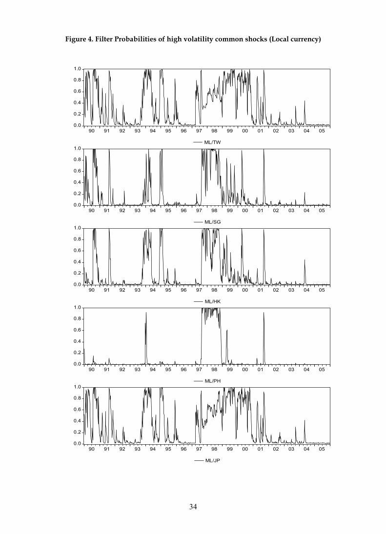
evidence of a change in the transmission of shocks between regimes. Figure 4

presents the filtered probabilities of being in the high-volatility regime and again

provide evidence in favor of adopting a regime-switching methodology.

Turning to the idiosyncratic shocks, we find that results, reported in Table 9,

are comparable to the USD returns. The impact coefficients are slightly higher in both

regimes; the average probability of being in the turbulent state decreases as for the

common shock but interestingly, the average duration of the shock remains about the

same. This suggests that in the previous analysis, the influence of the foreign

exchange risk largely affected the common shock only and is consistent with the

evidence in Figure 3.

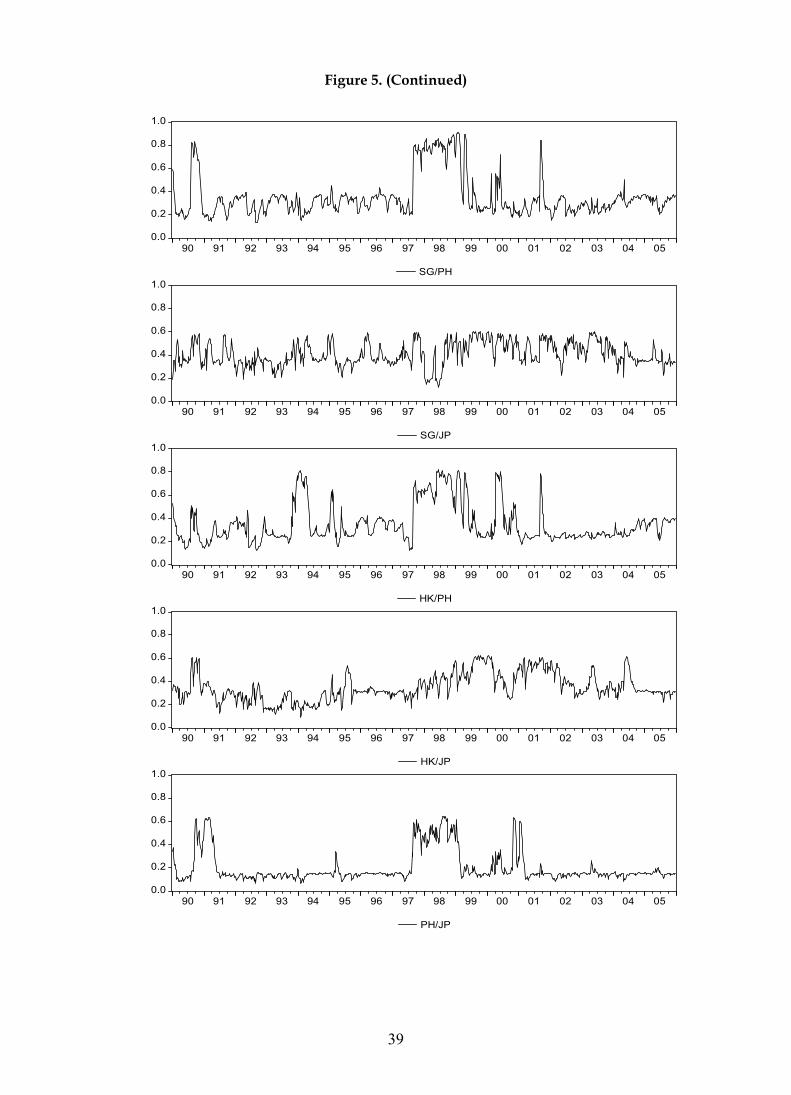
Figure 5 presents the conditional correlation for each market pair. The pattern

is similar to that of the earlier analysis. We observe a great deal of time variation but

only for pairs involving the Philippines is it different during the period of the Asian

crisis. For all other pairs, there is nothing to suggest that the behavior of the

correlation is different around the time of the crisis. In summary, our results appear

to be quite robust to the denomination of equity returns. We find little evidence of

contagion in either case.

5. Conclusions

We test for equity market contagion between six East Asian countries and

analyze the effectiveness of policy responses. We define ‘shift’ contagion as changes

in the transmission of structural shocks induced by a pair of markets being hit by a

common adverse shock. We use the methodology introduced by GKM, which is well

suited to our analysis. The main advantages of this methodology are that we can test

for contagion between countries without having to identify or including the source of

the shock, the crisis period is endogenously identified and we can disentangle the

contribution of volatility changes in both common and idiosyncratic shocks.

A regime-switching model is employed to exploit the heteroskedasticity

inherent in stock returns to identify whether or not we have contagion between each

15

pair of markets. We report a number of interesting findings. Firstly, expected stock

returns are statistically different between regimes. Calm markets are associated with

significantly positive returns while turbulent markets are characterized by negative

mean returns. Secondly, our model captures the features of return distributions quite

well. We find that common market shocks are, on average, in a high-volatility regime

about 27% of the time – though this varies substantially across market pairs. Thirdly,

we find little evidence of changes in the transmission of common shocks between

low- and high-volatility regimes. Hence, we reject the presence of shift contagion. In

its absence, we argue that policies designed to reinforce common market

fundamentals are likely to achieve their aim.

The idiosyncratic shocks also exert a major influence. This is best seen

through the evolution of the conditional correlations produced by the model. We

find that states characterized by high volatility in the common shock generate

relatively high pair wise correlation while, states where the country-specific shocks

are in the turbulent regime, generate lower correlations. Weighting each state by the

appropriate filtered probability enables us to construct the conditional correlation.

For all pairs, and consistent with Bordo and Murshid (2000), we observe significant

time variation in both calm and crisis periods. However, excluding pairs involving

the Philippines, there is no evidence that changes to the correlation were different

around the Asian crisis than those observed in earlier, more tranquil periods.

We check the robustness of our results by repeating the analysis for local

currency denominated returns. We find that our major results are unaffected. In

conclusion we find no support for the contagion in the East Asian markets during the

crisis of the late 1990’s.

Acknowledgments We would like to thank James Morley for making the

Gauss code available to us.

16

References

Ang, A., Bekaert, G., 2002. International asset allocation with regime shifts. Review of Financial studies, 15, 1137-1187.

Baur, D., Schulze, N., 2005. Co-exceedances in financial markets: a quantile regression analysis of contagion. Emerging Markets Review, 6, 21-43.

Bekaert, G., Harvey, C., 1995. Time-varying world market integration. Journal of Finance, 50(2), 403-444.

Bekaert, G., Harvey, C., Ng, A., 2005. Market integration and contagion. Journal of Business, 78(1), 39-69.

Bond, S., Dungey, M., Fry, R., 2006. A web of shocks: crises across Asian real estate markets. Journal of Real Estate Finance and Economics, 32(3), 253-274.

Bordo, M.D., Murshid, A.P., 2000. Are financial crises becoming increasingly more contagious? What is the historical evidence on contagion? NBER paper no. 7900.

Caporale, G., Cipollini, A., Spagnolo, N., 2003. Testing for contagion: a conditional correlation analysis. Journal of Empirical Finance, 12, 476-489.

Corsetti, G., Pericoli, M., Sbracia, M., 2001. Correlation analysis of financial contagion: what one should know before running a test. Banca d’Italia Temi di discussione, no. 408.

Dornbusch, R., Park, Y.C., Claessens, S., 2000. Contagion: understanding how it spreads. The World Bank Research Observer, 15(2), 177-197. Dungey, M., Fry, R., Martin, V., 2003. Equity transmission mechanisms from Asia to Australia: interdependence or contagion? Australian Journal of Management, 28(2), 157-182. Dungey, M., Fry, R., Martin, V., 2004. Currency market contagion in the Asia-Pacific region. Australian Economic Papers, 43(4), 379-395. Dungey, M., Fry, R., Martin, V., 2006. Correlation, contagion and Asian evidence. Asian Economic Journal, forthcoming. Flavin, T., Panopoulou, E, 2006. International Portfolio Diversification and Market Linkages in the presence of regime-switching volatility. IIIS Discussion paper No 167. Forbes, K.J., Rigobon, R.J., 2002. No contagion, only interdependence: measuring stock market comovements. Journal of Finance, 57 (5), 2223-61. Goetzmann, W., Li, L., Rouwenhorst, K.G., 2002. Long-term global market correlations. Working Paper no. 8612, National Bureau of Economic Research, Cambridge, MA.

17

Gravelle, T., Kichian, M., Morley, J., 2006. Detecting shift-contagion in currency and bond markets. Journal of International Economics, 68 (2), 409-423.

Guidolin, M., Timmermann, A., 2005. Economic implications of bull and bear regimes in UK stock and bond returns, Economic Journal, 115, 111-143. Hamilton, J.D., 1989. A new approach to the economic analysis of nonstationary time series and the business cycle, Econometrica, 57, 357-384.

Kaminsky, G.L., Schmukler, S.L., 1999. What triggers market jitters? A chronicle of the Asian crisis. Journal of International Money and Finance, 18, 537-560.

Karolyi, G.A., 2003. Does international financial contagion really exist? International Finance, 6(2), 179-199.

Karolyi, G. A., Stulz, R. M., 1996. Why Do Markets Move Together? An Investigation of U.S. – Japan Stock Return Co-movements, Journal of Finance, 51, 951–86. King, M.A., Wadhwani, S., 1990. Transmission of volatility between stock markets. Review of Financial Studies, 3, 5-33. Kleimeier, S., Lehnert, T., Verschoor, W., 2003. Contagion versus interdependence: a re-examination of Asian crisis stock market comovements. LIFE working paper 2003-05. Longin, F., Solnik, B., 1995. Is the correlation in international equity returns constant: 1960 – 1990? Journal of International Money and Finance, 14, 3-26. Pericoli, M., Sbracia, M., 2003. A primer on financial contagion. Journal of Economic Surveys, 17(4), 571-608. Rigobon, R., 2003a. Identification through heteroskedasticity. The Review of Economics and Statistics, 85(4), 777-792.

Rigobon, R., 2003b. On the measurement of the international propagation of shocks: is the transmission stable? Journal of International Economics, 61(2), 261-283.

18

Table 1: Summary Descriptive Statistics

Panel A: USD denominated (1/1/1990-31/12/2005)

Malaysia Taiwan Singapore Hong Kong Philippines Japan

Mean 0.053 -0.037 0.074 0.201 0.022 -0.023 Median 0.123 0.195 0.164 0.299 0.050 0.000

Maximum 46.149 21.969 21.143 16.487 25.352 15.772 Minimum -35.333 -24.728 -29.413 -25.798 -22.007 -12.078 Std. Dev. 4.789 4.894 3.291 3.850 4.241 3.244 Skewness 0.688 -0.241 -0.683 -0.633 0.138 0.163 Kurtosis 22.719 5.958 13.530 7.667 7.861 4.628

Jarque Bera 13594.0 (0.000)

312.5 (0.000)

3922.6 (0.000)

813.5 (0.000)

824.7 (0.000)

95.9 (0.000)

Panel B: Correlations

Market Malaysia Taiwan Singapore Hong Kong Philippines Japan Malaysia 1.000 0.254 0.558 0.481 0.399 0.259 Taiwan 1.000 0.375 0.327 0.289 0.205 Singapore 1.000 0.693 0.509 0.404 Hong Kong 1.000 0.472 0.356 Philippines 1.000 0.185 Japan 1.000

19

Table 2. Estimates of mean returns across regimes

Country pairs µ1 µ2 µ*1 µ*2 LR p-val ML/TW 0.302 0.102 -0.043 0.024 0.936 0.626 (0.093) (0.143) (0.042) (0.029) ML/SG 0.292 0.233 -1.176 -0.800 4.181 0.124 (0.090) (0.083) (0.638) (0.489) ML/HK 0.263 0.437 -1.090 -1.033 5.251* 0.072 (0.090) (0.104) (0.697) (0.633) ML/PH 0.248 0.126 -2.004 -0.769 2.101 0.350 (0.086) (0.106) (0.887) (0.482) ML/JP 0.285 0.065 0.055 -0.040 0.992 0.609 (0.107) (0.162) (0.138) (0.058) TW/SG 0.021 0.241 -0.088 -0.220 2.682 0.262 (0.051) (0.092) (0.408) (0.068) TW/HK 0.041 0.372 0.179 -0.581 1.629 0.443 (0.023) (0.096) (0.880) (0.989) TW/PH 0.095 0.128 -0.508 -0.484 0.852 0.653 (0.098) (0.102) (0.840) (1.193) TW/JP 0.315 0.090 -0.279 -0.115 3.311 0.191 (0.232) (0.105) (0.192) (0.154) SG/HK 0.279 0.455 -0.459 -0.461 4.618* 0.099 (0.094) (0.117) (0.425) (0.465) SG/PH 0.190 0.172 -0.640 -0.891 2.409 0.300 (0.092) (0.128) (0.607) (0.753) SG/JP 0.228 0.014 -0.034 -0.099 1.047 0.592 (0.086) (0.100) (0.253) (0.306) HK/PH 0.410 0.166 -0.463 -0.470 2.216 0.330 (0.067) (0.154) (0.134) (0.485) HK/JP 0.500 0.036 -0.045 -0.088 5.097* 0.078 (0.123) (0.038) (0.250) (0.096) PH/JP 0.164 0.018 -0.750 -0.366 1.771 0.413 (0.118) (0.042) (0.421) (0.151) Notes: Standard errors in parentheses below coefficients. Likelihood ratio statistic is for the null of equality of mean returns across the regimes. The test statistic has a )2(2χ distribution under the null hypothesis. *** denotes significance at 1% level, ** denotes significance at 5% level, and * denotes significance at 10% level.

20

Table 3. Estimates of impact coefficients of common shocks

Country pairs σc1 σc2 σ*c1 σ*c2 γ Unc. Prob. Duration ML/TW 1.957 0.920 4.749 1.482 1.506 34.39% 0.56 (0.084) (0.155) (0.382) (0.270) ML/SG 1.788 1.432 6.782 5.429 1.001 15.49% 0.23 (0.381) (0.356) (0.943) (0.520) ML/HK 1.578 1.444 6.700 6.152 1.004 14.80% 0.24 (0.319) (0.294) (0.667) (0.575) ML/PH 2.031 1.018 12.225 5.472 1.120 8.52% 0.53 (0.033) (0.054) (1.132) (0.828) ML/JP 1.179 1.164 3.234 1.164 2.744 41.08% 2.15 (0.451) (0.253) (0.256) (0.252) TW/SG 1.228 1.195 3.671 3.573 1.000 31.99% 0.22 (0.030) (0.339) (0.382) (0.251) TW/HK 1.677 2.006 4.326 5.205 1.005 16.83% 0.20 (0.209) (0.068) (0.517) (0.829) TW/PH 0.922 1.879 3.127 6.618 1.039 18.77% 0.45 (0.176) (0.507) (0.452) (0.728) TW/JP 0.094 0.100 2.495 2.169 1.213 58.84% 3.15 (0.142) (0.282) (0.405) (0.301) SG/HK 1.933 1.264 4.952 4.781 1.476 27.60% 0.21 (0.117) (0.173) (0.466) (0.532) SG/PH 1.360 1.374 5.787 5.934 1.015 13.85% 0.37 (0.211) (0.207) (0.531) (0.669) SG/JP 1.748 0.801 3.835 1.821 1.036 43.44% 0.32 (0.114) (0.237) (0.287) (0.182) HK/PH 1.528 1.347 5.740 5.061 1.000 18.14% 0.39 (0.234) (0.260) (0.537) (0.757) HK/JP 1.126 1.063 2.726 2.584 1.004 45.26% 2.94 (0.559) (0.154) (0.255) (0.212) PH/JP 1.575 0.521 7.023 2.315 1.003 14.70% 0.60 (0.127) (0.171) (0.672) (0.385)

Notes: Standard errors in parentheses below coefficients. “Duration” refers to the duration of the high volatility common shock expressed in years. “Unc. Prob.” refers to the unconditional probability of the high volatility regime expressed in percentage.

21

Table 4. Diagnostic tests on standardized residuals and model specification

Country pairs LM(1) LM(4) ARCH(1) ARCH(4) Normality RCM1 RCM2 RCM3 ML/TW 1.428 4.992 0.055 10.395 0.059 6.34 14.34 38.67 0.688 6.962 0.210 3.488 0.093 ML/SG 0.132 6.830 2.168 26.860* 0.088 14.49 18.85 20.18 0.549 2.679 36.374* 43.135* 0.067 ML/HK 0.030 6.710 0.959 10.752 0.071 12.23 37.95 17.55 0.285 3.348 0.007 1.755 0.104 ML/PH 0.409 7.072 0.864 8.424 0.065 32.91 30.52 5.69 0.089 13.168 0.253 4.387 0.027 ML/JP 0.055 4.409 2.755 14.995* 0.024 11.14 36.80 30.75 0.863 0.684 1.810 3.151 0.102 TW/SG 0.442 6.956 1.619 5.421 0.112 24.91 14.27 52.30 0.749 2.802 36.421* 44.112* 0.024 TW/HK 0.195 6.959 0.637 3.109 0.117 17.20 31.03 32.54 0.349 4.646 2.129 5.035 0.107 TW/PH 0.213 8.326 0.656 2.871 0.115 33.20 11.71 24.21 0.114 15.005* 2.412 9.931 0.033 TW/JP 0.561 7.070 0.189 2.533 0.091 27.57 67.86 40.64 0.826 1.817 0.035 1.368 0.042 SG/HK 0.001 1.743 18.088* 25.223* 0.061 23.75 35.92 37.12 0.154 5.451 3.555 9.337 0.097 SG/PH 0.007 1.437 25.145* 31.842* 0.035 64.31 38.04 15.46 0.249 10.815 0.811 8.142 0.052 SG/JP 0.232 2.986 5.448 10.366 0.044 5.18 37.95 52.52 0.844 0.716 0.670 1.771 0.077 HK/PH 1.336 3.721 2.507 3.400 0.083 40.69 29.65 22.98 0.196 13.061 0.332 7.067 0.035 HK/JP 1.384 4.990 7.064* 12.318 0.071 38.74 60.68 35.20 0.828 1.178 0.026 0.832 0.030 PH/JP 3.479 14.532* 0.196 6.916 0.029 68.80 61.63 16.36 0.526 1.134 0.020 1.364 0.049

Notes: LM(k) is the Breusch-Godfrey Lagrange Multiplier test for no serial correlation up to lag k,

ARCH(k) is the Lagrange Multiplier test for no ARCH effects of order k, Normality is the Cramer-von-

Mises test for the null of Normality, RCMi is the Regime Classification Measure, where i=1,2,3 for the

idiosyncratic shock of the first, second and the common shock, respectively. * denotes significance at 1%

level. LM(k) and ARCH(k) have a )(2 kχ distribution under the null hypothesis. The Cramer-von-Mises

test has a non-standard distribution and the cut-off value for RCM is 50.

22

Table 5. Likelihood ratio tests for shift contagion

Market Malaysia Taiwan Singapore Hong Kong Philippines Japan

Malaysia ---

1.422 (0.233)

6E-05 (0.994)

6E-05 (0.994)

0.205 (0.651)

2.773* (0.096)

Taiwan --- 0.0001 (0.991)

0.811 (0.368)

8E-05 (0.993)

0.0009 (0.976)

Singapore --- 0.370

(0.543) 2E-05 (0.996)

0.028 (0.868)

Hong Kong --- 0.0001 (0.991)

4E-05 (0.995)

Philippines --- 2E-05 (0.996)

Japan ---

Notes: Likelihood ratio statistic is for the null of no contagion against the alternative of contagion for the

indicated country pairs. The test statistic has a )1(2χ distribution under the null hypothesis. *** denotes significance at 1% level, ** denotes significance at 5% level, and * denotes significance at 10% level. p- values are reported in parentheses below coefficients.

23

Table 6. Estimates of impact coefficients of idiosyncratic shocks

Country pairs σ1 σ2 σ*1 σ*2 Unc. Prob./ Duration

(1)

Unc. Prob./ Duration (2)

ML/TW 0.034 3.919 11.745 8.999 8.01% 8.42% (0.066) (0.114) (1.320) (0.840) 0.97 0.42 ML/SG 1.313 1.325 9.390 2.736 10.83% 40.14% (0.593) (0.411) (1.076) (0.155) 0.14 5.56 ML/HK 1.499 1.853 7.915 3.666 15.62% 40.30% (0.330) (0.178) (0.626) (0.302) 0.71 1.22 ML/PH 0.349 2.725 4.308 6.292 25.78% 21.87% (0.440) (0.102) (0.424) (0.435) 0.52 0.33 ML/JP 1.401 1.522 11.066 3.367 11.76% 73.68% (0.405) (0.205) (0.978) (0.175) 0.24 1.48 TW/SG 3.107 1.331 7.597 4.169 16.38% 17.62% (0.052) (0.315) (0.578) (0.331) 0.30 2.30 TW/HK 3.242 0.949 8.432 3.464 12.02% 48.66% (0.135) (0.104) (0.682) (0.181) 0.35 2.28 TW/PH 3.402 2.208 7.677 7.001 18.96% 3.65% (0.170) (0.430) (0.261) (3.743) 0.20 0.04 TW/JP 3.177 1.799 8.035 3.719 17.06% 39.67% (0.195) (0.105) (0.677) (0.022) 0.21 0.21 SG/HK 0.018 1.760 2.486 3.249 11.13% 51.12% (0.024) (0.077) (0.561) (0.148) 0.68 1.83 SG/PH 1.082 2.436 2.802 5.042 43.96% 25.13% (0.224) (0.092) (0.204) (0.733) 0.32 0.43 SG/JP 0.048 1.666 7.264 3.274 3.61% 73.30% (0.249) (0.106) (1.331) (0.131) 0.47 1.37 HK/PH 1.265 2.546 3.018 5.372 68.17% 19.58% (0.237) (0.128) (0.111) (0.365) 2.02 0.48 HK/JP 1.849 1.727 4.887 3.862 31.52% 32.19% (0.151) (0.199) (0.379) (0.327) 0.41 0.19 PH/JP 2.021 1.904 4.167 3.787 30.71% 56.09% (0.068) (0.120) (0.616) (0.244) 0.13 0.36

Notes: Standard errors in parentheses below coefficients. “Duration” refers to the duration of the high volatility regime of the idiosyncratic shock expressed in years. “Unc. Prob.” refers to the unconditional probability of the high volatility regime expressed in percentage.

24

Table 7: Summary Descriptive Statistics

Panel A: Local currency (1/1/1990-31/12/2005)

Malaysia Taiwan Singapore Hong Kong Philippines Japan

Mean 0.092 -0.012 0.056 0.200 0.127 -0.050 Median 0.108 0.176 0.183 0.307 0.176 -0.163 Maximum 42.275 21.769 23.088 16.454 25.302 13.433 Minimum -35.333 -25.205 -31.698 -25.979 -28.127 -18.264 Std. Dev. 4.994 4.858 3.390 3.857 4.325 3.375 Skewness 0.362 -0.186 -0.885 -0.638 0.112 -0.155 Kurtosis 22.539 5.707 16.372 7.721 8.455 5.010

Jarque Bera 13301.0 (0.000)

259.8 (0.000)

6329.8 (0.000)

832.0 (0.000)

1037.1 (0.000)

144.0 (0.000)

Panel B: Correlations

Market Malaysia Taiwan Singapore Hong Kong Philippines Japan Malaysia 1.000 0.254 0.590 0.481 0.426 0.263 Taiwan 1.000 0.370 0.320 0.283 0.211 Singapore 1.000 0.681 0.516 0.433 Hong Kong 1.000 0.467 0.351 Philippines 1.000 0.211 Japan 1.000

25

Table 8. Estimates of impact coefficients of common shocks (Local currency)

Country pairs σc1 σc2 σ*c1 σ*c2 γ Unc. Prob. Duration ML/TW 1.955 0.759 4.965 1.599 1.205 30.37% 1.0 (0.083) (0.130) (0.338) (0.278) [0.661] ML/SG 1.668 1.436 7.007 6.035 1.000 14.72% 1.2 (0.230) (0.186) (0.921) (0.666) [0.999] ML/HK 1.501 1.528 5.887 5.990 1.001 17.57% 1.4 (0.398) (0.409) (0.659) (0.560) [0.969] ML/PH 1.947 1.034 13.381 6.578 1.080 8.19% 6.4 (0.118) (0.051) (1.267) (0.958) [0.970] ML/JP 1.956 0.658 5.027 1.316 1.286 29.96% 1.1 (0.147) (0.121) (0.320) (0.231) [0.432] TW/SG 0.994 1.271 2.898 3.718 1.003 40.09% 0.5 (0.011) (0.544) (0.374) (0.313) [0.987] TW/HK 1.664 1.838 4.513 4.982 1.001 17.75% 0.8 (0.361) (0.484) (0.750) (0.961) [0.984] TW/PH 0.989 1.689 3.616 6.153 1.004 17.96% 2.1 (0.034) (0.480) (0.532) (0.589) [0.967] TW/JP 1.370 1.896 3.148 6.318 1.450 6.89% 0.7 (0.122) (0.188) (0.174) (1.042) [0.386] SG/HK 1.525 1.550 4.599 4.678 1.001 29.55% 0.6 (0.243) (0.227) (0.428) (0.447) [0.999] SG/PH 1.383 1.491 6.712 6.946 1.042*** 10.48% 5.6 (0.700) (0.982) (0.763) (1.176) [0.000] SG/JP 1.742 0.897 3.919 1.991 1.014 41.64% 0.5 (0.145) (0.066) (0.228) (0.186) [0.968] HK/PH 1.544 1.527 6.047 5.921 1.010 14.25% 3.1 (0.689) (0.587) (0.447) (0.702) [0.968] HK/JP 1.742 1.140 3.713 2.425 1.002 33.09% 2.2 (0.924) (0.580) (0.799) (0.203) [0.992] PH/JP 1.523 0.789 6.995 2.610 1.389 14.35% 3.7 (1.280) (0.719) (0.382) (0.353) [0.890]

Notes: Standard errors in parentheses below coefficients. “Duration” refers to the duration of the high volatility common shock expressed in years. “Unc. Prob.” refers to the unconditional probability of the high volatility regime expressed in percentage. *** denotes significance at 1% level, ** denotes significance at 5% level, and * denotes significance at 10% level. p- values are reported in brackets below LR stat.

26

Table 9. Estimates of impact coefficients of idiosyncratic shocks (Local currency)

Country pairs σ1 σ2 σ*1 σ*2 Unc. Prob./ Duration

(1)

Unc. Prob./ Duration (2)

ML/TW 0.016 3.908 13.041 8.711 7.78% 8.85% (0.198) (0.116) (1.370) (0.941) 1.10 0.46 ML/SG 1.406 1.277 9.040 2.709 12.49% 38.47% (0.247) (0.198) (0.960) (0.235) 0.16 5.42 ML/HK 1.507 2.188 8.617 5.746 16.74% 6.11% (0.401) (0.301) (0.650) (1.788) 0.45 0.02 ML/PH 0.540 2.778 4.482 6.387 26.48% 20.46% (0.366) (0.107) (0.358) (0.493) 0.53 0.29 ML/JP 0.244 2.122 12.871 4.028 7.85% 50.52% (1.039) (0.352) (1.320) (0.379) 1.01 0.21 TW/SG 3.301 1.222 7.631 6.744 16.69% 5.07% (0.171) (0.552) (0.689) (1.055) 0.28 0.68 TW/HK 3.161 1.229 8.137 3.643 12.75% 46.83% (0.266) (0.673) (0.657) (0.447) 0.40 2.52 TW/PH 3.426 2.372 7.705 7.762 16.88% 5.78% (0.182) (0.326) (0.748) (1.792) 0.22 0.07 TW/JP 3.323 0.531 8.086 2.557 18.15% 79.84% (0.139) (0.216) (0.621) (0.158) 0.21 1.92 SG/HK 1.209 1.496 4.281 3.140 4.60% 52.16% (0.262) (0.210) (0.710) (0.220) 0.46 1.66 SG/PH 1.116 2.432 3.028 5.405 40.76% 23.86% (0.989) (0.549) (0.800) (0.502) 0.30 0.24 SG/JP 0.140 2.396 8.623 5.042 3.27% 17.28% (0.918) (0.134) (1.466) (0.664) 0.44 0.06 HK/PH 1.165 2.518 3.109 6.000 72.75% 16.13% (1.124) (0.402) (0.358) (0.549) 1.79 0.31 HK/JP 1.496 2.346 4.764 5.646 26.88% 11.40% (1.016) (0.213) (0.296) (0.817) 0.50 0.05 PH/JP 2.205 2.468 4.969 5.164 21.94% 18.67% (0.962) (0.155) (0.807) (0.490) 0.11 0.08

Notes: Standard errors in parentheses below coefficients. “Duration” refers to the duration of the high volatility regime of the idiosyncratic shock expressed in years. “Unc. Prob.” refers to the unconditional probability of the high volatility regime expressed in percentage.

27

Figure 1. Filter Probabilities of high volatility common shocks

0.0

0.2

0.4

0.6

0.8

1.0

90 91 92 93 94 95 96 97 98 99 00 01 02 03 04 05

ML/TW

0.0

0.2

0.4

0.6

0.8

1.0

90 91 92 93 94 95 96 97 98 99 00 01 02 03 04 05

ML/SG

0.0

0.2

0.4

0.6

0.8

1.0

90 91 92 93 94 95 96 97 98 99 00 01 02 03 04 05

ML/HK

0.0

0.2

0.4

0.6

0.8

1.0

90 91 92 93 94 95 96 97 98 99 00 01 02 03 04 05

ML/PH

0.0

0.2

0.4

0.6

0.8

1.0

90 91 92 93 94 95 96 97 98 99 00 01 02 03 04 05

ML/JP

28

Figure 1 (continued)

0.0

0.2

0.4

0.6

0.8

1.0

90 91 92 93 94 95 96 97 98 99 00 01 02 03 04 05

TW/SG

0.0

0.2

0.4

0.6

0.8

1.0

90 91 92 93 94 95 96 97 98 99 00 01 02 03 04 05

TW/HK

0.0

0.2

0.4

0.6

0.8

1.0

90 91 92 93 94 95 96 97 98 99 00 01 02 03 04 05

TW/PH

0.0

0.2

0.4

0.6

0.8

1.0

90 91 92 93 94 95 96 97 98 99 00 01 02 03 04 05

TW/JP

0.0

0.2

0.4

0.6

0.8

1.0

90 91 92 93 94 95 96 97 98 99 00 01 02 03 04 05

SG/HK

29

Figure 1 (continued)

0.0

0.2

0.4

0.6

0.8

1.0

90 91 92 93 94 95 96 97 98 99 00 01 02 03 04 05

SG/PH

0.0

0.2

0.4

0.6

0.8

1.0

90 91 92 93 94 95 96 97 98 99 00 01 02 03 04 05

SG/JP

0.0

0.2

0.4

0.6

0.8

1.0

90 91 92 93 94 95 96 97 98 99 00 01 02 03 04 05

HK/PH

0.0

0.2

0.4

0.6

0.8

1.0

90 91 92 93 94 95 96 97 98 99 00 01 02 03 04 05

HK/JP

0.0

0.2

0.4

0.6

0.8

1.0

90 91 92 93 94 95 96 97 98 99 00 01 02 03 04 05

PH/JP

30

Figure 2. Conditional Correlations

0.0

0.2

0.4

0.6

0.8

1.0

90 91 92 93 94 95 96 97 98 99 00 01 02 03 04 05

ML/TW

0.0

0.2

0.4

0.6

0.8

1.0

90 91 92 93 94 95 96 97 98 99 00 01 02 03 04 05

ML/SG

0.0

0.2

0.4

0.6

0.8

1.0

90 91 92 93 94 95 96 97 98 99 00 01 02 03 04 05

ML/HK

0.0

0.2

0.4

0.6

0.8

1.0

90 91 92 93 94 95 96 97 98 99 00 01 02 03 04 05

ML/PH

0.0

0.2

0.4

0.6

0.8

1.0

90 91 92 93 94 95 96 97 98 99 00 01 02 03 04 05

ML/JP

31

Figure 2 (continued)

0.0

0.2

0.4

0.6

0.8

1.0

90 91 92 93 94 95 96 97 98 99 00 01 02 03 04 05

TW/SG

0.0

0.2

0.4

0.6

0.8

1.0

90 91 92 93 94 95 96 97 98 99 00 01 02 03 04 05

TW/HK

0.0

0.2

0.4

0.6

0.8

1.0

90 91 92 93 94 95 96 97 98 99 00 01 02 03 04 05

TW/PH

0.0

0.2

0.4

0.6

0.8

1.0

90 91 92 93 94 95 96 97 98 99 00 01 02 03 04 05

TW/JP

0.0

0.2

0.4

0.6

0.8

1.0

90 91 92 93 94 95 96 97 98 99 00 01 02 03 04 05

SG/HK

32

Figure 2 (continued)

0.0

0.2

0.4

0.6

0.8

1.0

90 91 92 93 94 95 96 97 98 99 00 01 02 03 04 05

SG/PH

0.0

0.2

0.4

0.6

0.8

1.0

90 91 92 93 94 95 96 97 98 99 00 01 02 03 04 05

SG/JP

0.0

0.2

0.4

0.6

0.8

1.0

90 91 92 93 94 95 96 97 98 99 00 01 02 03 04 05

HK/PH

0.0

0.2

0.4

0.6

0.8

1.0

90 91 92 93 94 95 96 97 98 99 00 01 02 03 04 05

HK/JP

0.0

0.2

0.4

0.6

0.8

1.0

90 91 92 93 94 95 96 97 98 99 00 01 02 03 04 05

PH/JP

33

Figure 3. Exchange rates (vis-à-vis USD)

0

100

200

300

400

90 91 92 93 94 95 96 97 98 99 00 01 02 03 04 05

ML

0

4

8

12

16

90 91 92 93 94 95 96 97 98 99 00 01 02 03 04 05

TW

80

120

160

200

240

90 91 92 93 94 95 96 97 98 99 00 01 02 03 04 05

SG

0

100

200

300

400

90 91 92 93 94 95 96 97 98 99 00 01 02 03 04 05

HK

0

10

20

30

40

50

90 91 92 93 94 95 96 97 98 99 00 01 02 03 04 05

PH

1

2

3

4

5

6

90 91 92 93 94 95 96 97 98 99 00 01 02 03 04 05

JP

34

Figure 4. Filter Probabilities of high volatility common shocks (Local currency)

0.0

0.2

0.4

0.6

0.8

1.0

90 91 92 93 94 95 96 97 98 99 00 01 02 03 04 05

ML/TW

0.0

0.2

0.4

0.6

0.8

1.0

90 91 92 93 94 95 96 97 98 99 00 01 02 03 04 05

ML/SG

0.0

0.2

0.4

0.6

0.8

1.0

90 91 92 93 94 95 96 97 98 99 00 01 02 03 04 05

ML/HK

0.0

0.2

0.4

0.6

0.8

1.0

90 91 92 93 94 95 96 97 98 99 00 01 02 03 04 05

ML/PH

0.0

0.2

0.4

0.6

0.8

1.0

90 91 92 93 94 95 96 97 98 99 00 01 02 03 04 05

ML/JP

35

Figure 4. (continued)

0.0

0.2

0.4

0.6

0.8

1.0

90 91 92 93 94 95 96 97 98 99 00 01 02 03 04 05

TW/SG

0.0

0.2

0.4

0.6

0.8

1.0

90 91 92 93 94 95 96 97 98 99 00 01 02 03 04 05

TW/HK

0.0

0.2

0.4

0.6

0.8

1.0

90 91 92 93 94 95 96 97 98 99 00 01 02 03 04 05

TW/PH

0.0

0.2

0.4

0.6

0.8

1.0

90 91 92 93 94 95 96 97 98 99 00 01 02 03 04 05

TW/JP

0.0

0.2

0.4

0.6

0.8

1.0

90 91 92 93 94 95 96 97 98 99 00 01 02 03 04 05

SG/HK

36

Figure 4. (continued)

0.0

0.2

0.4

0.6

0.8

1.0

90 91 92 93 94 95 96 97 98 99 00 01 02 03 04 05

SG/PH

0.0

0.2

0.4

0.6

0.8

1.0

90 91 92 93 94 95 96 97 98 99 00 01 02 03 04 05

SG/JP

0.0

0.2

0.4

0.6

0.8

1.0

90 91 92 93 94 95 96 97 98 99 00 01 02 03 04 05

HK/PH

0.0

0.2

0.4

0.6

0.8

1.0

90 91 92 93 94 95 96 97 98 99 00 01 02 03 04 05

HK/JP

0.0

0.2

0.4

0.6

0.8

1.0

90 91 92 93 94 95 96 97 98 99 00 01 02 03 04 05

PH/JP

37

Figure 5. Conditional Correlations (Local currency)

0.0

0.2

0.4

0.6

0.8

1.0

90 91 92 93 94 95 96 97 98 99 00 01 02 03 04 05

ML/TW

0.0

0.2

0.4

0.6

0.8

1.0

90 91 92 93 94 95 96 97 98 99 00 01 02 03 04 05

ML/SG

0.0

0.2

0.4

0.6

0.8

1.0

90 91 92 93 94 95 96 97 98 99 00 01 02 03 04 05

ML/HK

0.0

0.2

0.4

0.6

0.8

1.0

90 91 92 93 94 95 96 97 98 99 00 01 02 03 04 05

ML/PH

0.0

0.2

0.4

0.6

0.8

1.0

90 91 92 93 94 95 96 97 98 99 00 01 02 03 04 05

ML/JP

38

Figure 5. (continued)

0.0

0.2

0.4

0.6

0.8

1.0

90 91 92 93 94 95 96 97 98 99 00 01 02 03 04 05

TW/SG

0.0

0.2

0.4

0.6

0.8

1.0

90 91 92 93 94 95 96 97 98 99 00 01 02 03 04 05

TW/HK

0.0

0.2

0.4

0.6

0.8

1.0

90 91 92 93 94 95 96 97 98 99 00 01 02 03 04 05

TW/PH

0.0

0.2

0.4

0.6

0.8

1.0

90 91 92 93 94 95 96 97 98 99 00 01 02 03 04 05

TW/JP

0.0

0.2

0.4

0.6

0.8

1.0

90 91 92 93 94 95 96 97 98 99 00 01 02 03 04 05

SG/HK

39

Figure 5. (Continued)

0.0

0.2

0.4

0.6

0.8

1.0

90 91 92 93 94 95 96 97 98 99 00 01 02 03 04 05

SG/PH

0.0

0.2

0.4

0.6

0.8

1.0

90 91 92 93 94 95 96 97 98 99 00 01 02 03 04 05

SG/JP

0.0

0.2

0.4

0.6

0.8

1.0

90 91 92 93 94 95 96 97 98 99 00 01 02 03 04 05

HK/PH

0.0

0.2

0.4

0.6

0.8

1.0

90 91 92 93 94 95 96 97 98 99 00 01 02 03 04 05

HK/JP

0.0

0.2

0.4

0.6

0.8

1.0

90 91 92 93 94 95 96 97 98 99 00 01 02 03 04 05

PH/JP

Institute for International Integration StudiesThe Sutherland Centre, Trinity College Dublin, Dublin 2, Ireland