CRITICAL EXPONENTS OF INDUCED DIRICHLET

FORMS ON SELF-SIMILAR SETS

Shi-Lei Kong and Ka-Sing Lau

Abstract

In [KLW], we studied certain random walks on the hyperbolic graphs X associ-

ated with the self-similar sets K, and showed that the discrete energy EX on X has

an induced energy form EK on K. The domain of EK is a Besov space Λα,β/22,2 where

α is the Hausdorff dimension of K and β is a parameter determined by the “return

ratio” of the random walk. In this paper, we consider the functional relationship

of EX and EK . In particular, we investigate the critical exponents of the β in the

domain Λα,β/22,2 in order for EK to be a Dirichlet form. We provide some criteria

to determine the critical exponents through the effective resistance of the random

walk on X, and make use of certain electrical network techniques to calculate the

exponents for some concrete examples.

Contents

1 Introduction· · · · · · · · · · · · · · · · · · · · · · · · · · · · · · · · · · · · · · 2

2 Preliminaries · · · · · · · · · · · · · · · · · · · · · · · · · · · · · · · · · · · · · 5

3 Harmonic functions and trace functions · · · · · · · · · · · · · · · · · · · · · 8

4 Effective resistances of EX · · · · · · · · · · · · · · · · · · · · · · · · · · · · · 12

5 The critical exponents of DX · · · · · · · · · · · · · · · · · · · · · · · · · · · · 17

6 Network reduction and examples · · · · · · · · · · · · · · · · · · · · · · · · · 26

7 Remarks and open problems · · · · · · · · · · · · · · · · · · · · · · · · · · · · 35

2010 Mathematics Subject Classification. Primary 28A80, 60J10; Secondary 60J50.Keywords: Besov space, Dirichlet form, hyperbolic graph, minimal energy, Martin boundary,

resistance, self-similar set, random walkThe research is supported in part by the HKRGC grant and the NNSF of China (no. 11371382).

1

1 Introduction

The theory of Dirichlet forms on a metric measure space was originated in the

seminal work of Beurling and Deny [BeD] as a generalization of the Laplacian on

Rd. Motivated by the development of fractals, in the past three decades, there has

been extensive study and development of this form from analytic and probabilistic

points of view. In [Jo], Jonsson studied the local regular Dirichlet form (E ,D) on

the Sierpinski gasket K. He showed that the domain DK is the Besov space Λα,β/22,∞

where α = log 3/ log 2 and β = log 5/ log 2. This consideration was extended by

Pietruska-Paluba to nested fractals and d-sets [P1, P2]. It has also been studied

amply in the general setting of metric measure space together with the heat kernel

estimates (e.g., [GH1, GH2, GHL1, GHL2, GHL4]). In another direction, Stos [St]

investigated the Dirichlet forms on a d-set K as a stable process subordinate to

the Brownian motion on K. He showed that E(β)K , 0 < β < 2, is non-local, and the

domain is another type of Besov space Λα,β/22,2 . For the associated stable processes,

the heat kernel was studied in detail by Chen and Kumagai [CK] on a d-set with

0 < β < 2. Recently, there is a great interest to study non-local regular Dirichlet

forms and the associated heat kernels of the jump processes on metric measure

spaces (e.g., [CKW1,CKW2,GHL3,GHH1,GHH2,HK]).

Let K be a compact subset in Rd and ν be an associated measure satisfying

ν(B(x, r)) � rα for any ball B(x, r) with center at x ∈ K and radius r > 0 (by

f � g, we mean f and g are positive functions, and C−1g ≤ f ≤ Cg for some

C > 0). We define the Besov space Λα,β/22,2 to be the Banach space contained in

L2(K, ν) with norm defined by

‖u‖Λα,β/22,2

= ‖u‖L2 +( ∫∫

K×K

|u(ξ)− u(η)|2

|ξ − η|α+βdν(ξ)dν(η)

)1/2. (1.1)

(Note that ν × ν vanishes on the diagonal.) It is easy to see that Λα,β/22,2 , β > 0 is

decreasing with increasing β, and it can be trivial for sufficiently large β. We define

the critical exponent β∗ of K by

β∗ = sup{β > 0 : Λα,β/22,2 contains nonconstant functions}.

The critical exponent plays an important role in the study of the Laplacian and

Brownian motion on fractals. It is where a local regular Dirichlet form (i.e., the

Laplacian) is expected to occur, and the domain is Λα,β∗/22,∞ . The β∗ is referred to

as the “walk dimension” of the underlying set K as it is the scaling exponent for

the space-time relation of the diffusive process: Ex(|Xt − x|2) ≈ t2/β∗. For the

special cases, we know that for Rd, β∗ = 2, and for the d-dimensional Sierpinski

gasket, β∗ = log(d+ 3)/ log 2 [Jo] (for planar SG, β∗ = log 5/ log 2 ≈ 2.322), and for

2

the Sierpinski carpet, it was estimated that β∗ ≈ 2.031 [B, BB]. In [GHL1], it was

proved that 2 ≤ β∗ ≤ α+ 1 under the assumption that a sub-Gaussian heat kernel

exists together with a chain condition. Despite the many developments, it is still

an open question whether a Laplacian will exist on some more general fractal sets.

In [KLW], we studied non-local Dirichlet forms with another approach. For a

self-similar set K with the open set condition (OSC), there is a hyperbolic graph

(X,E) (augmented tree) on the symbolic space of K, and the hyperbolic boundary is

Holder equivalent to K [Ka,LW1,LW2]. We introduced a class of transient reversible

random walks with return ratio λ ∈ (0, 1), called λ-natural random walk (λ-NRW)

on (X,E) with conductance c(x,y) depending on λ (see Section 2). We showed

that the Martin boundary, the hyperbolic boundary and K are homeomorphic, and

the hitting distribution ν is the normalized α-Hausdorff measure where α is the

dimension of K. Moreover, by using a theory of Silverstein [Si], it was proved that

the graph energy

E(λ)X [f ] =

1

2

∑x,y∈X

c(x,y)|f(x)− f(y)|2 (1.2)

defined by the random walk induces a positive definite bilinear form on K,

E(β)K (u, v) �

∫∫K×K

(u(ξ)− u(η))(v(ξ)− v(η))

|ξ − η|α+βdν(ξ)dν(η),

with β = log λ/ log r, where r is the minimum of the contraction ratios of the IFS

maps. Clearly the domain D(β)K = {u ∈ L2(K,µ) : E(β)

K [u] <∞} is the Besov space

Λα,β/22,2 .

In this paper we continue the investigation of the above induced bilinear func-

tional E(β)K . Our investigation has two main focuses, namely, to establish the func-

tional relationship of the discrete energy E(λ)X and the induced E(β)

K , then use it to

study the critical exponents ofD(β)K (i.e., Λ

α,β/22,2 ). LetD(λ)

X be the domain of E(λ)X , and

let DH(λ)X denote the class of harmonic functions in D(β)

K . For u ∈ D(β)K , we use Hu to

denote the Poisson integral of u on X, and for f ∈ D(λ)X , let Trf(ξ) = limxn→ξ f(xn).

By imposing a norm on D(λ)X , we prove (Theorem 3.5, Corollary 3.6)

Theorem 1.1. Suppose K is a self-similar set and assume that the OSC holds.

Then for a λ-NRW with λ ∈ (0, rα), we have D(β)K = Tr(DH(λ)

X ). Moreover, Tr is a

Banach space isomorphism on DH(λ)X , and Tr−1 = H.

The condition λ ∈ (0, rα) in Theorem 1.1 will be used throughout the paper. It

implies that β > α, and functions in D(β)K are Holder continuous (Proposition 2.5);

3

moreover, the convergence rate (λ/rα)n is essential when we consider functions in

DX that tend to the boundary K.

To consider the critical exponent of D(β)K , we introduce some finer classification

of the domains. We let

β∗1 := sup{β > 0 : D(β)K ∩ C(K) is dense in C(K)},

β∗2 := sup{β > 0 : dimD(β)K =∞}

β∗3 := sup{β > 0 : D(β)K contains nonconstant functions},

Clearly we have 2 ≤ β∗1 ≤ β∗2 ≤ β∗3 ≤ ∞, and β∗3 = β∗ for the β∗ defined above.

In the standard cases, these three exponents are equal, but there are also examples

that they are different [GuL]. It is one of the main purposes of this paper to discuss

these exponents and to provide some criteria to determine them. Our approach

relies on the effective resistance. We use R(λ)(ξ, η) to denote the effective resistance

for ξ, η ∈ K (see Section 4), and note that the infinite word i∞ of {Si}Ni=1 will

represent an element in K.

Theorem 1.2. With the assumptions as in Theorem 1.1, then D(λ)K consists of only

constant functions if and only if R(λ)(i∞, j∞) = 0 for all i, j = 1, · · · , N .

Consequently, if we let λ∗3 = sup{λ > 0 : R(λ)(i∞, j∞) = 0 ∀ i, j = 1, · · · , N},then β∗3 = log λ∗3/ log r (Thereom 5.4). Moreover if β∗3 > α and K is connected, we

have β∗2 = β∗3 (Theorem 5.6). For β∗1 , we give a result on the post critically-finite

(p.c.f.) sets [Ki1]. We let V0 denote the “boundary” of K.

Theorem 1.3. If in addition, K is a p.c.f. set and satisfies another mild geometric

condition (see Theorem 5.9). Then if

R(λ−ε)(ξ, η) > 0, ∀ ξ 6= η ∈ V0,

for some 0 < ε < λ, then D(β)K is dense in C(K) with supremum norm.

Consequently, if λ∗1 := inf{λ > 0 : R(λ)(ξ, η) > 0, ∀ ξ 6= η ∈ V0} ∈ (0, rα), then

β∗1 = log λ∗1/ log r.

A challenging task is to determine the effective resistance R(λ)(i∞, j∞) (or

R(λ−ε)(ξ, η) for ξ, η ∈ V0) to be = 0 or > 0 in the above theorems. For this we

make use of the basic tools in the electrical network theory (series and parallel

laws, ∆-Y transform, as well as cutting and shorting) to provide a device for such

estimation, which is applied to some special cases as examples.

4

For the organization of the paper, in Section 2, we summarize the needed results

from [KLW]. In Section 3, we prove some basic results on the extension of functions

on D(β)K be the Poisson integral, and the limit of function in D(λ)

X , and prove Theorem

1.1. We define and justify the limiting effective resistance in Section 4, and prove

Theorems 1.2 and 1.3 in Section 5. In Section 6, we make use of the electrical

techniques to give some implementations of the theorems by some examples. Some

remarks and open problems are provided in Section 7.

2 Preliminaries

We will give a brief summary of the background results in [KLW] for the convenience

of the reader, and all the unexplained notations can be found there. Let {Si}Ni=1,

N ≥ 2, be an iterated function system (IFS) of contractive similitudes on Rd with

contraction ratios {ri}Ni=1, and let K be the self-similar set. Let Σ∗ be the symbolic

space of K. Let r = min{ri : i = 1, · · · , N}. For n ≥ 1, define

Jn = {x = i1 · · · ik ∈ Σ∗ : rx ≤ rn < ri1···ik−1}, (2.1)

and J0 = {ϑ} by convention. Consider the modified symbolic space X =⋃∞n=0 Jn,

which has a tree structure with an edge set Ev. The tree structure can be strength-

ened to a hyperbolic graph by adding more horizontal edges on the tree according

to the neighboring cells on each level n [Ka, LW1, LW2]. According to [LW2], we

define

Eh = {(x,y) ∈ Jn × Jn : dist(Sx(K), Sy(K)) ≤ κrn, n ≥ 0},

where κ > 0 is arbitrary but fixed. Let E = Ev ∪ Eh, and call it an augmented

tree. It was shown that (X,E) is a hyperbolic graph in the sense of Gromov [Wo1].

In this case, the horizontal geodesic is uniformly bounded, and for any x,y ∈ X,

the canonical geodesic consists of three segments [x,u,v,y], where [x,u], [v,y] are

vertical paths in Ev, [u,v] is a horizontal geodesic in J` with the smallest `. Using

this geodesic, the Gromov product (x|y) = ` − h/2, where h is the length of [u,v].

We define a visual metric ρa(x,y) = e−a(x|y) on X for some a > 0. Let XH be the

completion, and define the hyperbolic boundary ∂HX = XH \ X. Then ∂HX is a

compact metric space.

A geodesic ray {xn}n is a sequence of words with xn = i1i2 · · · in ∈ Jn. If

ξ ∈ ∂HX has a canonical representation i1i2 · · · ∈ Σ∞, then {xn}n converges to

ξ, and ξ ∈ Sxn(K) for all n. It follows that for any other geodesic ray {yn}nconverging to ξ, we have xn ∼h yn. In the sequel, we will make use of the geodesic

rays frequently to relate functions on X and K. We call the sequence {κn}∞n=1 a

5

κ-sequence if each κn is a selection map from K to Jn, such that for each ξ ∈ K,

(κn(ξ))∞n=1 is a geodesic ray converging to ξ. It follows from the above that

Lemma 2.1. For any IFS {Si}Ni=1, let (X,E) be the hyperbolic graph as defined

above. Let E be a closed subset K. Then for any two κ-sequences {κn}∞n=1 and

{κ′n}∞n=1, we have

κ′n(E) ⊂ {x ∈ Jn : d(x, κn(E)) ≤ 1} for each n,

where d(·, ·) is the graph metric on (X,E).

Theorem 2.2. [LW2] For any IFS {Si}Ni=1, let (X,E) be the hyperbolic graph as

defined above. Then the hyperbolic boundary is Holder equivalent to the self-similar

set K, i.e., for the canonical map ι : ∂HX −→ K,

ρa(ξ, η)(= e−a(x|y)) � |ι(ξ)− ι(η)|−a/ log r.

Throughout, we will always assume that the IFS {Si}Ni=1 satisfies the open set

condition (OSC) [Fa]. In this case, the self-similar set K has Hausdorff dimension

α which is uniquely determined by∑N

i=1rαi = 1.

In [KLW], we introduced a class of reversible random walks on the augmented

tree (X,E): for λ ∈ (0, 1), we set the conductance c : E→ (0,∞) such that

c(x,x−) = rαxλ−|x|, and c(x,y) � rαxλ−|x|, x ∼h y ∈ X \ {ϑ}, (2.2)

where x− is the parent of x, rx := ri1 · · · rim for x = i1 · · · im. We define the natural

random walk with return ratio λ ∈ (0, 1) (λ-NRW) to be the Markov chain {Zn}∞n=0

on X with transition probability P (x,y) = c(x,y)/m(x) if x ∼ y, and 0 otherwise,

where m(x) =∑

y:x∼y c(x,y) is the total conductance at x ∈ X. Note that the chain

moves forward and backward with a ratio λ ∈ (0, 1); hence {Zn}∞n=0 is transient.

LetM denote the Martin boundary, and let Z∞ be the pointwise limit of {Zn}∞n=0,

starting from ϑ.

Theorem 2.3. [KLW] Let {Si}Ni=1 be an IFS satisfying the open set condition, and

let {Zn}∞n=0 be a λ-NRW. Then

(i) the distribution ν of Z∞ on M is the α-Hausdorff measure;

(ii) the Martin kernel K(x, ξ) � λ|x|−(x|ξ)r−α(x|ξ);

(iii) the Martin boundary M, the hyperbolic boundary ∂HX, and the self-similar

set are all homeomorphic.

6

It follows from part (iii) that we can carry Doob’s discrete potential theory onto

the self-similar set K. We denote the space of harmonic functions (w.r.t. P ) on X

by H(X) = {f ∈ `(X) : Pf = f}, where `(X) is the collection of real functions on

X, and Pf(x) =∑

y∈X P (x,y)f(y). The Poisson integral for u ∈ L1(K, ν) is

Hu(·) =

∫KK(·, ξ)u(ξ)dν(ξ) ∈ H(X). (2.3)

The graph energy of f ∈ `(X) is given by

EX [f ] =1

2

∑x,y∈X:x∼y

c(x,y)(f(x)− f(y))2, (2.4)

and the domain of EX is DX = {f ∈ `(X) : EX [f ] < ∞}. Using Silverstein’s

theorem [Si], together with Theorem 2.3 (iii), we obtain an induced quadratic form

on K.

Theorem 2.4. [KLW] Under the assumptions in Theorem 2.3, the graph energy

in (2.4) induces an energy form EK [u] given by

EK [u] := EX [Hu] =m(ϑ)

2

∫∫K×K

|u(ξ)− u(η)|2Θ(ξ, η)dν(ξ)dν(η), u ∈ L2(K, ν),

(2.5)

where Θ(ξ, η) � (λrα)−(ξ|η) � |ξ − η|−(α+β) (Naim kernel) with β = log λlog r .

By definition, the domain of EK is DK = {u ∈ L2(K, ν) : Hu ∈ DX}. It

follows from the above that DK is the Besov space Λα,β/22,2 . If we define ‖u‖2EK =

EK [u]+‖u‖2L2(K,ν), then (DK , ‖ ·‖EK ) is a Banach space, and is equivalent to Λα,β/22,2 .

For γ > 0, we let

Cγ(K) = {u ∈ C(K) : ‖u‖Cγ := ‖u‖∞ + esssupξ,η∈K|u(ξ)− u(η)||ξ − η|γ

<∞} (2.6)

denote the Holder space. We will use the following result frequently. It was proved

in [GHL1] (the assumption of heat kernel stated there is not needed in the proof)

that

Proposition 2.5. If β > α, then for all u ∈ L2(K, ν),

‖u‖Cγ ≤ C‖u‖Λα,β/22,2

(2.7)

with γ = (β − α)/2. Consequently, Λα,β/22,2 ↪→ Cγ is an imbedding.

It follows that for α < β < β∗1 , DK ∩ C(K) = DK is trivially dense in DKunder the norm ‖ · ‖EK , and in C(K) under the supremum norm. This implies that

(EK ,DK) is a non-local regular Dirichlet form.

7

3 Harmonic functions and trace functions

In this section, we will set up a natural relation between harmonic functions on X

with finite graph energy and continuous functions on K with finite induced energy

(Theorem 3.5). First we use Theorem 2.3(ii) to provide a “uniform tail estimate” of

the Martin kernel. As in [KLW, Section 5], we introduce a projection ι : X → K by

selecting ι(x) ∈ Sx(O∩K) arbitrarily, where O is an open set in the OSC satisfying

O ∩K 6= ∅.

Proposition 3.1. Let {Si}Ni=1 be an IFS satisfying the OSC, and let {Zn}∞n=0 be

a λ-NRW on the augmented tree (X,E). Then for any ε, δ > 0, there exists a

positive integer n0 such that for any x ∈ X and |x| ≥ n0, K(x, ξ) ≤ ε holds for any

ξ ∈ K \B(ι(x), δ).

Proof. It follows from Theorem 2.3(ii) that

K(x, ξ) ≤ C1λ|x|(λrα)−(x|ξ), x ∈ X, ξ ∈ K.

Note that (x|ξ) ≤ (ι(x)|ξ) by [KLW, Lemma 3.9(ii)]. Hence for ξ ∈ K \B(ι(x), δ),

r−(x|ξ) ≤ r−(ι(x)|ξ) ≤ C2|ι(x)− ξ|−1 ≤ C2δ−1,

(the second inequality follows from Theorem 2.2 (see also [LW2, Theorem 1.2]).

Hence for ε > 0, we can pick positive integer n0 such that the last inequality in the

following holds:

K(x, ξ) ≤ C1λn0r−(α+log λ/ log r)(x|ξ) ≤ C1λ

n0(C2δ−1)α+log λ/ log r ≤ ε.

Let νx, x ∈ X, denote the hitting distribution of Z∞ on K, starting from x. As

K(x, ·) = dνx/dν, the above result shows that the mass of the distribution νx will

concentrate around ι(x) (equivalently, Sx(K)) as |x| → ∞. We have a Fatou-type

theorem as a corollary.

Corollary 3.2. Suppose {Si}Ni=1 satisfies OSC, and let {Zn}∞n=0 be a λ-NRW on

the augmented tree (X,E). Then for u ∈ C(K) and ε > 0, there exists a positive

integer n0 such that

|Hu(x)− u(ξ)| ≤ ε (3.1)

whenever |x| ≥ n0 and ξ ∈ Sx(K). In particular, limn→∞Hu(xn) = u(ξ) uniformly

for ξ ∈ K, where {xn}n is a geodesic ray converging to ξ.

8

Proof. Since u is continuous on the compact set K, u is bounded and uniformly

continuous. We let supξ∈K |u(ξ)| = M0 < ∞ and choose δ > 0 such that |u(ξ) −u(η)| < ε/3 whenever |ξ−η| < δ on K. Furthermore, by Proposition 3.1, we choose

n0 such that both diam(Sx(K)) ≤ δ and K(x, ξ) ≤ ε6M0

hold for any x ∈ X with

|x| ≥ n0 and ξ ∈ K \B(ι(x), δ). Then for |x| ≥ n0, by using the usual technique of

splitting the following integral on K into K ∩B(ι(x), δ) and K \B(ι(x), δ), we can

show that

|Hu(x)− u(ι(x))| ≤∫K|K(x, η)(u(η)− u(ι(x)))|dν(η) ≤ ε

Hence for ξ ∈ Sx(K),

|Hu(x)− u(ξ)| ≤ |Hu(x)− u(ι(x))|+ |u(ι(x))− u(ξ)| ≤ 2ε

3+ε

3= ε,

and (3.1) holds. For the last statement, let {xn}n be a geodesic ray converging to

ξ, then xn = i1 · · · in, and this i1i2 · · · ∈ Σ∞ is a representation of some ξ′ with

ξ′ ∈ Sxn(K), and ξ′ = ξ in ∂HX. Hence by (3.1), we have limn→∞Hu(xn) =

u(ξ′) = u(ξ), and the convergence is uniform on ξ.

In the rest of this section, we assume that the λ-NRW has a return ratio λ ∈(0, rα). Then β = log λ/ log r > α, and Proposition 2.5 applies.

Lemma 3.3. Suppose {Si}Ni=1 satisfies OSC, and let {Zn}∞n=0 be a λ-NRW on the

augmented tree (X,E) with λ ∈ (0, rα). Then for f ∈ DX ,

(i) there exists C > 0 (depend on f) such that for any geodesic ray {xn}n,

|f(xn+1)− f(xn)| ≤ C(λ/rα)n/2,

and hence limn→∞

f(xn) exists;

(ii) for two equivalent geodesic rays (xn)n and (yn)n, limn→∞

f(xn) = limn→∞

f(yn).

Proof. (i) Let τ = λ/rα < 1. For a geodesic ray (xn)n, since

|f(xn+1)− f(xn)| ≤

√EX [f ]

c(xn+1,xn)≤ C(λ/rα)n/2 = Cτn/2,

hence the sequence (f(xn))n converges in an exponential rate.

(ii) For two equivalent geodesic rays (xn)n and (yn)n that converge to the same

ξ, if they are distinct, then xn ∼h yn for all n (or by Lemma 2.1). Then

|f(xn)− f(yn)| ≤

√EX [f ]

c(xn,yn)≤ C ′τn/2, (3.2)

which tends to 0 as n→∞. Hence the two limits are equal.

9

With the assumption as in Lemma 3.3, we can define a linear map Tr : DX →`(K) (called a trace map) by

(Trf)(ξ) = limn→∞

f(xn), ξ ∈ K, (3.3)

where (xn)n is a geodesic ray that converges to ξ. We call Trf the trace function of

f . By Lemma 3.3(ii), the limit in (3.3) is “uniform” in the sense as follows.

Proposition 3.4. Suppose {Si}Ni=1 satisfies OSC, and let {Zn}∞n=0 be a λ-NRW

with ratio λ ∈ (0, rα) on the augmented tree (X,E). Then the limit in (3.3) is

uniform, in the sense that for f ∈ DX and ε > 0, there exists a positive integer n0

such that

|f(x)− Trf(ξ)| ≤ ε (3.4)

whenever |x| ≥ n0 and ξ ∈ Sx(K). Moreover, Trf is continuous on K.

Proof. The first part follows from Lemma 3.3. To prove the second part, for ε > 0,

by (3.4), we can pick a positive integer n0 such that |f(x)−Trf(ξ)| < ε/3 whenever

|x| ≥ n0 and ξ ∈ Sx(K). Since the length of the horizontal geodesics in (X,E)

is uniformly bounded [LW1, LW2], say by M . Also let C be a constant such that

c(x,y) ≥ C−1(rα/λ)|x| for all x ∼h y. By assumption τ := λ/rα < 1. We choose

n1 ≥ n0 such that M√CEX [f ]τn1 < ε/3.

As |ξ − η| � r(ξ|η) (Theorem 2.2), we can pick δ > 0 such that (ξ|η) ≥ n1

whenever |ξ − η| < δ. Now for ξ, η ∈ K with |ξ − η| < δ, consider a canonical

geodesic [ξ,u,v, η] with horizontal geodesic π(u,v) = [u = u0,u1, . . . ,uk = v] (see

Section 2). Then |u| ≥ (ξ|η) ≥ n1, and hence

|Trf(ξ)− Trf(η)| ≤ |Trf(ξ)− f(u)|+ |f(u)− f(v)|+ |f(v)− Trf(η)|

<ε

3+

k−1∑i=0

|f(ui)− f(ui+1)|+ ε

3

<2ε

3+M

√CEX [f ]τn1 < ε. (by (3.2))

This concludes that Trf ∈ C(K).

Theorem 3.5. Suppose {Si}Ni=1 satisfies the OSC, and let {Zn}∞n=0 be a λ-NRW

with ratio λ ∈ (0, rα) on the augmented tree (X,E). Then Tr(DHX) = DK where

DHX is the class of harmonic functions in DX . More precisely, TrHu = u for

u ∈ DK , and HTrf = f for f ∈ DHX .

10

Proof. For u ∈ DK , by definition we have Hu ∈ DHX . Note that DK∩C(K) = DK ,

as DK = Λα,β/22,2 can be imbedded into the Holder space C(β−α)/2(K) if β > α

(Proposition 2.5). By Corollary 3.2, we have TrHu = u.

For f ∈ DHX , let u = Trf ∈ C(K) (by Proposition 3.4). For any ε > 0, by

Corollary 3.2 and Proposition 3.4, there exists a positive integer n0 such that for

|x| ≥ n0 and ξ ∈ Sx(K),

|f(x)− u(ξ)| < ε

2and |Hu(x)− u(ξ)| < ε

2. (3.5)

Suppose that f 6= Hu. Assume without loss of generality that f(x0) > Hu(x0)

for some x0 ∈ Jm. Let an = maxx∈Jn(f(x)−Hu(x)), n ≥ 1. Note that f −Hu is

harmonic. By the Maximum Principle of harmonic functions, we regard Jn+1 as the

boundary of Xn+1 =⋃n+1k=0 Jk. Then an+1 ≥ maxx∈Xn(f(x) − Hu(x)) = an, thus

the sequence {an} is non-decreasing. Hence infn≥m an = am > 0. This contradicts

that limn→∞ an = 0 by (3.5). We conclude that f = Hu = HTrf .

In the above theorem, we can actually give a norm on DX so that H : DK →DHX is a Banach space isomorphism. Indeed, by Proposition 3.4 and the continuity

of functions in DK , we know that functions in DX are bounded. Fix w ∈ (0, rα),

let ‖f‖2`2(X,w) =∑

x∈X |f(x)|2w|x|, and define ‖ · ‖EX on DX by

‖f‖2EX = EX [f ] + ‖f‖2`2(X,w), (3.6)

Then it is direct to check that ‖f‖2EX defines a complete norm on DX .

Corollary 3.6. With the same assumption as in Theorem 3.5 and let w ∈ (0, rα).

Then for all u ∈ L2(K, ν),

‖Hu‖`2(X,w) ≤ C‖u‖L2(K,ν). (3.7)

Consequently, H : (DK , ‖ · ‖EK )→ (DHX , ‖ · ‖EX ) is an isomorphism.

Proof. Let F (x,y) denote the probability that the random walk ever visits y from

x. For n ≥ 1 and |y| > n, by [KLW, Theorem 4.6],

F (ϑ,y) =∑x∈Jn

Fn(ϑ,x)F (x,y) =∑x∈Jn

rαxF (x,y) ≥ rα(n+1)∑x∈Jn

F (x,y).

Hence∑

x∈Jn K(x, ξ) =∑

x∈JnF (x,y)F (ϑ,y) ≤ r

−α(n+1). It follows that for u ∈ L2(K, ν),

‖Hu‖2`2(X,w) =∑

x∈X

(Ex(u(Z∞))

)2w|x| ≤

∑x∈X

(Ex(u(Z∞)2)

)w|x|

=∑∞

n=0wn

∑x∈Jn

∫KK(x, ξ)|u(ξ)|2dν(ξ) ≤ C‖u‖2L2(K,ν).

11

where C = r−α∑∞

n=0(w/rα)n. As w/rα < 1, this yields (3.7). In view of Theorem

3.5, the norm isomorphism of the map H : DK → DHX follows from this and

EK(u, v) = EX(Hu,Hv), and the open mapping theorem.

4 Effective resistances of EXIn this section, we will set up the limiting effective resistance for the λ-NRW on

the augmented tree (X,E) in order to prepare for the investigation of the critical

exponents of DK in the next section.

We will start with a general situation. Let V be a finite graph with a reversible

Markov chain with conductance c(x, y), x, y ∈ V . Let `(V ) denote the class of real

valued functions on V , and let EV (f) be the graph energy of f . For any V1 ⊂ V ,

it is well-known that each f ∈ `(V1) has an harmonic extension to V , which has

a minimal energy among all g ∈ `(V ) with g|V1 = f . In the following, we give an

expression of the minimal energy in terms of the conductance c(x, y) of the chain

on V .

Proposition 4.1. Let V be a finite set, and V = V1∪V2 with #V1 ≥ 2. Assume that

there is a reversible Markov chain on V with conductance c(·, ·). Then for f ∈ V1,

min{EV [g] : g ∈ `(V ), g|V1 = f

}=

1

2

∑x,y∈V1,x 6=y

c∗(x, y)(f(x)− f(y))2, (4.1)

where c∗(x, y) = c(x, y) +∑

z,w∈V2 c(x, z)GV2(z, w)P (w, y), x, y ∈ V1, x 6= y (here

GV2(·, ·) is the Green function of the random walk restricted to V2), and it defines a

conductance function on V1.

Proof. Let F V1(x, y) = Px(ZtV1 = y) where tV1 is the first hitting time of V1. Then

F V1(z, y) =∑

w∈V2GV2(z, w)P (w, y), ∀x ∈ V2, y ∈ V1.

We can check directly from the definition that c∗(x, y) = c∗(y, x), x, y ∈ V1, using

the reversibility of the chain (i.e., m(x)P (x, z) = m(z)P (z, x) and m(z)GV2(z, w) =

m(w)GV2(w, z)). Hence c∗(x, y) defines a conductance on V1.

To prove (4.1), we let h(·) =∑

y∈V1 FV1(·, y)f(y) ∈ `(V ). Then it is easy to

check that h is the unique function such that Ph = h on V2 and h = f on V1. Hence

EV [h] = min{EV [g] : g ∈ `(V ), g|V1 = f}. Observe that

EV [h] =1

2

∑x,y∈V

c(x, y)(h(x)− h(y))2 =∑x,y∈V

c(x, y)(h(x)− h(y))h(x)

12

Hence

EV [h] =∑x∈V1

h(x)∑y∈V

c(x, y)(h(x)− h(y)) (by Ph = h on V2)

=∑x∈V1

f(x)( ∑y∈V1

c(x, y)(f(x)− f(y)) +∑y∈V2

c(x, y)∑z∈V1

F V1(y, z)(f(x)− f(z)))

=∑x,y∈V1

f(x)(f(x)− f(y))(c(x, y) +

∑z∈V2

c(x, z)F V1(z, y))

(switch y and z)

=∑x,y∈V1

c∗(x, y)f(x)(f(x)− f(y))

=1

2

∑x,y∈V1

c∗(x, y)(f(x)− f(y))2. (use c∗(x, y) = c∗(y, x))

This yields (4.1).

For a finite connected graph (X,E) with conductances, the effective resistance

between two disjoint nonempty subsets A, B ⊆ X is given by

RX(E,F ) = (min{EX [f ] : f ∈ `(X) with f = 1 on E, and f = 0 on F})−1. (4.2)

Also we set RX(E,F ) = 0 if E∩F 6= ∅ by convention. Clearly RX(·, ·) is symmetric,

and the energy minimizer in (4.2) is unique, bounded in between 0 and 1, and is

harmonic on X \ (E ∪ F ).

For the λ-NRW on (X,E), for convenience and the simplicity in the estimations,

we will assume slightly more that the conductance on the horizontal edges satisfies

c(x,y) = rα|x|λ−|x| for x ∼h y ∈ X \ {ϑ}. (4.3)

(we use � in (2.2)), and there is no change of the results. Let {κn}∞n=1 be a κ-

sequence defined in Section 2. For any two closed subsets Φ, Ψ ⊆ K, we define the

level-n resistance between them (depend on κn) by

R(λ)n (Φ,Ψ) := RXn(κn(Φ), κn(Ψ)), (4.4)

where Xn := ∪nk=0Jk and has same conductance restricted from X.

Theorem 4.2. Suppose {Si}Ni=1 satisfies the OSC, and let {Zn}∞n=0 be a λ-NRW

on the augmented tree (X,E) with λ ∈ (0, rα). Then for any two closed subsets Φ,

Ψ ⊆ K, the limit limn→∞R(λ)n (Φ,Ψ) exists, and is independent of the choice of the

κ-sequence.

13

We will prove a technical lemma first. For E,F ⊂ Jn such that in the graph

distance, dist(E,F ) > 2, we define

∂E = {x ∈ Jn : dist(x, E) = 1}, ∂F = {x ∈ Jn : dist(x, F ) = 1}. (4.5)

Let En := En(E,F ) = min{EXn [f ] : f ∈ `(Xn), f = 1 on E, f = 0 on F}, and let f

be the energy minimizing function.

Lemma 4.3. Consider the λ-NRW on (X,E) with λ ∈ (0, rα). Let {En}n≥1, {Fn}n≥1

be two sequences such that En, Fn ⊂ Jn, and lim infn→∞ dist(En, Fn) > 2. If

supn≥1 En(En, Fn) <∞, then for any ε > 0, there exists n0, such that for n ≥ n0,

∑x∈∂En

∑y∈Xn\En

c(x,y)(1− f(y))2 < ε,∑

x∈∂Fn

∑y∈Xn\Fn

c(x,y)f(y)2 < ε,

where f is the energy minimizer of En := En(En, Fn).

Proof. We observe that

En =1

2

∑x,y∈Xn

c(x,y)(f(x)− f(y))2

=∑

x,y∈Xn

c(x,y)f(x)(f(x)− f(y))

=∑x∈En

∑y∈Xn

c(x,y)(1− f(y)) ≥ (rα/λ)n∑

y∈∂En

(1− f(y)) (4.6)

(the third equality holds because f is harmonic on Xn \ (En ∪ Fn)). Thus f(x) ≥1 − (λ/rα)nEn for x ∈ ∂En. Using a similar argument, and that f is harmonic on

Xn \ (En ∪ Fn ∪ ∂En), for large n, we have

En ≥1

2

∑x,y∈Xn

c(x,y)(f(x)− f(y))2 −∑

x∈∂En

∑y∈En

c(x,y)(f(x)− f(y))2

=∑

x∈∂En

f(x)∑

y∈Xn\En

c(x,y)(f(x)− f(y)) +∑y∈En

c(y,y−)(1− f(y−))

≥(1− (λ/rα)nEn

) ∑x∈∂En

∑y∈Xn\En

c(x,y)(f(x)− f(y)) (4.7)

(The inequality is valid because for x ∈ ∂En, by harmonicity,∑

y∈Xn\En c(x,y)(f(x)−f(y)) = −

∑y∈En c(x,y)(f(x)− f(y)) = −

∑y∈En c(x,y)(f(x)− 1) ≥ 0).

14

Now we use (4.6) and (4.7) to make the final estimate:∑x∈∂En

∑y∈Xn\En

c(x,y)(1− f(y))2

≤ λn

rα(n+1)

( ∑x∈∂En

∑y∈Xn\En

c(x,y)(1− f(y)))2

=λn

rα(n+1)

( ∑x∈∂En

∑y∈Xn\En

c(x,y)((1− f(x)) + (f(x)− f(y))

))2

≤ λn

rα(n+1)

(kEn +

En1− (λ/rα)nEn

)2

=: ε(n)(by (4.6), (4.7)

)(4.8)

where k = supx∈X #{y : x ∼h y} (as the graph (X,E) has bounded degree, and

c(x,y) > 0 only when x ∼h y or y = x−). Hence we can choose n0 such that

ε(n) < ε for n > n0. Analogously, using 1− f instead of f , we obtain the estimate

for F as well.

Proof of Theorem 4.2. We fix a λ ∈ (0, rα) and omit the superscript (λ) in this

proof. First we fix a κ-sequence {κn}∞n=0, and prove that limn→∞Rn(Φ,Ψ) exists.

For brevity, we write Φn := κn(Φ) and Ψn := κn(Ψ). If Φ ∩ Ψ 6= ∅, then by the

property of geodesic rays in (X,E), for any n, either Φn∩Ψn 6= ∅ or min{d(x,y) : x ∈Φn, y ∈ Ψn} = 1 (by Lemma 2.1). In both situations, we have limn→∞Rn(Φ,Ψ) = 0

(for the second case, by (4.2), Rn(Φ,Ψ) ≤ (rαnλ−n)−1 = (λ/rα)n).

Hence we assume that Φ ∩Ψ = ∅. Then there exists ` > 0 such that for n ≥ `,

dist(Φn,Ψn) > 3. By (4.2) and (4.4), for n ≥ `,

Rn(Φ,Ψ) = (min{EXn [f ] : f = 1 on Φn, and f = 0 on Ψn})−1. (4.9)

Let En denote the minimal energy, and let fn ∈ `(Xn) be the energy minimizer in

(4.9). Let {nk}k≥1 with nk ≥ ` be the subsequence such that limk→∞Rnk(Φ,Ψ) =

lim supn→∞Rn(Φ,Ψ) > 0. (otherwise limn→∞Rn(Φ,Ψ) = 0). Then supk Enk < ∞.

For n < nk and ξ ∈ K, by Lemma 3.3(i), we have

|fnk(κn(ξ))− fnk(κnk(ξ))| ≤nk−n∑m=1

|fnk(κn+m−1(ξ))− fnk(κn+m(ξ))|

≤ C( λrα

)n/2:= ε(n). (4.10)

As λ ∈ (0, rα), limn→∞ ε(n) = 0. Let V1 = Φn ∪ Ψn. Then for sufficiently large n

15

and nk > n, we have ε(n) < 12 , and

Enk ≥ EXn [fnk ] ≥ min{EXn [f ] : f ∈ `(Xn), f = fnk on V1}

=1

2

∑x,y∈V1

c∗(x,y)(fnk(x)− fnk(y))2 (by Proposition 4.1)

≥∑x∈Φn

∑y∈Ψn

c∗(x,y)(fnk(x)− fnk(y))2

≥∑x∈Φn

∑y∈Ψn

c∗(x,y)((1− 2ε(n))2 (by (4.10))

= min{EXn [f ] : f ∈ `(Xn), f |Φn = 1− 2ε(n), f |Ψn = 0}(by Proposition 4.1)

= (1− 2ε(n))2En.

Therefore, Rn(Φ,Ψ) ≥ (1 − 2ε(n))2Rnk(Φ,Ψ) for any large n and nk > n. Taking

limit, we have

lim infn→∞

Rn(Φ,Ψ) ≥ limk→∞

Rnk(Φ,Ψ) = lim supn→∞

Rn(Φ,Ψ).

Hence limn→∞Rn(Φ,Ψ) exists.

Next we show that the above limit is independent of the choice of the κ-sequence.

For this, we define

∂Φn = {x ∈ Jn : d(x,Φn) = 1}, ∂Ψn = {x ∈ Jn : d(x,Ψn) = 1}

as in (4.5). For any other κ-sequences {κ′n}n, it follows from Lemma 2.1 that

κ′n(Φ) ⊂ Φn ∪ ∂Φn and κ′n(Ψ) ⊂ Ψn ∪ ∂Φn. Hence it suffices to show that

limn→∞

RXn(Φn ∪ ∂Φn,Ψn ∪ ∂Φn) = limn→∞

Rn(Φ,Ψ). (4.11)

Without loss of generality, we assume limn→∞Rn(Φ,Ψ) > 0. Then supn En <

∞. Let hn ∈ `(Xn) with hn = 1 on ∂Φn, hn = 0 on ∂Ψn, and hn = fn on

Xn \ (∂Φn ∪ ∂Ψn).

0 ≤ RXn(Φn ∪ ∂Φn,Ψn ∪ ∂Φn)−1 −Rn(Φ,Ψ)−1 ≤ EXn [hn]− EXn [fn].

Then by Lemma 4.3, for given ε, and for large n, EXn [hn] − EXn [fn] ≤ 2ε. This

implies (4.11) and proves the theorem.

Theorem 4.2 implies the following definition is well defined.

Definition 4.4. With the same assumption as in Theorem 4.2, we define the (lim-

iting) effective resistance between two closed subsets Φ and Ψ in K by

R(λ)(Φ,Ψ) := limn→∞

R(λ)n (Φ,Ψ). (4.12)

(We omit the superscript (λ) if there is no confusion.)

16

5 The critical exponents of DX

We use the trace function to establish a basic result on the existence of nonconstant

functions in DK .

Theorem 5.1. With the same assumption as in Theorem 4.2, suppose Φ,Ψ are two

closed subsets of K satisfying R(Φ,Ψ) > 0. Then there exists u := uΦ,Ψ ∈ DK such

that u = 1 on Φ, and u = 0 on Ψ. Moreover, uΦ,Ψ is the unique energy minimizer

in DK in the following sense

R(Φ,Ψ)−1 = EK [uΦ,Ψ] = inf{EK [u′] : u′ ∈ DK with u′ = 1 on Φ, u′ = 0 on Ψ}.(5.1)

Proof. First we show that the set on the right in (5.1) is non-empty. Clearly Φ∩Ψ =

∅ (otherwise R(Φ,Ψ) = 0). Fix a κ-sequence {κn}n. As in the proof of Theorem

4.2, there exists a positive integer ` such that κn(Φ) ∩ κn(Ψ) = ∅ for all n ≥ `, let

fn ∈ `(Xn) be the energy minimizer for κn(Φ) and κn(Ψ) as in (4.9). We extend

fn to X by setting fn(x) = 0 for x ∈ X \Xn, then fn is harmonic on Xn−1. Note

that 0 ≤ fn ≤ 1 for all n ≥ `. Hence for each x ∈ X, there exists a convergent

subsequence of {fn(x)}n≥`. By the diagonal argument, we can find a subsequence

{fnk}k≥1 with n1 ≥ ` such that fnk converges to a function f ∈ `(X) pointwise. We

claim that

(a) f ∈ DHX and 0 ≤ f ≤ 1 on X;

(b) For any ξ ∈ Φ, limn→∞ f(κn(ξ)) = 1;

(c) For any η ∈ Ψ, limn→∞ f(κn(η)) = 0.

In fact, as fnk is harmonic on Xnk−1, the pointwise limit f is harmonic on X. For

k ≥ 1, let gk be the function on the edge set E defined by: for (x,y) ∈ E,

gk(x,y) =

{c(x,y)(fnk(x)− fnk(y))2, if x,y ∈ Xnk ,

0, otherwise.

Then Enk := EXnk [fnk ] = 12

∑(x,y)∈E gk(x,y), and limk→∞ gk(x,y) = c(x,y)(f(x)−

f(y))2. By Fatou’s Lemma, we have

EX [f ] =1

2

∑(x,y)∈E

c(x,y)(f(x)− f(y))2 =1

2

∑(x,y)∈E

(limk→∞

gk(x,y)

)≤ 1

2lim infk→∞

∑(x,y)∈E

gk(x,y) = limk→∞

Enk = R(Φ,Ψ)−1 <∞. (5.2)

Hence (a) follows.

17

To prove (b), observe that R(Φ,Ψ) > 0 implies that supk≥1 Enk <∞. Hence for

any k ≥ 1, n < nk and ξ ∈ Φ, by Lemma 3.3(i)

|fnk(κn(ξ))− 1| ≤nk−1∑m=n

|fnk(κm(ξ))− fnk(κm+1(ξ))| ≤ C1(λ/rα)n/2.

Letting k →∞, we have |f(κn(ξ))− 1| ≤ C2(λ/rα)n/2, hence (b) follows by letting

n→∞. With a similar argument, we can also conclude (c).

By the claim and Theorem 3.5, let u = Trf ∈ DK . Then 0 ≤ u ≤ 1 on K,

u(ξ) = limn→∞ f(κn(ξ)) = 1 for all ξ ∈ Φ, and u(η) = limn→∞ f(κn(η)) = 0 for all

η ∈ Ψ.

Now we complete the proof of the theorem. By (5.2), EK [uΦ,Ψ] = EX [fΦ,Ψ] ≤R(Φ,Ψ)−1. For the reverse inequality, it suffices to show that R(Φ,Ψ)−1 ≤ EK [u]

for all u ∈ DK with u = 1 on Φ and u = 0 on Ψ. Fix a κ-sequence {κn}n. For any

ε ∈ (0, 12), by Proposition 3.2, there exists a positive integer n0 = n0(ε) such that

|Hu(κn(ξ)) − u(ξ)| ≤ ε whenever n ≥ n0 and ξ ∈ K. Taking V1 = κn(Φ) ∪ κn(Ψ)

and g = Hu|V1 as in Proposition 4.1, then we have, for n ≥ n0,

min{EXn [f ] : f ∈ `(Xn), f = Hu on V1} =1

2

∑x,y∈V1

c∗(x,y)(Hu(x)−Hu(y))2.

(5.3)

Hence

EXn [Hu] ≥ min{EXn [f ] : f ∈ `(Xn), f = Hu on V1}

≥∑

x∈κn(Φ)

∑y∈κn(Ψ)

c∗(x,y)(Hu(x)−Hu(y))2 (by (5.3))

≥∑

x∈κn(Φ)

∑y∈κn(Ψ)

c∗(x,y)((1− ε)− ε

)2= (1− 2ε)2Rn(Φ,Ψ)−1.

As ε can be arbitrarily small, we have R(Φ,Ψ)−1 ≤ limn→∞ EXn [Hu] = EK [u].

Hence (5.1) follows.

The uniqueness of uΦ,Ψ as an energy minimizer follows from the fact that EK is

strictly convex in DK .

The function f ∈ DHX thus constructed is called a harmonic function induced

by Φ and Ψ. The function u = Trf ∈ DK is referred as the energy minimizer of Φ

and Ψ. We denote them by fΦ,Ψ and uΦ,Ψ respectively.

18

Corollary 5.2. With the same assumption as in Theorem 4.2, the following con-

ditions are equivalent: for two distinct points ξ, η ∈ K,

(i) there exists u ∈ DK with range [0, 1] such that u(ξ) = 1 and u(η) = 0;

(ii) there exists u ∈ DK such that u(ξ) 6= u(η);

(iii) R(ξ, η) > 0.

In this case, R(ξ, η) = sup{ |u(ξ)− u(η)|2

EK(u, u): u ∈ DK , EK(u, u) > 0

}.

Proof. Note that (i) ⇒ (ii) is trivial, and (iii) ⇒ (i) follows from Theorem 5.1.

We need only prove (ii) ⇒ (iii). We observe that the given u ∈ DK is continuous

(Proposition 2.5). Fix any κ-sequence, by Corollary 3.2, there exists n0 > 0 such

that for n ≥ n0, |Hu(κn(ξ)) − u(ξ)| ≤ 13 |u(ξ)− u(η)|, and the same for η. Hence

|Hu(κn(ξ))−Hu(κn(η))| ≥ 13 |u(ξ)− u(η)|. Then by (4.2), for n > n0

|u(ξ)− u(η)|2

9Rn(ξ, η)≤ |Hu(κn(ξ))−Hu(κn(η))|2

Rn(ξ, η)

≤ c(κn(ξ), κn(η)) |Hu(κn(ξ))−Hu(κn(η))|2 ≤ EXn [Hu].

Taking the limit on n, we have |u(ξ)−u(η)|29R(ξ,η) ≤ EK [u] <∞. Hence R(ξ, η) > 0.

Corollary 5.3. With the same assumption as in Theorem 4.2, if R(λ)(ξ, η) = 0,

then β∗1 ≤ log λ/ log r where β∗1 := sup{β > 0 : D(β)K ∩ C(K) is dense in C(K)}.

Proof. If R(λ)(ξ, η) = 0, then every u ∈ DK must satisfy u(ξ) = u(η), so DK is not

dense in C(K), which implies β∗1 ≤ log λ/ log r.

Remark. For the implication of (ii)⇒ (iii) in Corollary 5.2, we can omit λ ∈ (0, rα)

(i.e., β > α), but consider u ∈ DK ∩ C(K), and replace R(ξ, η) by R(ξ, η) :=

lim infn→∞Rn(ξ, η), then the implication still holds. Consequently, Corollary 5.3 is

still valid.

In the following, we will apply Corollary 5.2 to give some criteria to determine

the critical exponents for β∗2 := sup{β > 0 : dimD(β)K = ∞} and β∗3 := sup{β > 0 :

D(β)K contains nonconstant functions}.

Let in = ii · · · i ∈ Jn denote the unique word in level n consisting of symbol i ∈ Σ,

and let i∞ = ii · · · ∈ Σ∞ (identified with the point ξ = limn Sin(K) in K). Then for

two distinct symbols i, j ∈ Σ, we use R(i∞, j∞) to denote the effective resistance

for the corresponding two points in K, and R(i∞, j∞) = limn→∞Rn(i∞, j∞).

19

Theorem 5.4. With the same assumption as in Theorem 4.2, then DK consists of

only constant functions if and only if

R(λ)(i∞, j∞) = 0, ∀ i, j ∈ Σ. (5.4)

Consequently, β∗3 = log λ∗3/ log r if

λ∗3 := sup{λ > 0 : R(λ)(i∞, j∞) = 0, ∀ i, j ∈ Σ} ∈ (0, rα), (5.5)

and β∗3 =∞ if the above set of λ is empty.

Proof. If for some i, j ∈ Σ, R(i∞, j∞) > 0, then there exists u ∈ DK with u(i∞) 6=u(j∞) by Proposition 5.1 (or by Corollary 5.2 (iii) ⇒ (ii)). Thus it suffices to show

that (5.4) implies DK = {constant functions}.First we claim that for u ∈ C(K), if u(xi∞) = u(xj∞) for any x ∈ Σ∗ and

i, j ∈ Σ, then u is a constant function. Indeed, let c = u(1∞), then choosing x = ϑ

we have u(i∞) = c for any i ∈ Σ. Choosing x = i we have u(ij∞) = u(i∞) = c

hence u(xj∞) = c for any x ∈ Σ1 and j ∈ Σ. Following the similar arguments,

inductively we have u(xj∞) = c for any x ∈ Σ∗ and j ∈ Σ. By continuity, u ≡ c is

constant.

For nonconstant u ∈ C(K), by the claim we can pick x ∈ Σ∗ and i, j ∈ Σ such

that u(xi∞) 6= u(xj∞). We telescope u on the cell Sx(K) to get u = u ◦ Sx. Then

u(i∞) 6= u(j∞). By Proposition 5.3 (or by Corollary 5.2 (ii)⇒ (iii)) and assumption

(5.4), we must have u /∈ DK . Note that

EK [u] ≥ c1

∫Sx(K)

∫Sx(K)

|u(ξ)− u(η)|2

|ξ − η|α+βdν(ξ)dν(η)

≥ c2

∫K

∫K

|u(ξ)− u(η)|2

|ξ − η|α+βdν(ξ)dν(η) ≥ c3EK [u], (5.6)

hence u /∈ DK . Finally as DK ∩C(K) = DK by Theorem 2.2, DK contains constant

functions only.

Next we will show that β∗2 = β∗3 under the connectedness of the self-similar set.

The following lemma is a key step to include more non-trivial functions in DK .

Lemma 5.5. With the same assumption as in Theorem 4.2, suppose ξ ∈ K and Ψ

is a closed subset in K satisfying R(ξ,Ψ) > 0. Let u = uξ,Ψ ∈ DK be the limiting

harmonic function. Then for η ∈ K such that 0 < u(η) < 1, we have R(η,Ψ) > 0

and R(ξ,Ψ ∪ {η}) > 0.

20

Proof. Let f = fξ,Ψ = Hu and ε = min{u(η), 1 − u(η)} > 0. Fix a κ-sequence

{κn}n. By Proposition 3.2, there exists a positive integer m0 such that

|f(κn(η))− u(η)| < ε/4, ∀n ≥ m0. (5.7)

Following the same argument as in the proof of Proposition 5.1, let fn ∈ `(Xn) be

the energy minimizer in (4.9) with Φ = {ξ}. By passing to subsequence, we assume,

without loss of generality, that fn ∈ `(X) converges to f pointwise.

Note that for n ≥ 1 and k < n, by Lemma 3.3(i),

|fn(κk(η))− fn(κn(η))| ≤n−1∑m=k

|fn(κm(η))− fn(κm+1(η))| ≤ C1(λ/rα)k/2.

Thus we can pick a positive integer m1 ≥ m0 such that

|fn(κm1(η))− fn(κn(η))| < ε/4, ∀n ≥ m1. (5.8)

Since fn(κm1(η)) → f(κm1(η)) as n → ∞, there exists a positive integer n0 such

that n0 ≥ m1 and

|fn(κm1(η))− f(κm1(η))| < ε/4, ∀n ≥ n0. (5.9)

Combining (5.7)–(5.9), we have fn(κn(η)) ∈ (ε/4, 1 − ε/4) for all n ≥ n0. Using

(4.2) and (4.4), for n ≥ n0, we have

Rn(η,Ψ) ≥ fn(κn(η))2

EXn [fn]>ε2

16Rn(ξ,Ψ). (5.10)

Hence R(η,Ψ) > 0 by passing limit.

To prove R(ξ,Ψ ∪ {η}) > 0, let gn ∈ `(Xn) be the energy minimizer in (4.9)

with Φ = {η}. By passing to subsequence if necessary, we let γ1,n = fn(κn(η)) and

γ2,n = gn(κn(ξ)). Then γ1,nγ2,n ∈ [0, 1− ε/4) as γ1,n ∈ (ε/4, 1− ε/4) (by last part)

and γ2,n ∈ [0, 1]. For n ≥ 1, we can check that the function

hn :=1

1− γ1,nγ2,nfn −

γ1,n

1− γ1,nγ2,ngn ∈ `(Xn)

satisfies hn(κn(ξ)) = 1, and hn = 0 on κn(Ψ ∪ {η}). Moreover, hn is harmonic on

Xn \ κn(Ψ ∪ {ξ, η}), thus EXn [hn] = (Rn(ξ,Ψ ∪ {η}))−1 by (4.4). Hence

R(ξ,Ψ ∪ {η}) = limn→∞

(EXn [hn])−1 ≥ limn→∞

(2EXn [fn]

(1− γ1,nγ2,n)2+

2γ21,nEXn [gn]

(1− γ1,nγ2,n)2

)−1

≥ limn→∞

(2

(ε/4)2Rn(ξ,Ψ)+

2(1− ε/4)2

(ε/4)2Rn(η,Ψ)

)−1

=

(2

(ε/4)2R(ξ,Ψ)+

2(1− ε/4)2

(ε/4)2R(η,Ψ)

)−1

> 0.

21

Theorem 5.6. With the assumptions in Theorem 4.2, assume further K is con-

nected, and there exists β > α such that DK(= D(β)K ) is non-trivial. Then β∗2 = β∗3 .

Proof. It suffices to verify that for λ ∈ (0, rα), dimDK > 1 (⇔ DK contains noncon-

stant functions) implies that dimDK =∞. We have R(ξ, η) > 0 for some ξ, η ∈ Kby Corollary 5.2 (ii) ⇒ (iii). The energy minimizer u1 = uξ,η ∈ DK is continuous

with u1(ξ) = 1 and u1(η) = 0, hence there exists η1 ∈ K such that u1(η1) = 1/2. By

Lemma 5.5, we have R(ξ, {η, η1}) > 0 and this induces another energy minimizer

u2 = uξ,{η,η1} ∈ DK with u2(ξ) = 1 and u2(η) = u2(η1) = 0. By the continuity,

we can pick η2 ∈ K such that u2(η2) = 1/2. Setting η0 = η and repeating the

above argument, we get a sequence of energy minimizers {un}∞n=1 together with a

sequence of points {ηk}∞k=0 in K such that un(ξ) = 1, un(ηn) = 1/2, and un(ηk) = 0

for any 0 ≤ k < n. Thus [ui(ηj)]i,j≥1 is an infinite upper triangular matrix with

constant diagonal entries 1/2. Hence {un}∞n=1 is a sequence of linearly independent

functions in DK , so that dimDK =∞.

Remark. The connectivity of K is necessary in Theorem 5.6. For example, if we

let {Si}4i=1 be an IFS on R as follows:

S1(x) =x

4, S2(x) =

x

4+

1

12, S3(x) =

x

4+

2

3, S4(x) =

x

4+

3

4.

Then K = [0, 1/3] ∪ [2/3, 1], and it is easy to check that the IFS satisfies the OSC

(let O = (0, 1/3) ∪ (2/3, 1) as the open set). As K consists of two intervals as

connected components, we have β∗2 = 2, β∗3 =∞.

In the rest of this section, we focus on the post critically finite (=p.c.f.) self-

similar sets [Ki1], and provide a criterion to determine β∗1 . We will need a general

lemma as follow.

Lemma 5.7. With the same assumption as in Theorem 4.2, for a finite set E ⊂ Kwith #E ≥ 2, if R(ξ, η) > 0 for all distinct ξ 6= η in E, then R(ξ, E \ {ξ}) > 0 for

all ξ ∈ E.

Proof. We prove the lemma by induction on #E. It is trivial if #E = 2. Suppose

the lemma holds for #E = m (m ≥ 2). Now let #E = m+1. We choose arbitrarily

three distinct points ξ1, ξ2, ξ3 ∈ E. Then it suffices to show that R(ξ1, E \{ξ1}) > 0.

By induction hypothesis, we have three positive effective resistances R1 := R(ξ1, E \{ξ1, ξ2}), R2 := R(ξ2, E \ {ξ2, ξ3}) and R3 := R(ξ3, E \ {ξ3, ξ1}).

For sufficiently large n, let f1,n, f2,n, f3,n ∈ `(Xn) be the energy minimizer

in (4.9) with (Φ,Ψ) = ({ξ1}, E \ {ξ1, ξ2}), ({ξ2}, E \ {ξ2, ξ3}), ({ξ3}, E \ {ξ3, ξ1})respectively. Fix a κ-sequence {κn}n. Let γ1,n = f1,n(κn(ξ2)), γ2,n = f2,n(κn(ξ3)),

22

and γ3,n = f3,n(κ(ξ1)). Then γi,n ∈ [0, 1] for i = 1, 2, 3. For sufficiently large n, we

can check that the function

hn :=1

1 + γ1,nγ2,nγ3,n

(f1,n − (γ1,nf2,n + γ1,nγ2,nf3,n)

)(5.11)

satisfies hn(κn(ξ1)) = 1, and hn = 0 on κn(E \ ξ1). Moreover, hn is harmonic on

Xn \ κn(E), thus EXn [hn] = (Rn(ξ1, E \ {ξ1}))−1 by (4.4). Hence

R(ξ1, E \ {ξ1}) = limn→∞

(EXn [hn])−1

≥ limn→∞

(3(EXn [f1,n] + γ2

1,nEXn [f2,n] + γ21,nγ

22,nEXn [f3,n])

(1 + γ1,nγ2,nγ3,n)2

)−1

=

(3(R−1

1 + γ21,nR

−12 + γ2

1,nγ22,nR

−13 )

(1 + γ1,nγ2,nγ3,n)2

)−1

> 0.

This completes the proof of the induction.

Following Kigami [Ki1], for an IFS {Sj}Nj=1 with a self-similar set K, we let

CK =⋃i,j∈Σ,i 6=j(Si(K) ∩ Sj(K)), and define a critical set by C = π−1(CK), a post

critical set by P =⋃n≥1 σ

n(C). We call K post critically finite (p.c.f.) if P is a

finite set.

It is known that for the similitudes Sj = rj(Rjx + bj), j = 1, · · · , N , if the

{Rj}Nj=1 are commensurable, then the p.c.f. property implies the OSC [DL], and the

statement is not true without the commensurable assumption [TKV]. We introduce

two geometric conditions on the p.c.f. sets:

(C) for any family of distinct subcells Si1(K), · · · , Sik(K) that intersects at a point

p, there exists 0 < δ < 1 and closed cones Cj , 1 ≤ j ≤ k with vertex at p such that

Sij (K) ∩B(p, δ) ⊂ Cj , and Cj ∩ C` = {p} ∀ 1 ≤ j, ` ≤ k, j 6= `;

(H) there exists constant γ > 0 such that for any x,y ∈ X with |x| = |y|, if

Sx(K) ∩ Sy(K) = ∅, then

dist(Sx(K), Sy(K)) > γ · r|x|.

Condition (C) says the intersecting cells are separated by closed cones (except at

the vertices), and the geometric meaning is clear. Condition (H) says that if two

cells are disjoint, then they are “strongly” separate; it has been used in [Jo], [LW1]

and [GuL]. Note that the familiar self-similar sets satisfies this condition, and it is

proved in [GuL] the if the IFS is of the form Sj(x) = r(x+ bj) and is p.c.f., then K

satisfies condition (H).

23

Lemma 5.8. Let K be a p.c.f. self-similar set that satisfies either (C) or (H).

Suppose for α < β < β′, u satisfies u ◦ Si ∈ Λα,β′/22,2 for each i ∈ Σ, then u ∈ Λ

α,β/22,2 .

Proof. First suppose that K satisfies (C). By the separation of the cones, and the

cosine law of a triangle, we can show that there exists c > 0 such that if Si(K)

intersects Sj(K) at p, and for ξ ∈ Si(K) ∩B(p, δ), η ∈ Sj(K) ∩B(p, δ),

|ξ − η| ≥ c(|ξ − p|+ |η − p|) ≥ 2c|ξ − p|1/2 · |η − p|1/2. (5.12)

Since u ◦ Si ∈ Λα,β′/22,2 , it follows from Theorem 2.2 that u ◦ Si ∈ C(β′−α)/2(K).

As u(ξ) =∑N

i=1 u(ξ)χSi(K)(ξ), we show that u is also Holder continuous of order

(β′ − α)/2 at any p ∈ Si(K) ∩ Sj(K). Indeed we observe that for ξ ∈ Si(K) ∩B(p, δ), η ∈ Sj(K) ∩B(p, δ),

|u(ξ)− u(η)| ≤ |u(ξ)− u(p)|+ |u(η)− u(p)|

≤ C(|ξ − p|(β′−α)/2 + |η − p|(β′−α)/2)

≤ 2C(|ξ − p|+ |η − p|)(β′−α)/2

≤ C1|ξ − η|(β′−α)/2 (by (5.12)).

This together with (5.12) imply∫Si(K)∩B(p,δ)

∫Sj(K)∩B(p,δ)

|u(ξ)− u(η)|2

|ξ − η|α+βdν(ξ)dν(η)

≤ C2

∫Si(K)∩B(p,δ)

dν(ξ)

|ξ − p|α+β−β′ ·∫Sj(K)∩B(p,δ)

dν(η)

|η − p|α+β−β′ <∞. (5.13)

Now as u(ξ) =∑N

i=1 u(ξ)χSi(K)(ξ), we have

EK [u] =N∑

i,j=1

∫Si(K)

∫Sj(K)

|u(ξ)− u(η)|2

|ξ − η|α+βdν(ξ)dν(η)

=(∑i=j

+∑i 6=j

) ∫Si(K)

∫Sj(K)

|u(ξ)− u(η)|2

|ξ − η|α+βdν(ξ)dν(η)

:=SI + SII .

By a change of variable,

SI =n∑i=1

rα−βi

∫K

∫K

|u ◦ Si(ξ)− u ◦ Si(η)|2

|ξ − η|α+βdν(ξ)dν(η) <∞.

By (5.13), it is easy to check that SII < ∞. This shows that EK [u] < ∞, so that

u ∈ DK = Λα,β/22,2 .

24

Next we suppose that K satisfies (H). Assume without loss of generality that

diam(K) = 1. For p ∈ Si(K)∩Sj(K), i 6= j ∈ Σ, let δ = 12 min{|p− q| : q ∈ Si(K)∩

Sj(K), q 6= p}. Following the same argument in the last paragraph, it suffices to

show that (5.12) holds for ξ ∈ Si(K)∩B(p, δ) and η ∈ Sj(K)∩B(p, δ). Indeed, sup-

pose that |η−p| ≤ |ξ−p| ∈ (rk, rk−1] for some positive integer k. Let x,y ∈ Jk with

ξ ∈ Sx(K) ⊂ Si(K) and η ∈ Sy(K) ⊂ Sj(K). As diam(Sx(K)),diam(Sy(K)) ≤ rk,Sx(K) ∩ Sy(K) = ∅. Hence by condition (H),

|ξ − η| ≥ γ · rk ≥ γr|ξ − p| ≥ γr

2(|ξ − p|+ |η − p|).

This completes the proof.

We let V0 = π(P) be the “boundary” of a p.c.f. set K, and let Vn = ∪x∈ΣnSx(V0),

n ≥ 1.

Theorem 5.9. With the same assumption as in Theorem 4.2, assume further K is

a p.c.f. set with boundary V0 and satisfies (C) or (H), then DK is dense in C(K)

with supremum norm if

R(λ−ε)(ξ, η) > 0, ∀ ξ 6= η ∈ V0, (5.14)

for some ε ∈ (0, λ). Consequently, β∗1 = log λ∗1/ log r if

λ∗1 := inf{λ > 0 : R(λ)(ξ, η) > 0, ∀ ξ 6= η ∈ V0} ∈ (0, rα), (5.15)

and β∗1 ≤ α otherwise.

Proof. Let V0 = {ξ1, ξ2, · · · , ξm}. If R(ξi, ξj) = 0 for some i 6= j, then DK is

not dense in C(K) by Proposition 5.3. Now suppose that (5.14) holds and let

β0 = log(λ − ε)/ log r. Then R(λ−ε)(ξi, V0 \ {ξi}) > 0 for all i by Lemma 5.7.

Thus we can obtain a “basis” of functions {ui}1≤i≤m ⊂ Λα,β0/22,2 with ui(ξj) = δij

following from Proposition 5.1. Using the linear combinations, for any v ∈ `(V0),

one can check that u =∑m

i=1 v(ξi)ui ∈ Λα,β0/22,2 ⊂ DK satisfies u|V0 = v. Let

βn = log(λ − ε2n )/ log r. We use induction on n to claim that for any v ∈ `(Vn),

there exists u ∈ Λα,βn/22,2 ⊂ DK such that u|Vn = v.

Suppose the claim holds for some n. Let v ∈ `(Vn+1). Note that Vn = S−1i (Vn+1∩

Si(K)) for all i ∈ Σ. By induction hypothesis, for each i, there exists wi ∈ Λα,βn/22,2

such that wi|Vn = v|Vn+1∩Si(K) ◦ Si. Let u(ξ) =∑N

i=1(wi ◦ S−1i )(ξ)χSi(K)(ξ). Then

u|Vn+1 = v and u ◦ Si = wi ∈ Λα,βn/22,2 . By Lemma 5.8, u ∈ Λ

α,βn+1/22,2 ⊂ DK . This

completes the proof of induction.

As n tends to infinity, βn decreases to β = log λ/ log r, and ∪n≥0Vn is dense in

K. Hence DK = Λα,β/22,2 is dense in C(K).

25

6 Network reduction and examples

In this section, we will provide a device to calculate the resistances and the critical

exponents of the Besov spaces on K. We first recall some formal notions and

techniques on electric network theory [DS,LP].

Let N = (V, c) denote the (electric) network with vertex set V (finite or count-

ably infinite) and conductance c : V ×V → [0,∞) (c(x, y) = c(y, x) for all x, y ∈ V ).

The edge set E = {(x, y) ∈ (V ×V )\∆ : c(x, y) > 0}. An edge (x, y) ∈ E is referred

as a resistor (or conductor) with resistance rxy = r(x, y) = c(x, y)−1. The energy of

f ∈ `(V ) on N is given by

EN [f ] =1

2

∑x,y∈V

c(x, y)(f(x)− f(y))2 (6.1)

as in (2.4). Also we can define the effective resistance RN (A,B) between two

nonempty subsets A,B ⊂ V as in (4.2).

Definition 6.1. For two networks N1 = (V1, c1) and N2 = (V2, c2) with a set of

common vertices U ⊂ V1 ∩ V2, #U ≥ 2, we say that N1 and N2 are equivalent on

U if for any f ∈ `(U),

inf{EN1 [g1] : g1 ∈ `(V1), g1|U = f} = inf{EN2 [g2] : g2 ∈ `(V2), g2|U = f}. (6.2)

It is easy to show that if N1 and N2 are equivalent on U , then they are also

equivalent on any U ′ ⊂ U . As a result, RN1(A,B) = RN2(A,B) for any nonempty

A,B ⊂ U .

The two most basic transformations to reduce networks to equivalent ones are

the series law and the parallel law of resistance. The third one is the ∆-Y transform

(or star-triangle Law): let N1 be the triangle shaped network with V1 = {x, y, z}as on the left of Figure 1, and let N2 be the starlike network on the right with

V2 = V1 ∪ {p}; for the two network to be equivalent, the resistances are related by

∆-Y

x

y z

x

y z

p

rxy rzx

ryz

Rx

Ry Rz

Figure 1: ∆-Y transform

26

Rx =rxyrzx

rxy + ryz + rzx, Ry =

rxyryzrxy + ryz + rzx

, Rz =rzxryz

rxy + ryz + rzx

respectively. For some network N = {V, c}, #V > 3 with proper symmetry, we

can add one vertex and transform it to an equivalent starlike network (see the

examples in the sequel and [K] for more details); we regard such transformation as

a generalized ∆-Y transform.

More generally, we have from Proposition 4.1, that if V = V ◦ ∪ ∂V , #∂V ≥ 2

then for f ∈ `(∂V ),

min{EN [g] : g ∈ `(V ), g|∂V = f} =1

2

∑x,y∈∂V,x 6=y

c∗(x, y)(f(x)− f(y))2. (6.3)

Then the network N∗ = {∂V, c∗} is equivalent to N on ∂V . For proper ∂V , the

graph of network N∗ may contain a complete subgraph Kn. In this case, we say

that the transform N → N∗ is a local completion. For example, as in Figure 2, let

∂V = {x1, x2, . . . , x5}, then the graph of N∗ is a complete graph K5.

K5

x1

x2

x3 x4

x5

x1

x2

x3 x4

x5

Figure 2: Local completion

Besides the above mentioned transformations, there are other basic tools in net-

work reduction we will use: cutting and shorting, and the Rayleigh’s monotonicity

law, namely, if some resistances of resistors in a network are increased (decreased),

then the effective resistance between any two points in the graph can only increase

(decrease).

Example 6.2. Cantor middle third set Let S1(ξ) = 13ξ and S2(ξ) = 1

3(ξ + 2)

on R. Then the self-similar set K is the Cantor middle-third set with ratio r = 13 .

It is totally disconnected and the Hausdorff dimension is α = log 2log 3 . The critical

exponents β∗1 = β∗2 = β∗3 =∞.

27

#

1 2

11 22

111 222

Figure 3: The limiting resistance for Cantor set

Indeed, for λ ∈ (0, 12) (rα = 1

2), the resistance between 0 and 1 (see Figure 3) is

R(λ)(0, 1) = R(λ)(1∞, 2∞) = limn→∞

R(λ)n (1n, 2n)

= limn→∞

(n∑k=1

c(1k, 1k−1)−1 +

n∑k=1

c(2k, 2k−1)−1

)

= 2 limn→∞

n∑k=1

(2λ)−k =4λ

1− 2λ,

and Theorem 5.9 implies the result. 2

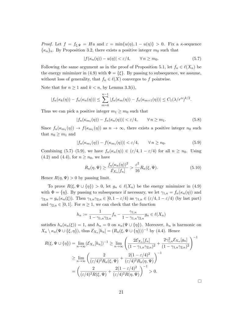
Example 6.3. Sierpinski gasket It is the self-similar set K generated by the maps

Si(ξ) = 12(ξ−ei−1)+ei−1 where e0 = 0 and ei, i = 1, . . . , N−1 are the standard basis

vectors in RN−1. It is a p.c.f. set with P = {1∞, 2∞, . . . , N∞}, and α = dimH K =logNlog 2 . For the λ-NRW (rα = 1

N ), the conductance is c(x,x−) = c(x,y) = (λN)−|x|

where x ∼h y. The critical exponent of Λα,β/22,2 is

β∗1 = β∗2 = β∗3 =log(N + 2)

log 2at λ =

1

N + 2.

(The critical exponent is known in [Jo].)

∆-Y

#

1 2

3

11 22

33

1n

2n

3n

12n−1

21n−1

13n−1

31n−1

32n−1

23n−1

3λ

2Rn−1

1n

∗2n

∗

3n

∗

Figure 4: Cutting in Sierpinski gasket, N = 3

28

We only prove the case N = 3, the other case is the same (the reader is also

advised to use N = 2 to get a clearer picture). By symmetry, it suffices to find the

resistance R(λ)(1∞, 2∞). We denote R(λ)n = R

(λ)n (1n, 2n) for short.

To estimate the upper bound, we delete the edges (ϑ, i), (ijk, jik), for i 6= j ∈ Σ,

k = 0, 1, . . . , n−2 in the subgraph of Xn (see Figure 4). Then we get a new subgraph

consisting of 3 copies of Xn−1 with 3 horizontal edges (ijn−1, jin−1), i 6= j ∈ Σ

at level n connecting them; we label these copies by 1, 2, 3 such that the copy i

contains the vertex in. Then apply the the ∆-Y transform to the three vertices in

Ai := {ijn−1 : j ∈ Σ} at the n-th level of each copy to get a starlike tree with

center in∗ , i ∈ Σ respectively. As the resistance between any pair of vertices in Aiequals 3λRn−1, it follows that the resistance between in∗ and a vertex in Ai in the

corresponding starlike tree is 3λ2 Rn−1. Moreover, between any pair in∗ , j

n∗ , i 6= j,

there is a 3-step path [in∗ , ijn−1, jin−1, jn∗ ]. Replacing these paths with resistors, we

get a triangle with vertices {in∗ : i ∈ Σ} and each side has resistance 3λRn−1 +(3λ)n.

By applying the monotonicity law and the series law,

R(λ)n ≤ R(1n, 1n∗ ) +R(1n∗ , 2

n∗ ) +R(2n∗ , 2

n)

=3λ

2R

(λ)n−1 +

2

3(3λR

(λ)n−1 + (3λ)n) +

3λ

2R

(λ)n−1

= 5λR(λ)n−1 + 2 · 3n−1λn.

Hence R(λ)(1∞, 2∞) = limn→∞R(λ)n = 0 for λ ∈ (0, 1

5). By Proposition 5.3 and

Theorem 5.4, we have β∗1 ≤ β∗3 ≤log 5log 2 .

To obtain the lower bound of the critical exponent, we need another technique.

We reassign the conductance on the n-th level of the subgraph Xn (n ≥ 1): for

µ > 0, let c(x,x−) = (3λ)−|x| for x ∈ Xn, and let

c(x,y) =

{(3λ)−|x|, if |x| < n,

µ−1(3λ)−n, if |x| = n,for x ∼h y ∈ Xn.

Denote the resistance between 1n and 2n with respect to the above c by R(λ,µ)n . Then

apply the generalized ∆-Y transforms to each triangle (x,x1,x2,x3) for x ∈ Jn−1,

and then replace each pair {x,x′} by a single x (see Figure 5 for N = 2 for a clearer

illustration; Figure 6 for N = 3 corresponds to the dotted box in Figure 5).

We have

R(λ,µ)n ≥ 2µ

µ+ 3(3λ)n +R

(λ,φ(µ))n−1 , (6.4)

where φ is given by the parallel resistance formula

φ(µ)−1 =

[3λ

(2µ

µ+ 3+ µ

)]−1

+ 1. (6.5)

29

∆-Y

Shorting

1 1

µ

∆-Y1

µ+2

µ

µ+2

µ

µ+2

x

x1 x2

x

x1 x2

x0

1 1

2λµ

11 1

φ(µ)

Figure 5: µ-parameter and shorting for N = 2

∆-Y Shorting

x

x1

x2

x3

x

x0

x1 x3

µ

µ+3

µ

µ+3

1

µ+3

1 1 1

µ µ

µ

µ+3

µ

µ+3

x

x1 x3

µ

x2

µ

µ+3

x2

µ

µ+3

Figure 6: µ-parameter and shorting for N = 3

The equation φ(µ) = µ has a solution µ ∈ (0, 1) if and only if λ > 15 . With such

fixed point µ, by (6.4), we have R(λ)(1∞, 2∞) ≥ limn→∞R(λ,µ)n ≥ R

(λ,µ)1 > 0. By

Theorem 5.7, we have log 5log 2 ≤ β

∗1 ≤ β∗3 , and completes the proof. 2

In the next example, we adjust the above method slightly for the new situation

with two different effective resistances of (i∞, j∞).

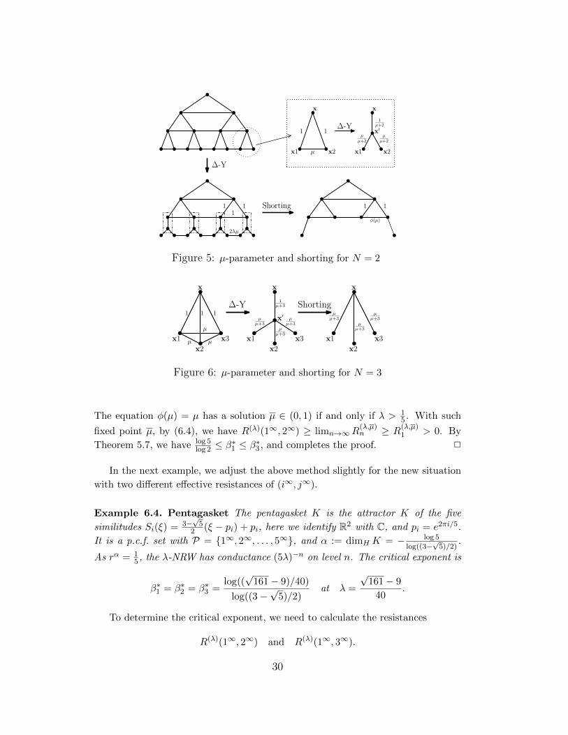
Example 6.4. Pentagasket The pentagasket K is the attractor K of the five

similitudes Si(ξ) = 3−√

52 (ξ − pi) + pi, here we identify R2 with C, and pi = e2πi/5.

It is a p.c.f. set with P = {1∞, 2∞, . . . , 5∞}, and α := dimH K = − log 5

log((3−√

5)/2).

As rα = 15 , the λ-NRW has conductance (5λ)−n on level n. The critical exponent is

β∗1 = β∗2 = β∗3 =log((

√161− 9)/40)

log((3−√

5)/2)at λ =

√161− 9

40.

To determine the critical exponent, we need to calculate the resistances

R(λ)(1∞, 2∞) and R(λ)(1∞, 3∞).

30

∆-Y

#

1 3

2

45

1n

5n

2n

4n

3n

1n

∗5n

∗

2n

∗

3n

∗

4n

∗

12n−1

15n−1

51n−1

54n−1

45n−1

43n−1

34n−1

32n−1

23n−1

21n−1

5λ

2(2An−1 −Bn−1)

5λ

2Bn−1

Figure 7: Cutting in pentagasket

We denote An = R(λ)n (1n, 3n) and Bn = R

(λ)n (1n, 2n) for short. By referring to

Figure 7, and using the same technique as before, we have

An ≤ R(1n, 1n∗ ) +R(1n∗ , 3n∗ ) +R(3n∗ , 3

n)

= 5λ(2An−1 −Bn−1) +[(10λBn−1 + 2(5λ)n)−1 + (15λBn−1 + 3(5λ)n)−1

]−1

= 10λAn−1 + λBn−1 +6

5(5λ)n.

Analogously, we have Bn ≤ 10λAn−1 − λBn + 45(5λ)n. As the coefficient matrix(

10λ λ

10λ −λ

)has eigenvalues 9±

√161

2 λ, we have limn→∞

An = limn→∞

Bn = 0 if λ <

(9+√

1612 )−1 =

√161−940 . Hence R(λ)(1∞, 2∞) = R(λ)(1∞, 3∞) = 0 for λ ∈ (0,

√161−940 ).

By Proposition 5.3 and Theorem 5.4, we have β∗1 ≤ β∗3 ≤log((

√161−9)/40)

log((3−√

5)/2).

To obtain the lower bound of the critical exponents, we reassign the conductance

on the bottom of the subgraph Xn (n ≥ 1) with two parameters µ1 and µ2 : for

µ1, µ2 ∈ (0, 1), let c(x,x−) = (5λ)−|x| for x ∈ Xn, and let

c(x,y) =

(5λ)−|x|, if |x| < n,

µ−11 (5λ)−n, if |x| = n and x− = y−,

µ−12 (5λ)−n, if |x| = n and x− 6= y−,

for x ∼h y ∈ Xn.

Denote the resistance between 1n and 3n (or 2n) with respect to above c by A(µ1,µ2)n

(or B(µ1,µ2)n ). We apply the local completion to each cone (x1,x11,x13,x14),

(x2,x22,x24,x25), (x3,x33,x35,x31), (x4,x44,x41,x42), (x5,x55,x52,x53) for

x ∈ Jn−2, and then replace each complete subgraph K4 by a starlike network with

greater energy (Figure 8). By a direct calculation, the conductance c∗ in K4 is given

by

c∗(x1,x11) =µ1 + 4

µ1 + 2, c∗(x1,x13) = c∗(x1,x14) =

µ1 + 3

µ1 + 2,

31

K4 Shorting

x11

x12

x13

x1

1 1 1

µ1 µ1

x15 x14

1 1

x11 x13

x1

x14x11 x13

x1

x14

ρ1ρ1

ρ2

Figure 8: Shorting in pentagasket

c∗(x11,x13) = c∗(x11,x14) =1

µ1(µ1 + 2), c∗(x13,x14) =

1

µ1,

and the resistances in the star are given by

ρ1 =µ1(µ1 + 2)

µ21 + 5µ1 + 5

, ρ2 =µ1(µ1 + 2)2

(µ1 + 1)(µ21 + 5µ1 + 5)

.

By the monotonicity law and series law,

A(µ1,µ2)n ≥ 2ρ2(5λ)n +A

(φ1(µ1,µ2),φ2(µ1,µ2))n−1 , (6.6)

(same inequality holds if we replace A by B) where φ1 and φ2 are given by the

parallel resistance formulas{φ1(µ1, µ2)−1 = [5λ (2ρ1 + µ2)]−1 + 1,

φ2(µ1, µ2)−1 = [5λ (2ρ2 + µ2)]−1 + 1.(6.7)

The equations φi(µ1, µ2) = µi, i = 1, 2 have a solution (µ1, µ2) ∈ (0, 1)2 if and only

if λ >√

161−940 . With such fixed point (µ1, µ2), by (6.6), we have R(λ)(1∞, 3∞) ≥

limn→∞A(µ1,µ2)n ≥ A

(µ1,µ2)1 > 0. Similarly we also have R(λ)(1∞, 2∞) > 0 if λ >

√161−940 . By Theorem 5.7, we have log((

√161−9)/40)

log((3−√

5)/2)≤ β∗1 ≤ β∗3 . 2

More computational issues on the critical exponent of nested fractals can be

found in [K]. Finally, we give an example that β∗1 6= β∗3 .

Example 6.5. Cantor set×interval Let Σ = {1, 2, 3, 4, 5, 6} and let p1 = 0, p2 =

(0, 13), p3 = (0, 2

3), p4 = (23 , 0), p5 = (2

3 ,13), p6 = (2

3 ,23) in R2. For i ∈ Σ, let Si(ξ) =

13ξ + pi on R2. Then the self-similar set K is the product of a Cantor middle-

third set and a unit interval (see the associated augmented tree in Figure 9), and

α = dimH K = log 2log 3 + 1 = log 6

log 3 . The λ-NRW has conductance (6λ)−n on the n-th

level (rα = 16). The critical exponents are

β∗1 = 2 at λ =1

9; β∗2 = β∗3 =∞

32

#

1 2 3 4 5 6

11 33

14 36

41

4466

63

Figure 9: The graph for Cantor set×inteval

First we show that R(λ)(1∞, 4∞) > 0 for any λ > 0. For n ≥ 1, consider a

function fn on Xn defined by

fn(x) =

1/2, if x = ϑ,

1, if i1 = 1, 2, 3,

0, if i1 = 4, 5, 6,

for x = i1i2 · · · ik ∈ Xn.

Then by (4.2), R(λ)n (1n, 4n) ≥ (EXn [fn])−1 = (6 · (1

2)2 · 16λ)−1 = 4λ. Thus for any

λ > 0, R(λ)(1∞, 4∞) = limn→∞R(λ)n (1n, 4n) ≥ 4λ > 0. By Theorem 5.4, we have

β∗3 =∞. Also it is easy to see that β∗2 =∞.

∆-Y

Shorting

∆-Y Shorting

x

x1 x2 x3

x

x0

x1 x3

µ

µ+1

µ

µ+1

1

µ2+4µ+3

1 1 1

µ µ

µ

µ+1

µ

µ+1

x

x1 x3

Figure 10: Shorting in Cantor set × interval

Next we consider the effective resistance R(λ)(1∞, 3∞) by using a similar short-

ing device as in previous examples. Denote R(λ)n = R

(λ)n (1n, 3n) for short. As in

Example 6.4, we reassign the conductance on the bottom of the subgraph Xn by an

additional factor µ−1, and by the same method applied to triangles (x,x1,x3) (also

to (x,x4,x6), see Figure 10), we have

R(λ,µ)n ≥ 2µ

µ+ 1(6λ)n +R

(λ,φ(µ))n−1 , (6.8)

33

where φ is given by

φ(µ)−1 = 2

[6λ

(2µ

µ+ 1+ µ

)]−1

+ 1. (6.9)

The equation φ(µ) = µ has a solution µ ∈ (0, 1) if and only if λ > 19 .

With such fixed point µ, by (6.8), we have R(λ)(1∞, 3∞) ≥ limn→∞R(λ,µ)n ≥

R(λ,µ)1 > 0. On the other hand, we show that if R(λ)(1∞, 3∞) > 0, then λ ≥ 1

9 .

Without loss of generality, we assume that 0 < λ < 1/6. For n ≥ 1, let fn be the

energy minimizer (harmonic function) on Xn with boundary conditions fn(1n) = 1

and fn(3n) = 0. Then Rn(1n, 3n) = EXn [fn]−1. By Corollary 5.2 (iv) ⇒ (iii), let

C1 := supn≥1 EXn [fn] = (infn≥1Rn(1n, 3n))−1 <∞. Pick a positive integer n1 such

that∑∞

n=n1+1(6λ)n < 136C1

. Then for n ≥ n1,

|fn(1n)− fn(1n1)|2 ≤ EXn [fn]RXn(1n, 1n1) ≤ C1

n∑k=n1+1

(6λ)k ≤ 1

36, (6.10)

which implies fn(1n1) ≥ 56 . Analogously we have fn(3n1) ≤ 1

6 . Let m = n − n1.

With a similar argument as in (6.10), for z ∈ {1, 4}m,

|fn(1n1z)− fn(1n1)|2 ≤ EXn [fn]RXn(1n1z, 1n1) ≤ 1

36,

which implies fn(1n1z) ≥ 23 . Analogously we have fn(3n1w) ≤ 1

3 for all w ∈ {3, 6}m.

Now, for z = i1i2 · · · im ∈ {1, 4}m, denote the word j1j2 · · · jm ∈ {3, 6}m with

jk = ik + 2 for all k by z′. Note that for each z ∈ {1, 4}m, there is a horizontal

path with length 3n − 1 from 1n1z to 3n1(z′). The resistance on such path is given

by RJn(1n1z, 3n1(z′)) = (3n − 1)(6λ)n. Counting the energy on these 2m disjoint

horizontal paths, we get

C1 ≥ EXn [fn] ≥∑

z∈{1,4}m

[fn(1n1z)− fn(3n1(z′))]2

RJn(1n1z, 3n1(z′))≥ 2n−n1

9(3n − 1)(6λ)n

for arbitrary n ≥ n1. Hence λ ≥ 19 and the claim follows. By Proposition 5.3, we

have β∗1 = 2. 2

Remark. To investigate the situation that β∗1 < β∗3 , it is natural to study the

products of self-similar sets. But in general, if K1 and K2 are connected self-similar

sets, then the critical exponent of the product K1 ×K2 satisfies

β∗1 ≤ max{dimH K1, dimH K2}+ 1 ≤ dimH K1 + dimH K2 = α.

34

Although the criteria in the last section cannot be applied directly, it still has a

similar link between the effective resistance of EX and the energy on the product

(see [K] for more details). For example, in the product [0, 1] × SG, the effective

resistances R(λ)(i∞, j∞) have two critical exponents λ∗1 = 14 and λ∗3 = 1

5 for various

i, j, while 2 = β∗1 <log 5log 2 = β∗3 < α = log 6

log 2 . With a similar technique as in Example

6.5, it follows that β∗1 = 2 if one of Ki is a unit interval. To generalize the results

above, we may leave a conjecture as

β∗1(K1×K2) = min{β∗1(K1), β∗1(K2)}, and β∗3(K1×K2) = max{β∗3(K1), β∗3(K2)}.

7 Remarks and open problems

The calculation of the critical exponents in Section 6 depends very much on the

p.c.f. property. It is challenging to find an effective technique to estimate the non-

p.c.f. sets like the Sierpinski carpet.

In our discussions, we assumed the return ratio λ ∈ (0, rα) (hence α < β∗1) in

order to guarantee functions in the domain of the induced bilinear form on K are

continuous (Proposition 2.5). While the condition is satisfied by the well-known

fractals, it also excludes the situation that β∗1 ≤ α, which contains important ex-

amples (e.g., the classical domain, and product of fractals). We conjecture that

the consideration in the paper is possible to adjust to this case. We also like to

know if there is a nice sufficient condition for α < β∗1 based on the geometry of the

self-similar sets.

We call a self-similar set K mono-critical if it has a single critical exponent

β∗ = β∗(K), i.e., β∗ = β∗1 = β∗2 = β∗3 . It is known that all nested fractals, Cantor-

type sets, and some non-p.c.f. sets including Sierpinski carpet (see [B, BB]) are

mono-critical. For these sets, the critical exponent plays an important role. It is

well-known that Λα,β∗/22,2 is trivial (see [Jo,P1]) while Λ

α,β∗/22,∞ admits a local regular

Dirichlet form on L2(K). On the other hand, it is constructed in [GuL] a modified

Vicsek set that is mono-critical; on this set, Λα,β∗/22,∞ is dense in L2(K, ν), but is not

dense in C(K), and there is a local regular Dirichlet form support by K which is

not Λα,β∗/22,∞ , and does not satisfy the energy self-similar identity [Ki1].

In conclusion, the question of constructing a local Dirichlet form on a self-similar

set is still unsettled. In view of the above, it will be very interesting to study this

situation in general, in particular, to use the return rate λ of the random walk to

study the boundary case.

35

Acknowledgements: The authors would like to thank Professors A. Grigoryan,

J.X. Hu and Dr. Q.S. Gu for many valuable discussions. They also thank Professor

S.M. Ngai for going through the manuscript carefully. Part of the work was carried

out while the second author was visiting the University of Pittsburgh, he is grateful

to Professors C. Lennard and J. Manfredi for the arrangement of the visit.

References

[An1] Ancona, A.: Negatively curved manifolds, elliptic operators, and the Mar-

tin boundary. Ann. Math. 125(1987), 495–536.

[An2] Ancona, A.: Positive harmonic functions and hyperbolicity. In: Potential

Theory: Surveys and Problems. Lecture Notes in Math. vol. 1344, pp.

1–23. Springer, Heidelberg (1988)

[B] Barlow, B.: Diffusions on fractals. Lecture Notes in Math. vol. 1690, pp.

1–121. Springer, Heidelberg (1998)

[BB] Barlow, M., Bass, R.: The construction of Brownian motion on the Sier-

pinski carpet. Ann. Inst. Henri Poincare 25(1989), 225–257.

[BeD] Beurling, A., Deny, J.: Espaces de Dirichlet. I. Le cas lmentaire. Acta

Mathematica, 99(1958), 203–224.

[CK] Chen, Z.Q., Kumagai, T.: Heat kernel estimates for stable-like processes

on d-sets. Stochastic Processes and their Applications 108(2003), 27–62.

[CKW1] Chen, Z.Q., Kumagai, T., Wang, J.: Stability of heat kernel estimates for

symmetric jump processes on metric measure spaces, arXiv:1604.04035

[CKW2] Chen, Z.Q., Kumagai, T., Wang, J.: Stability of parabolic Harnack in-

equalities for symmetric non-local Dirichlet forms, arXiv:1609.07594

[DS] Doyle, P., Snell, L.: Random walks and electric networks. The Carus Math.

Monogr. vol. 22 (1984)

[DL] Deng, Q.R., Lau,K.S.,: Open set condition and post-critically finite self-

similar sets. Nonlinearity, 21(2008), 1227–1232.

[Fa] Falconer, K.: Fractal Geometry: Mathematical Foundation and Applica-

tions. Wiley, New York (1990)

[FOT] Fukushima, M., Oshima, Y., Takeda, M.: Dirichlet forms and symmetric

Markov processes. De Gruyter Studies in Mathematics, vol. 19. Walter de

Gruyter & Co., Berlin (1994)

36

[GH1] Grigor’yan, A., Hu, J.X.: Off-diagonal upper estimates for the heat kernel

of the Dirichlet forms on metric spaces. Invent. Math. 174(2008), 81–126.

[GH2] Grigor’yan, A., Hu, J.X.: Upper bounds of heat kernels on doubling spaces,

Mosco Math. J., 14(2014), 505–563.

[GHH1] Grigor’yan, A., Hu, E.Y., Hu, J.X.: Lower estimates of heat kernels for

non-local Dirichlet forms on metric measure spaces (preprint)

[GHH2] Grigor’yan, A., Hu, E.Y., Hu, J.X.: Two-sided estimates of heat kernels

of jump type Dirichlet forms (preprint)

[GHL1] Grigor’yan, A., Hu, J.X., Lau, K.S.: Heat kernels on metric-measure

spaces and an application to semilinear elliptic equations. Trans. Amer.

Math. Soc. 355(2003), 2065–2095.

[GHL2] Grigor’yan, A., Hu, J.X., Lau, K.S.: Heat kernels on metric spaces. In:

Geometry and Anaysis of Fractals. Springer Proc. Math. Stat. vol. 88, pp.

147–207. Springer, Heidelberg (2014)

[GHL3] Grigor’yan, A., Hu, J.X., Lau, K.S.: Estimates of heat kernels for non-local

regular Dirichlet forms. Tran. Amer. Math. Soc. 366(2014), 6397–6441

[GHL4] Grigor’yan, A., Hu, J.X., Lau, K.S.: Generalized capacity, Harnack in-

equality and heat kernels of Dirichlet form on metric measure spaces, J.

Math. Soc. Japan 67(2015), 1–65.

[GuL] Gu, Q.S., Lau, K.S.: Dirichlet forms and critical exponents on post criti-

cally finite fractals (preprint)

[HK] Hu, J.X., Kumagai, T.: Nash-type inequalities and heat kernels for non-

local Dirichlet forms. Kyushu J. Math. 60(2006), 245–265.

[Jo] Jonsson, A.: Brownian motion on fractals and function spaces. Math. Zeit.

222(1996), 495–504

[Ka] Kaimanovich, V.: Random walks on Sierpinski graphs: hyperbolicity

and stochastic homogenization. Fractals in Graz 2001, Trends Math.,

Birkhuser, Basel, 145–183 (2003)

[Ki1] Kigami, J.: Analysis on Fractals. Cambridge Tracts in Mathematics vol.

143. Cambridge University Press, Cambridge (2001)

[Ki2] Kigami, J.: Dirichlet forms and associated heat kernels on the Cantor set

induced by random walks on trees. Adv. Math. 225(2010), 2674–2730.

[K] Kong, S.L.: Random walks and induced Dirichlet forms on self-similar

sets, PhD Thesis at The Chinese University of Hong Kong (2016)

[KLW] Kong, S.L., Lau, K.S., Wong, L.T.K.: Random walks and induced Dirich-

let forms on self-similar sets, arXiv:1604.05440

37

[Ku] Kumagai, T.: Estimates of transition densities for Brownian motion on

nested fractals. Probab. Theory Relat. Fields 96(1993), 205-224.

[LW1] Lau, K.S., Wang, X.Y.: Self-similar sets as hyperbolic boundaries. Indiana

Univ. Math. J. 58(2009), 1777–1795.

[LW2] Lau, K.S., Wang, X.Y.: On hyperbolic graphs induced by iterated function

systems. Adv. Math. (to appear)

[LP] Lyons, R., Peres, Y.: Probability on Trees and Networks (2011)

[P1] Pietruska-Paluba, K.: Some function spaces related to the brownian

motion on simple nested fractals. Stochastics and Stochastics Reports

67(1999), 267–285.

[P2] Pietruska-Paluba, K.: On function spaces related to fractional diffusions

on d-sets. Stochastics and Stochastics Reports 70(2000), 153–164

[Si] Silverstein, M: Classification of stable symmetric Markov chains. Indiana

Univ. Math. J. 24(1974), 29–77.

[St] Stos, A.: Symmetric α-stable processes on d-sets. Bull. Polish Acad. Sci.

Math. 48(2000), 237–245.

[Str] Strichartz, R.: Differential equations on fractals, a tutorial. Princeton

Univ. Press, Princeton (2006)

[TKV] Tetenov, A., Kamalutdinov, K., Vaulin, D: Self-similar Jordan arc which

do not satisfies OSC, arXiv:1512.00290

[Wo1] Woess, W.: Random Walks on Infinite Graphs and Groups. Cambridge

University Press, Cambridge (2000)

[Wo2] Woess, W.: Denumerable Markov Chains. European Math. Soc., Switzer-

land (2009)

Department of Mathematics, The Chinese University of Hong Kong, Hong Kong

slkong@math.cuhk.edu.hk

Department of Mathematics, The Chinese University of Hong Kong, Hong Kong

& School of Mathematics and Statistics, Central China Normal University, Wuhan,

430079, China.

kslau@math.cuhk.edu.hk

38