Shelf Management and Space Elasticity

Xavier DrèzeStephen J. Hoch

Mary E. Purk

Graduate School of BusinessThe University of Chicago

January 1994Revised July 1994

Last Revision November 1994

The authors would like to thank Dominick's Finer Foods, Information Resources Inc., andMarket Metrics for their assistance and provision of data. We also thank Bob Bycraft, Byung-DoKim, Alan Montgomery and Keyyup Lee for their help in analyzing the data. Special thanks toLinus Schrage for modifying LINGO to handle larger data sets.

Xavier Drèze is Director of MIS and a doctoral student, Stephen J. Hoch is Robert P. GwinnProfessor of Marketing and Behavioral Science, and Mary E. Purk is Manager of the Micro-Marketing Project, all at the University of Chicago.

Abstract

Shelf management is a difficult task in which rules of thumb rather than good theory and hard

evidence tend to guide practice. Through a series of field experiments, we measured the

effectiveness of two shelf management techniques: "space-to-movement", where we customized

shelf sets based on store-specific movement patterns; and "product reorganization" where we

manipulated product placement to facilitate cross-category merchandising or the ease of

shopping. We found modest gains (4%) in sales and profits from increased customization of

shelf sets and 5-6% changes due to shelf reorganization. Using the field experiment data, we

modeled the impact of shelf positioning and facing allocations on sales of individual items. We

found that location had a large impact on sales, whereas changes in the number of facings

allocated to a brand had much less impact as long as a minimum threshold (to avoid out-of-

stocks) was maintained.

3

Shelf Management and Space Elasticity

Introduction

Retailers can increase profits either by decreasing costs or increasing sales. The "cost

reduction" opportunities are of an operational nature --- they depend on efficient stock

management, personnel management, and exploiting technology. The "sales increase"

opportunities are market-driven, and can be divided in two categories: (a) out-of-store tactics and

(b) in-store-tactics. With out-of-store tactics the retailer works to bring more consumers into the

store, either by attracting new consumers or inducing current patrons to shop at their store versus

the competition more often. With in-store tactics the retailer attempts to extract more surplus

from consumers once they are in the store.

In this article, we focus on a subset of these in-store tactics. Specifically, we study how

retailers (and manufacturers) can boost sales by better managing existing shelf-space through

store-level shelf management, what is sometimes referred to as micro-merchandising. Instead of

relying on a single chain-wide policy, micro-merchandising involves the implementation of

store-specific merchandising and promotional tactics (Hoch, Kim, Montgomery, and Rossi

1995). Rapid developments in the efficient collection and analysis of sales data through UPC

scanners make it economically feasible to measure and monitor heterogeneity in local area

demand. The hope is that supermarket economies of scale and scope can be combined with the

customization that "Mom and Pop" stores offer in order to more effectively meet the wants and

needs of narrowly defined clienteles.

4

Indeed, one of the many challenges facing retailers is how to properly allocate shelf space

to the multitude of products they sell. A typical large supermarket carries more than 45,000

different items or stocking keeping units (sku’s) on an everyday basis. In 1992 there were 15,866

new grocery and health and beauty aid products introduced by manufacturers (Marketing News

1993). A typical chain may take on one-third of these new items each year. Each new product

adoption is accompanied with uncertainty regarding the most appropriate location for its display

and the optimal amount of shelf space to allocate.

Retail shelf space is valuable real estate. Store occupancy costs range from about

$20/square foot for dry grocery shelf space to over $50/sq ft for dairy and $70/sq ft for frozen

foods. Manufacturers expend considerable resources to secure this real estate: an improper

location or an under-allocation of space might kill a product before it achieves full sales

potential. And retailers work hard to maximize return on their investment: allocating too many

facings is a waste, while allocating too few will result in lost sales due to out of stocks.

Most manufacturers are willing to pay significant premiums to obtain preferred retail

locations on both a promotional and everyday basis. And retailers are more than willing to

accommodate manufacturers for the right price. Manufacturers spend 45-50% of their

promotional dollars on trade promotion, the vast majority used to secure feature advertising and

temporary display space in the form of front-walls, end-caps, wings, and in-aisle gondolas. In

many but not all product categories, retailers routinely charge slotting allowances when taking on

new products. Although these fees help to defray the costs of adding (and deleting) an item from

the system, they also cover the retailer’s opportunity costs for allocating shelf space to one item

over another. Some retailers supposedly even charge slotting fees to keep existing items on the

5

shelf. In specialty categories, manufacturers provide free display racks, for example Hartz

Mountain pet supplies, McCormick spices, and GE lighting. In exchange these manufacturers

obtain either exclusive or more prominent display privileges. In the cigarette category, all

manufacturers sign long term "rent" agreements for space. The "lead" manufacturer pays higher

rent and in return receives disproportionate shelf space.

The shelf space problem is quite different depending on whether we take the perspective

of the manufacturer or the retailer. Manufacturers want to maximize the sales and profits of their

products, and as such always want more and better space to be allocated to their brands.

Retailers want to maximize category sales and profits, regardless of brand identity; they must

allocate a fixed amount of shelf space in the best possible way.

After briefly reviewing prior research, we present the results of a series of shelf

management experiments. We analyze the effect of changes in shelf space and location on sales

and profits at two different levels: (a) the overall product category which is of greatest concern to

the retailer; and (b) individual brands which is primary to the manufacturer. We then utilize the

experimental data to parameterize a model that allows us to compute an upward bound on the

returns that might accrue to an "optimal" shelf set. We use this model to evaluate whether better

management of product location or product facings can provide greater returns to the retailer.

Why Should Shelf-Space Matter?

Although everyone agrees that shelf-space matters, the viability of micro-merchandising

depends on how much it really matters, that is the level of space elasticity. There are two distinct

ways in which changes in shelf space can affect category and/or brand performance. First,

changes in space influence the probability of an out-of-stocks. Clearly, the retailer cannot sell

6

something that is not in the store; this is a purely operational issue. We assume that store-level

micro-merchandising will decrease out-of-stocks to some degree because shelf space is more

closely allocated proportional to sales in comparison to a generic chain-wide shelf set. In the

field tests reported here, out-of-stocks did not appear to be a major problem because product

displays generally were quite large and the shelves usually were restocked at least once per day.

Second, changes in space can affect consumer attention; altering the visibility of a product

through changes in location or number facings should influence the probability of purchase. The

retailer potentially can improve performance by shifting consumers to higher margin items or by

increasing the number of unplanned purchases on a given shopping occasion.

Three characteristics of grocery shopping behavior suggest that consumer attention in the

store is both malleable and an important determinant of purchase behavior. First, the majority of

consumer decision making occurs in the store, suggesting that consumer information processing

is more bottom-up than top-down in nature (Hoch and Deighton 1989). Long-standing surveys

of supermarket shopping behavior have found that only about 1/3 of purchases are specifically

planned in advance of visiting the store (Dagnoli 1987). Second, consumers show a low level of

involvement with most of these in-store decisions, making choices very quickly after minimal

search (Hoyer 1984) and price comparison (Dickson and Sawyer 1990). This cursory level of

information processing suggests that simply increasing the salience of products through better

display could have significant effects on purchase behavior. Third, most consumers shop

multiple stores each and every week. The average shopper visits a supermarket 2.2 times a week

(Coca-Cola Research Council 1994). On average, however, shoppers visit each of their regular

7

supermarkets only 0.6 times a week. This means that, on average, consumers shop at 3 to 4

different supermarkets on a regular basis to satisfy their consumption needs.

In combination, these facts suggest that the total amount of dollars spent on any store visit

is quite discretionary and therefore an elastic quantity. The goal of any given retailer then is to

figure out how to increase the level of discretionary spending on each store visit; by doing so,

they will effectively increase their share of the shopper’s consumption requirements irrespective

of total consumer spending. For example, Milliman (1982) found that a decrease in the tempo of

background music slowed the pace of in-store traffic flow significantly. The slower pace in turn

resulted in substantial increases in per capita expenditures in the store.

Another way in which retailers can increase per capita transactions is by doing a better

job of attracting the consumer’s attention to additional purchase opportunities through numerous

temporary and permanent display characteristics. Clearly, temporary displays have the greatest

potential for attracting attention; their large size and novelty make them much more intrusive.

However, permanent displays can also be used to increase attention by manipulating: (a) the

location of the product within a display; (b) the area (facings) devoted to the product; (c) product

adjacencies; and (d) aesthetic elements such as size and color coordination and special signage.

Consider how permanent display could be used to influence two types of unplanned or impulse

purchases discussed by Stern (1962). Reminder purchases of frequently and habitually consumed

products are sparked when the consumer sees the product in the store. The best reminder for a

cigarette smoker is probably the package of their favorite brand; so when arranging the single-

pack cigarette fixture at the express check-out line, the retailer can maximize reminders across

consumers by placing the highest share brands in the most visible locations. Suggestion

8

purchases usually involve less frequently purchased products and so in-store merchandising must

provide a rationale for consumption. The suggestion factor can be increased by cross-

merchandising of natural complements: turkey’s and basters, white wine and fresh fish,

toothpaste and toothbrushes, or laundry detergent and fabric softener.

Although what we know about how consumers go shopping suggests that the returns to

increasing consumer attention are high, the question is how easy it is to manipulate attention

through better space management. The retailing environment is very noisy, with hundreds of

competing stimuli vying for attention. Our expectation going into the research was that it would

be difficult to increase salience in any significant way, so most changes in attention caused by

shelf management were likely to be small in magnitude.

Previous Space Management Research

Evidence on the sales impact of space management is limited because of the high costs of

implementing controlled experiments in the field. The existing work can be divided in three

types: commercial applications, experimental tests, and optimization models. The commercial

literature is composed of application oriented approaches where simplicity and ease of operation

are the most important features. In the PROGALY model (Malsagne 1972), for instance, space is

allocated in proportion to total sales. Cifrino (Chain Store Age 1963) and McKinsey (1963)

assign space in relation to Direct Product Profit (DPP). Other models have focused on

minimizing operating costs and reducing inventories and handling costs (Chain Store Age 1965).

Today there are numerous PC-based shelf management systems available to retailers including

Apollo (IRI) and Spaceman (Nielsen). Although each decision support system has

"optimization" capabilities with the input of space elasticities, in our experience retailers use

9

them mainly for planogram accounting purposes so as to reduce the amount of time spent on

manually manipulating the shelves.

A number of experiments have been conducted to measure shelf space elasticities, usually

focusing on a limited number of brands and only a few stores. An implicit assumption is that

there are diminishing returns from additional shelf space. Brown and Tucker (1961) postulated

three classes of products with respect to space changes: "unresponsive products", "general use

products", and "occasional purchase products". They showed that space elasticity increased as

one moved from one class to another. In the late 60’s and early 70’s, several controlled

experiments investigated the effect of changes in product facings on unit sales (Cox 1970;

Curhan 1972; Kotzan and Evanson 1969; Krueckenberg 1969). The average elasticity was about

0.2; that is, a doubling of facings led to a 20% increase in sales. Although this elasticity might

seem sizable to a manufacturer, it is not clear how significant it is to a retailer given the likely

within-category substitution that occurs.

Corstjens and Doyle (1981) focused on the optimization of shelf space for a chain of ice

cream and candy stores. They considered both the supply and demand side by taking into

account inventory and handling costs and own and cross space elasticities. Elasticities were

estimated using OLS, yielding a mean own elasticity of .086 and cross elasticity of -.028. An

interesting aspect of their work is that they do not constrain the interaction between categories to

be symmetric and some of the products are complements and some substitutes. A constrained

optimization indicated that profits can be increased from 3-20% depending on store size, though

these results were not empirically validated. Bultez and Naert (1988) use an attraction model to

represent the interaction between brands and apply it to space allocation for several product

10

categories in Belgian and Dutch supermarkets. The attraction model implies perfect substitution

between brands (a logical assumption since they work within rather than across categories); in

their model interactions are constrained to be symmetrical. As a result of their heuristic, each

item is allocated space proportional to market share and contribution to category profits. They

validate their work with some in-store implementations and find profit increases ranging from 6-

33%. Bultez et al. (1989) extend this work by utilizing an asymmetric attraction model and

incorporate multiple sizes of the same brand. Although progress slowly has been made, these

methods typically have considered only small subsets of brands; moreover, they have not taken

into account the position of each item.

Overview of the Experiments

The purpose of our experiments was to investigate the sales and profit potential of micro-

merchandising through better shelf-management. The tests were carried out at Dominick's Finer

Foods (DFF), a leading supermarket chain in Chicago. Two different types of shelf management

experiments were implemented: space to movement and product reorganization. In the space to

movement (STM) tests, product allocations were customized to meet historical sales in specific

demographic-based store clusters rather than the standard practice of a single chain-wide

allocation for each category. The various reorganization schemes revolved around two central

themes: complementary cross-merchandising and ease of shopping.

Sixty stores participated in the tests; each store was randomly assigned to a control or test

condition (separately for each category). There was a warm-up period of about 4 weeks after the

planogram changeover. The purpose of this period was to allow shoppers to become more

11

accustomed to the new shelf configuration, controlling for potential problems due to novelty,

confusion, or any other reaction.

Auditors from the Graduate School of Business at the University of Chicago monitored

the integrity of the planograms (spatial layouts of the category) bi-weekly. When problems arose

(e.g., misplaced products or incorrect number of facings), they worked with store personnel to

rectify the matter quickly. Both test and control planograms were monitored to eliminate

differences in neatness or maintenance between old (control) and new (test) shelf sets. In

general, when problems occurred, they happened early on after the reset (warm-up period).

Therefore, we are confident that the implementation was of high quality. During the test period,

changes in prices and promotions occurred as they would in the normal course of business.

12

Space-to-Movement Tests

Because it was not cost efficient to implement customized planograms for individual

stores, we clustered the stores based on geo-demographic data, the assumption being that stores

with similar customers would sell similar assortments of products. We performed a weighted k-

means cluster analysis based on the following variables (in order of importance): household size,

number of workers in family, household income, age of youngest child, race, home ownership,

education, marital status, adult age, employment status. The analysis yielded four clusters: inner-

city urban, blue collar urban, established suburbs, younger suburbs. These clusters form

concentric half circle radiating from Lake Michigan.

For each of the four clusters, we computed average unit movement over the last 12

months for each sku. Lack of distinctive movement patterns for each of the four clusters justified

a further reduction to two clusters of stores, one urban (22 stores) and one suburban (38 stores).

With this cluster level movement data, planograms were jointly designed by the manufacturers

and DFF using the Apollo and Spaceman decision support systems. As such, they represent

"good faith" efforts using state-of-the-art technology to produce improved shelf sets. The new

space to movement planograms resulted in: (a) increases and decreases in facings; (b) deletion of

slow moving items; (c) changes in shelf height; and (d) some changes in product positioning.

Allocating shelf space to movement (i.e., proportional to market share) decreases the probability

of out-of-stocks. Moreover, if we assume that the packages of products that people normally

purchase (the higher share items) are more likely to attract attention than those that they do not

regularly buy, it also effectively increases the level of attention across all consumers in a store.

13

All planograms retained their original size in term of lineal feet. In essence, the size of

the merchandising "box" remained constant - we manipulated only the assortment of items and

where they were located inside the box. Figure 1 shows schematics of the urban and suburban

planograms in the dish detergent. The main difference here was the increase in automatic dish

detergent in the suburban stores compared to the urban stores. The allocation of lineal footage at

the category level is by itself an important issue to retailers that would benefit from more

research. However, the costly logistic and operational side-effects (changing the size of one

planogram affects the size of adjacent category planograms), make it a difficult topic to study

with large scale experimentation.

Shelf Reorganization Tests

Shelf reorganizations took two forms. In the first series of tests, planograms were

rearranged to facilitate cross-category merchandising by increasing the proximity of natural

complement products. We implemented this strategy in two categories: oral care and laundry

care. In both categories, one subcategory is fully penetrated with an average interpurchase time

of about 2 months (toothpaste and detergent) whereas the complement either is not purchased as

frequently (4-6 months for toothbrushes) or has much lower penetration (65% for fabric

softener). Our goal here was to increase attention toward the less prominent subcategory at the

time of purchase of the primary product. Toothbrushes were moved from the top shelf (72 inches

above the floor) to a shelf that was at eye level (56 inches). The increased visibility of the

toothbrushes was expected to have a positive impact on sales, while the toothpaste items moved

to the upper shelf would suffer, but to a lesser extent since they were more likely to be a planned

purchase. Similarly, laundry care originally had been vertically blocked, moving horizontally

14

from liquid detergent to powder detergent to fabric softener. To enhance complementary

purchase, we placed 8-12 feet of softeners in between the liquid and powder detergents where it

was more likely to be noticed by buyers of both forms of detergent. This move was expected to

benefit softener without affecting sales of detergents.

In the second series of tests, we tried to manipulate the ease of shopping. For example, in

bath tissue we attempted to make it more difficult for consumers to make price comparisons. At

the time of the test, quantity discounts for buying large sizes (packages of 12-24 rolls) were not

substantial; in fact, smaller sizes (4 packs) often were cheaper because of more frequent

promotion. Products were arranged by brand (all Charmin sizes displayed together) in the

original planogram, facilitating intra-brand price comparisons. In the test, we reorganized the

planogram by package size; by doing so, consumers had to walk 12-16 feet to make intra-brand

price comparisons across sizes. In the ready-to-eat (RTE) cereal and condensed soup categories,

our intent was to make it easier to shop by organizing the brands in what we and the

manufacturers believed was a more logical fashion. Our thinking was that discretionary

purchases could be increased by reducing the number of times that consumers give up looking

for a particular brand or flavor variant. For condensed soup, where Campbell’s represented over

95% of the category, we organized the flavors alphabetically (as in the spice section) rather than

the quasi-random order characterizing the control set. For cereals, brands originally were

organized by manufacturer (i.e., a Kelloggs block, a General Mills block, etc...). In the test

planogram, brands were organized by three types of cereals - all family, kids, adult - and then

further organized into subtypes such as raisin brans, fruit flavors, high fiber. This resulted in

substantial changes in positions on the 50 lineal foot display.

15

Category-Level Results

We analyzed the effects of the experiments on both dollar sales and profits. Because

profit margins for sku's within a category usually are quite similar, the profit results mimic the

sales results. To simplify the presentation, we will focus our discussion on dollar sales except

where the two sets of results diverge.

For each product category, we compared average weekly sales during the test period to

sales in a pre-experimental baseline period. All sales, regular and promotional, were included in

our performance measures. Baselines were computed over historical periods spanning 86 to 99

weeks depending on the category. Each experimental period lasted 16 weeks. We selected 16

weeks to balance off dual concerns about obtaining stable, steady-state results, and the reality

that it would be difficult to maintain planogram integrity indefinitely, especially with the barrage

of new product introductions in some categories. The results, however, appear robust to the

exact length of the test (we were able to maintain planogram integrity for more than forty weeks

in some categories).

Space-to-Movement Results

Customized planograms were developed separately for urban and suburban stores. Half

of the urban (11) and half of the suburban (19) stores received the space-to-movement

planograms; the other 30 stores received a chain-wide control planogram. Changes in sales and

profits of the 30 space-to-movement test stores relative to the 30 stores in the chain-wide control

group are reported in Table 1. Random assignment within urban and within suburban stores was

carried out separately for each product category, meaning that any individual store had control

planograms in some categories and space-to-movement planograms in other categories.

16

As can be seen in the second column, six out of the eight categories experienced sales and

profit increases, all statistically significant. The other two categories, canned seafood and dish

detergent, experienced non-significant sales declines. The average increase of 3.9% may seem

small in the grand scheme of things, but it is important to keep in mind that these increases are

made up of full margin sales, not the low margins obtained with promotional deals. Moreover,

they represent long term incremental profits on a stable fixed cost base, and so constitute a more

substantial improvement than is at first apparent. For example, for the 86 store supermarket

chain in question, a 3% sales increase in a category generating sales of $2,000/week/store at a

25% gross profit margin would produce incremental profits of over $67,000 per annum. This

increase in profit is at least an order of magnitude greater than the direct labor costs (probably

less than $3,000/category) associated with designing the micro-market planograms. In-store

labor costs for micro-market planograms would not be much greater because the planograms

already are changed annually to accommodate all the new product introductions.

These sales increases for the STM planograms can also be compared to their respective

changes in space allocation induced by customization. The last column of Table 1 displays the

overall percentage difference in number of facings per sku between the urban and suburban

versions of the space-to-movement planograms. The control stores (based on a chain-wide

average) fell in between. These percentages were calculated as follows. For each sku we

computed the difference in facings between the urban and suburban planograms. We then

summed these differences across sku’s and divided by the total number of facings in the set, that

is:

% Change in facing 'Σ|Urbani & Suburbani|Total Category Facings

17

This measure only captures aggregate changes in facings, with no regard to any changes in

position. Keep in mind that the size of the planograms themselves remained unchanged. For

each facing that was added to one item, a facing was removed from another item. For instance,

the 22% difference between the urban and suburban planograms in the dish detergent category

(Figure 1) is in main part a result of different space allocation to liquid detergents (e.g. Palmolive

Green) versus automatic detergents (Cascade). In suburban stores, the space ratio of liquid to

automatic was 65:35 and in urban stores it was 80:20. These allocations reflect the difference in

market shares of liquid and automatic in the respective stores.

The level of customization varied dramatically by category, ranging from 17 to 46%.

There is no clear correspondence, however, between changes in space and changes in sales at the

category level. In the dish detergent category, the 22% change in facings had no significant

impact on sales volume.

In sum, our findings suggest that there are modest, but not trivial, gains to implementing

customized space-to-movement planograms. The results in Table 1 most likely provide a lower

bound on such gains because operational limitations constrained our store clustering scheme to

be consistent across all categories. In more recent implementations, the retailer has moved to a

category specific clustering of stores, where stores are grouped together based on historical data

specific to the category under question. This ensures a higher degree of planogram customization

because the store clusters are maximally different in terms of product movement for any

18

particular category. In a follow-up test for the frozen entree category, we observed an additional

2% improvement by utilizing a category specific clustering of stores.

Complementary Merchandising Results

The two categories involved in the complementary merchandising tests, oral care and

laundry care, experienced significant sales and profit increases as a result of the new shelf sets.

Moving toothbrushes to eye level increased sales of toothbrushes by 8% and resulted in no

change in toothpaste sales (See Table 2). The profit picture was even more encouraging because

toothbrushes sell at twice the gross margin of toothpaste. Overall category (brush and paste)

profits increased by 6% (p<.05). The laundry care category experienced a 5% increase in sales

and profits (p<.01) after placing fabric softener in between liquid and powder detergents.

Although our expectation was only that fabric softener would respond positively to the change in

location, all three subcategories benefitted from the merchandising change.

Ease of Shopping Results

In the bath tissue category we physically separated different size packages of the same

brand by about 12 feet in order to increase the difficulty of making price comparisons and

possibly increase sales of higher margin big sizes. This merchandising scheme produced a 5%

increase in category sales and profits compared to the brand blocked control planogram (p<.001).

These results held up for a period of about 10 months before new product introductions

necessitated a complete category reset.

Our intent with the RTE cereal "type" set and soup alphabetization was to organize items

in a more user-friendly manner. Both test planograms had a substantial impact on sales.

Alphabetizing soups decreased sales by 6% (See Table 2) and blocking different brands of

19

cereals by their respective subcategories rather than by manufacturer decreased sales by 5%.

Although it is possible that the shelf resets inadvertently confused consumers, we do not find this

a likely explanation; the sales declines held up for over 6 months, long enough for consumers to

learn the new scheme. Another possibility is that we made it too easy for consumers to find the

items they were looking for and consequently reduced browsing and impulse purchases. We

conducted in-aisle intercept interviews with 200 frequent shoppers in two control and two test

stores. Consumers displayed virtually no knowledge of how each category was organized. They

found both the control and test planograms confusing. Only about 10% of test store consumers

reported any awareness that the category had been rearranged six months previously. Sommer

and Aikens (1982) also found that consumers showed poor knowledge of product location in the

interior aisles of the store. These sparse verbal reports, however, may underestimate consumer

knowledge to the extent that shoppers possess store schemas in spatial as opposed to analytic

form. We conclude that category shelf organization can have a substantial impact on

performance but readily admit that we do not have an adequate explanation of these last two

tests.

Where Do the Increased Sales Come From?

A reasonable question to ask at this point is why category sales increased at all? Did the

altered planograms attract more customers into the Dominick’s stores at the expense of

competing stores? Did consumers increase their consumption of the category?

The answer to this question probably varies from one category to another, but it seems

reasonably clear to us that we did not increase store traffic. Our changes were made in-store,

without informing the public of the shelf manipulations. It is more likely that the increase in

20

sales generated by the test planograms comes from consumers purchasing a higher share of their

category requirements at Dominick’s rather than the competition. It is not that DFF was able to

steal consumers away from the competition with the new planograms, but it was able to increase

its share of the total shopping experience. For the most part, DFF achieved this by being a better

match to customers' immediate needs. Category expansion might, nevertheless, have occurred in

the toothbrushes and fabric softener categories since these two categories are not fully penetrated.

Brand-Level Space and Location Elasticity

Thus far we have analyzed the experiments at the category level and considered how shelf

reorganization and changes in assortment affect category sales and profits. These questions

clearly are of tantamount importance to the retailer. The manufacturer (especially the market

leader) also cares about category performance but is more concerned about understanding how

their individual brands react to horizontal and vertical changes in shelf position and the addition

or subtraction of facings. The category experiments, by virtue of injecting a substantial dose of

independent variation into the normal course of business, provide good data for measuring brand

level space and location elasticity.

To study the effect of shelf allocation on brand sales, we estimated a log-log model, using

log of unit sales as the dependent variable and two sets of independent variables to capture space

and location elasticity effects. We also included a set of control parameters.

Location Parameters

Retailers and manufacturers believe that brand location has an important impact on sales.

Eye-level often is seen as the best location. However, when pressed to be more specific about

what is meant by eye-level, we found that experts were referring to any one of several shelves

a4Xijk%a5Xijk2%a6Yijk%a7Yijk2

%a8Yijk3

A standard refrigeration case is L-shaped. Most of the shelves are vertically1

stacked in a fashion comparable to the rest of the store. The well is the bottom of theL. It is a special horizontal bin at the bottom of refrigeration cases, about 2 feet abovefloor level, where consumers must lift the product up rather than pull it off the shelf.

21

above the knees but below 6 1/2 feet. Manufacturers also profess preferences for particular

positions along the horizontal plane. Some believe the middle is the focal position, but others

prefer the edges in order to be first or last in the planogram. Since we lacked a complete theory

on how location affects sales, we elected to model location effects in a fashion flexible enough to

accommodate multiple phenomena that might vary by category.

The location of each sku was measured by the coordinates of the center of its facings

relative to the lower left corner of the display as shown in Figure 2. We integrated these

coordinates into the model using a polynomial function. We chose a second degree polynome for

the horizontal coordinates (X ). This formulation is flexible enough to model cases where theijk

optimal position is in the middle of the aisle as well as cases where the optimal position is on one

or both edges (entry points to the category). We chose a third degree polynome for the vertical

coordinates (Y ). The degree of the polynome is higher for the vertical dimension because we ijk

needed to accommodate special fixtures like the “well” in refrigerated categories. The results do1

not change materially if the vertical dimension is restricted to be quadratic. The location portion

of the model is:

(1)

Space Elasticity Parameters

o'αe &βe &k Area

22

We represented the amount of space allocated to an item by the actual cross-sectional area

occupied by the product. For example, if there are two facings of an item whose package

dimensions are 3" x 4", then it occupies a total space of 24 square inches. We experimented with

a number of other measures, like shelf capacity or number of facings, but these measures have

shortcomings. Capacity is more of an operational measure. It is important because of out of

stocks, but in a system where shelves are re-stocked virtually every day, out-of-stocks are not that

common. Number of facings is a good measure intuitively because it is easy to understand and

communicate, however it is quite item dependent. One facing for a big item will not have the

same effect as one facing for a small item. Holding constant other packaging factors, people are

much more likely to visually acquire larger sized targets/products (Salvendy 1987).

We modeled the effect of space on sales using the Gompertz growth model. It is S-

shaped, characterized by non linear parameters, and a flexible form because it is not symmetric

around the point of inflection. The general form of the Gompertz growth model is:

(2)

It implies decreasing space elasticity as allocated area increases. We experimented with other

models of the area effect, for example logarithmic models of width and height or total surface

area. On the basis of fit, it is difficult to justify one particular specification of area over another.

We settled on the Gompertz specification because it mixes well with the rest of model, yielding a

reasonable estimation procedure, and it exhibits the following two characteristics:

- Bounded unit sales: one can argue that there must be a level at which incremental space

allocations stop having an impact on consumers because they are unable to process the

change, if for no other reason than the additional space is outside the visual field. In the

log(o)'log(α)&βe &kArea

a9 e&k(Aijk

a0%a1iBi%a2jSj%a3log(Pijk)

23

extreme, imagine an entire store full of only one item. Clearly, there is a limit to how

much a one-item store can sell.

- Concave in the vicinity of the origin: this feature is desirable because if the function is

convex over its entire domain, then there would be no benefits to lumping together two

facings of the same product. One would always be better off displaying each facing in a

different part of the display. Conversely, if the function is concave near the origin, it will

only pay off to split the display when a large number of facings is involved. In such a

case it would make sense to sell the same item in more than one location in the store.

Multiple locations in the store undoubtedly result in increased item sales, e.g., end-of-

aisle promotional displays, but it is not a practice that retailers typically endorse on an

everyday basis, mainly for reasons of operational control.

Since we use a log-log model, we need to take the natural logarithm of sales (o):

(3)

Log(α) can be incorporated in the model's constant, the space elasticity portion of our model is:

(4)

Control Parameters

We included control parameters to account for the heterogeneity across brands and across

stores. Individual brands have different baseline sales and specific stores have different store

traffic. Hence, we have (in addition to the constant) a dummy for each brand (B ), one for eachi

store (S ), and a price coefficient (P ) to account for changes in price over time (within items):j ijk

(5)

log(Uijk )' a0 %a1i Bi %a2j Sj %a3 log(Pijk )%

a4 Xijk%a5 X2ijk %a6 Yijk%a7 Y

2ijk %a8 Y

3ijk %

a9 e&k(Aijk% εijk

24

where i is a brand index, j a store index and k a week index.

Complete Model

The complete formulation of our model comes from the merging of equations 2, 5 and 6:

(6)

The model accounts for: (a) heterogeneity across brands; (b) heterogeneity across stores; (c)

category level price elasticity; (d) variation in the amount of space allocated to each sku; and (e)

variation in the location of each sku. The model does not account for: heterogeneity in brand and

store level price elasticities; trends (seasonality, category expansion, ...); or packaging attributes

other than size. Moreover, we do not explicitly model interactions between brands, whether due

to relative positioning (two brands together or apart) or relative number of facings.

Description of the Brand Level Data

In addition to the sku level weekly scanner data for each of the 60 stores involved in the

previously described experiments, we used a set of planograms describing the position, the

number of facings, and the package dimensions of each sku. A pictorial representation appears

in Figure 1. Each category had multiple planograms. For analysis we selected a total of 32

weeks of data, 16 weeks before planograms were changed and 16 weeks after. Because we were

interested in understanding space elasticity for permanent display space, we removed all

25

promotional sales from the dataset. There were several reasons for this choice. First, promotion

sales are usually accompanied with special displays (gondola, end-cap, ...). In such cases we are

unable to determine whether an item was picked up from the temporary or the regular display

area. Second, promotions are usually accompanied by special signage, drawing attention to the

product and the promotion. This effect of the extra signage is different from the location and

facing effects we are after. Third, promotions are often accompanied with more frequent

restocking of the shelves. Promoted items in the refrigerated juice section are restocked up to

three times a day, while non-promoted items are restocked during the night. Fourth, we are

interested in steady-state consumer reactions to changes in everyday space allocations. We

should say, however, that for each of the categories we studied it does not make any difference

empirically whether we estimate the model with or without promotional sales. The substantive

conclusions are virtually identical.

We focused on 8 category data sets where we had complete planogram information,

ranging in size from 20,000 to 150,000 observations (mean=66,000). The average category

contained 115 items, from a low of 27 in bath tissue to a high of 235 in analgesics.

Empirical Results

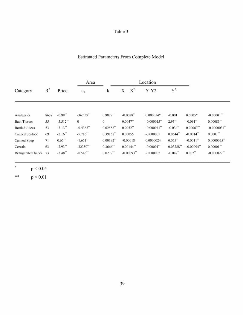
The model fits the data quite well (see Table 3). The average R was 67%, ranging from2

53% for bottled juices to 86% for analgesics. The order of importance of the variables was

consistent across categories. Based on the proportion of variance explained, the most important

determinants of sales were the brand and store dummies, followed by price and shelf location,

with area trailing behind. Since the control variables are not of direct interest, we focus our

discussion on location and area.

26

Location: Location was a statistically significant construct in all categories. On the horizontal

axis, there was no consensus on whether it is better to be located on the edges or in the center of

a set: half of the categories favored the edges, the other half favored the center (see the top half of

Figure 3). The results for the vertical dimension were more consistent. A central location is

most desirable, on average an elevation of 51-53 inches off the floor (see the bottom half of

Figure 3). This matches well with ergonomic research on the natural resting position of the eye.

The standard rule is that the preferred viewing angle lies 15 degrees below the horizontal

(Eastman Kodak Co. 1983). The average eye height for US females is 59” and for US males 64”.

If we assume that shoppers stand about four feet away from the shelves, this would imply

average resting positions of 49” and 55”. The one exception was in the refrigerated juice

category where the well was more valuable. Figure 4 displays the combined horizontal and

vertical effects for refrigerated juice.

Being statistically significant, however, is not enough. It also should be the case that the

impact of location on sales is large enough to matter to retailers and manufacturers. Using the

parameters estimated in the model, we found the best and worst positions (maxima and minima

of the polynome over the shelf domain) and then computed the expected differences in sales

between these two positions (see Table 4). We decomposed the location effect into its horizontal

and vertical components. By moving from the worst to the best horizontal position, a brand

could increase sales by 15% on average. In contrast, the difference between the worst and best

vertical position was 39% on average, more than 2.5 times the difference for horizontal location.

The combined effect resulted in a 59% increase. The largest horizontal effect occurs in the bath

tissue category. Canned soup showed no horizontal sensitivity, possibly because the planogram

27

was only 8 lineal feet. On the vertical dimension, cereals show tremendous sensitivity, possibly

due the important role that children play in the category.

One can question whether the position effect might be confounded with the brand effect

(i.e. the best brands are in the best positions and the small brands are out of sight). There are

three pieces of information that lead us to believe that this is not a problem. First, the model has

individual brand dummies. Hence, the position coefficients would be non-significant if position

and brands were confounded. Second, in the canned soup category, the biggest sellers were

located on the bottom shelves (for logistic purposes), and the model still estimated that location

to be the worse one. Last, in the refrigerated juices category, one test involved explicitly

switching the items in the well with the items on the second shelf. The effect measured matches

the model prediction.

Area: The area effect modeled through the Gompertz function was statistically significant

(p<.01) in all but one category. As for location, we must measure the actual economic impact of

area on sales. One way to look at this is to plot on the same graph the impact of area on sales,

and the current distribution of products across area. Figure 5 shows such a graph for analgesics.

The S-shaped line is the estimated Gompertz function. It shows that below 3 square

inches, sales potential is virtually non existent, and then increases sharply between 3 and 15

square inches, and levels off to full potential above 15 square inches. At 10 square inches of

display, a brand would reach about 98% of its potential. The histogram at the bottom of the

graph shows the distribution of items across the size of displays. About 2.5% of the items have

less then ten square inches of display, 12% have between 10 and 20 squares inches, and 85.5%

have more than 20 square inches (with 1% that have more than 150 square inches). As one can

28

see, most of the items have a number of facings that put them on the flat portion of the S curve,

indicating that adding or removing a facing would not affect their sale.

The situation represented in Figure 5 is characteristic of most of the other categories as

well. This suggests that in many situations manufacturers may receive a low return on

investment from their efforts to secure more shelf space. In fact, in these tests the return from

better shelf location was greater. Only in refrigerated juices and canned soups did we find a

situation where a significant portion of the items are on the upward segment of the Gompertz

function. In refrigerated juice (see Figure 6), more than 70% of the items had less than 150

square inches of display (beginning of the flat portion of the curve). Some of these items would

gain up to 50% in sales if they enjoyed more display space. In the canned soup category (See

Figure 7), there seemed to be an almost linear relationship between space and sales potential,

suggesting significant opportunities for improving performance. One possible explanation for

this linear relationship is that Campbell's dominates the category, and from a distance, all red and

white Campbell's cans look alike. Hence one has to read each label individually in order to find

the soup one desires, making the probability of being chosen directly proportional to a brand’s

space allocation.

Optimization of Space

In this section we attempt to utilize the empirically estimated parameters from our

experiments as input to an optimization routine. It was not our intention to develop a complete

model of shelf allocation and stock replenishment. Others, Bultez et al (1988) notably, have

produced detailed work in the area. Instead, we conducted this optimization exercise as a means

of better appreciating the upside potential of improved location and space allocations. We

29

attempted to build a reasonable facsimile of the consumer side of shelf management, and used

this model to better understand the potential of shelf management as a part of micro-marketing.

Optimizing shelf space allocations for our model is a difficult problem for which we do

not pretend to have a complete solution. In an ideal world, not only would we want to allocate

the appropriate amount of space and location to each item, we would also want to determine the

optimal number of shelves and the optimal height of each shelf given that a product can be

displayed on its side or turned upside down. The problem can be made easier to solve by

imposing a few reasonable assumptions.

We placed three restrictions on the space management problem. First, we decided

beforehand the number of shelves and shelf height. Second, we simplified the problem by

ignoring the horizontal position and assumed that only the vertical dimension matters. Last our

analysis ignores slotting allowances. The use of slotting allowances varies greatly across

categories and retailers. The reasons for the emergence of slotting allowances during the last

decade are not know with certainty (Sullivan 1994). It seems that except for categories with

exclusive distribution (e.g., greeting cards or spices) or rental arrangements (e.g., cigarettes),

there is no direct link between the acceptance of a new product by a retailer and the existence of a

slotting allowance (Rao and McLaughlin 1989). Retailers claim (Freeman 1991, Supermarket

News 1984) that slotting allowance are used to defray the administrative and logistic costs

associated with the introduction of new items rather than to buy a certain amount of shelf space.

In this light, we will carry out the rest of our analysis ignoring the existence of slotting

allowances. We acknowledge however that for categories such as those mentioned above,

slotting allowances could play an important role in planogram development.

Max Σi'1,N Profitijk(Usageijk

st: Σj'1,J Σk'1,K Usageijk '1 i'1,N

Σi'1,N Σj'1,J Usageijk(Sizeij ¸1 k'1,K

30

If we accept these three restrictions, the problem can be written as:

where: i is a item index (N items in the category)

j is the number of facings (maximum of j facings per item)

k is the shelf (K shelves)

Profit represents the profits accruing to j facings of item i if displayed on shelf kijk

Usage is 1 if item i is displayed on shelf k with j facings, and 0 otherwiseijk

Size indicates what proportion of the total width of the shelf is used in j facings of i areij

displayed on that shelf.

Because Profit is non linear in j and k, we first compute all possible Profit in advance andijk ijk

then feed the values into an optimization routine. Given that the sales matrix already exists, any

linear optimization package (LINDO, LINGO) is able to find the optimal solution in a reasonable

amount of time.

We ran this optimization on six categories analyzed in the previous section. Table 5

displays the results. The first column shows the expected improvement in profits for the optimal

shelf set compared to the existing planograms. The next two columns provide the profit

improvement that would be expected if we optimized either location or facings while holding the

other dimension constant. Specifically, to obtain an estimate of the profit improvement uniquely

attributable to optimal positioning of the products, we reran the optimization routine while

holding constant the allowable area allocated to each product. Each sku was allocated the exact

31

number of facings it had in the control planogram of our experiments. Similarly for area, we

optimized on facings while holding constant the shelf on which the product was displayed (the

control shelf).

In examining Table 5, we observe that in all cases the estimated category profit

improvement from the optimal shelf set is greater than that observed in our category experiments.

For example, while we observed a 2.6% increase in performance after moving to space-to-

movement planograms for refrigerated juice, expected profit from the optimal planogram is 8%.

A big part of this difference comes from the fact that we have calculated an optimal planogram

for each individual store, whereas in the experiment we were constrained to developing

planograms for only two clusters of stores. Because developing and maintaining individual

planograms is not operationally feasible for most retailers, our optimization results probable

represent an upward bound on the returns from better space management.

From the second and third columns of Table 5, we can see that in most of the categories

position optimization is more important than facing optimization. These category-level results

corroborate those found at the brand level, where we also found that location of the product was

more important than the number of facings. One difference between the results is the absolute

magnitude of the effects. For any individual brand, the improvement that accrues to better

location and more facings is much greater than when we look at the overall category. The reason

obviously is substitution. Only one brand can occupy any given position and similarly more

facings for one particular brand imply fewer facings for other brands.

This analysis highlights the tension between manufacturer and retailer goals mentioned at

the outset. Although manufacturers can experience substantial brand-level gains from securing

32

better shelf locations and modest gains from increased facings, the attendant category-level

benefits to the retailer are more modest. Thus it is crucial for both retailers and manufacturers to

consider the other party's interests when negotiating for space and location.

Conclusion

We found that a retailer can increase sales (and profits) by better managing existing shelf

space. We explored two different ways to increase profits: customized space-to-movement

planograms; and product reorganization intended to influence cross-merchandising and ease of

shopping. Each method produced different results. Customized space-to-movement led to

changes in sales and profits ranging from -2% to 8%, whereas product reorganization produced

changes in sales of 5-6%.

We then developed a model to measure the effect of changes in product location and shelf

space allocations on sales of individual brands within the category. On the whole, we found that

the majority of products were over allocated in terms of shelf space. Contrary to popular belief,

the number of facings allocated to a product was one of the least important success factors. A

product must, of course, be displayed in order to sell, but the return from additional shelf space

declined quickly, and above a certain threshold (different for each category), the benefits from

additional facings were non-existent. Position was far more important than the number of

facings. A couple of facings at eye level did more for a product than five facings on the bottom

shelf. Although there was no consensus about the best position on the horizontal axis (categories

were split evenly between the center of the aisle or the edges as being the best location), two

positions were clearly favored as far as the vertical axis is concerned: the well in the refrigerated

section; and slightly below eye level in the other categories.

33

After several years of shelf management experience, it is our belief that most supermarket

retailers should expect only modest gains in category sales, probably 4-5%, from better product

positioning and space allocation. This estimate represents only 1/3 of the 15% potential increase

suggested by our optimization results. There are several reasons why the retailer will not be able

to realize all this potential. First, they do not have the personnel to manage individual store

planograms in more than a handful of the 300 categories that they sell. Second, our optimization

is a static representation of a very dynamic world. With multiple new product introductions and

changes in demand for individual brands, sizes, flavors, and entire categories, the optimal shelf

set would be outdated before it could ever be implemented.

We do not mean to imply that there are no circumstances under which good shelf

management might not lead to more substantial sales gains. Our results come from only one

retailer at one point in time; moreover, most of the stores were large (>45,000 sq. ft). In the

U.K., by contrast, where land and building costs often are an order of magnitude greater than in

North America, supermarkets average about 1/3 the selling space per retail sales dollar. In such

cases where space is very tight, correct in-store inventory levels will be much more crucial to

avoid out-of-stocks and at the same time maintain reasonable restocking cycles. Similarly,

convenience stores, like 7-11, may observe a larger payback from improved shelf management.

It also should be kept in mind that our assessment of the value of shelf management

focused solely on the consumer demand side of the question. We took the size of a category

planogram and the general assortment of items as given, and then attempted to increase sales

through changes in brand-level product placements and space allocations. It is likely that there

are sizable gains on the operations side from "effective" shelf management. If the low space

34

elasticities that we encountered were to hold up, retailers could cut costs substantially by

reducing the overall space allocated to a category. Smaller category shelf sets would lead to

operational costs savings by reducing in-store inventories. By narrowing the assortment and/or

carrying fewer items, retailers could reduce administration and handling costs and simplify

warehouse inventory along the lines of the mass merchandisers and warehouse clubs. The freed-

up space could be allocated to new value-added services or non-traditional product categories

that might better benefit from the installed base of customers that currently traffic the store.

However, additional research is needed in this area because little or nothing is known about how

consumers would react to the cuts in breadth and depth of assortment that would accompany

shrinkage of the planograms.

35

References

Brown, W. and W. T. Tucker (1961), "The Marketing Center: Vanishing Shelf Space," AtlantaEconomic Review, (October), 9-13.

Bultez, A., E. Gijsbrechts, P. Naert, and P. Vanden Abeele (1989), “Asymmetric Cannibalismin Retail Assortments,” Journal of Retailing, 65 (2), 153-192.

Bultez, A., and P. Naert (1988), “S.H.A.R.P.: Shelf Allocation for Retailer's Profit,” MarketingScience, 7 (3), 211-231.

Chain Store Age (1963), "Cifrino's Space Yield Formula: A Breakthrough for Measuring ProductProfit," Vol. 39, No. 11.

Chain Store Age (1965), "Shelf Allocation Breakthrough," Vol. 41, No. 6.

Coca-Cola Retailing Research Council (1994), "Measured Marketing: A Tool to Shape FoodStore Strategy"

Corstjens, M., and P. Doyle (1981), “A Model for Optimizing Retail Space Allocations,”Management Science, 27 (7), 822-833.

Cox, K.K. (1970), “The Effect of Shelf Space upon Sales of Branded Products,” Journal ofMarketing Research, 7 (February), 55-58.

Curhan, R. (1972), “The Relationship between Shelf Space and Unit Sales,” Journal of MarketingResearch, 9(November),406-412.

Dagnoli, J. (1987), “Impulse Governs Shoppers,” Advertising Age, October 5, 93.

Dickson, Peter R., and Alan G. Sawyer (1990), “The Price Knowledge and Search ofSupermarket Shoppers,” Journal of Marketing, 54 (July), 42-53.

Eastman Kodak Co. (1983), Ergonomic Design for People at Work, New York: Van NorstrandReinhold Company.

36

Freeman, Laurie (1991), "Display Build Loyal Following: Change Seen in How SlottingAllowances Are Used," Advertising Age (May 6), p. 38.

Hoch, Stephen J., and John A. Deighton (1989), “Managing What Consumers Learn FromExperience,” Journal of Marketing, 53 (2), 1-20.

--------, Byung-Do Kim, Alan L. Montgomery, and Peter E. Rossi (1995), “Determinants ofStore-Level Price Elasticity,” Journal of Marketing Research, 32 (February), in press.

Hoyer, W.D. (1984), “An Examination of Consumer Decision Making for a Common RepeatPurchase Product,” Journal of Consumer Research, 11 (3), 822-831.

Kotzan, J. A., and R. U. Evanson (1969), “Responsiveness of Drug Store Sales to Shelf SpaceAllocations,” Journal of Marketing Research, 6 (November), 465-469.

Krueckenberg, H. F. (1969), “The Significance of Consumer Response to Display SpaceReallocation,” Proceedings of the Fall Conference, American Marketing Association, 30,336-339.

Malsagne, R. (1972), "La Productivité de la Surface de Vente Passe Maintenant par l'Ordinateur," Travail et Methodes, No. 274.

McKinsey-General Foods Study (1963), The Economics of Food Distributors. New York:General Foods.

Milliman, R.E. (1982), “Using Background Music to Affect the Behavior of SupermarketShoppers,” Journal of Marketing, 46 (3), 86-91.

Rao, Vithala and Edward McLaughlin (1989), "Modeling the Decision to Add New Products byChannel Intermediaries," Journal of Marketing, 53 (1), 80-88.

Salvendy, G. (1987), Handbook of Human Factors, New York: John Wiley and Sons.

Sommer, R., and S. Aikens (1982), “Mental Mapping of Two Supermarkets,” Journal ofConsumer Research, 9 (2), 211-215.

Stern, H. (1962), “The Significance of Impulse Buying Today,” Journal of Marketing, 26 (April),59-62.

Sullivan, Mary W. (1994), "What Caused Slotting Allowances?," The University of ChicagoWorking Paper.

37

Table 1

Space-to-Movement Results

Category Category Aggregate p valueChange in $ Sales Change in Facings

_______________________________________________________________________

Analgesics 8.4% 22% 0.0001

Bottled Juices 4.9 28 0.0001

Canned Soup 6.3 20 0.0001

Canned Seafood -1.0 45 0.09

Cigarettes 7.2 25 0.02

Dish Detergents -2.0 22 0.18

Frozen Entrees 4.4 22 0.0001

Refrigerated juices 2.6 19 0.0001

_______________________________________________________________________

Averages 3.9% 25%

38

Table 2

Ease of Shopping and Complementary Merchandising Results

Category Category Category Change in $ Sales p value Change in $ Profits p value

______________________________________________________________________________

Oral Care (Complementary)

Toothbrush 8% 0.05 11% 0.03

Toothpaste 1 0.06 1 0.15

Laundry Care (Complementary)

Detergent 4 0.005 4 0.007

Fabric Softener 3 0.01 3 0.01

Bath Tissue (By Size) 5 0.001 5 0.001

RTE Cereals (By Type) -5 0.08 -5 0.07

Canned Soup (Alphabetized) -6 0.002 -1 0.11

______________________________________________________________________________

39

Table 3

Estimated Parameters From Complete Model

Area Location

Category R Price a k X X Y Y2 Y2 2 39

__________________________________________________________________________________________

Analgesics 86% -0.98 -367.39 0.9827 -0.0028 0.000014* -0.001 0.0005* -0.00001** ** ** ** **

Bath Tissues 55 -5.512 0 0 0.0047 -0.000015 2.93 -0.091 0.00083** ** ** ** ** **

Bottled Juices 53 -3.13 -0.4363 0.02588 0.0052 -0.000041 -0.034 0.00067 -0.0000034** ** ** ** ** ** ** **

Canned Seafood 69 -2.16 -5.716 0.39158 0.00055 -0.000005 0.0544 -0.0014 0.0001** ** ** ** ** **

Canned Soup 71 0.65 -1.651 0.00192 -0.00018 0.0000024 0.055 -0.0011 0.0000075** ** ** ** ** **

Cereals 63 -2.93 -32350 0.3666 0.00144 -0.00001 0.03288 -0.00094 0.00001** ** ** ** ** ** ** **

Refrigerated Juices 73 -3.48 -0.543 0.0272 -0.00093 -0.000002 -0.047 0.002 -0.000027** ** ** ** ** ** **

__________________________________________________________________________________________

p < 0.05*

** p < 0.01

40

Table 4

Expected Increase in Brand-Level Sales When Moving from the Worst to the Best Location

Category Horizontal Vertical CombinedEffect Effect Effect

_____________________________________________________________________________

Analgesics 11% 19% 32%

Bath Tissues 52 18 79

Bottled Juices 27 41 79

Canned Seafood 3 54 59

Canned Soup 2 28 32

Cereals 5 100 112

Refrigerated Juices 22 69 108

_____________________________________________________________________________

Average 15% 39% 59%

41

Table 5

Increases in Profits When Optimizing on Both Area and Location,

Area Only, and Location Only

Category Both Area Location

______________________________________________________________________________

Analgesics 9% 1% 6%

Bottled Juices 25 1 20

Canned Seafood 15 1 12

Canned Soup 27 14 10

Oral Care 7 1 6

Refrigerated Juices 8 3 5

______________________________________________________________________________

Average 15% 3% 10%