Sheahen - Chirped Fourier Spec Part 1
6
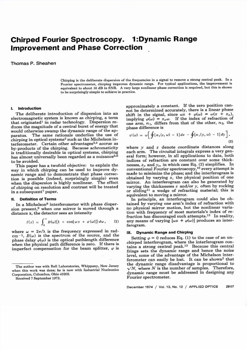
Chirped Fourier Spectroscopy. 1:Dynamic Range Improvement and Phase Correction Thomas P. Sheahen Chirping is the deliberate dispersion of the frequencies in a signal to remove a strong central peak. In a Fourier spectrometer, chirping improves dynamic range. For typical applications, the improvement is equivalent to about 16 dB in SNR. A very large nonlinear phase correction is required, but this is shown to be surprisingly simple to achieve in practice. 1. Introduction The deliberate introduction of dispersion into an electromagnetic system is known as chirping, a term that originated' in radar technology. Dispersion re- duces the magnitude of a central burst of energy that would otherwise swamp the dynamic range of the ap- paratus. The same rationale underlies the use of chirping in optical systems 2 such as the Michelson in- terferometer. Certain other advantages 3 4 accrue as by-products of the chirping. Because achromaticity is traditionally desirable in optical systems, chirping has almost universally been regarded as a nuisance 5 6 to be avoided. This paper has a twofold objective: to explain the way in which chirping can be used to improve dy- namic range and to demonstrate that phase correc- tion is possible (indeed, surprisingly simple) even when the dispersion is highly nonlinear. The effect of chirping on resolution and contrast will be treated in a subsequent 7 paper. II. Definition of Terms In a Michelson 8 interferometer with phase disper- sion present, 9 when one mirror is moved through a distance x, the detector sees an intensity I(x) = f B(w){1 + cos[cox + o(w)l}dw, (1) where w = 21r/X is the frequency expressed in rad- cm-1, B(w) is the spectrum of the source, and the phase delay s(w) is the optical pathlength difference when the physical path difference is zero. If there is imperfect compensation for the beam splitter, so s The author was with Bell Laboratories, Whippany, New Jersey when this work was done; he is now with Industrial Nucleonics Corporation, Columbus, Ohio 43202. Received 7 September 1973. approximately a constant. If the zero position can- not be determined accurately, there is a linear phase shift in the signal, since wx + so() = w(x + x 0 ), implying so(co) xow. If the index of refraction of one arm, n1, differs from that of the other, n2, the phase difference is cp w) w[ [n 2 (z,w) - 1]dz - n(y,w) - 1]dy], (2) where y and z denote coordinate distances along each arm. The circuital integrals express very gen- eral form; however, in all applications to date, both indices of refraction are constant over some thick- nesses, zo and yo, in which case Eq. (2) simplifies. In conventional Fourier spectroscopy,' 0 every attempt is made to minimize the phase; and the interferogram is obtained by varying x, the physical position of one mirror. An interferogram can also be generated by varying the thicknesses z and/or y, often by rocking or slidingl a wedge of refracting material; this is equivalent to moving a mirror. In principle, an interferogram could also be ob- tained by varying one arm's index of refraction with no physical mirror motion, but the nonlinear varia- tion with frequency of most materials's index of re- fraction has discouraged such attempts.' 2 In reality, any means of varying [ax + p(&))] roduces an inter- ferogram. 111. Dynamic Range and Chirping Setting so = 0 reduces Eq. (1) to the case of an un- chirped interferogram, where the con- tains a strong central peak.1 3 Because this central fringe sets the dynamic range and hence the noise level, some of the advantage of the Michelson inter- ferometer can easily be lost. It can be shown 2 that the dynamic range disadvantage is proportional to VN, where N is the number of samples. Therefore, dynamic range must be addressed in designing any Fourier spectrometer. December 1974 / Vol. 13 No. 12 / APPLIED OPTICS 2907
Transcript of Sheahen - Chirped Fourier Spec Part 1
8/11/2019 Sheahen - Chirped Fourier Spec Part 1
http://slidepdf.com/reader/full/sheahen-chirped-fourier-spec-part-1 1/6
Chirped
Fourier
Spectroscopy.
1:Dynamic
Range
Improvement
and
Phase
Correction
Thomas
P.
Sheahen
Chirping
is the
deliberate
dispersion
of
the
frequencies
in a
signal
to
remove
a strong
central
peak.
In a
Fourier
spectrometer,
chirping
improves
dynamic
range.
For
typical
applications,
the
improvement
is
equivalent
to
about
16 dB
in
SNR.
A very
large
nonlinear
phase
correction
is required,
but
this
is shown
to be surprisingly
simple
to
achieve
in
practice.
1. Introduction
The
deliberate
introduction
of dispersion
into an
electromagnetic
system
is
known
as
chirping,
a
term
that
originated'
in radar
technology.
Dispersion
re-
duces
the
magnitude
of
a central
burst
of
energy
that
would
otherwise
swamp
the
dynamic
range
of the
ap-
paratus.
The
same
rationale
underlies
the
use
of
chirping
in
optical
systems
2
such
as
the Michelson
in-
terferometer.
Certain
other
advantages
3 4
accrue
as
by-products
of the
chirping.
Because
achromaticity
is
traditionally
desirable
in optical
systems,
chirping
has
almost
universally
been
regarded
as
a nuisance
5 6
to be avoided.
This
paper
has
a
twofold
objective:
to
explain
the
way
in which
chirping
can
be
used
to
improve
dy-
namic
range
and
to
demonstrate
that
phase
correc-
tion
is
possible
(indeed,
surprisingly
simple)
even
when
the
dispersion
is
highly
nonlinear.
The
effect
of
chirping
on
resolution
and
contrast
will
be treated
in
a
subsequent
7
paper.
II.
Definition
of Terms
In
a
Michelson
8
interferometer
with
phase
disper-
sion
present,
9
when
one
mirror
is
moved
through
a
distance
x,
the
detector
sees
an
intensity
I(x)
=
f
B(w){1
+ cos[cox
+
o(w)l}dw,
(1)
where
w
=
21r/X
is
the
frequency
expressed
in
rad-
cm-1,
B(w)
is
the
spectrum
of
the
source,
and
the
phase
delay
s(w)
is the
optical
pathlength
difference
when
the
physical
path
difference
is zero.
If
there
is
imperfect
compensation
for
the
beam
splitter,
so
s
The
author
was
with
Bell
Laboratories,
Whippany,
New
Jersey
when this work was done; he is now with Industrial Nucleonics
Corporation,
Columbus,
Ohio
43202.
Received
7 September
1973.
approximately
a constant.
If
the
zero
position
can-
not
be determined
accurately,
there
is
a linear phase
shift
in
the
signal,
since
wx +
so()
= w(x
+
x
0
),
implying
so(co)
xow.
If
the
index
of
refraction
of
one
arm,
n1,
differs
from
that
of
the other,
n2,
the
phase
difference
is
cp w)
w[ [n
2
(z,w)
- 1]dz
-
n(y,w)
-
1]dy],
(2)
where
y and
z
denote
coordinate
distances
along
each
arm.
The
circuital
integrals
express
a
very
gen-
eral form;
however,
in all
applications
to
date,
both
indices of refraction are constant over some
thick-
nesses,
zo
and
yo,
in which
case
Eq. (2)
simplifies.
In
conventional
Fourier
spectroscopy,'
0
every
attempt
is
made
to
minimize
the phase;
and
the interferogram
is
obtained
by
varying
x,
the physical
position
of
one
mirror.
An interferogram
can also
be
generated
by
varying
the
thicknesses
z and/or
y, often
by
rocking
or slidingl
a
wedge
of
refracting
material;
this
is
equivalent
to
moving
a mirror.
In principle,
an
interferogram
could
also
be
ob-
tained
by
varying
one arm's
index
of
refraction
with
no
physical
mirror
motion,
but
the
nonlinear
varia-
tion
with
frequency
of
most
materials's
index
of
re-
fraction has discouraged such attempts.'
2
In reality,
any
means
of
varying
[ax
+ p(&))]
roduces
an
inter-
ferogram.
111.
Dynamic
Range
and
Chirping
Setting
so=
0 reduces
Eq.
(1)
to the
case
of
an
un-
chirped
interferogram,
where
the
interferogram
con-
tains
a strong
central
peak.1
3
Because
this
central
fringe
sets
the
dynamic
range
and
hence
the
noise
level,
some
of
the
advantage
of
the
Michelson
inter-
ferometer
can
easily
be
lost.
It can
be
shown
2
that
the
dynamic
range
disadvantage
is
proportional
to
VN, where N is the number of samples. Therefore,
dynamic
range
must
be
addressed
in designing
any
Fourier
spectrometer.
December
1974
/ Vol.
13
No.
12
/ APPLIED
OPTICS
2907
8/11/2019 Sheahen - Chirped Fourier Spec Part 1
http://slidepdf.com/reader/full/sheahen-chirped-fourier-spec-part-1 2/6
Analog
recording
of
interferograms
yields
unac-
ceptable
spectra,
as
we
have
displayed
elsewhere.'
4
This
difficulty
has
led the
commercial
market1
5
to di-
gitize
interferograms
in
real
time.
The
number
of
bits
and
the
digitization
rate
then
limit
the
speed
at
which
data can
be
acquired.
In
most
laboratory
applications,
the
source
is un-
changing
and
scanning
time is
not
at
a premium,
so
continuous
mirror
motion
is
not
mandatory. The
step-and-integrate
method
of
mirror
scanning
has
obtained
spectra
of
spectacular
quality,'
6
and
has
thus
gained
preeminence
for
high
resolution
work.
This method
allows
the
gain
state
to
be
switched
in
midscan;
and when
care
is
taken
to minimize
low
fre-
quency
drift,
it
is possible
to
circumvent
7
the
dy-
namic
range
problem.
Unfortunately,
discontinui-
ties
in
noise
level
introduce
coherent
structure
into
the
noise
spectrum.
Moreover,
if the
detector
begins
to
saturate
under
the intense
illumination
of
the
cen-
tral
peak,
false
harmonics
3
of
strong
lines
will
appear
in
the
spectrum.
Nevertheless,
if
step-and-integrate
methods were used throughout interferometry, dy-
namic
range
would
not
be
a serious
problem.'
7
There
remain
many
applications
of
Fourier
spec-
troscopy
where
data
acquisition
time
is limited.
Un-
fortunately,
even
fast servocontrolled'8
stepping
mechanisms
scan
much
more
slowly
than
the
contin-
uous
drive
method.
For
field
measurements
de-
manding
rapid
data
acquisition
in an unstable
envi-
ronment
(such
as the
remote
sensing
of air
pollutants
as
a
truck passes
a
sensor),
the continuous
scanning
method
is preferable.
This precludes
switching
of
gain
states,
making
dynamic
range
a problem
once
again.
A direct
method
of
mitigating
the
dynamic
range
problem
is
to
shrink the
central
fringe by
eliminating
the
common
point
of
zero path
difference
where
all
frequencies
can
add
constructively.
To achieve
this,
the
various
frequencies
are
deliberately
dispersed
by
introducing
frequency
dependent
delay
into
one arm,
called
chirping.
When
an
interferogram
(or any
electromagnetic
system)
is chirped,
there
is still
a
region
of construc-
tive
interference
among
neighboring
frequencies;
ut
nowhere
do
all
frequencies
add
in
phase.
As a re-
sult,
the
central
fringe
is dimmer,
and many
fringes
somewhat removed from the center are brighter.
The
total
power'
9
distributed
throughout
the
central
region
is preserved.
Typical
chirped
interferograms
have
already
appeared
elsewhere
2
1
4
; we
found
that a
-40
dB
chirped
interferogram
is
equivalent
to a
-56
dB unchirped
interferogram.
Chirping
generally
al-
leviates
the
dynamic
range
problem,
the
actual
im-
provement
depending
on the
degree
of
chirping
and
the
structure
of the
spectrum.
In unpublished
data,
Howell
et
a
2
0
have
shown
that
a blackbody
spec-
trum
improves
in
signal-to-noise
ratio
by
17
dB
when
chirping
is
introduced;
this
is
because
the unchirped
interferogram has a very strong central peak. At the
other
extreme,
a
pure
line
(e.g.,
a laser)
has
a
sinusoi-
dal
interferogram
regardless
of
chirping;
chirping
in-
troduces
delay
but
not
dispersion
and
offers
no
ad-
vantage
at all.
The
optimal
choice
of
chirping
material
depends
on the
particular
experiment.
For laboratory
appli-
cations,
it is
best
to have
a
selection
of
removable
and
interchangeable
dispersive
optical
elements
so
the
chirping
can
be changed
to
optimize
dynamic
range
as
the
character
of
the
spectrum
changes.
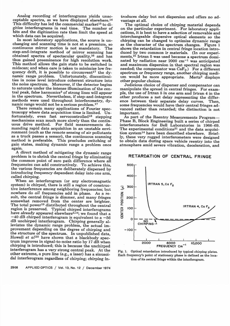
Figure
1
shows the retardation in central fringe location intro-
duced
by
two common
ir
materials.
(In
our
experi-
ments,
2
' Irtran
5
was used
because
a spectrum
domi-
nated
by
radiation
near
2000
cm'1
was anticipated
and
maximum
dispersion
in
that spectral
region
was
needed;
the compensator
was
CaF
2
.)
For
a different
spectrum
or
frequency
range,
another
chirping
medi-
um
would
be more
appropriate.
Mertz
2
displays
other
popular
choices.
Judicious
choice
of
disperser
and
compensator
can
manipulate
the spread
in
central
fringes.
For
exam-
ple,
the
use
of
Irtran
5
in
one
arm
and
Irtran
4 in the
other
produces
a
net
delay
representing
the differ-
ence between their separate delay curves. Then,
some
frequencies
would
have
their
central
fringes
ad-
vanced
rather
than
retarded;
the
distinction
is not
important.
As
part
of
the
Reentry
Measurements
Program-
Phase
B,
Block
Engineering
built
a
series
of
chirped
interferometers
for
Bell
Laboratories
in
1966-69.
The
experimental
conditions
2
' and
the
data
acquisi-
tion
system'
4
have
been
described
elsewhere.
Brief-
ly,
these
very
rugged
interferometers
were designed
to obtain
data
during
space
vehicle
reentry
into
the
atmosphere
amid
severe
vibration,
deceleration,
and
RETARDATION
OF
CENTRAL
FRINGE
500
400
300
_
I-
z
cn
0
.
CL
0
Z
w
I
IRTRAN
5 Ca
F
2
200 _
IRTRAN
100
_
14 Ca
F
2
0
-100
_
I
I
I
I
I
I
6000
FREQUENCY
Cm
1
10 000
000
Fig. 1. Optical retardation introduced by typical chirping plates.
Each
frequency's
point of
stationary
phase is
defined
as the
loca-
tion
of
its central
fringe
within
the
interferogram.
2908
APPLIED
OPTICS
/
Vol.
13
No. 12 /
December
1974
8/11/2019 Sheahen - Chirped Fourier Spec Part 1
http://slidepdf.com/reader/full/sheahen-chirped-fourier-spec-part-1 3/6
ORIGINAL
HIRPD
INTERFEROGRAM
I
I
I
I
000.4
0.06
0.0
-1.rII
II ..-
<
2
2<
00
2500
3000
TIME
SECI
3500
4000
4500
5000
5500
WAVE
NUMBER
RECONSTRUCTED
NCHIRPED
NTERFEROGRAM
I
I
I
TIME I
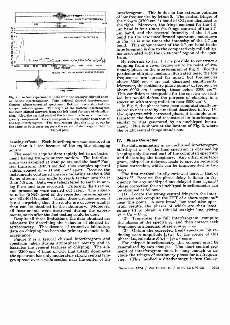
Fig.
2. Actual
experimental
data
from
the
strongly
chirped
chan-
nel of the interferometer. Top: original chirped interferogram.
Center:
phase
corrected
spectrum.
Bottom:
reconstructed
un-
chirped
interferogram.
The
origin
of the
bottom
interferogram
has
been
shifted
outward
from
the
left-hand
for
ease
of visualiza-
tion.
Also,
the
vertical
scale
of the
bottom
interferogram
has
been
greatly
compressed.
Its
central
peak
is
much
higher
than
that
of
the top
interferogram.
The
requirement
that
the
total
power
be
the
same
in
both
cases
suggests
the
extent
of
shrinkage
in
the
un-
chirped
plot.
heating
effects.
Each
interferogram
was
recorded
in
less
than
0.1 sec
because
of the
rapidly
changing
source,
The
need
to acquire
data
rapidly
led
to
an
instru-
ment
having
870-,m
mirror
motion.
The
interfero-
gram
was
sampled
at
2048
points
and
the
fast
2
2
Fou-
rier
transform
(FFT)
yielded
1024
complex
spectral
values,
spaced
Av
= 11.456
cm-'
apart.
Because
the
instruments
contained
mirrors
radiating
at
about
280
K,
no
attempt
was
made
to
reach
farther
into
the
ir
than
5.5
,im.
Data were
telemetered
to
earth
in ana-
log
form
and
tape
recorded.
Filtering,
digitization,
and
processing
were
carried
out
later.
The
signal-
to-noise
(SNR)
level
of
the
recorded
interferograms
was 40 dB
(1%
noise).
Under
these
circumstances,
it
is
not surprising
that
the
results
are of lower quality
than
can
be
obtained
in
the
laboratory.
Moreover,
all instruments
were
destroyed
during
the
experi-
ments,
so
no
after
the fact
testing
could
be
done.
Despite
all
these
limitations,
the
data
obtained
are
adequate
for
describing
the
behavior
of
chirped
in-
terferometry.
The
absence
of
extensive
laboratory
data
on
chirping
has been
the
primary
obstacle
to
its
acceptance.
Figure
2 is
a typical
chirped
interferogram
aiid
spectrum
taken
during
atmospheric
reentry
and
il-
lustrates
the
general
features
of
chirping.
The
4.3-
,m (2300-cm-') band of CO
2
that totally dominates
the
spectrum
has
only
moderately
strong
central
frin-
ges
spread
over
a
wide
section
near
the
center
of
the
interferogram.
This
is due
to the
extreme
chirping
of
low
frequencies
by
Irtran
5. The
central
fringes
of
the
2.7-gm
(3700
cm-')
band
of CO
2
are
displaced
to
the
right.
Moreover,
the
fringe
contrast
for
the
4.3-
,m
band
is
four
times
the fringe
contrast
of the
2.7-
,m
band,
and
the
spectral
intensity
of
the
4.3-gm
band
(in
the
raw
uncalibrated
spectrum,
not shown
in
Fig.
2)
is nine
times
the
intensity
of
the
2.7-,um
band.
This
enhancement
of the
2.7-gm
band
in
the
interferogram is due to the comparatively mild chirp-
ing
associated
with the
3700-cm-'
region
of
the
spec-
trum.
By
referring
to Fig.
1, it
is possible
to
construct
a
mapping
from
a
given
frequency
to
its
point
of sta-
tionary
phase
on the
interferogram
of Fig.
2.
For
the
particular
chirping
medium
illustrated
here,
the
low
frequencies
are
spread
far
apart;
but
frequencies
above
3500
cm1
are
not
dispersed
significantly.
Moreover,
the
stationary
phase
points
2
of frequencies
above
6000
cm-l
overlap
those
below 6000
cm-'.
This condition
is acceptable
for the
spectra
we
stud-
ied
but
would
defeat
the
purpose
of
chirping
in a
spectrum with strong radiation near 6000 cm-'.
In Fig.
2,
the
phases
have
been
computationally
re-
stored
to
near
zero
by
a method
described
in Sec.
IV.
Using
spectra
with
corrected
phase,
it is
simple
to re-
transform
the
data
and
reconstruct
an interferogram
similar
to that
generated
by an
unchirped
instru-
ment.
This
is shown
at
the
bottom
of Fig.
2,
where
the bright
central
fringe
stands out.
IV. Phase
Correction
For
data
originating
in an
unchirped
interferogram
starting at x = 0, the final spectrum is obtained by
keeping
only the
real
part
of the
computed
spectrum
and
discarding
the imaginary.
Any
other interfero-
gram,
chirped
or
delayed,
leads
to
spectra
requiring
phase
correction,
which
can
be
implemented
in
two
ways.
The
first
method,
briefly
reviewed
here,
is that
of
Mertz.
2 3
Because
the phase
delay
is linear
in
fre-
quency
for
any
unchirped
but
delayed
time
signal,
24
phase
correction
for an
unchirped
interferometer
can
be
obtained
as follows:
(1)
.Locate
the
strong
central
fringe
in
the
inter-
ferogram
and
compute
the FFT
of a
short
segment
2
3
near this point. A very broad, low resolution spec-
trum results,
the
phases
of which
are
then
least-
square
fit to obtain
a
fiducial
straight
line,
giving
of
= CO +
C W.
(2)
Transform
the
full interferogram,
compute
the
phases
of
the
spectra
(,g,
and
then
correct
each
frequency
to
a residual
phase
*
=
pg f.
(3)
Obtain
the corrected
(real)
spectrum
by
re-
ducing
each
amplitude
lg(w)l
by
the cosine
of
this
phase;
i.e.,
calculate
R
(w)
= Ig
w)I cos
or.
For
chirped
interferometry,
this
concept
must
be
generalized
by
two
changes.
The
short
central
seg-
ment of interferogram must be long enough to in-
clude
the fringes
of
stationary
phase
for
all
frequen-
cies.
(This
implied
a disadvantage
before
Cooley-
December
1974 /
Vol.
13
o. 12
/ APPLIED
OPTICS
2909
PHASE CORRECTED
PECTRUM
V.VL
I
I I
I
I
8/11/2019 Sheahen - Chirped Fourier Spec Part 1
http://slidepdf.com/reader/full/sheahen-chirped-fourier-spec-part-1 4/6
W
1
f
' '[' j -D '@
I
Z 8
-
M
6
2
0
2130
3000
4000
5000
6000
WAVE
NUMBER
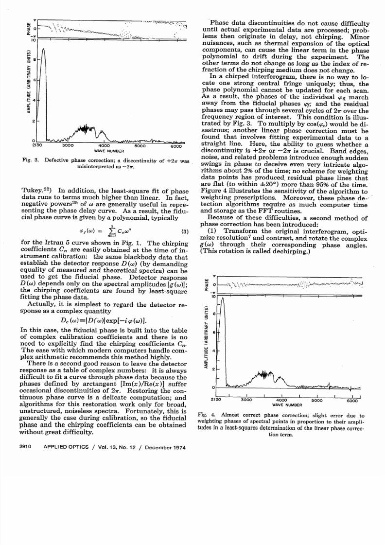
Fig.
3.
Defective
phase
correction;
a
discontinuity
of
+
2
7r was
misinterpreted as 27r.
Tukey.
2
2
)
In addition,
the
least-square
fit
of
phase
data
runs
to terms
much
higher
than
linear.
In fact,
negative
powers
25
of
are
generally
useful
in repre-
senting
the
phase
delay
curve.
As
a
result,
the
fidu-
cial
phase
curve
is
given
by
a polynomial,
typically
5
(Pf
()
CO,
(3)
n=-3
for
the Irtran
5
curve
shown
in
Fig.
1.
The
chirping
coefficients C are easily obtained at the time of in-
strument
calibration:
the
same
blackbody
data
that
establish
the
detector
response
D(cv)
(by
demanding
equality
of
measured
and
theoretical
spectra)
can
be
used
to
get
the
fiducial
phase.
Detector
response
D
()
depends
only
on
the
spectral
amplitudes
g
(c,)l;
the
chirping
coefficients
are
found
by
least-square
fitting
the
phase
data.
Actually,
it is simplest
to
regard
the
detector
re-
sponse
as a
complex
quantity
DC c)
|D(c)|exp[-iv(()].
In
this
case,
the
fiducial
phase
is
built
into
the table
of complex calibration coefficients and there is no
need
to explicitly
find
the chirping
coefficients
C.
The
ease
with
which
modern
computers
handle
com-
plex
arithmetic
recommends
this
method
highly.
There
is
a second
good reason
to
leave
the detector
response
as
a table
of
complex
numbers:
it
is
always
difficult
to fit a
curve
through
phase
data
because
the
phases
defined
by
arctangent
[Im(x)/Re(x)]
suffer
occasional
discontinuities
of
2
. Restoring
the
con-
tinuous
phase
curve
is
a
delicate
computation;
and
algorithms
for
this
restoration
work
only
for broad,
unstructured,
noiseless
spectra.
Fortunately,
this
is
generally the case during calibration, so the fiducial
phase
and
the
chirping
coefficients
can
be
obtained
without
great difficulty.
Phase
data
discontinuities
do
not
cause
difficulty
until
actual
experimental
data
are
processed;
prob-
lems
then
originate
in delay,
not
chirping.
Minor
nuisances,
such
as
thermal
expansion
of
the optical
components,
can
cause
the linear
term
in
the
phase
polynomial
to
drift
during
the
experiment.
The
other
terms
do
not
change
as
long
as the
index
of
re-
fraction
of the
chirping
medium
does
not
change.
In a
chirped
interferogram,
there
is
no
way
to
lo-
cate one strong central fringe uniquely; thus, the
phase
polynomial
cannot
be
updated
for each
scan.
As
a result,
the
phases
of
the
individual
og
march
away
from
the
fiducial
phases
so>;
and
the
residual
phases
may
pass
through
several
cycles
of 27r
over
the
frequency
region
of
interest.
This
condition
is illus-
trated
by
Fig.
3.
To
multiply
by
cos(p)
would
be
di-
sastrous;
another
linear
phase
correction
must
be
found
that
involves
fitting
experimental
data
to
a
straight
line.
Here,
the
ability
to
guess
whether
a
discontinuity
is +27r
or -2ir
is crucial.
Band
edges,
noise,
and related
problems
introduce
enough
sudden
swings
in
phase
to
deceive
even
very
intricate algo-rithms about
2%
of the
time;
no
scheme
for
weighting
data
points
has
produced.
residual
phase
lines
that
are flat
(to
within
20')
more
than
95%
of
the
time.
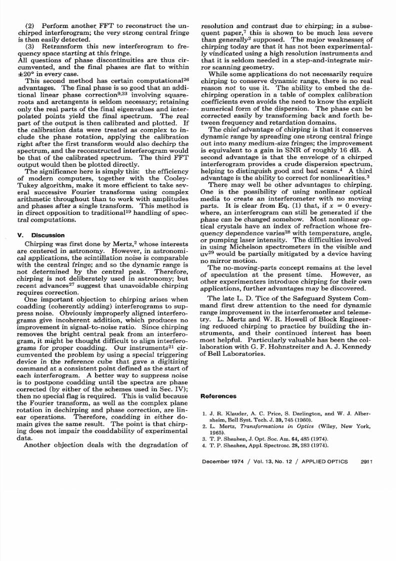
Figure
4
illustrates
the
sensitivity
of
the
algorithm
to
weighting
prescriptions.
Moreover,
these
phase
de--
tection
algorithms
require
as much
computer
time
and
storage
as
the
FFT routines.
Because
of
these
difficulties,
a
second
method
of
phase
correction
has
been
introduced:
(1)
Transform
the
original
interferogram,
opti-
mize
resolutions
and
contrast,
and
rotate
the complex
g (X)
through
their
corresponding
phase
angles.
(This rotation is called dechirping.)
to
I 0
a.
10
I
8
id
2130
3000
4000
5000
6000
WAVE
NUMBER
Fig.
4.
Almost
correct
phase
correction;
slight
error
due
to
weighting phases of spectral points in proportion to their ampli-
tudes
in
a least-squares
determination
of
the
linear
phase
correc-
tion
term.
2910
APPLIED
OPTICS
/ Vol.
13
No.
12 /
December
1974
8/11/2019 Sheahen - Chirped Fourier Spec Part 1
http://slidepdf.com/reader/full/sheahen-chirped-fourier-spec-part-1 5/6
(2) Perform another FFT to reconstruct the un-
chirped
interferogram;
the very
strong central fringe
is then
easily detected.
(3) Retransform this new interferogram to fre-
quency space starting
at this fringe.
All questions
of phase discontinuities
are thus
cir-
cumvented, and the
final phases
are flat to
within
L20
0
in every case.
This second
method
has certain computational
2
6
advantages. The final phase is so good that an addi-
tional linear phase correction '
23
involving square-
roots and
arctangents is
seldom necessary;
retaining
only
the real parts of the final eigenvalues and inter-
polated points yield the final spectrum. The real
part of the output is then calibrated and plotted. If
the calibration data were treated as complex to in-
clude the phase rotation,
applying the calibration
right after the first transform would also dechirp the
spectrum,
and the reconstructed
interferogram
would
be that of the calibrated spectrum. The third FFT
output would then be plotted directly.
The significance here is simply this: the efficiency
of modern computers, together
with the Cooley-
Tukey algorithm, make it more efficient to take sev-
eral successive Fourier transforms using complex
arithmetic throughout than to work with amplitudes
and phases after a single transform. This method is
in direct
opposition to traditional'
9
handling of spec-
tral computations.
V. Discussion
Chirping was first done by Mertz,
2
whose interests
are centered
in astronomy. However, in astronomi-
cal applications, the scintillation noise is comparable
with the
central fringe; and so the dynamic range is
not determined by the central peak. Therefore,
chirping is not deliberately used in astronomy; but
recent advances
27
suggest that unavoidable chirping
requires correction.
One important objection to chirping arises when
coadding (coherently adding) interferograms to sup-
press noise. Obviously improperly aligned interfero-
grams give incoherent addition, which produces no
improvement in signal-to-noise ratio. Since chirping
removes the bright central peak from an interfero-
gram, it might be thought difficult to align interfero-
grams for proper coadding. Our instruments
2 1
cir-
cumvented the problem by using a special triggering
device in the reference cube that gave a digitizing
command at a consistent point defined as the start of
each interferogram. A better way to suppress noise
is to postpone coadding until the spectra are phase
corrected (by either of the schemes used in Sec. IV);
then no special flag is required. This is valid because
the Fourier transform, as well as the complex plane
rotation in dechirping and phase correction, are lin-
ear operations. Therefore, coadding in either do-
main gives the same result. The point is that chirp-
ing does not impair the coaddability of experimental
data.
Another objection deals with the degradation of
resolution and contrast due to- chirping; in a subse-
quent paper,
7
this is shown to be much less severe
than generally
2
supposed. The
major weaknesses
of
chirping today are that it has not been experimental-
ly vindicated using a high resolution instruments and
that it is seldom needed in a step-and-integrate mir-
ror scanning geometry.
While some applications do not necessarily require
chirping
to conserve dynamic range, there is no real
reason not to use, it. The ability to embed the de-
chirping operation
in a table of
complex calibration
coefficients even avoids the need to know the explicit
numerical form of the dispersion. The phase can be
corrected easily by transforming back and forth be-
tween frequency and retardation domains.
The chief advantage of chirping is that it conserves
dynamic range by spreading one strong central fringe
out into many medium-size fringes; the improvement
is equivalent to a gain in SNR of roughly 16 dB. A
second advantage is that the envelope of a chirped
interferogram provides a crude dispersion spectrum,
helping to distinguish good and bad scans.
4
A third
advantage is the ability to correct for nonlinearities.
3
There may well be other advantages to chirping.
One is the possibility of using nonlinear optical
media to create an interferometer
with no moving
parts. It is clear from Eq. (1) that, if x
=
0 every-
where, an interferogram can still be generated if the
phase can be changed somehow. Most nonlinear op-
tical crystals have an index of refraction whose fre-
quency dependence varies
28
with temperature, angle,
or pumping
laser intensity. The difficulties
involved
in using Michelson spectrometers in the visible and
uv
29
would be partially mitigated by a device having
no mirror motion.
The no-moving-parts concept remains at the level
of speculation at the present time. However, as
other experimenters introduce chirping for their own
applications, further advantages may be discovered.
The late L. D. Tice of the Safeguard System Com-
mand first drew attention to the need for dynamic
range improvement in the interferometer and teleme-
try. L. Mertz and W. R. Howell of Block Engineer-
ing reduced chirping to practice by building the in-
struments, and their continued interest has been
most helpful. Particularly valuable has been the col-
laboration with G. F. Hohnstreiter and A. J. Kennedy
of Bell Laboratories.
References
1. J. R. Klauder, A. C. Price, S. Darlington, and W. J. Alber-
sheim, Bell Syst. Tech. J. 39, 745 (1960).
2. L. Mertz,
Transformations in Optics
(Wiley, New York,
1965).
3. T. P. Sheahen, J. Opt. Soc. Am. 64, 485 (1974).
4. T. P. Sheahen, Appl. Spectrosc. 28, 283 (1974).
December1974 / Vol. 13 No.12 / APPLIED OPTICS 2911
8/11/2019 Sheahen - Chirped Fourier Spec Part 1
http://slidepdf.com/reader/full/sheahen-chirped-fourier-spec-part-1 6/6
5. W. H. Steel,
Interferometry
(Cambridge U. P., Cambridge,
1967).
6. E. V. Loewenstein,
Aspen International Conference on Fouri-
er Spectroscopy, 1970;
Air Force Cambridge Research Labora-
tory Special Report 114 (5 January 1971), Ch. 1.
7. T. P. Sheahen, Chirped Fourier Spectroscopy. 2: Theory of
Resolution and Contrast (submitted to Appl. Opt.).
8. A. A. Michelson,
Light Waues and Their Uses
(Univ. of Chica-
go Press, Chicago, 1902, 1961).
9. M. L. Forman, W. H. Steel, and G. A. Vanasse, J. Opt. Soc.
Am. 56, 59 (1966).
10. J. Connes, Rev. Opt. 40, 45, 116, 171, 231 (1961).
11. P. Bouchareine and P. Connes,
J. Phys. Radium 24, 134
(1963).
12. Chirped interferometry must not be confused with amplitude
spectroscopy, which measures the index of refraction of an un-
known medium by observing the phase of the spectrum
pro-
duced by an interferometer containing the unknown in one
arm. See E. E. Bell, Ref. 6, Ch. 5.
13. G. A. Vanasse and H. Sakai, Progress in Optics, E. Wolf, ed.
(North Holland, Amsterdam, 1967), vol. 6, Ch. 7.
14. T. P. Sheahen, W. R. Howell, G. F. Hohnstreiter, and I. Cole-
man, Ref. 6, Ch. 25.
15. R. Curbelo and C. Foskett, Ref. 6, Ch. 21.
16. J. Connes, P. Connes, and J. P. Maillard, J. Phys. (Paris)
28C2, 120 (1967);
Atlas des Spectres Planetaires Infrarouges
(Editions du CNRS, Paris, 1969).
17. P. Connes, Ref. 6, Oh. 8.
18. J. E. Hoffman, Jr., Ref. 6, Ch. 15.
19. R. B. Blackman
and J. W. Tukey,
Measurement of Power
Spectra
(Dover, New York, 1959)
20. W. R. Howell, Digilab, Inc. (Cambridge, Mass.) private com-
munication.
21. G. F. Hohnstreiter, W. R. Howell, and T. P. Sheahen, Ref. 6,
Ch. 24.
22. J. W. Cooley and J. W. Tukey, Math. Comput, 19, 297 (1965).
23. L. Mertz,
Infrared Phys. 7,17 (1967).
24. R. Bracewell,
Fourier Transform and Its Applications
(McGraw-Hill,
New York, 1965).
25. I. Coleman and L. Mertz, Experimental
Study Program to In-
vestigate Limits in Fourier Spectroscopy,
Block Engineering,
Report AFCRL-68-0050(January 1968).
26. A convenience of FORTRAN IV evades the problem of shift-
ing each point in the reconstructed interferogram by a few
points. The data array is slightly overdimensioned (viz., 2060
locations for a 211 = 2048 point interferogram); and typically
the first ten points are repeated at the end. This is legitimate
since the unchirped interferogram is the FFT of 1024 complex
eigenvalues and is periodic over 2048 points. Then, if the cen-
tral fringe is found at location 7, the FFT subroutine is called
with the argument X(7). In this way, the change of an ad-
dress in the computer in effect performs a rotation in frequen-
cy space, showing a rather unexpected relationship between
computers and mathematical operations.
27. M. F. A'Hearn, F. J. Ahern, and D. M. Zipoy, Appl. Opt. 13,
1147 (1974).
28. A. Yariv,
Quantum Electronics (Wiley, New York, 1967).
29. A. S. Filler, Ref. 6, Ch. 42.
International Short Course in LASER-DOPPLERANEMOMETRY
in Karlsruhe Germany
An International Short Course on Laser-Doppler Anemometry will be presented
at the University of Karlsruhe in Germany. This course will take place
from 3rd March - 11th March 1975 and will be given in German and
Engl ish.
Each course is subdivided in two parts allowing time for detailed theore-
tical instructions and for experiments which will be carried out by the
participants themselves. During the theoretical part of the short course
each participant is allowed to use three out of six different commercial
instruments to carry out measurements in laminar and turbulent gas and
water flows as well as in diffusion and premixed flames.
For further details and program please write to
Sonderforschungsbereich 80
LDA - Short Course
University of Karlsruhe
D - 75 Karlsruhe 1, Kaiserstrafle 12
Germany
2912 APPLIED OPTICS / Vol. 13 No. 12 / December 1974