Shape Representation Using Space FilledSub-Voxel Distance Fields

M. W. Jones, R. A. SatherleyDepartment of Computer Science

University of Wales, SwanseaSingleton Park, Swansea

United Kingdomfm.w.jones, csrichg@swan.ac.uk

Abstract

Voxelisation is the process of converting a source objectof any data type into a three-dimensional grid of voxel val-ues. This voxel grid should represent the original object asclosely as possible, although some inaccuracies will occurdue to the discrete nature of the voxel grid representation.In this paper we report our on-going research into methodsfor representing objects as voxelised distance fields, in par-ticular we report fast methods for accurate distance fieldproduction. A review of current alternative voxelisationmethods is also given.

1 Introduction

The work presented in this paper is closely related to thefield of Volume Graphics [2]. Volume Graphics is an emerg-ing area of Computer Graphics which is concerned with theinput, storage, construction, modelling, analysis, manipu-lation, display and animation of spatial objects in a truethree-dimensional form. When comparing Volume Graph-ics to traditional surface graphics, the relationship has beenlikened to the relationship of that between two-dimensionalraster images and vector graphics [16]. The need for theprocess of voxelisation is a direct result of the employmentof volume graphics techniques, which in turn offer the ben-efits of scalable renderingalgorithms for extremely largescenes,visual effectssuch as fire, fur and roughness (Sec-tion 4.1) andconsistency of rendering(the ability to renderobjects of different source types under the same conditions).Indeed, as mentioned later in this paper, many rendering ef-fects are only available during volume rendering, and there-fore employing voxelisation techniques, enables these ef-fects to be carried out upon the voxelised objects.

In this paper we shall introduce distance fields in sec-

tion 2 and examine alternative methods for voxelisation insection 3. Section 4 will presentSpace Filled DistanceFields in detail. Binary segmentation and sub-voxel seg-mentation will be examined, and several methods for calcu-lating the complete distance field will be demonstrated. Fulldetails of the process for representing objects as distancefields will be given. Results will show how effective thesemethods are, including images and an animation (availablevia WWW site). Further work and conclusions are given insections 6 and 7.

2 Background

We have previously used distance fields as an intermedi-ate step to create triangular meshes from contour data [13].The use of the distance field helped avoid costly and dif-ficult point correspondence problems – particularly in 1 tomany and many to many branching cases. We discoveredearly on that the normals calculated from these distancefields (using trilinear interpolation within voxel cells) do notbecome quantised as they can with other methods, and thatsolid objects (obtained from contours or irregular points)can be represented quite accurately using this method. Wehave also used distance fields to voxelise triangular meshobjects [11]. That previous work described the productionof a shell distance field (also briefly reviewed in this paper),and an efficient algorithm for measuring the distance of apoint from a triangle (which is somewhat more difficult toachieve efficiently than one would assume). The work pre-sented here extends this previous work by generating space-filled distance fields efficiently, which as mentioned later inthis paper, have many more uses.

A distance fielddata setD representing a surfaceS isdefined as:D : R3 ! R and forp 2 R3 ,

D(p) = sgn(p) �min fjp� qj : q 2 Sg

sgn(p) =

��1 if p inside+1 if p outside

wherejj is the Euclidean norm

(1)

For each voxel in the three-dimensional grid, the distanceto the closest point on the surface is stored. Additionally,all voxels inside the object are set to be negative, and allvoxels outside are set to positive. This distance field haseffectively voxelised the object as the original surface canbe displayed by rendering the isosurface of level 0 fromD

- i.e. S = fq : D(q) = 0g whereq 2 R3 . Non-integer

grid points can be calculated from surrounding integer gridpoints using trilinear interpolation.

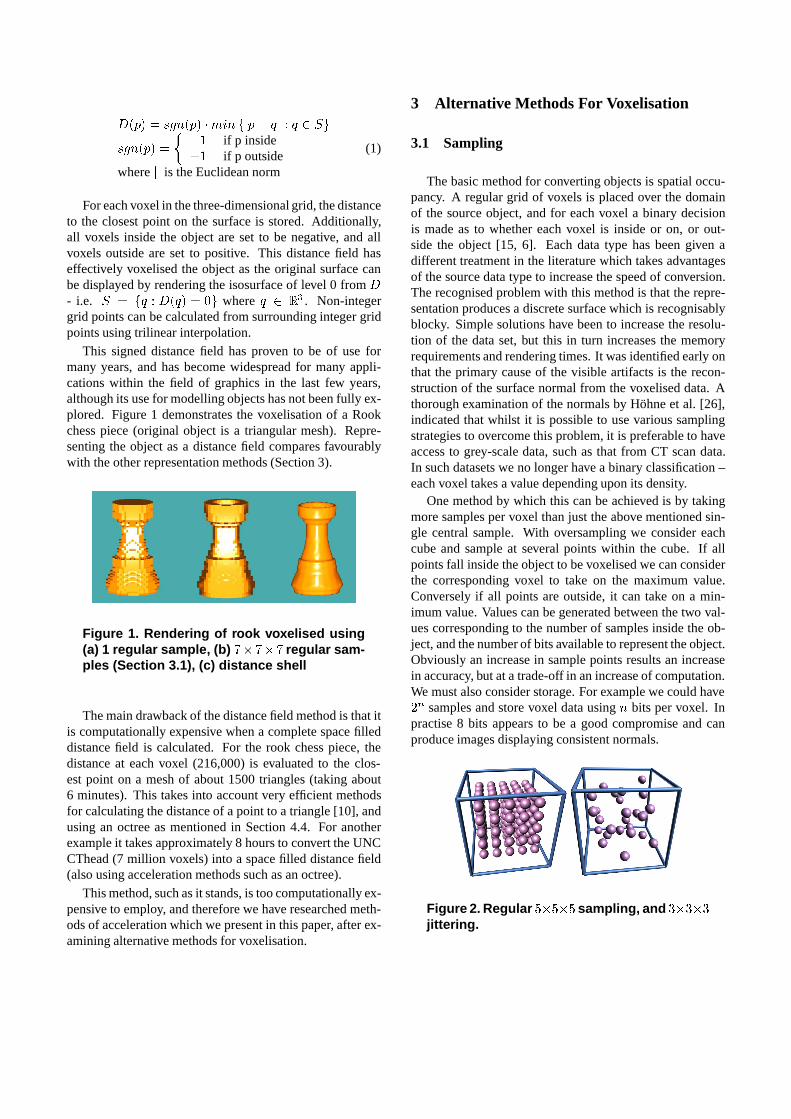
This signed distance field has proven to be of use formany years, and has become widespread for many appli-cations within the field of graphics in the last few years,although its use for modelling objects has not been fully ex-plored. Figure 1 demonstrates the voxelisation of a Rookchess piece (original object is a triangular mesh). Repre-senting the object as a distance field compares favourablywith the other representation methods (Section 3).

Figure 1. Rendering of rook voxelised using(a) 1 regular sample, (b) 7� 7� 7 regular sam-ples (Section 3.1), (c) distance shell

The main drawback of the distance field method is that itis computationally expensive when a complete space filleddistance field is calculated. For the rook chess piece, thedistance at each voxel (216,000) is evaluated to the clos-est point on a mesh of about 1500 triangles (taking about6 minutes). This takes into account very efficient methodsfor calculating the distance of a point to a triangle [10], andusing an octree as mentioned in Section 4.4. For anotherexample it takes approximately 8 hours to convert the UNCCThead (7 million voxels) into a space filled distance field(also using acceleration methods such as an octree).

This method, such as it stands, is too computationally ex-pensive to employ, and therefore we have researched meth-ods of acceleration which we present in this paper, after ex-amining alternative methods for voxelisation.

3 Alternative Methods For Voxelisation

3.1 Sampling

The basic method for converting objects is spatial occu-pancy. A regular grid of voxels is placed over the domainof the source object, and for each voxel a binary decisionis made as to whether each voxel is inside or on, or out-side the object [15, 6]. Each data type has been given adifferent treatment in the literature which takes advantagesof the source data type to increase the speed of conversion.The recognised problem with this method is that the repre-sentation produces a discrete surface which is recognisablyblocky. Simple solutions have been to increase the resolu-tion of the data set, but this in turn increases the memoryrequirements and rendering times. It was identified early onthat the primary cause of the visible artifacts is the recon-struction of the surface normal from the voxelised data. Athorough examination of the normals by H¨ohne et al. [26],indicated that whilst it is possible to use various samplingstrategies to overcome this problem, it is preferable to haveaccess to grey-scale data, such as that from CT scan data.In such datasets we no longer have a binary classification –each voxel takes a value depending upon its density.

One method by which this can be achieved is by takingmore samples per voxel than just the above mentioned sin-gle central sample. With oversampling we consider eachcube and sample at several points within the cube. If allpoints fall inside the object to be voxelised we can considerthe corresponding voxel to take on the maximum value.Conversely if all points are outside, it can take on a min-imum value. Values can be generated between the two val-ues corresponding to the number of samples inside the ob-ject, and the number of bits available to represent the object.Obviously an increase in sample points results an increasein accuracy, but at a trade-off in an increase of computation.We must also consider storage. For example we could have2n samples and store voxel data usingn bits per voxel. Inpractise 8 bits appears to be a good compromise and canproduce images displaying consistent normals.

Figure 2. Regular 5�5�5 sampling, and 3�3�3

jittering.

Sampling theory [28] suggests that a stochastic samplingshould provide better images as the high frequencies willbe dispersed. Poisson sampling using a minimum distanceconstraint (Poisson disk), such that no two points are closerthan a certain distance produces a good distribution for sam-pling but is expensive to calculate. In this instance the com-putational expense for calculating a Poisson disk for onecube and then using the same sampling pattern throughoutthe data set would be insignificant compared to the otheroperations. A simpler, but not much less effective method,is that of jittering (Figure 2). Each sample is randomly per-turbed from its centre on a regular grid, but is still locatedwithin its grid cell. This is simple to calculate (and imple-ment) as it just involves a random shift of the sample point.

Figure 3. Rendering of spheres using jittered(left column) and regular sampling (right col-umn). Samples per voxel (from top) 1, 8, 27,125, 9261.

Figure 3 shows an implementation of regular and jittersampling for the case of a sphere, and several samples pervoxel on a sampling grid of603. Table 1 gives the running

Samples per voxel time (secs.)1� 1� 1 0.022� 2� 2 0.133� 3� 3 0.455� 5� 5 2.12

21� 21� 21 222.31

Table 1. Computational time for various num-bers of samples per voxel ( 60�60�60 voxels)

times for each one (all timings are on an 800MHz Athlon).The artifacts apparent in the image are due to the grey-levelcentral difference method being used for the calculation ofthe normal. Only a 1 voxel layer encodes the surface – allother voxels are either completely inside the surface or com-pletely outside, and therefore there is not enough encodedinformation to reconstruct the normal accurately using thismethod. It is acknowledged that other methods exist forthis [26], but as it was not the main thrust of this work, theyhave been omitted.

We can observe that sampling within one slice of a gridof voxel values is similar to rendering the mesh to a pixelimage. Therefore we can accelerate the voxelisation processby using hardware renderers to render the triangular meshto an image. The image can then be processed to determineif each pixel was inside or outside the object. Fang [6] hascovered this process for point sampling, but this work couldbe easily extended to oversampling by simply increasing thesize of the image, and decreasing the stepping size throughthe volume. This is fine in the case of regular sampling, butjittering presents problems using this method.

Another method by which a grey-level dataset can becomputed is by using a different sampling technique. Wangand Kaufman [27] volume sample primitives using a spher-ical volume set at 3 units. Calculating this for arbitraryobjects (e.g. triangular meshes) is difficult, so they havespecific functions to volume sample each kind of primi-tive (sphere, cone etc.). The method produces values in thevicinity of the object, and therefore the volume is not spacefilled. This has advantages in terms of storage, but disad-vantages for applications mentioned in Section 4.1. Sr´amekand Kaufman [25] identify that a linear density profile in thevicinity of the surface give the best results. They producesuch a profile using convolution with a box filter. Againthis produces values in the vicinity of the object (whereasthis paper is primarily concerned with space filled voxeli-sations). Their method may benefit from the improvementsmade in this paper (as will become clear later). They sug-gest a method for voxelising surface represented objects inwhich the surface is voxelised using a field, such that a thinsolid is produced during visualisation – e.g. a plane would

become a box. Although the methods of Section 3.3 on-wards are discussed in the context of solid modelling, theycould be applied to surface representations in a similar man-ner (i.e. by creating slightly thick objects in place of in-finitely thin surfaces).

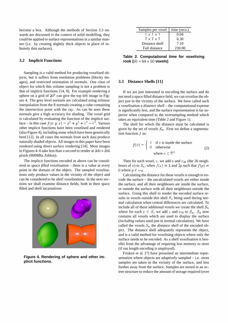
3.2 Implicit Functions

Sampling is a valid method for producing voxelised ob-jects, but it suffers from resolution problems (blocky im-ages), and restricted orientation of normals. One class ofobject for which this volume sampling is not a problem isthat of implicit functions [14, 8]. For example rendering asphere on a grid of203 can give the top left image in Fig-ure 4. The grey level normals are calculated using trilinearinterpolation from the 8 normals creating a cube containingthe intersection point with the ray. As can be seen thesenormals give a high accuracy for shading. The voxel gridis calculated by evaluating the function of the implicit sur-face – in this casef(x; y; z) = x2 + y2 + z2 � r2. Variousother implicit functions have been voxelised and rendered(also Figure 4), including some which have been geneticallybred [12]. In all cases the normals from such data producenaturally shaded objects. All images in this paper have beenrendered using direct surface rendering [14]. Most imagesin Figures 4–6 take less than a second to render at300�300

pixels (800Mhz Athlon).

The implicit functions encoded as above can be consid-ered asspace filledvoxelisation – there is a value at everypoint in the domain of the object. The sampled voxelisa-tions only produce values in the vicinity of the object andcan be considered to beshellvoxelisations. In the next sec-tions we shall examine distance fields, both in their spacefilled and shell incarnations.

Figure 4. Rendering of sphere and other im-plicit functions.

Samples per voxel time (secs.)1� 1� 1 0.047� 7� 7 6.30

Distance shell 7.10Full distance 230.00

Table 2. Computational time for voxelisingrook ( 60� 60� 60 voxels)

3.3 Distance Shells [11]

If we are just interested in encoding the surface and donot need a space filled distance field, we can voxelise the ob-ject just in the vicinity of the surface. We have called sucha voxelisation adistance shell– the computational expenseis significantly less, and the surface representation is far su-perior when compared to the oversampling method whichtakes an equivalent time (Table 2 and Figure 1).

The shell for which the distance must be calculated isgiven by the set of voxelsSn. First we define a segmenta-tion functionf as:

f(v) =

�1 if v is inside the surface0 otherwise

wherev 2 Z3

(2)

Then for each voxel,v, we addv andv26 (the 26 neigh-bours ofv) to Sv, whenf(v) = 1 and9p such thatf(p) =0 wherep 2 v26.

Calculating the distance for these voxels is enough to en-code the surface – the uncalculated voxels are either insidethe surface, and all their neighbours are inside the surface,or outside the surface with all their neighbours outside thesurface. Using this shell to render the encoded surface re-sults in voxels outside this shellSv being used during nor-mal calculation when central differences are calculated. Toinclude all of these additional voxels we create the shellSnwhere for eachv 2 Sv we addv andv26 to Sn. Sn nowcontains all voxels which are used to display the surface(including valuesused just in normal calculation). We havecalled the voxelsSn the distance shellof the encoded ob-ject. The distance shell adequately represents the object,and is a valid method for voxelising objects where only thesurface needs to be encoded. As a shell voxelisation it ben-efits from the advantage of requiring less memory to store(if run length encoding is employed).

Frisken et al. [7] have presented an intermediate repre-sentation where objects are adaptively sampled – i.e. moresamples are taken in the vicinity of the surface, and lessfurther away from the surface. Samples are stored in an oc-tree structure to reduce the amount of storage required (over

using a uniform grid). This representation will reduce cal-culation time (as less samples are made than a full distancefield), but will result in less accuracy away from the surface.Essentially their method is the same as a distance shell, withthe added benefit of less accurate distances available awayfrom the surface, rather than none at all as in the case of thedistance shell.

4 Space Filled Distance Fields

4.1 Overview

We have already demonstrated a simplistic approach tocalculating space-filled distance fields. Such distance fieldsoffer a powerful method by which objects can be repre-sented, manipulated and rendered. Animators are inter-ested in them for collision detection and morphing purposesand vision and image understanding researchers use themfor skeletonisation, thickening, thinning, shape interpola-tion and general distance calculations. An example of aspace-filled distance field for the rook is shown in Figure 5.At a distance of zero we have the original surface, and forvarious offsets we obtain the other surfaces as depicted.

Figure 5. Rendering of rook space filled dis-tance field at several different offsets.

It is now being appreciated that these distance fields havemany uses, such as:

� Skeletonisation – Danielsson [5], Paglieroni [19],Zhouet al. [31] and Zhou and Toga [32] use distanceinformation to extract the skeletal representation of anobject.

� Machine vision applications (Paglieroni [19]) – In-cluding, thickening, thinning, correlation, and conver-gence.

� General distance calculations – e.g. the calculation ofdistance to objects or contours and the production ofVoronoi tessellations.

� Shape-based interpolation (Levin [17] and Hermanetal. [9]) – Intermediate slices in scanned data can beinterpolated from distance information. Interpolation

from the original data causes abrupt changes at bound-ary locations.

� Distance field manipulation [20] – Distance informa-tion is added to surface models to allow their manipu-lation. Such manipulations include: interpolation be-tween two surface models, offset surfaces, blending oftwo surface, and surface blurring.

� Volume morphing – A morph between two distancevolumes can be easily created with the use of simplelinear interpolation [1], Figure 6 gives some imagesfrom such a morph. Cohen-Or et al. [4] use distancefields along with warp functions to create a morph be-tween two general topological objects.

Figure 6. Simple morph between a sphere anda CT skull.

Fig. 7 demonstrates the application of hypertexture todistance fields of triangular mesh objects and the UNCCThead.

� Accelerating ray tracing – Yagel and Shi [30], Cohenand Sheffer [3], and Semwal and Kvarnstrom [24] alluse CDT (see later) distance information to accelerateray tracing. The general principal behind each methodis to use the distance information to skip over largeempty spaces.

� Hypertextures (Satherley and Jones [23]) – Non-geometrically definable volume datasets, such as CTscans, can be converted to distance fields, allowing theapplication of Perlin and Hoffert’s hypertexture [21]effects, Figure 7.

All of the applications listed above require and use aspace-filled distance field. As it is so costly to computeaccurately, a faster (very inaccurate) propagation methodknown as adistance transform(DT) is used upon the bi-nary segmentation of the underlying object.

We will describe this basic method, and place it into con-text with other methods in our following classification. Asmany computer graphics researchers are using the simplemodel, the classification serves not only to demonstrate ourown methods, but also to bring other methods to a wideraudience.

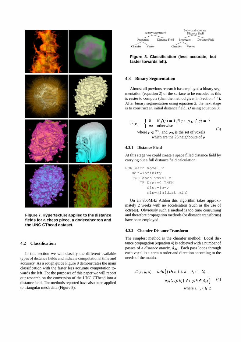
Figure 7. Hypertexture applied to the distancefields for a chess piece, a dodecahedron andthe UNC CThead dataset.

4.2 Classification

In this section we will classify the different availabletypes of distance fields and indicate computational time andaccuracy. As a rough guide Figure 8 demonstrates the mainclassification with the faster less accurate computation to-wards the left. For the purposes of this paper we will reportour research on the conversion of the UNC CThead into adistance field. The methods reported have also been appliedto triangular mesh data (Figure 5).

Binary Segmented Distance Shell

Propogate

Chamfer

Distance Field

Chamfer Vector

Distance Field

Vector

Sub-voxel accurate

Propogate

Figure 8. Classification (less accurate, butfaster towards left).

4.3 Binary Segmentation

Almost all previous research has employed a binary seg-mentation (equation 2) of the surface to be encoded as thisis easier to compute (than the method given in Section 4.4).After binary segmentation using equation 2, the next stageis to construct an initial distance field,D using equation 3:

D(p) =

�0 if f(p) = 1; 9 q 2 p26; f(q) = 0

1 otherwise

wherep 2 Z3; andp26 is the set of voxelswhich are the 26 neighbours ofp

(3)

4.3.1 Distance Field

At this stage we could create a space filled distance field bycarrying out a full distance field calculation:

FOR each voxel vmin=infinityFOR each voxel c

IF D(c)=0 THENdist=|c-v|min=min(dist,min)

On an 800MHz Athlon this algorithm takes approxi-mately 2 weeks with no acceleration (such as the use ofoctrees). Obviously such a method is too time consumingand therefore propagation methods (or distance transforms)have been employed.

4.3.2 Chamfer Distance Transform

The simplest method is the chamfer method: Local dis-tance propagation (equation 4) is achieved with a number ofpasses of adistance matrix, dM . Each pass loops througheach voxel in a certain order and direction according to theneeds of the matrix.

D(x; y; z) = min��D(x+ i; y + j; z + k)+

dM (i; j; k)�8 i; j; k 2 dM

�

wherei; j; k 2 Z

(4)

Chamfer distance transforms propagate local distance byaddition of known neighbourhood values obtained from thedistance matrix,dM , (an example of which is in Figure 9).Each value in the matrix represents the local distance value.This matrix is applied in two passes (and not recursivelypropagating one distance at a time as some authors havereported in previous work).

/* Forward Pass */FOR(z = 0; z < fz; z++)

FOR(y = 0; y < fy; y++)FOR(x = 0; x < fx; x++)D(x,y,z) = Eq.4

/* Backward Pass */FOR(z = fz-1; z � 0; z--)

FOR(y = fy-1; y � 0; y--)FOR(x = fx-1; x � 0; x--)D(x,y,z) = Eq.4

3

225

5 5

5

2

22

2

6

6

6

6 6

6

6

65

5 5

5

3 3

33

6

6

65

5

5

5

6

6 5 6

5

656

5 1

3 3

3 3

3

6 5 6

6326

5 2 2 5

63236

6 5 6

5 5

5225

1

1

3 3

1

3 3

3 3

3 3

33

3 3

0

1

1

3

3

3 3

3

3

3

Figure 9. Quasi-Euclidean 5 � 5 � 5 chamferdistance matrix.

The forward pass (using the matrix above and to the leftof the bold line, shown initalic font) calculates the dis-tances moving away from the surface towards the bottomof the dataset, with the backward pass (using the matrix be-low and to the right of the bold line) calculating the remain-ing distances. This method is computationally inexpensivesince each voxel is only considered twice, and its calcula-tion depends upon the addition of elements of the matrix toits neighbours.

This method of distance generation is very inaccurate,and hence all of the applications that rely on the methodare using inaccurate data. We required distance fields toproduce hypertextured objects, and we found that the bestdistance transforms did not produce accurate enough datafor the hypertexture to operate convincingly. This led us toinvestigate vector propagation methods.

4.3.3 Vector Distance Transforms (VDTs)

Vector methods [18] store a vector to the closest surfacepoint at each voxel. These vectors are propagated to neigh-bouring voxels in a prescribed way similar to the propaga-tion of distances via the distance matrix. Previous vectorpropagation methods operated on a binary segmented dataset (as in Equation 3), and so are attempting to produce adistance field from an object encoded as Figure 1(a).

VDTs generally require more passes of the distance ma-trix. During each pass the vector components are addedto the necessary vector position, the distance calculated, adecision made as to whether any of the new distances areminimal, and finally the minimal vector is stored.

To allow vector propagation Eqs. 3 and 4 are modified asshown in Eqs. 5 and 6 respectively.

~V (p) =

8><>:(0; 0; 0)

if p 2 S and

9 q 2 p26; q =2 S

(1;1;1) otherwise

(5)

D(p)=min��~V (x+i;y+j;z+k)+dM(i;j;k)

��8i; j; k 2 dM , wheredM = ( ~Mx; ~My; ~Mz)

(6)

Figure 10 shows the matrix passes employed by our Vec-tor City VDT.

4.4 Sub-Voxel Accurate Distance Field

The previous sections dealt with the left hand side ofour classification (Figure 8) and produce distance fieldswhich poorly approximate the underlying object. Ourmain contribution to this area is two-fold – firstly weuse our distance shellSv of Section 3.3 (Figure 1(c))as the starting point (although vectors to the closest sur-face point, rather than the distance to that point arestored), and secondly, we propagate distances using anew transform – the Vector City Vector Distance Trans-form (VCVDT). Complete details and analysis of themethod and its comparison to previous methods canbe found in our report [22] (available on http://www-compsci.swan.ac.uk/�csmark/voxelisation/). This paperdiffers from the report in the fact that it presents theVCVDT method as being applied to sub-voxel accurate dis-tances, contains information about using the method formodelling objects and is intended to present the results toa different audience.

Our method for modelling objects is to first calculatevectors for eachv 2 Sv (as defined in Section 3.3) to theclosest point on the surface. Fortriangular mesh objects,the closest point on the triangle is used. Computationaltime can be improved by using an octree to organise theobject – parts of the octree outside the current closest dis-tance can be ignored (thus reducing the number of trianglesto be considered for each voxel). A new voxel can use itsneighbours closest point as an initial starting point (so thatlarge amounts of the octree are ignored).

For CT data (or any other non-Euclidean grey-leveldata), 8 neighbouring voxels are considered to make a brickcell. A cell is transverse if at least one voxel is inside thesurface and at least one voxel is outside. For eachv 2 Sv

the closest transverse cells are stored in a list (again an oc-tree and neighbour information is used to speed computa-tion). Next, each transverse cube in the list is divided intotetrahedra, and then the closest point is calculated as theclosest point on the triangular tiling of the tetrahedra [20].This avoids the ambiguous cases present in marching cubes.The list of cells contains all cells that could contain the clos-est point – i.e. the furthest point in the closest cell is furtheraway than the closest point in the furthest cell.

The next stage uses this shell of voxelsSv about thesurface for which vectors to the closest point on the sur-face are known, and all other voxels in the domain are ini-tialised to a large value. We consider this voxel grid to be~V (p) 2 R

3 wherep 2 Z3. The vectors are now propa-

gated (using the VDT method) throughout the volume sothat equation 6 is true (D is the final distance field).

The matrix passes 8 times through the data set as shownin Figure 10 (our VCVDT), anddM is defined as the vectorvalues in Figure 10 (for further details see our report [22]).As an example though, the first forward pass F1 is appliedto each voxel in the direction of increasing x, y and z. Thenew vector at the voxel is the minimum of itself, its neg-ative y neighbour with -1 added to the y component of itsvector, and similar for its negative x and z neighbours. Thissmall example may seem to indicate no account is taken ofwhether we are moving away or towards the surface. In factlater passes (and the minimum operator) ensure that accountis taken. It may also make obvious the fact that the methodmay not give the correct closest voxel. This is true – themethod is an approximation, but as we shall see, it is about20 times more accurate than previous approximate methods.Figure 11 shows how the inaccuracies are introduced by themethod. The final distance is set to negative iff(v) = 1, orpositive iff(v) = 0.

(0,-1,0)

(1,0,0)

(0,1,0)(0,1,0)

y

x

y

x

y

x

z

z

z

B1B2

B4

(0,0,0)

y

x

z

B3

Forward Pass Backward Pass

F4

y

z

x

y

z

x

F2

y

z

x

F3

y

z

x

F1

(-1,0,0)

(0,0,-1) (0,-1,0)

(1,0,0)

(0,-1,0)

(0,0,1)

(0,1,0)

(1,0,0)

(0,1,0)

(1,0,0)(-1,0,0)

(0,-1,0)

(-1,0,0)

(-1,0,0)

Figure 10. Eight pass vector-city vector dis-tance transform.

correct vectorpropogated vectorcalculated vector

Figure 11. Incorrect vector propagation.

5 Results

Figure 12 shows several offset surfaces from the CT-head rendered from the distance field produced from thedistance shellSv using the above VCVDT vector trans-form. A full animation can be found at http://www-compsci.swan.ac.uk/�csmark/voxelisation/. The CTheaddistance shell (i.e. accurately measured sub-voxel distancesto the skull for allv 2 Sv) takes 240 secs. Table 3 showsthe additional time required to propagate these vectors (andcalculating the final distances), using our new VCVDTmethod, the current best method EVDT [18], and the CDTmethod, and compares this to the true calculation. It can beseen that for just over 4 minutes it is possible to compute thefull distance field to a good accuracy, rather than resortingto the 8 hour computation. Propagating the shell vectors forthe chess piece to create a complete distance field takes lessthan 2 seconds, and in fact Figure 5 was rendered from thepropagated rook distance field. We found that the field wasaccurate enough for our purposes (hypertexture – Figure 7),and the improved accuracy over the CDT method (currentlyused by most researchers requiring distances), would haveadvantages for all the applications mentioned earlier. Fig-ure 13 shows a volume graphics scene composed of distancefield encoded chess pieces and rendered using the volumerendering library – VLib [29].

6 Further Work

We are currently examining a hybrid technique using avector transform to direct the correct sub-voxel accurate cal-culation. We anticipate that this will fall between the cor-rect true calculation and transformed distance shell intermsof time. The distance field may be 100% accurate, althoughthis depends upon keeping a large list of candidates (Sec-tion 4.4, paragraph 3). We are also investigating other ap-plication areas not already identified in the literature.

7 Conclusions

We have introduced distance fields as a modellingparadigm and in particular introduced the notions of shelldistance fields and space-filled distance fields. Figure 1

Distance method Time Error range Avg errormin-max per voxel

True Euclidean 8 hrs 0.000–0.000 0.000000VCVDT 5.470s -0.334–0.334 0.000223

EVDT (previous best) 7.540s -0.518–2.533 0.004761CDT (3� 3� 3) 4.842s -0.415–11.769 2.196785

CDT (City Block–most common) 1.320 -2.00–76.060 12.269071

Table 3. Comparison of VCVDT with other methods

Figure 12. Rendering of CThead space filleddistance field at different isovalues (offsets).

demonstrated their superiority over sampling methods andtable 2 their comparable execution time for distance shells.Details for reproducing distance shells are given in 3.3and 4.4. A case for needing space-filled distance fields wasmade in Section 4.1, but computational expense was citedas a major problem. Section 4.4 builds upon the knowledgepresented in section 4.3 to demonstrate that vector meth-ods produce fairly accurate distance fields in less time. Ourcontribution to that area is a sub-voxel accurate segmenta-tion and a better vector transform, which we present in thispaper in relation to modelling objects.

We have demonstrated that distance fields can be usedto represent (voxelise) objects, but our overall aim was todemonstrate to the graphics community that fast,accuratespace filled distance fields can be calculated from distanceshells and thus become a realistic modelling paradigm withmany (already identified) application areas.

Acknowledgements

This work has been undertaken with funding from EP-SRC, UK, under grants GR/L88238 and GR/R11186.

Figure 13. A Volume Graphics scene usingsub-voxel accurate distance field encodedchess pieces.

References

[1] D. E. Breen, S. Mauch, and R. Whitaker. 3D scan conver-sion of CSG models into distance volumes. InProceedingsof the 1998 Symposium on Volume Visualization, ACM SIG-GRAPH, pages 7–14, October 1998.

[2] M. Chen, A. Kaufman, and R. Yagel, editors.VolumeGraphics. Springer-Verlag, 2000.

[3] D. Cohen and Z. Sheffer. Proximity clouds - an accelera-tion technique for 3D grid traversal.The Visual Computer,11:27–38, 1994.

[4] D. Cohen-Or, D. Levin, and A. Solomovici. Three-dimensional distance field metamorphosis.ACM Transac-tions on Graphics, 17(2):116–141, Apr. 1998.

[5] P.-E. Danielsson. Euclidean distance mapping.ComputerGraphics and Image Processing, 14:227–248, 1980.

[6] S. Fang and H. Chen. Hardware accelerated voxelisation. InVolume Graphics, pages 301–315. Springer, 2000.

[7] S. Frisken, R. N. Perry, A. P. Rockwood, and T. R. Jones.Adaptively sampled distance fields: A general representa-tion of shape for computer graphics. InSIGGRAPH Pro-ceedings on Computer Graphics, pages 249–254, July 2000.

[8] S. F. F. Gibson. Using distance maps for accurate surfacerepresentation in sample volumes. InProceedings of the1998 IEEE Symposium on Volume Visualization, pages 23–30, Oct. 1998.

[9] G. T. Herman, J. Zheng, and C. A. Bucholtz. Shape-basedinterpolation. IEEE Computer Graphics and Applications,12(3):69–79, May 1992.

[10] M. W. Jones. 3D distance from a point to a triangle. Tech-nical Report CSR-5-95, Department of Computer Science,University of Wales, Swansea, February 1995.

[11] M. W. Jones. The production of volume data from triangu-lar meshes using voxelisation.Computer Graphics Forum,15(5):311–318, December 1996.

[12] M. W. Jones. Direct surface rendering of general and ge-netically bred implicit surfaces. InProceedings of 17th An-nual Conference of Eurographics (UK Chapter) Cambridge,pages 37–46, April 1999.

[13] M. W. Jones and M. Chen. A new approach to the con-struction of surfaces from contour data.Computer GraphicsForum, 13(3):C–75–C–84, September 1994.

[14] M. W. Jones and M. Chen. Fast cutting operations on threedimensional volume datasets. InVisualization in ScientificComputing, pages 1–8. Springer-Verlag, Wien New York,January 1995.

[15] A. Kaufman. An algorithm for 3D scan-conversion of poly-gons. Proc. of Eurographics ’87, Amsterdam, The Nether-lands, pages 197–208, August 1987.

[16] A. E. Kaufman. State-of-the-art in volume graphics. InVol-ume Graphics, pages 3–28. Springer, 2000.

[17] D. Levin. Multidimensional reconstruction by set-valued ap-proximation.IMA J. Numerical Analysis, 6:173–184, 1986.

[18] J. C. Mullikin. The vector distance transform in two andthree dimensions.CVGIP: Graphical Models and ImageProcessing, 54(6):526–535, 1992.

[19] D. W. Paglieroni. Distance transforms: Properties and ma-chine vision applications.CVGIP: Graphical Models andImage Processing, 54(1):56–74, Jan. 1992.

[20] B. A. Payne and A. W. Toga. Distance field manipulation ofsurface models.IEEE Computer Graphics and Applications,12(1):65–71, 1992.

[21] K. Perlin and E. M. Hoffert. Hypetexture. InProc. SIG-GRAPH ’89 (Boston, Mass., July 31-August 4, 1989), vol-ume 23(3), pages 253–262. ACM SIGGRAPH, New York,July 1989.

[22] R. Satherley and M. W. Jones. Vector-city vector distancetransform. Technical report, University of Wales Swansea,Singleton Park, Swansea, Feb. 2000. Submitted to ComputerVision and Image Understanding.

[23] R. Satherley and M. W. Jones. Hypertexturing complex vol-ume objects. Technical report, University of Wales Swansea,Singleton Park, Swansea, Oct. February 2001. to appear inWSCG 2001.

[24] S. K. Semwal and H. Kvarnstrom. Directed safe zones andthe dual extent algorithms for efficient grid traversal dur-ing ray tracing. InGraphics Interface ’97, pages 76–87,Kelowna, British Columbia, May 1997.

[25] M. Sramek and A. E. Kaufman. vxt: A class library forobject voxelisation. InVolume Graphics, pages 119–134.Springer, 2000.

[26] U. Tiede, K. H. Hohne, M. Bomans, A. Pommert,M. Riemer, and G. Wiebecke. Investigation of medical 3D-rendering algorithms.IEEE Computer Graphics and Appli-cations, 10(2):41–53, March 1990.

[27] S. W. Wang and A. E. Kaufman. Volume sampled voxeliza-tion of geometric primitives. InProc. Visualization 93, pages78–84. IEEE CS Press, Los Alamitos, Calif., 1993.

[28] A. Watt and M. Watt.Advanced Animation and RenderingTechniques. Addison-Wesley, 1996.

[29] A. S. Winter and M. Chen. vlib: A volume graphics library.2001. Submitted to Volume Graphics 2001.

[30] R. Yagel and Z. Shi. Accelerating volume animation byspace-leaping. InProceedings of IEEE Visualization ’93,pages 62–69, Oct. 1993.

[31] Y. Zhou, A. Kaufman, and A. W. Toga. Three-dimensionalskeleton and ceterline generation based on an approximateminimum distance field.The Visual Computer, 14:303–314,1998.

[32] Y. Zhou and A. W. Toga. Efficient skeletonization of vol-umetric objects. IEEE Transactions on Visualization andComputer Graphics, 5(3):196–209, 1999.