1

Available online at www.prace-ri.eu

Partnership for Advanced Computing in Europe

SHAPE Project Ingenieurbüro Tobias Loose:

HPCWelding: Parallelized Welding Analysis with LS-DYNA

T. Loosea*, M. Bernreuther

b, B. Große-Wöhrmann

b, J. Hertzer

b, U. Göhner

c

aIngenieurbüro Tobias Loose, Herdweg 13, D-75045 Wössingen, www.tl-ing.eu bUniversität Stuttgart, Höchstleistungsrechenzentrum, Nobelstraße 19, D-70569 Stuttgart, www.hlrs.de

cDYNAmore Gesellschaft für FEM Ingenieurdienstleistungen mbh, Industriestraße 2, D-70565 Stuttgart, www.dynamore.de

Abstract

In this paper the results of the PRACE SHAPE project “HPC Welding” are presented. During this project, a

welding structure analysis with the parallel solvers of the LS-DYNA code was performed by Ingenieurbüro

Tobias Loose on the Cray XC40 “Hazel Hen” at the High Performance Computing Center (HLRS) in Stuttgart.

A variety of test cases relevant for industrial applications have been set up with DynaWeld, a welding and heat

treatment pre-processor for LS-DYNA, and run on different numbers of compute cores. The results show that the

implicit thermal and mechanical solver scales up to 48 cores depending on the particular test case due to

unbalanced workload. The explicit mechanical solver was tested up to 4080 cores with significant scaling. As we

know, it was the first time that a welding simulation with the LS-DYNA explicit solver was performed on

4080 cores.

1. Introduction

Simulation means real physical processes are calculated on computers with numerical methods. The real world is

substituted by a virtual world. The benefits on welding are [1][2][3]:

complex high costly physical tests are replaced by low costly virtual tests,

dangerous physical tests are replaced by safe virtual tests,

visualisation of states of work pieces, which are not or hardly able to be measured,

automatisation of analysis and evaluation, which cannot be realized by physical tests,

explanation of formation processes as basis for the design of optimisation tasks,

training and education.

Welding structure simulation is a highly sophisticated finite element (FE) application [4]. It requires a fine mesh

discretisation in the weld area so that, in combination with large assemblies and long process times, welding

simulation models are very time consuming during the solver run.

The first way for small and medium enterprises to participate in the benefits of this complex field of welding

simulation is to purchase consulting from experts, but the fact that welding simulations are time consuming

forms an obstacle to the acceptance and the feasibility of projects offering consulting studies to the industry.

* Corresponding author. E-mail address: loose@tl-ing.de

2

High performance computing (HPC) with massively parallel processors (MPP) can provide a solution to this

issue. In crash applications and forming analysis, it is known that the commercial finite element code LS-DYNA

provides good performance on HPC systems while using the explicit solution algorithm. However, at the

authors’ knowledge, performance benchmarking of LS-DYNA for welding simulations have never been

performed prior to this study. This project has analysed the feasibility of parallelised welding analysis with LS-

DYNA and its performance. A wide range of modelling techniques and assemblies of different complexity has

been tested.

Ingenieurbüro Tobias Loose (ITL) is an engineering office specialised on simulations for welding and heat

treatment. It develops pre-processors like DynaWeld [5][6][7][8] and provides consulting and training for

industrial customers. In addition, ITL is involved in its own research projects concerning welding and heat

treatment simulations.

ITL has practical experience with other FE-codes, too, but LS-DYNA is the known FE-Code that fits more

requirements for welding simulation consulting than other FE-codes: robustness of solvers, performance of

solvers, contact formulations, special welding contacts, special welding materials, special heat source for

welding, ability of process chain simulation, ability of nonlinear dynamic analysis, wide possibility range of

model technique, powerful technical support, good pricing and finally compatibility to the software environment

of the customer.

For small enterprises it is neither possible to build up their own high performance computing centre nor to

employ the engineering staff for its maintenance. Especially for these companies, it is economically interesting

to buy computing time on high performance computing systems on a pay per use basis. Therefore, ITL is also

interested in the commercial point of view: How much time does it take to use an external compute cluster

instead of internal hardware? Regarding a consulting project, does the reduction of the computation time lead to

a financial benefit, if the additional costs of the used computation time on external hardware resources are taken

into consideration?

The jobs run on the Cray XC40 “Hazel Hen” [9] at the High Performance Computing Center (HLRS) in

Stuttgart, Germany. Hazel Hen is a Cray Cascade XC40 Supercomputer containing

7712 compute nodes,

2 CPUs / compute node,

12 cores / CPU,

therefore 7712*2*12 = 185088 cores in the compute nodes totally.

The CPUs are Intel® Xeon® E5-2680 v3 CPUs with 2.50 GHz clock frequency. Each compute node has 128 GB

DDR4 memory. The communication on the Cray XC runs over the Cray Interconnect, which is implemented via

the Aries network chip. A Lustre based file system, which makes use of the Aries high speed network

infrastructure, was used for input and output of data.

In this project a Cray-specific LS-DYNA mpp double precision (I8R8) version has been used (also for runs on a

single core). The version used, named as revision 103287, was compiled by Cray using an Intel Fortran

Compiler 13.1 with SSE2 enabled. The Extreme Scalability Mode (ESM) was used.† In addition, the commercial

pre-processor DynaWeld is used to set up the welding simulation models for the solver.

HLRS granted ITL access to Hazel Hen in connection with the PRACE Preparatory Access programme. The

staff at HLRS coached ITL and supported it in preparing and running the jobs in the HPC working environment.

This support contained:

Preparing the scripts to run the test examples, delivered by ITL, on Hazel Hen.

Preparing the results of first test runs for check of correctness by ITL.

First performance analysis.

Test runs of different LS-DYNA input directives to identify the influence on performance behaviour.

During the project, the feasibility of high performance computing and the scaling behaviour for different types of

welding structure models were studied. A few models representing a wide range of welding tasks have been

chosen. The simulations run on Hazel Hen with different numbers of cores. For the number of cores, usually

† In contrast to a generic binary for Linux clusters, which will also run on a Cray using the Cluster Compatibility

Mode (CCM), the ESM binary includes the Cray MPI library, which directly accesses the Aries interconnect.

The CCM instead uses TCP/IP or the ISV Application Acceleration (IAA) component to translate Infiniband

OFED calls to the Cray interconnect. Using ESM is preferred especially for runs with a larger number of

processes.

3

geometric sequence numbers 1, 2, 4, 8 … or 1, 4, 16 ... are chosen. Alternatively, as each compute node of Hazel

Hen has two CPUs with 12 cores each and therefore 24 cores per node, the sequence 1, 24, 48, 96 ... is tested as

well as discrete jobs on 48, 72 and 96 cores.

2. Welding Tasks and Simulation Models

The welding technique covers a very wide range of weld types, process types, clamping and assembly concepts

and assembly dimensions. For example: arc weld, laser weld, slow processes, high speed processes, thin sheets,

thick plates, single welds, multi-layered welds, unclamped assemblies, fully clamped assemblies, prestress and

predeformations. This shall illustrate that there is not only one "welding structure analysis" but a wide range of

modelling techniques to cover all variants of welding. In consequence, welding simulation cannot be checked in

general for HPC, but every variant of modelling type has to be checked separately.

This project considers several representative modelling variants for welding structure with the aim to cover a

range as wide as possible. The categories are:

Solid element models - shell element models

Models with contact formulation - models without contact formulation

Transient method - metatransient method

Additionally, the model size

Small models (about 100 000 to 250 000 elements) - large models (1 000 000 elements and more)

and the time stepping scheme

Implicit analysis - explicit analysis

may have an impact on the scaling behaviour.

The solid element models named RTS (191 000 elements) and MTS (1 000 000 elements) show a T-joint with

fillet weld using gas metal arc welding (Fig. 1). The T-joint is a very frequently used weld type. A transient time-

dependent analysis method with contact is applied. The computational load of this model is concentrated on the

area around the molten zone. The welding time for RTS is 320 s and for MTS 1173 s. For the scalability tests,

the simulation time was set to 50 s.

The solid element model named SHT (212 156 elements) shows a gas metal arc welded curved girder (Fig. 2).

This model covers a complex and large industrial case with many welds. Contact is used in this model, too, but

the metatransient method single shot is chosen. This means that all welds are heated at the same time. Therefore

the computational effort is distributed over the whole model. The heating time is 10 s, the cooling time 4090 s

and the simulation time 5000 s.

Fig. 1: The models RTS and MTS.

4

Fig. 2: The model SHT.

A pipe with submerged arc welded multi-layered butt weld (Fig. 3) is covered by the model named RUP

(89 280 elements). This model contains a coincident solid mesh without any contact. The transient method is

used. The process time for the welding of all 52 passes is 31225 s including the intermediate time of 574 s after

each pass. The final cooling time is from 31225 s to 50000 s. For the scaling tests, the simulation time is set to

3000 s, this is before the start of the 5th pass.

The last two models of a high speed laser welded 50 µm thick foil are coincidently meshed with shell elements.

The transient method is used for two models without any contact, named EDB (152 334 elements) and MDB

(1 066 338 elements) respectively (Fig. 4). The welding speed is 2000 mm/s, the weld length is 450 mm and the

simulation time for welding is 0,21 s. For EDB, only the welding time is simulated, and cooling is skipped. For

MDB, the simulation time is limited to the half weld length and results to 0.1 s, the cooling is skipped, too.

These two shell element models use the thermal thick shell formulations [10], [11]. A temperature gradient over

shell thickness is considered with three integration points in thickness direction.

Fig. 3: The model RUP.

5

Fig. 4: The models EDB and MDB.

Table 1 summarizes all models and their main features. “Model size normal” means 90 000 until 250 000

elements, “large” means 1 000 000 elements. “Weld time” is the time needed for welding all welds including

intermediate times. The cooling time is not considered. “Model time” is the time for the simulation runs.

Feature RTS MTS SHT RUP EDB MDB

Process GMAW GMAW GMAW SAW Laser Laser

Model size normal large normal normal normal large

Element type solid solid solid solid shell shell

Method transient transient metatransient transient transient transient

Contact yes yes yes no no no

Weld time 320 s 1773 s 10 s 31225 s 0,21 s 0,21 s

Model time 50 s 50 s 5000 s 3000 s 0,21 s 0,1 s

Table 1: Summary of the models and their features

The DynaWeld pre-processor enables two types of input file structure:

all input in one file,

modular input using subdirectories and include files.

For this project modular input was chosen because this kind of input file structure might be more error-prone

than the one-file-format and should be tested in the HPC working environment. During the runs no model at

none of the chosen numbers of processes failed due to the modular input format.

When the coupled analysis method is applied, the thermal analysis and the mechanical analysis run at the same

time. A thermal analysis step is followed by a mechanical analysis step. Each solver has its own time stepping

method. Therefore, the solver with the smaller time step may need more than one time step until the other solver

continues. The geometry is updated by the mechanical analysis, and this updated geometry is used by the thermal

solver.

In contrast to this, within the decoupled method, the thermal analysis is performed for the whole simulation time

on the initial geometry. The results are stored for each time step in the post file (.d3plot). Afterwards, the

mechanical analysis is performed. The mechanical solver reads the temperature from the post file. This method

6

is chosen for this project because only with this method the scaling behaviour of thermal and mechanical solver

can be evaluated for each solver separately.

A special issue for welding structure analysis is the timeline and the time stepping. The time stepping is driven

by the moving heat source and the time derivative dT/dt of the temperature T. During welding, the time step is

constant, and a reasonable time step is the time needed for the heat source to pass 1/4 of the molten zone or,

alternatively, to pass one or two element lengths. Therefore, the time step depends on the welding speed. The

welding speed is in the range from 1 mm/s for slow processes like tungsten inert gas welding (TIG) up to

2000 mm/s for high speed laser processes.

During cooling, the time step increases with geometric progression due to the asymptotic cooling process.

Keeping the welding time step constant during the cooling phase is not reasonable because the simulation time

would increase enormously. The cooling time needed to cool down to room temperature is about 5000 s, for

thick plates it might increase up to 25 000 s. Assemblies with more than one weld or multi-layered welds with

many passes have intermediate times between the end of one weld and the start of the next weld. The

intermediate time depends either of the manufacturing, the time to move the weld torch to next start position, or

the time needed to cool down to intermediate temperature.

The implicit analysis enables a time stepping according to the time derivatives dT/dt. Therefore, a minimum

number of calculation steps can be achieved with implicit analysis. The internal number of iterations of each

calculation step depends on the time step, too. Therefore, an optimum for time step, number of calculation steps

and internal iterations exists to get a minimum for the overall simulation time.

The explicit analysis requires a small maximum time step depending on the smallest element size in the model

and its density. Adapting the time step according to the welding speed or the cooling is impossible. Therefore,

cooling processes are out of interest for explicit analysis. Slow welding processes might also be too time-

consuming for explicit analysis, but fast processes like laser or electron welding might be realisable. In this

project, a high speed welding process is chosen to test explicit analysis, and only the time during welding is

considered. For the cooling time or for intermediate times it is recommended to switch to implicit analysis.

For the thermal computation, the implicit analysis is always used. In case of explicit analysis, only the

mechanical problem is solved explicitly, and the thermal problem is still solved implicitly.

Mass scaling (a technique whereby nonphysical mass is added to a structure in order to achieve a larger explicit

time step) was not subject of this project and was therefore not used to speed up the explicit analysis. By means

of ordinary or selective mass scaling, the time step restriction in explicit analysis can be increased which leads

to much less computational effort for explicit computations [12].

3. Explicit Analysis

The explicit analysis is tested on the shell element models EDB and MDB without contact formulations in the

model. The standard maximum wall time allowed on Hazel Hen is 24 h. The jobs on low numbers of cores do

not achieve the termination time within this wall time. For these jobs, the simulation time is extrapolated with

the simulation speed calculated from the wall time period. For the explicit solver scaling test the geometric

sequence 1, 24, 48, 96 ... relating to the number of cores per compute node is used.

The elapsed time over the number of cores is displayed in Fig. 5, the speedup of elapsed time over the number of

cores is displayed in Fig. 6. The scaling behaviour in the double-logarithmic scale is linear with nearly constant

gradient up to 4080 cores. Above 96 cores the model MDB with 1 million elements provides a better scaling due

to the fact that the number of elements per core domain is large enough in this case.

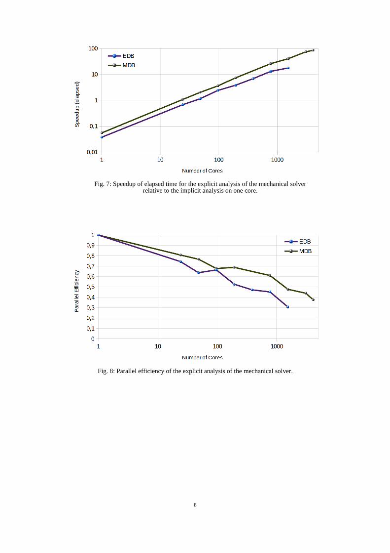
We also evaluated the scaling relative to the implicit analysis on only one core (Fig. 7). The base values decrease

according to the simulation time for the implicit analysis on one core, and the curves are shifted by constant

factors. The break-even point, namely the number of cores necessary to save time by using explicit analysis

instead of implicit analysis on one core, can be obtained from this graphic: For EDB it is 48 cores and for MDB

24 cores. The break-even point depends on the model size.

7

Fig. 5: Elapsed time for the explicit analysis (only the mechanical solver).

Fig. 6: Speedup of elapsed time for the explicit analysis (only the mechanical solver).

Regarding the parallel efficiency (the ratio of speedup and number of cores, Fig. 8), the larger model (MDB)

gains the better values: at 768 cores EDB has a ratio of 0.45, and MDB has a Ratio of 0.6. At the highest number

of cores (4080), this ratio decreases to 0.4 for MDB.

At last the ratio of elapsed time and CPU-time is of interest (Fig. 9). This ratio is nearly 1 with a small increase

above 3000 cores.

8

Fig. 7: Speedup of elapsed time for the explicit analysis of the mechanical solver relative to the implicit analysis on one core.

Fig. 8: Parallel efficiency of the explicit analysis of the mechanical solver.

9

Fig. 9: Ratio of elapsed time and CPU time for the explicit analysis (only the mechanical solver).

4. Implicit Analysis - Thermal Solution

The implicit analysis for the thermal solver is tested on all models.

The elapsed time over the number of cores is displayed in Fig. 10, the speedup of the elapsed time over the

number of cores is displayed in Fig. 11. All solid models provide a maximum speedup at 48 cores (2 nodes) in

the range from 5.3 to 6.7. The solid model without contact (RUP) and the metatransient model with contact

(SHT) have the best performance. The speedup increases nonlinearly, quasi asymptotically, up to its maximum

at 48 cores. Above 48 cores, the speedup decreases and the simulation time increases for the solid models.

The scaling behaviour of the shell element models (EDB, MDB) is linear up to the maximum tested number of

24 and 48 cores, respectively, with a speedup of 21 for MDB. Both models have identical speedup behaviour.

Fig. 10: Elapsed simulation time of the implicit analysis for the thermal solver.

10

Fig. 11: Elapsed speedup for implicit analysis thermal solver.

Considering the parallel efficiency (Fig. 12), the shell model MDB has a reasonable value of 0.45 at 48 cores,

but the values for the solid models lie in the range from 0.11 to 0.13 and are disappointing. The recommendation

for the thermal analysis of solid element models is to use jobs on 16 cores, because then the speedup is in the

range 4.1 to 5.5 and the parallel efficiency is in the range 0.25 to 0.34.

Fig. 12: Parallel efficiency of the implicit analysis of the thermal solver.

5. Implicit Analysis - Mechanical Solution

The implicit analysis for the mechanical solver is tested on all models except the large shell element model

(MDB).

The elapsed time over the number of cores is displayed in Fig. 13, the speedup of elapsed time over the number

of cores is displayed in Fig. 14. Two groups with different scaling behaviour can be identified: the models with

contact (RTS, MTS, SHT) and the models without contact (EDB, RUP). In the latter group the shell element

model (EDB) provides the same performance as the solid element model (RUP).

11

Unfortunately, in the current version the solid element model RTS does not run efficiently on more than 1 node

(24 cores). Neglecting the jobs with this defect, all solid element models with contact (MTS, SHT) show the

same scaling behaviour: The maximum speedup is reached at 48 cores with the range 5.1 to 5.6. Above 48 cores

the speedup decreases and the simulation time increases. The model size (RTS versus MTS) does not have a

significant influence on the scaling behaviour in the relevant range up to 24 cores.

The models without contact (EDB, RUP) provide a speedup at 96 cores in the range of 17.8 to 19.2. Jobs on

higher numbers of cores are not tested. Therefore, it cannot be assumed that the maximum of the speedup is

reached at 96 cores, the scaling may continue to increase.

Fig. 13: Elapsed simulation time for the implicit analysis of the mechanical solver.

Fig. 14: Elapsed speedup for the implicit analysis of the mechanical solver.

12

Fig. 15: Parallel efficiency for the implicit analysis of the mechanical solver.

Fig. 16: Ratio of elapsed time and CPU time for the implicit analysis of the mechanical solver.

Regarding the parallel efficiency (Fig. 15), reasonable values around 0.3 can be achieved for models with contact

with jobs on 16 cores and for models without contact with jobs on 48 cores. The speedup referring to this lies in

the range between 4.9 and 5.1 (for the models with contact on 16 cores) or in the range between 13.9 and 14.9

(for the models without contact on 48 cores).

The ratio of elapsed time and CPU time (Fig. 16) is increasing from quasi 1 up to 1.07 with increasing number of

cores. Highest ratio at 96 processes has the shell element model (EDB) followed by the solid element model

without contact (RUP).

6. Results and Recommendations

The scaling behaviour is mainly influenced by the model type and its numerical features (with or without

contact, shell or solid element model) and secondarily from the model size. Moreover, there is a strong

difference between explicit and implicit analysis. Which model type can be used, depends on the welding task.

As a consequence of this, a more detailed examination and discussion of the results and recommendations is

necessary.

13

A difference in the performance between transient and metatransient models was not recognised.

The advantage in performance for the explicit analysis is in opposition to its limitation to small time steps. Only

short processes with high welding speeds are suitable for the use of the explicit analysis.

To obtain best performance, the decoupled method is mandatory for some model types because the performance

differs between thermal and mechanical solvers. In a coupled analysis, the speedup limitation of one solver may

badly influence the performance of the other solver. This has been proved in the test case using the explicit

analysis on 4080 Cores for the mechanical solver. The performance, which could be achieved in this case, would

never be reached by a coupled thermal - mechanical analysis.

As a rule of thumb,

Shell element models show a better performance than solid element models,

Models without contact show a better performance than models with contact,

Large models show a better performance than small models.

Table 2 summarises the recommendations for the number of cores to be chosen for welding structure analyse

jobs for different model types.

Thermal analysis Mechanical analysis

Maximum

number of

cores

Speedup

at max number

of cores

Maximum

number of

cores

Speedup

at max number

of cores

Implicit

SHELL model without contact 48 (or higher) 21 48 14 - 15

SOLID model without contact 16 4 - 5 16 5

SOLID model with contact 16 4 - 5 16 5

Explicit

SHELL model without contact n.a n.a. 4080 (or higher) 1540

Table 2: Recommendation for the maximum number of cores for different welding structure analyse types.

7. High Performance Computing for SMEs

Small enterprises as engineering offices like ITL (Ingenieurbüro Tobias Loose) need to focus on modelling and

engineering type of work. There is too less time to get deep insight into scripting or programming know-how,

even for the usage of internal standard computer systems. Therefore, for these companies high performance

computing needs to be offered in an easy to use way.

As a result of this project, ITL can confirm that HLRS does a very good job by offering an easy to use

environment on the CRAY XC40 and by providing helpful support for its use. By making use of these service

offerings, HPC can become a well usable technology also for small enterprises with less experience in

specialized HPC computing platforms.

8. Conclusions

The performance on a supercomputer for parallelised jobs of different model types for welding structure analysis

of different welding tasks was examined. The welding tasks represent industrial cases.

As a result recommendations for the number of cores in order to obtain the optimal performance are provided

and the expected speedup is given. Both the number of the cores and the speedup depend on the model type.

14

During the SHAPE project, ITL got significant knowledge and experience in HPC. The project clarified how

HPC can be used for welding analysis consulting jobs. In more detail, which welding processes, welding tasks,

modelling methods and analysis types are applicable on HPC and how much effort is necessary.

The overall effort for welding analysis on HPC is now much better known with the help of this SHAPE project,

leading to the ability of a more accurate cost estimate of welding consulting jobs. This is a commercial benefit

for ITL.

This project provides a good basis for further investigations in high performance computing for welding

structure analysis. For example, the mass scaling or selective mass scaling [12] could help the explicit analysis to

overcome the time step limitation, but the result quality still needs to be tested for the special case of weld

analysis.

For future industrial consulting jobs, ITL will use the commercialised ways to access HLRS's supercomputing

facilities like e.g. CRAY XC40.

It is planned to publish the results of this SHAPE project at two conferences and in three technical journals:

14. LS-DYNA Forum, 10th

- 12th

October 1016 in Bamberg, Germany,

Simulationsforum für Wärmebehandlung und Schweißen, 8th

- 10th

November 2016, Weimar, Germany,

Journal „Schweiß- und Prüftechnik“,

Journal „Welding and Cutting“,

Journal „inSIDE - Innovatives Supercomputing in Germany“.

Acknowledgements

This work was financially supported by the PRACE project funded in part by the EU’s Horizon 2020 research

and innovation programme (2014-2020) under grant agreement 653838.

References

[1] Loose, T.: Schweißsimulation - Potentiale und Anwendungen. In: 26. Schweißtechnische Fachtagung 2016

Magdeburg, Verlag Otto-von-Guerike-Universität Magdeburg

[2] Brand, M.; Loose, T.: Anwendungsgebiete und Chancen der Schweißsimulation. In: Schweiß-und

Prüftechnik (2014) ÖGS Österreichische Gesellschaft für Schweißtechnik (Hrsg.), Nr.05-06, pp 138-142,

Wien

[3] Loose, T.; Boese, B.: Leistungsfähigkeit der Schweißstruktursimulation im Schienenfahrzeugbau. In:

Vortragsband 10. Fachtagung Fügen und Konstruieren im Schienenfahrzeugbau, 2013, pp 61 - 67, Halle

[4] Loose, T.: Einfluß des transienten Schweißvorganges auf Verzug, Eigenspannungen und Stabiltiätsverhalten

axial gedrückter Kreiszylinderschalen aus Stahl, Diss, 2007

[5] http://www.tl-ing.de/produkte/dynaweld/

[6] Loose, T.; Mokrov, O.: SimWeld and DynaWeld Software tools to setup simulation models for the analysis

of welded structures with LS-DYNA. In: 10th European LS-DYNA Conference 2015, Würzburg 15. - 17. 6.

2015

[7] Loose, T.; Mokrov, O.: SimWeld and DynaWeld - Software tools to setup simulation models for the

analysis of welded structures with LS-DYNA. In: Welding and Cutting 15 (2016) No. 3 pp 168 - 172

[8] Loose, T.: Einbindung der Schweißsimlation in die Fertigungssimulation mit SimWeld und DynaWeld. In:

DVS Congress 2015, DVS-Berichte Band 315, pp 860 - 865

[9] https://wickie.hlrs.de/platforms/index.php/Cray_XC40

[10] Bergman, G.; Oldenburg, M.: “A finite element model for thermomechanical analysis of sheet metal

forming”, Int. J. Numer. Meth. Engng. 59, pp. 1167–1186.

[11] LS-DYNA Theory Manual, 2006.

[12] Borrvall, Th.: “Selective Mass Scaling (SMS)”, LS-DYNA Information, DYNAmore GmbH, 2011.