
Shape optimization of 2D structures using simulated annealingweb.boun.edu.tr/sonmezfa/SHAPE...
21
Shape optimization of 2D structures using simulated annealing Fazil O. Sonmez * Department of Mechanical Engineering, Bogazici University, Istanbul, Bebek 34342, Turkey Received 13 September 2005; received in revised form 22 May 2006; accepted 11 January 2007 Available online 31 March 2007 Abstract The goal of this study is to obtain globally optimum shapes for two-dimensional structures subject to quasi-static loads and restraints. For this purpose a technique is proposed, using which the volume (or weight) of a structure can be minimized. The emphasis is on how one can define the shape precisely, and find a shape that accurately reflects the globally optimum shape. As design constraints, stresses developed in the structure should not exceed the maximum allowable stress, and connectivity of the structure should not be lost during shape changes. Optimization is achieved by a stochastic search algorithm called direct simulated annealing (DSA), which seeks the global minimum through randomly generated configurations. In order to obtain random configura- tions, a boundary variation technique is used. In this technique, a set of key points is chosen and connected by cubic splines to describe the boundary of the structure. Whenever the positions of the key points are changed in random directions, a new shape is obtained. Thus, coordinates of the key points serve as design variables. In order to apply the optimization procedure, a general computer code was devel- oped using ANSYS Parametric Design Language. A number of cases were examined to test its effectiveness. The results show that this technique can be applied to two-dimensional shape optimization problems with high reliability even for cases where the entire free boundary is allowed to vary. Ó 2007 Elsevier B.V. All rights reserved. Keywords: Direct search simulated annealing (DSA); Boundary variation; Precision; Accuracy; FEM; 2D structures 1. Introduction The increasing demand for lightweight, high-perfor- mance, low-cost structures, drives the considerable current research going on in the field of structural optimization. Studies on shape optimization [1–87] attest that shape changes may lead to considerable savings in weight and improvements in structural performance. Applications in this field include optimum shape designs of fillets [4,7,9, 12,20,25,27,30,43,50,51,53,66,71,80,85,87], cams [61], holes in plates [3,7,9,10,12,19,22,25–28,32,39,41,42,60,66,73,76, 80,83,85,87] for single and multiple [68] load cases, rings [30], torque arms [6,20,27,38,62,71,84], connecting rods [31,53,74,79,83], brackets [6,38,62,79,84], chain links [10,27,77], hooks [20,42], torque converter subject to pres- sure and centrifugal loads [69], uniaxially loaded plate with a hole [77], bridge under moving [76] and static [73] loads, plates containing cracks [37], plates with a notch [35,59,85], 2D structures subject to fatigue loading [74], 2D structures subject to thermomechanical boundary conditions [57], 2D structures containing a crack [55], various other 2D struc- tures [39,48,65,70], saw blades [23], cantilever beams [21,24,28,29,35,41,53,60,64,70,88], beams subject to tor- sional loading [49], beams with thin-walled sections [44], axially excited beams [72], thin-walled tubes subject to tor- sional loading [77], shells under dynamic loading [67], com- ponents which are in contact [40,46,54,56,75,83], wheel profile of railway vehicles [81], thermal fins [17,58], axisym- metric structures [78], 3D structures like engine bearing cap [11], cantilevered thick plate with a hole though the thick- ness [16,47], aircraft turbine disk [16], control arm [63], engine mount bracket [63], and slider bearings [82]. The general purpose of shape optimization is to find the best profile for a structure under various constraints 0045-7825/$ - see front matter Ó 2007 Elsevier B.V. All rights reserved. doi:10.1016/j.cma.2007.01.019 * Tel.: +90 212 359 7196; fax: +90 212 287 2456. E-mail address: [email protected] www.elsevier.com/locate/cma Comput. Methods Appl. Mech. Engrg. 196 (2007) 3279–3299
-
Upload
phungnguyet -
Category
Documents
-
view
231 -
download
0
Transcript of Shape optimization of 2D structures using simulated annealingweb.boun.edu.tr/sonmezfa/SHAPE...
www.elsevier.com/locate/cma
Comput. Methods Appl. Mech. Engrg. 196 (2007) 3279–3299
Shape optimization of 2D structures using simulated annealing
Fazil O. Sonmez *
Department of Mechanical Engineering, Bogazici University, Istanbul, Bebek 34342, Turkey
Received 13 September 2005; received in revised form 22 May 2006; accepted 11 January 2007Available online 31 March 2007
Abstract
The goal of this study is to obtain globally optimum shapes for two-dimensional structures subject to quasi-static loads and restraints.For this purpose a technique is proposed, using which the volume (or weight) of a structure can be minimized. The emphasis is on howone can define the shape precisely, and find a shape that accurately reflects the globally optimum shape.
As design constraints, stresses developed in the structure should not exceed the maximum allowable stress, and connectivity of thestructure should not be lost during shape changes. Optimization is achieved by a stochastic search algorithm called direct simulatedannealing (DSA), which seeks the global minimum through randomly generated configurations. In order to obtain random configura-tions, a boundary variation technique is used. In this technique, a set of key points is chosen and connected by cubic splines to describethe boundary of the structure. Whenever the positions of the key points are changed in random directions, a new shape is obtained. Thus,coordinates of the key points serve as design variables. In order to apply the optimization procedure, a general computer code was devel-oped using ANSYS Parametric Design Language. A number of cases were examined to test its effectiveness. The results show that thistechnique can be applied to two-dimensional shape optimization problems with high reliability even for cases where the entire freeboundary is allowed to vary.� 2007 Elsevier B.V. All rights reserved.
Keywords: Direct search simulated annealing (DSA); Boundary variation; Precision; Accuracy; FEM; 2D structures
1. Introduction
The increasing demand for lightweight, high-perfor-mance, low-cost structures, drives the considerable currentresearch going on in the field of structural optimization.Studies on shape optimization [1–87] attest that shapechanges may lead to considerable savings in weight andimprovements in structural performance. Applications inthis field include optimum shape designs of fillets [4,7,9,12,20,25,27,30,43,50,51,53,66,71,80,85,87], cams [61], holesin plates [3,7,9,10,12,19,22,25–28,32,39,41,42,60,66,73,76,80,83,85,87] for single and multiple [68] load cases, rings[30], torque arms [6,20,27,38,62,71,84], connecting rods[31,53,74,79,83], brackets [6,38,62,79,84], chain links[10,27,77], hooks [20,42], torque converter subject to pres-
0045-7825/$ - see front matter � 2007 Elsevier B.V. All rights reserved.
doi:10.1016/j.cma.2007.01.019
* Tel.: +90 212 359 7196; fax: +90 212 287 2456.E-mail address: [email protected]
sure and centrifugal loads [69], uniaxially loaded plate witha hole [77], bridge under moving [76] and static [73] loads,plates containing cracks [37], plates with a notch [35,59,85],2D structures subject to fatigue loading [74], 2D structuressubject to thermomechanical boundary conditions [57], 2Dstructures containing a crack [55], various other 2D struc-tures [39,48,65,70], saw blades [23], cantilever beams[21,24,28,29,35,41,53,60,64,70,88], beams subject to tor-sional loading [49], beams with thin-walled sections [44],axially excited beams [72], thin-walled tubes subject to tor-sional loading [77], shells under dynamic loading [67], com-ponents which are in contact [40,46,54,56,75,83], wheelprofile of railway vehicles [81], thermal fins [17,58], axisym-metric structures [78], 3D structures like engine bearing cap[11], cantilevered thick plate with a hole though the thick-ness [16,47], aircraft turbine disk [16], control arm [63],engine mount bracket [63], and slider bearings [82].
The general purpose of shape optimization is to find thebest profile for a structure under various constraints
3280 F.O. Sonmez / Comput. Methods Appl. Mech. Engrg. 196 (2007) 3279–3299
imposed by the requirements of the design. The optimumshape provides either the most efficient and effective useof material or the best performance. Accordingly, in someof the studies the goal was to minimize weight of the struc-ture [10,11,16,17,20,24,25,30,31,35,38–41,48,49,51,53,62,69–71,77–79,84], in others to increase mechanical perfor-mance, e.g. to minimize stress concentration [3,19,22,25,26,32,33,42,43,57,60,66,68,77,83,87], maximize fracturestrength [37,80,85], buckling strength [65], fatigue life[50,55,59,68], and heat flux [17,58], minimize peak contactstress [46,54,56,75,83], compliance [7,29,34,48,63,64,67,70,57,73,78], peak acceleration [67], and the probabilityof failure for brittle materials [23], and optimize dynamicbehavior of structures [44,52,72,88].
In order to optimize a structure, some of its propertiesaffecting the cost function should be changed. As for ashape optimization problem, the boundary should beallowed to vary. In previous studies, boundaries of thestructures were usually defined by spline curves [9,11,23–25,28,31,35,39–41,46,47,51,56–61,65,66,69–71,76,77,87,88]passing through a number of key points. Positions of thesepoints thus become design variables. NURBS curves [27]defined by a polygon can also be used to define a shape.Weights at each vertex of the polygon then become designvariables. Some parameterized equations can be used forboundary curve [26,30,34]; the parameters then controlthe size, shape and aspect ratio of the boundary. Theadvantage of using these curves is that one may definethe shape of the model using just a few design variablesand obtain a smooth boundary. Alternatively, in a numberof studies [3,32,43,64,68,83] all or some of the nodes at theboundaries were allowed to change their positions; or mag-nitudes of a set of fictitious loads on the boundary nodeswere changed [10]; or more simply dimensions of individualparts of the structures were taken as design variables[29,52]. Also, by removing or restoring materials withinthe elements of the finite element model, the shape of thestructure may be changed [20,26,49,74,75,80]. In that case,presence of material becomes a design variable.
During a shape optimization process, geometry of thestructure may undergo substantial changes, such that itcan no longer be considered as a viable structure, e.g. geo-metric model may become unfeasible [20,21], stresses mayexceed the admissible stress level [20,21,24,29–31,35,38–41,51,62,71,78,79,84], fatigue life may be shorter than thelowest allowable number of cycles [74], natural frequencymay be lower than a certain limit [24], displacements maybe too large [11,16,24,35], finite element mesh may becometoo distorted [59], the area or volume may become toolarge [7,29,46,65,67,72,73,88], manufacturing may becometoo difficult [59]. In these cases, behavioral or side con-straints should be imposed.
Locating globally optimum shape designs is a difficultproblem, requiring sophisticated optimization procedures.In typical structural optimization problems, there may bemany locally minimum configurations. For that reason, adownhill-proceeding algorithm, in which a monotonically
decreasing value of objective function is iteratively created,may get stuck into a locally minimum point other than theglobally minimum solution. Its success depends on thechoice of initial design. The usual approach is to employthe algorithm many times starting from different configura-tions with the hope that one of the initial positions be suf-ficiently close to the globally minimum configuration, andthen to choose the lowest value as the globally minimumsolution. Another disadvantage is that if the starting pointis outside the feasible region, the algorithm may convergeto a local minimum within the infeasible domain.
If a downhill-proceeding local search algorithm is used,an optimization procedure can only be successful if it isused to improve the current design [4,69,83] or only a smallsegment of the boundary is allowed to move [3,4,9,12,19,26,28,35,39,43,53,69], or only a small number of dimen-sional parameters are used to define its shape [6,26,29,30].The advantage of using these algorithms, on the otherhand, is their computational efficiency. Just a small numberof iterations are needed to obtain an improved design.
One of the optimization methods that have been used toobtain optimum structural designs is evolutionary struc-tural optimization. The approach is to gradually removeinefficient materials until the shape of the structure evolvesinto an optimum. Although this method is not a globalsearch algorithm, because of its simplicity and effectiveness,it has been applied to many structural optimization prob-lems [49,74–76,80]. This method is also suitable for topol-ogy optimization, where not only outer boundary butalso geometry of inner regions is allowed to change. Thereare also similar algorithms which can effectively be used tofind improved designs such as biological growth methods[19,38,66] and metamorphic development methods [78].
In order to find the absolute minimum of an objectivefunction without being sensitive to the starting position, aglobal optimization method has to be employed in struc-tural optimization problems. Stochastic optimization tech-niques are quite suitable in this respect. Among theiradvantages, they are not sensitive to starting point, theycan search a large solution space, and they can escape localoptimum points because they allow occasional uphillmoves. The genetic algorithm (GA) and simulated anneal-ing (SA) algorithm are two of the most popular stochasticoptimization techniques.
Genetic algorithms found many applications on shapeoptimization problems [15,21,31,41,47,48,61,64,70,57,77,79]. They are based on the concepts of genetics and Dar-winian survival of the fittest [13]. The idea is to start thesearch process with a set of designs, called population.The search procedure is a simulation of the evolution pro-cess. The genetic algorithm transforms one population intoa succeeding population using operators of reproduction,recombination, and mutation. The convergence to the glo-bal minimum depends on the proper choice of the designparameters, rules of the reproduction and mutation.
Kirkpatrick et al. [89] first proposed simulated annealing(SA) as a powerful stochastic search technique. The main
F1
P1
F3
F2
x
y
Fig. 1. Representation of a 2D shape optimization problem.
F.O. Sonmez / Comput. Methods Appl. Mech. Engrg. 196 (2007) 3279–3299 3281
advantage of SA is that it is generally more reliable in findingthe global optimum, i.e. the probability of locating theglobal optimum is high even with large numbers of designvariables. Application of simulated annealing to shape opti-mization of the structures is quite rare. Anagnostou and hiscoworkers [17] used SA to design a thermal fin with mini-mum material use. Shim and Manoochehri [20] used SA toobtain optimal designs for two-dimensional structures witha minimum use of material. In their approach, a structurewas first divided into a number of small finite element blocksand then these blocks were randomly removed or restored toobtain a randomly generated new shape. One difficulty withthis method is that removing and restoring an element mayviolate model connectivity. Whenever a new configuration isgenerated its connectivity should be checked by a compli-cated algorithm. Another difficulty is the roughness of theresulting boundaries. If smooth boundaries are desired,small elements should be used, resulting in long computa-tional times. However, their study demonstrated the prom-ise of SA in solving shape optimization problems.
The ultimate goal of a designer in using a shape optimiza-tion algorithm is just to state the boundary conditions and letthe algorithm do some iterations without human interven-tion and automatically produce the best design. In thisrespect, the previous studies had only a relative success.Many of them relied too much on designer’s intuition, orimposed tight restrictions on the movements of boundary,or fixed some portions of boundary so that the number ofpossible designs among which the algorithm may searchthe optimum one was quite limited. This study attempts tocome one step closer to our ultimate goal. The proceduredeveloped in this study may start from almost any initialmodel thanks to the global search algorithm used. In factthe only interactive effort required from the designer is toprovide an initial coarse boundary model consisting of splinecurves passing through the given key points, and to specifythe boundary conditions and which key points of the bound-ary are allowed to move during the optimization process.
Another requirement for the search of globally optimumconfiguration is the precise definition of the optimized sys-tem. If the system is complex, complete definition of it mayrequire large numbers of design variables. If all of them areused as optimization variables, that means if the optimizedsystem is precisely defined, long computational times areneeded, and also likelihood of locating the optimum designmay become very low. If the definition of the system isbased on a limited number of design variables, that meansif the definition allows for only a limited number of distinctconfigurations, the resulting optimum configuration maynot reflect the best possible design. Although using themost precise definition of the system during optimizationis desirable, this is usually not practicable; but if a less pre-cise definition is used, one should be aware of its impact onhow well the final design represents the best possibledesign. To the author’s knowledge, there is no study onstructural optimization, or specifically on shape optimiza-tion in which precision was a main concern. Apparently,
in most of the previous studies, definition of shape wasnot precise enough to be capable of representing the bestpossible shape. In this study, on the other hand, a proce-dure is proposed to monitor precision so that a reasonablecompromise can be made between a better definition and ashorter computational time.
Another concern in shape optimization is the accuracy,i.e. how well the resulting optimum shape reflects the bestpossible shape. In many of the previous studies, the goalwas to improve an intuitively found current design througha local search algorithm rather than to find the best possibleshape. In some of them, global search algorithms were used,but the accuracy remained questionable. In this study, anumber of methods are proposed to achieve high accuracy.
2. Problem statement
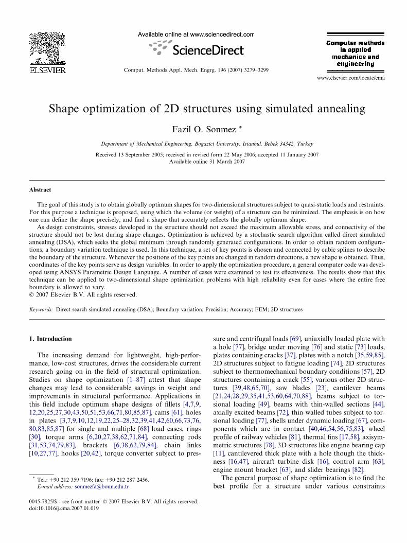
Consider a two-dimensional structure as in Fig. 1 havinga geometry that can be defined by its boundary and thick-ness. The structure is subject to in-plane quasi-static loads;it is also restrained from moving at some points of theboundary. Applied loads and restraints are considered asboundary conditions. The structure should be able to resistthe loads without failure. This means the material shouldnot yield. Besides, no part of the structure is to lose its con-nection to the restraints; i.e. the structure should remain inone piece. These are the two constraints imposed on thestructure. Our objective is to minimize the volume (orweight) of the structure, in other words, to obtain a config-uration (shape) with the most efficient use of material with-out violating the behavioral and geometric constraints.
The shape optimization problem for minimum weightcan be formulated briefly as
Given:
initial positions of key points, boundaryconditions (applied forces and restraints),material propertiesFind:
the optimum shape of the structure Minimize: V = volume of the structure Subject to: (i) the stress constraint (rmax 6 rallow)(ii) the geometric constraint (modelconnectivity)
Designvariables:
the positions of the key points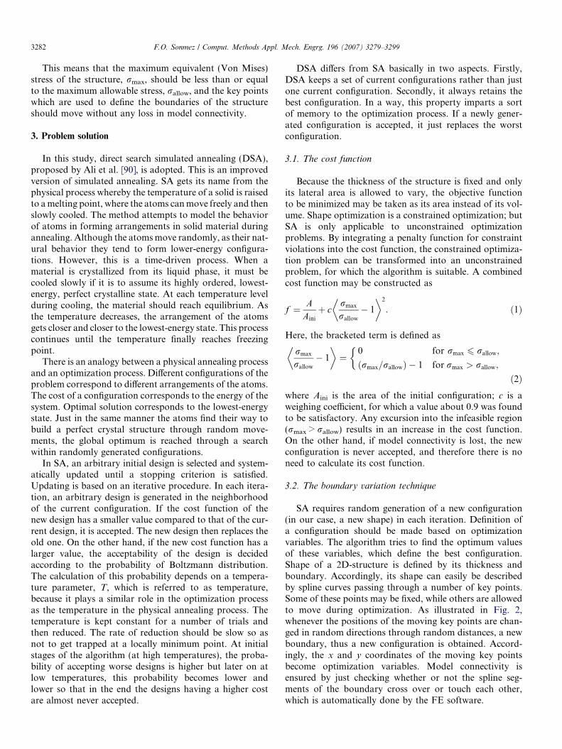
3282 F.O. Sonmez / Comput. Methods Appl. Mech. Engrg. 196 (2007) 3279–3299
This means that the maximum equivalent (Von Mises)stress of the structure, rmax, should be less than or equalto the maximum allowable stress, rallow, and the key points
which are used to define the boundaries of the structureshould move without any loss in model connectivity.3. Problem solution
In this study, direct search simulated annealing (DSA),proposed by Ali et al. [90], is adopted. This is an improvedversion of simulated annealing. SA gets its name from thephysical process whereby the temperature of a solid is raisedto a melting point, where the atoms can move freely and thenslowly cooled. The method attempts to model the behaviorof atoms in forming arrangements in solid material duringannealing. Although the atoms move randomly, as their nat-ural behavior they tend to form lower-energy configura-tions. However, this is a time-driven process. When amaterial is crystallized from its liquid phase, it must becooled slowly if it is to assume its highly ordered, lowest-energy, perfect crystalline state. At each temperature levelduring cooling, the material should reach equilibrium. Asthe temperature decreases, the arrangement of the atomsgets closer and closer to the lowest-energy state. This processcontinues until the temperature finally reaches freezingpoint.
There is an analogy between a physical annealing processand an optimization process. Different configurations of theproblem correspond to different arrangements of the atoms.The cost of a configuration corresponds to the energy of thesystem. Optimal solution corresponds to the lowest-energystate. Just in the same manner the atoms find their way tobuild a perfect crystal structure through random move-ments, the global optimum is reached through a searchwithin randomly generated configurations.
In SA, an arbitrary initial design is selected and system-atically updated until a stopping criterion is satisfied.Updating is based on an iterative procedure. In each itera-tion, an arbitrary design is generated in the neighborhoodof the current configuration. If the cost function of thenew design has a smaller value compared to that of the cur-rent design, it is accepted. The new design then replaces theold one. On the other hand, if the new cost function has alarger value, the acceptability of the design is decidedaccording to the probability of Boltzmann distribution.The calculation of this probability depends on a tempera-ture parameter, T, which is referred to as temperature,because it plays a similar role in the optimization processas the temperature in the physical annealing process. Thetemperature is kept constant for a number of trials andthen reduced. The rate of reduction should be slow so asnot to get trapped at a locally minimum point. At initialstages of the algorithm (at high temperatures), the proba-bility of accepting worse designs is higher but later on atlow temperatures, this probability becomes lower andlower so that in the end the designs having a higher costare almost never accepted.
DSA differs from SA basically in two aspects. Firstly,DSA keeps a set of current configurations rather than justone current configuration. Secondly, it always retains thebest configuration. In a way, this property imparts a sortof memory to the optimization process. If a newly gener-ated configuration is accepted, it just replaces the worstconfiguration.
3.1. The cost function
Because the thickness of the structure is fixed and onlyits lateral area is allowed to vary, the objective functionto be minimized may be taken as its area instead of its vol-ume. Shape optimization is a constrained optimization; butSA is only applicable to unconstrained optimizationproblems. By integrating a penalty function for constraintviolations into the cost function, the constrained optimiza-tion problem can be transformed into an unconstrainedproblem, for which the algorithm is suitable. A combinedcost function may be constructed as
f ¼ AAini
þ crmax
rallow
� 1
� �2
: ð1Þ
Here, the bracketed term is defined as
rmax
rallow
� 1
� �¼
0 for rmax 6 rallow;
ðrmax=rallowÞ � 1 for rmax > rallow;
�
ð2Þwhere Aini is the area of the initial configuration; c is aweighing coefficient, for which a value about 0.9 was foundto be satisfactory. Any excursion into the infeasible region(rmax > rallow) results in an increase in the cost function.On the other hand, if model connectivity is lost, the newconfiguration is never accepted, and therefore there is noneed to calculate its cost function.
3.2. The boundary variation technique
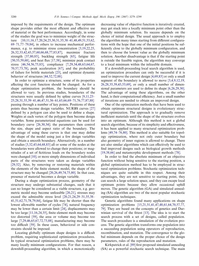
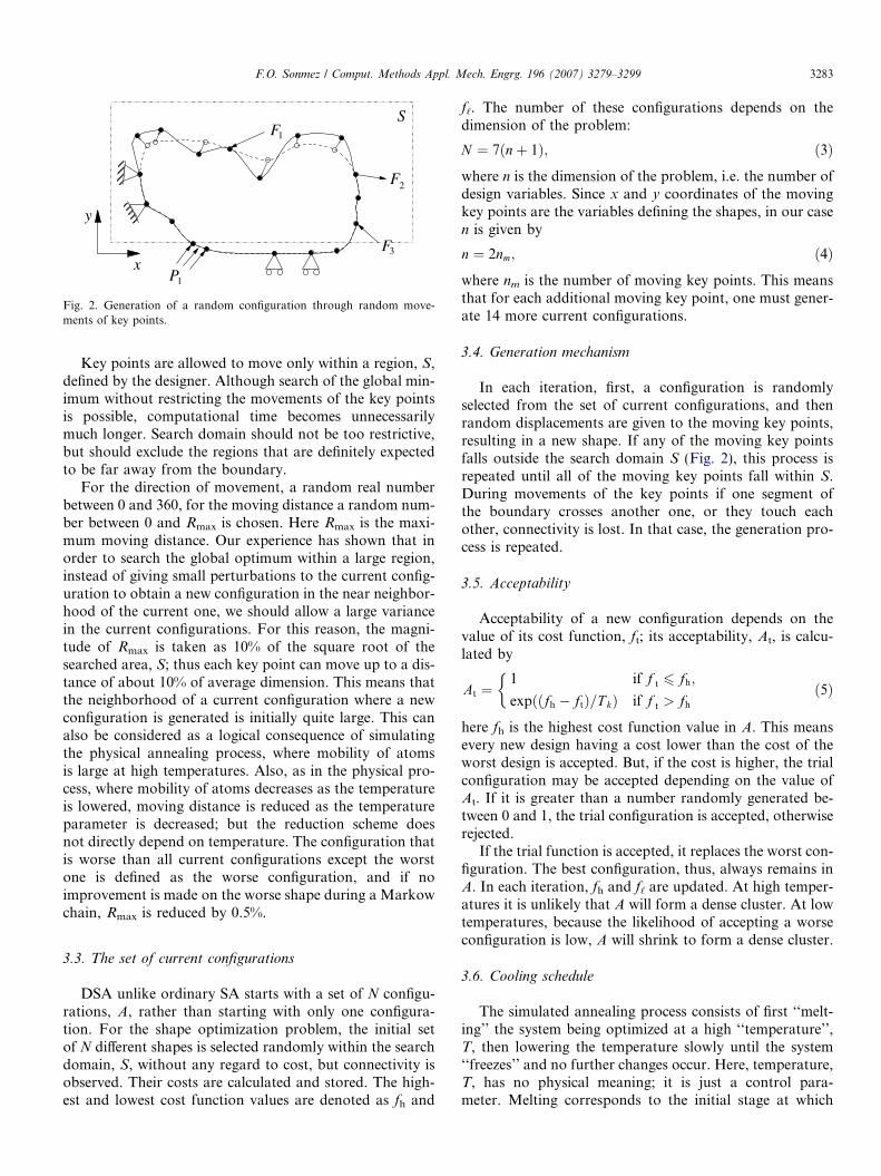
SA requires random generation of a new configuration(in our case, a new shape) in each iteration. Definition ofa configuration should be made based on optimizationvariables. The algorithm tries to find the optimum valuesof these variables, which define the best configuration.Shape of a 2D-structure is defined by its thickness andboundary. Accordingly, its shape can easily be describedby spline curves passing through a number of key points.Some of these points may be fixed, while others are allowedto move during optimization. As illustrated in Fig. 2,whenever the positions of the moving key points are chan-ged in random directions through random distances, a newboundary, thus a new configuration is obtained. Accord-ingly, the x and y coordinates of the moving key pointsbecome optimization variables. Model connectivity isensured by just checking whether or not the spline seg-ments of the boundary cross over or touch each other,which is automatically done by the FE software.
F1
P1
F3
F2
x
y
S
Fig. 2. Generation of a random configuration through random move-ments of key points.
F.O. Sonmez / Comput. Methods Appl. Mech. Engrg. 196 (2007) 3279–3299 3283
Key points are allowed to move only within a region, S,defined by the designer. Although search of the global min-imum without restricting the movements of the key pointsis possible, computational time becomes unnecessarilymuch longer. Search domain should not be too restrictive,but should exclude the regions that are definitely expectedto be far away from the boundary.
For the direction of movement, a random real numberbetween 0 and 360, for the moving distance a random num-ber between 0 and Rmax is chosen. Here Rmax is the maxi-mum moving distance. Our experience has shown that inorder to search the global optimum within a large region,instead of giving small perturbations to the current config-uration to obtain a new configuration in the near neighbor-hood of the current one, we should allow a large variancein the current configurations. For this reason, the magni-tude of Rmax is taken as 10% of the square root of thesearched area, S; thus each key point can move up to a dis-tance of about 10% of average dimension. This means thatthe neighborhood of a current configuration where a newconfiguration is generated is initially quite large. This canalso be considered as a logical consequence of simulatingthe physical annealing process, where mobility of atomsis large at high temperatures. Also, as in the physical pro-cess, where mobility of atoms decreases as the temperatureis lowered, moving distance is reduced as the temperatureparameter is decreased; but the reduction scheme doesnot directly depend on temperature. The configuration thatis worse than all current configurations except the worstone is defined as the worse configuration, and if noimprovement is made on the worse shape during a Markowchain, Rmax is reduced by 0.5%.
3.3. The set of current configurations
DSA unlike ordinary SA starts with a set of N configu-rations, A, rather than starting with only one configura-tion. For the shape optimization problem, the initial setof N different shapes is selected randomly within the searchdomain, S, without any regard to cost, but connectivity isobserved. Their costs are calculated and stored. The high-est and lowest cost function values are denoted as fh and
f‘. The number of these configurations depends on thedimension of the problem:
N ¼ 7ðnþ 1Þ; ð3Þwhere n is the dimension of the problem, i.e. the number ofdesign variables. Since x and y coordinates of the movingkey points are the variables defining the shapes, in our casen is given by
n ¼ 2nm; ð4Þwhere nm is the number of moving key points. This meansthat for each additional moving key point, one must gener-ate 14 more current configurations.
3.4. Generation mechanism
In each iteration, first, a configuration is randomlyselected from the set of current configurations, and thenrandom displacements are given to the moving key points,resulting in a new shape. If any of the moving key pointsfalls outside the search domain S (Fig. 2), this process isrepeated until all of the moving key points fall within S.During movements of the key points if one segment ofthe boundary crosses another one, or they touch eachother, connectivity is lost. In that case, the generation pro-cess is repeated.
3.5. Acceptability
Acceptability of a new configuration depends on thevalue of its cost function, ft; its acceptability, At, is calcu-lated by
At ¼1 if f t 6 fh;
expððfh � ftÞ=T kÞ if f t > fh
�ð5Þ
here fh is the highest cost function value in A. This meansevery new design having a cost lower than the cost of theworst design is accepted. But, if the cost is higher, the trialconfiguration may be accepted depending on the value ofAt. If it is greater than a number randomly generated be-tween 0 and 1, the trial configuration is accepted, otherwiserejected.
If the trial function is accepted, it replaces the worst con-figuration. The best configuration, thus, always remains inA. In each iteration, fh and f‘ are updated. At high temper-atures it is unlikely that A will form a dense cluster. At lowtemperatures, because the likelihood of accepting a worseconfiguration is low, A will shrink to form a dense cluster.
3.6. Cooling schedule
The simulated annealing process consists of first ‘‘melt-ing’’ the system being optimized at a high ‘‘temperature’’,T, then lowering the temperature slowly until the system‘‘freezes’’ and no further changes occur. Here, temperature,T, has no physical meaning; it is just a control para-meter. Melting corresponds to the initial stage at which
3284 F.O. Sonmez / Comput. Methods Appl. Mech. Engrg. 196 (2007) 3279–3299
configurations are generated within the solution domain, S,without much regard to the cost. At high temperatures,(high values of T) the probability of acceptance is high asEq. (5) implies. Accordingly, configurations that have evenvery high cost values may be accepted, just as in the phys-ical annealing process the atoms in the melting state mayform configurations having very high energy. At low valuesof temperature parameter, acceptability becomes low andacceptance of worse configurations is then unlikely, justas the atoms become stable, and do not tend to changetheir arrangements at low temperatures. The cooling sche-dule in SA controls the convergence of the algorithm to theglobal minimum just as the cooling scheme in the physicalannealing process controls the final microstructure. There-fore, performance of SA depends on the cooling schedule.
In a cooling schedule, first an initial value, T0, should bespecified for the temperature parameter. A scheme is thenrequired for reducing T and for deciding how many trialsare to be attempted at each value of T. Lastly, the freezing(or final value of the) temperature parameter is specified.
Initial value of the temperature parameter: Its initialvalue should be high enough to allow nearly all trials tobe accepted. This provides complete ‘‘melting’’ at the initialstages of the optimization process. Otherwise, the regionwill not be thoroughly searched and thus the algorithmmay become trapped in a local minimum. In the physicalanalogy mentioned earlier, choosing high T0 correspondsto heating up the solid until all particles are randomlyarranged in the liquid phase such that atoms may freelyarrange themselves.
Length of the Markow chains: Iterations during whichthe value of the temperature parameter, T, is kept constantare called Markov chains (or inner loops). Ali et al. [90]adopted the following equation to decide on the length ofa Markow chain (the number of trials (or iterations)) forthe kth level of T:
Lk ¼ Lþ Lð1� ef‘�fhÞ: ð6Þ
Here
L ¼ 10n; ð7Þ
where n is the dimension of the problem given by Eq. (4).At high temperatures, the current configurations form asparse cluster; consequently fh � f‘ is large and Markowchain length is close to 2L. On the other hand, when theyform a dense cluster at low temperatures, it approachesto L. During the execution of kth Markow chain withlength Lk, if a configuration is generated having a cost lessthan f‘, the best value in A, the current chain is stopped,and a new Markow chain is started. If a configuration bet-ter than the best configuration in A is not found, the com-plete chain of length Lk is executed.
The scheme for decreasing the temperature parameter:After the initial value of the temperature parameter, T0,is determined, a decrement rule must be established to findthe subsequent values of the temperature parameter. Theprobability of reaching the global optimum solution
depends on how fast the value of the temperature parame-ter is lowered. If the cooling rate is fast, the optimizationprocess will probably end up with one of the higher-costlocal minima. If the cooling rate is slow, the reliability offinding the global optimum solution will be high, but, theoptimization process will take excessively long time. There-fore, the choice of the cooling schedule determines theeffectiveness of the algorithm.
In DSA, a temperature scale factor, (ak+1), is specified tocalculate the value of the temperature parameter in the nextMarkow chain, Tk+1.
T kþ1 ¼ akþ1T k; ð8Þ
where Tk is the value of the current temperature. A valuefor akþ1 2 ½amin; amax� is calculated using the following equa-tion [90]:
akþ1 ¼amax if Lk > L0k;
ak � ðak � aminÞð1� L0k�1=LkÞ else if Lk > L0k�1;
amax � ðamax � akÞðLk=L0k�1Þ else Lk 6 L0k�1;
8><>:
ð9Þ
where L0k is the actual number of trials executed in the kthMarkow chain. If no configuration is found in the kth Mar-kow chain (inner loop) that is better than the best currentconfiguration L0k is set to the value of Lk. If a configurationwhich is better than all is found, the inner loop is termi-nated, and L0k is set to the number of iterations actually exe-cuted in this loop. In this study, amax = 0.999 andamin = 0.99 were chosen as appropriate values, which pro-vided a compromise between the two effectiveness criteria,i.e. short computational time and high reliability of locat-ing global minimum. Initial value of a is taken as the aver-age of amax and amin.
Because, a new configuration is generated by giving per-turbations to a configuration selected randomly among alarge number of current configurations, and once acceptedthe new configuration replaces only the worst one, coolingrate has less importance in DSA in comparison to conven-tional SA. The worst configuration seldom plays a role inthe generation process. Again, it is important to start witha temperature high enough to accept almost all generatedconfigurations.
Stopping criterion: The optimization process is termi-nated when no further appreciable improvement can beachieved. This occurs when three conditions are satisfied.Firstly, the current temperature parameter should be small,in other words it should be close to the ‘‘freezing tempera-ture’’ (zero), i.e. no further worse designs may be accepted.Secondly, the current configurations, A, should form adense cluster; thus all alternatives were eliminated and opti-mization process converged to a single configuration.Thirdly, the maximum moving distance of key points,Rmax, should be small; this means the neighborhood ofthe current configurations within which optimum designis sought became very small. Accordingly, the stopping cri-terion can be expressed as
F.O. Sonmez / Comput. Methods Appl. Mech. Engrg. 196 (2007) 3279–3299 3285
fh � f‘ < e1 and
T k < e2 and
Rmax < e3;
ð10Þ
where ei are small numbers. For the optimization problemsthat were considered, it was more than sufficient to takee1 = e2 = 0.0001, and e3 = 0.05 mm for a good estimate
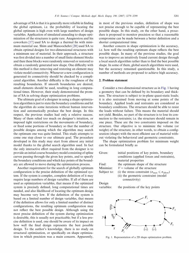
Fig. 3. The soluti
of the global minimum. The value of e3 depends on thedimensions of the structure.
3.7. Solution procedure
As a first step in the optimization procedure, thedesigner defines the force and displacement boundary
on procedure.
3286 F.O. Sonmez / Comput. Methods Appl. Mech. Engrg. 196 (2007) 3279–3299
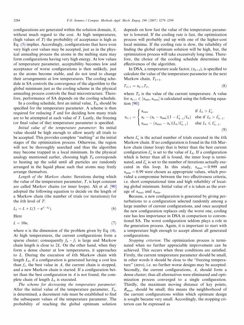
conditions, chooses the material, and decides on the num-ber of key points, the moving boundaries and how they areconnected. Fig. 3 describes the procedure followed in thisstudy to solve the optimization problem. First, N numberof initial configurations are randomly generated withinthe search domain, S; their costs are calculated and thebest, worse, and worst ones are determined. An initialvalue for the temperature parameter is chosen, whichshould be high enough to accept nearly all randomly gen-erated new shapes. In the figure, k and j show the innerloop (Markow chain) number and the number of generatedconfigurations in the current inner loop, respectively. Ineach iteration of the Markow chain, a new configurationis generated within the search domain, S, by giving randomdisplacements to the key points of a randomly chosen cur-rent configuration. If a key point falls outside S, randomrepositioning of this key point is repeated. If connectivityis lost, the generation process is repeated until a validgeometry is obtained. If the acceptability of the new config-uration calculated by Eq. (5) is greater than a randomlygenerated number, it is accepted, replacing the worst con-figuration. If its cost is lower than the best cost, the innerloop is terminated; otherwise the iterations are continueduntil the iteration number, j, becomes equal to Lk calcu-lated by Eq. (6). When an inner loop ends, the temperatureparameter is decreased. With a lower temperature, accept-ability decreases as Eq. (5) implies. This means that a con-figuration having a cost higher than the cost of the worstconfiguration is less frequently accepted.
As in the physical annealing process where the mobilityof the atoms diminishes during cool down, mobility of thekey points is decreased as acceptability decreases. This isdone when a configuration is not found during a Markowloop which is better than the worse current configuration.In this way, the neighborhood of the current configurationswithin which a new configuration is generated narrowsdown as acceptability becomes lower and lower. If a shapehaving a cost lower than the cost of the worse current con-figuration is not found during the inner loop iterations, themaximum moving distance, Rmax, is reduced. The optimi-zation process is continued until three stopping criteria sta-ted in Eq. (10) are satisfied.
4. Accuracy of an optimum design
The measure of accuracy for an optimum configurationis the degree of how well it represents the best possibledesign.
As one of the sources detracting from the accuracy,search algorithm may get stuck into one of the local opti-mums that fail to approximate the global optimum. Onemay not ensure that the resulting configuration is globallyoptimal, but may use relatively reliable search algorithmssuch as simulated annealing. With a good choice of optimi-zation parameters, one may achieve reliability greater than90% at the same time avoid excessively long computationaltimes.
Another source of low accuracy is due to errors in calcu-lating the cost of a configuration [35,86]. In many struc-tural optimization problems, maximum stress value isused either in calculating the cost function or in checkingconstraint violations. Designers usually carry out a finiteelement (FE) analysis to calculate the stress state in thestructure, but they tend to choose a rough FE mesh to alle-viate the computational burden. However, this may lead toerroneous values of stress, and the resulting design, asshown before [86], will not even be similar to the globallyoptimum design.
Imprecise definition of shape also leads to optimalshapes not similar to the best possible shape, which willbe discussed next.
5. Precision of an optimum design
How well the optimized system is defined by the designvariables is a measure of precision. Some of the parametersthat define the system are allowed to be changed during anoptimization process. The number of these parameters andthe range of values they may take determine the degree atwhich the system can be tailored to the best performance.By increasing the number of design variables and rangeof their values, one may obtain a better definition and alsoa better optimum design. In the shape optimization prob-lem, by using a larger number of moving key points, onemay better describe the boundary, i.e. shape of the struc-ture, and minimize its volume to a larger extent. However,the chances of locating the globally optimum designbecome lower and lower as the number of design variablesincreases, at the same time computational times get longerand longer. With a large number of optimization variables,locating the global minimum becomes difficult. As thedesigner tries to obtain a more precise definition, he orshe becomes less sure of the accuracy of the results. Onemay repeat the optimization process many times and desig-nate the design having the lowest cost as the global opti-mum design. However, because of long computationaltimes this approach is not feasible. Another way to over-come this difficulty is to start optimization by choosingonly a few design variables and finding the optimumdesign. In this case, the reliability of locating globally opti-mum design will be high, even though precision will be low.Then, the designer keeps increasing the number of vari-ables and finding the optimum designs. With the assump-tion that the discrepancy between the successivelyobtained optimum designs will not be large as the numberof design variables is increased, one may observe conver-gence to the most precise globally optimum design.
6. Results and discussions
The optimization algorithm was implemented using theparametric design language of ANSYS. By just executingits commands, key points and spline curves are generated,connectivity of the model is checked, the area bounded by
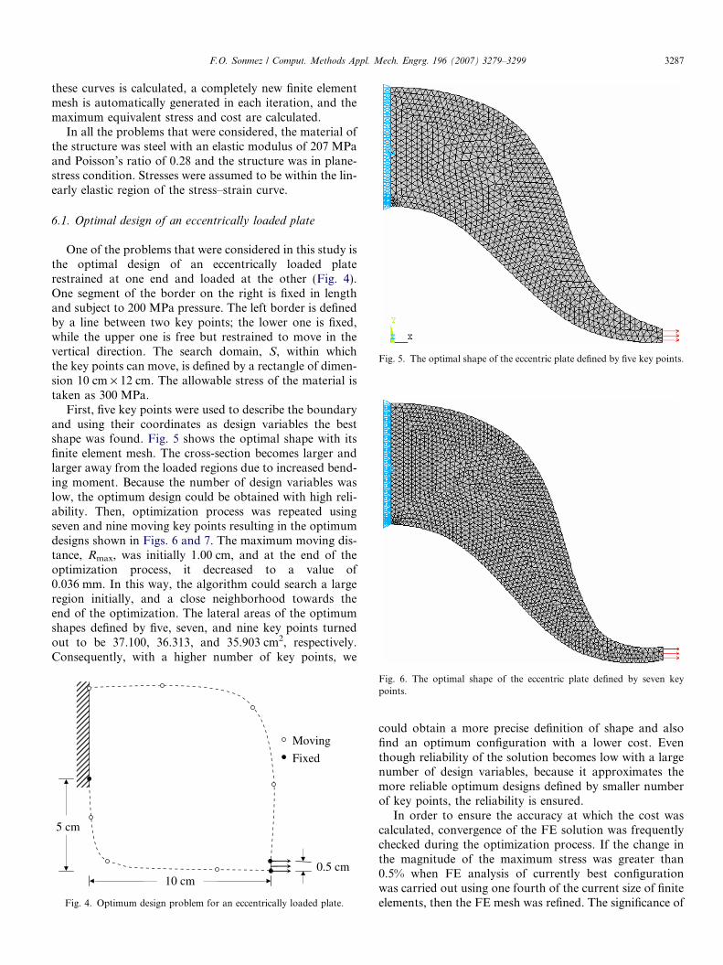
Fig. 5. The optimal shape of the eccentric plate defined by five key points.
F.O. Sonmez / Comput. Methods Appl. Mech. Engrg. 196 (2007) 3279–3299 3287
these curves is calculated, a completely new finite elementmesh is automatically generated in each iteration, and themaximum equivalent stress and cost are calculated.
In all the problems that were considered, the material ofthe structure was steel with an elastic modulus of 207 MPaand Poisson’s ratio of 0.28 and the structure was in plane-stress condition. Stresses were assumed to be within the lin-early elastic region of the stress–strain curve.
6.1. Optimal design of an eccentrically loaded plate
One of the problems that were considered in this study isthe optimal design of an eccentrically loaded platerestrained at one end and loaded at the other (Fig. 4).One segment of the border on the right is fixed in lengthand subject to 200 MPa pressure. The left border is definedby a line between two key points; the lower one is fixed,while the upper one is free but restrained to move in thevertical direction. The search domain, S, within whichthe key points can move, is defined by a rectangle of dimen-sion 10 cm · 12 cm. The allowable stress of the material istaken as 300 MPa.
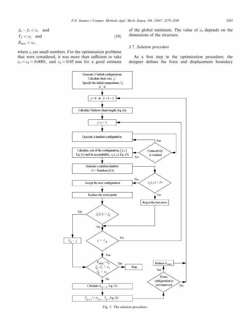
First, five key points were used to describe the boundaryand using their coordinates as design variables the bestshape was found. Fig. 5 shows the optimal shape with itsfinite element mesh. The cross-section becomes larger andlarger away from the loaded regions due to increased bend-ing moment. Because the number of design variables waslow, the optimum design could be obtained with high reli-ability. Then, optimization process was repeated usingseven and nine moving key points resulting in the optimumdesigns shown in Figs. 6 and 7. The maximum moving dis-tance, Rmax, was initially 1.00 cm, and at the end of theoptimization process, it decreased to a value of0.036 mm. In this way, the algorithm could search a largeregion initially, and a close neighborhood towards theend of the optimization. The lateral areas of the optimumshapes defined by five, seven, and nine key points turnedout to be 37.100, 36.313, and 35.903 cm2, respectively.Consequently, with a higher number of key points, we
Moving
Fixed
5 cm
10 cm 0.5 cm
Fig. 4. Optimum design problem for an eccentrically loaded plate.
Fig. 6. The optimal shape of the eccentric plate defined by seven keypoints.
could obtain a more precise definition of shape and alsofind an optimum configuration with a lower cost. Eventhough reliability of the solution becomes low with a largenumber of design variables, because it approximates themore reliable optimum designs defined by smaller numberof key points, the reliability is ensured.
In order to ensure the accuracy at which the cost wascalculated, convergence of the FE solution was frequentlychecked during the optimization process. If the change inthe magnitude of the maximum stress was greater than0.5% when FE analysis of currently best configurationwas carried out using one fourth of the current size of finiteelements, then the FE mesh was refined. The significance of
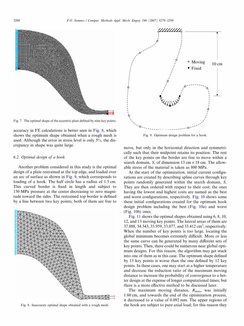
Fig. 7. The optimal shape of the eccentric plate defined by nine key points.
10 cm Moving
Fixed
Fig. 9. Optimum design problem for a hook.
3288 F.O. Sonmez / Comput. Methods Appl. Mech. Engrg. 196 (2007) 3279–3299
accuracy in FE calculations is better seen in Fig. 8, whichshows the optimum shape obtained when a rough mesh isused. Although the error in stress level is only 5%, the dis-crepancy in shape was quite large.
6.2. Optimal design of a hook
Another problem considered in this study is the optimaldesign of a plate restrained at the top edge, and loaded overan arc of surface as shown in Fig. 9, which corresponds toloading of a hook. The half circle has a radius of 1.5 cm.This curved border is fixed in length and subject to150 MPa pressure at the center decreasing to zero magni-tude toward the sides. The restrained top border is definedby a line between two key points; both of them are free to
Fig. 8. Inaccurate optimal shape obtained with a rough mesh.
move, but only in the horizontal direction and symmetri-cally such that their midpoint retains its position. The restof the key points on the border are free to move within asearch domain, S, of dimension 13 cm · 18 cm. The allow-able stress of the material is taken as 800 MPa.
At the start of the optimization, initial current configu-rations are created by describing spline curves through keypoints randomly generated within the search domain, S.They are then ordered with respect to their cost; the oneshaving the lowest and highest costs are named as the bestand worst configurations, respectively. Fig. 10 shows somethese initial configurations created for the optimum hookdesign problem including the best (Fig. 10a) and worst(Fig. 10b) ones.
Fig. 11 shows the optimal shapes obtained using 6, 8, 10,12, and 13 moving key points. The lateral areas of them are37.888, 34.343, 33.959, 33.077, and 33.412 cm2, respectively.When the number of key points is too large, locating theglobal minimum becomes extremely difficult. More or lessthe same curve can be generated by many different sets ofkey points. Then, there could be numerous near global opti-mum designs. For this reason, the algorithm may get stuckinto one of them as in this case. The optimum shape definedby 13 key points is worse than the one defined by 12 keypoints. In these cases, one may start at a higher temperatureand decrease the reduction ratio of the maximum movingdistance to increase the probability of convergence to a bet-ter design at the expense of longer computational times; butthere is a more effective method to be discussed later.
The maximum moving distance, Rmax, was initially1.60 cm, and towards the end of the optimization process,it decreased to a value of 0.092 mm. The upper regions ofthe hook are subject to pure axial load; for this reason they
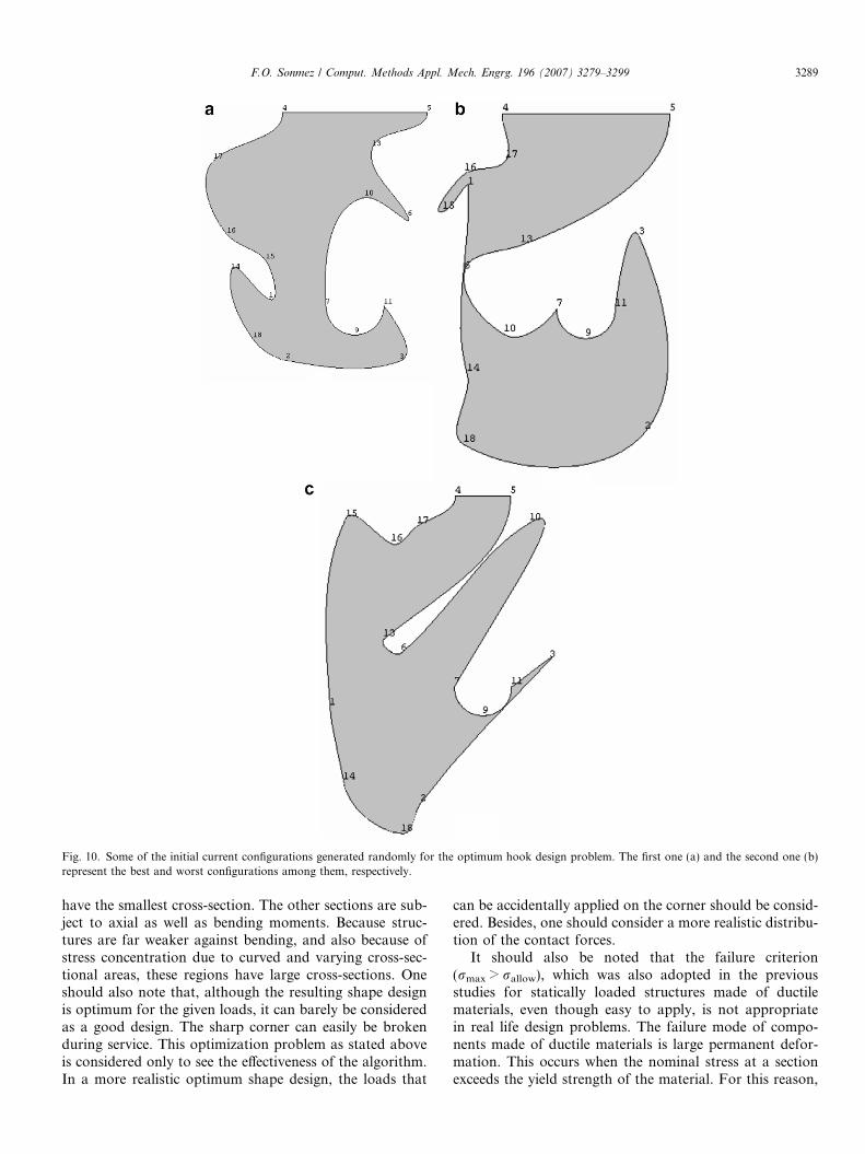
Fig. 10. Some of the initial current configurations generated randomly for the optimum hook design problem. The first one (a) and the second one (b)represent the best and worst configurations among them, respectively.
F.O. Sonmez / Comput. Methods Appl. Mech. Engrg. 196 (2007) 3279–3299 3289
have the smallest cross-section. The other sections are sub-ject to axial as well as bending moments. Because struc-tures are far weaker against bending, and also because ofstress concentration due to curved and varying cross-sec-tional areas, these regions have large cross-sections. Oneshould also note that, although the resulting shape designis optimum for the given loads, it can barely be consideredas a good design. The sharp corner can easily be brokenduring service. This optimization problem as stated aboveis considered only to see the effectiveness of the algorithm.In a more realistic optimum shape design, the loads that
can be accidentally applied on the corner should be consid-ered. Besides, one should consider a more realistic distribu-tion of the contact forces.
It should also be noted that the failure criterion(rmax > rallow), which was also adopted in the previousstudies for statically loaded structures made of ductilematerials, even though easy to apply, is not appropriatein real life design problems. The failure mode of compo-nents made of ductile materials is large permanent defor-mation. This occurs when the nominal stress at a sectionexceeds the yield strength of the material. For this reason,
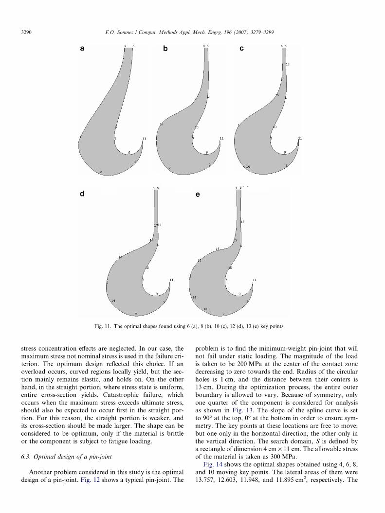
Fig. 11. The optimal shapes found using 6 (a), 8 (b), 10 (c), 12 (d), 13 (e) key points.
3290 F.O. Sonmez / Comput. Methods Appl. Mech. Engrg. 196 (2007) 3279–3299
stress concentration effects are neglected. In our case, themaximum stress not nominal stress is used in the failure cri-terion. The optimum design reflected this choice. If anoverload occurs, curved regions locally yield, but the sec-tion mainly remains elastic, and holds on. On the otherhand, in the straight portion, where stress state is uniform,entire cross-section yields. Catastrophic failure, whichoccurs when the maximum stress exceeds ultimate stress,should also be expected to occur first in the straight por-tion. For this reason, the straight portion is weaker, andits cross-section should be made larger. The shape can beconsidered to be optimum, only if the material is brittleor the component is subject to fatigue loading.
6.3. Optimal design of a pin-joint
Another problem considered in this study is the optimaldesign of a pin-joint. Fig. 12 shows a typical pin-joint. The
problem is to find the minimum-weight pin-joint that willnot fail under static loading. The magnitude of the loadis taken to be 200 MPa at the center of the contact zonedecreasing to zero towards the end. Radius of the circularholes is 1 cm, and the distance between their centers is13 cm. During the optimization process, the entire outerboundary is allowed to vary. Because of symmetry, onlyone quarter of the component is considered for analysisas shown in Fig. 13. The slope of the spline curve is setto 90� at the top, 0� at the bottom in order to ensure sym-metry. The key points at these locations are free to move;but one only in the horizontal direction, the other only inthe vertical direction. The search domain, S is defined bya rectangle of dimension 4 cm · 11 cm. The allowable stressof the material is taken as 300 MPa.
Fig. 14 shows the optimal shapes obtained using 4, 6, 8,and 10 moving key points. The lateral areas of them were13.757, 12.603, 11.948, and 11.895 cm2, respectively. The
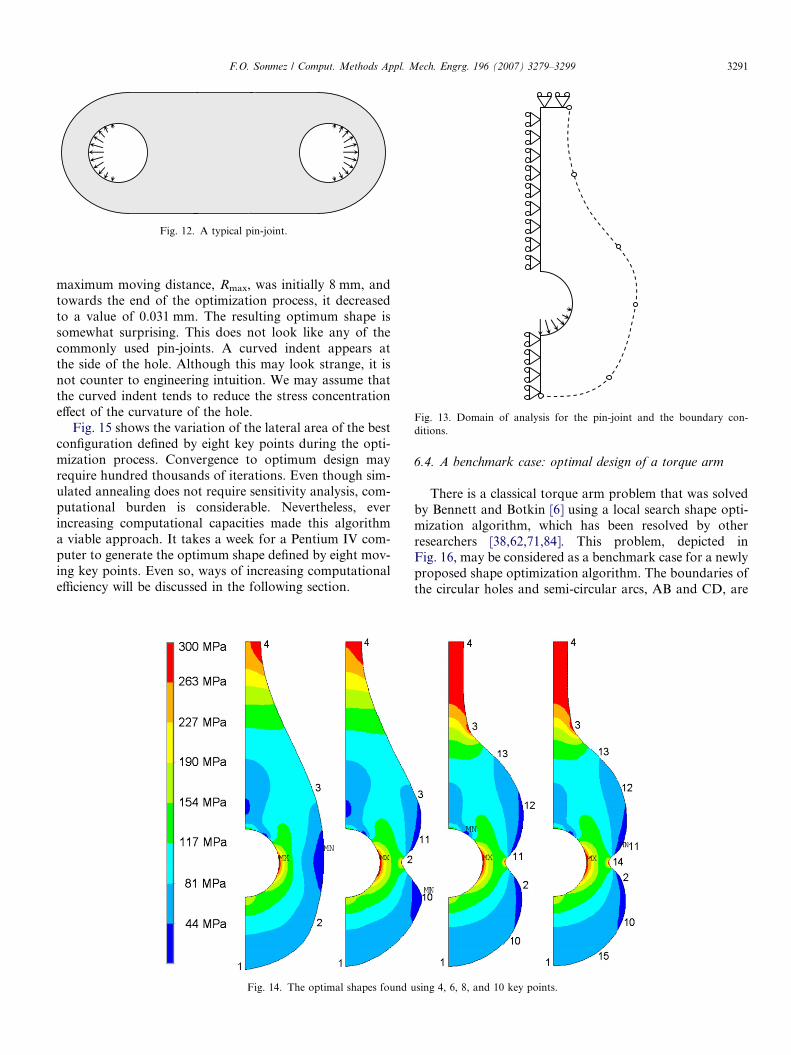
Fig. 12. A typical pin-joint.
Fig. 13. Domain of analysis for the pin-joint and the boundary con-ditions.
F.O. Sonmez / Comput. Methods Appl. Mech. Engrg. 196 (2007) 3279–3299 3291
maximum moving distance, Rmax, was initially 8 mm, andtowards the end of the optimization process, it decreasedto a value of 0.031 mm. The resulting optimum shape issomewhat surprising. This does not look like any of thecommonly used pin-joints. A curved indent appears atthe side of the hole. Although this may look strange, it isnot counter to engineering intuition. We may assume thatthe curved indent tends to reduce the stress concentrationeffect of the curvature of the hole.
Fig. 15 shows the variation of the lateral area of the bestconfiguration defined by eight key points during the opti-mization process. Convergence to optimum design mayrequire hundred thousands of iterations. Even though sim-ulated annealing does not require sensitivity analysis, com-putational burden is considerable. Nevertheless, everincreasing computational capacities made this algorithma viable approach. It takes a week for a Pentium IV com-puter to generate the optimum shape defined by eight mov-ing key points. Even so, ways of increasing computationalefficiency will be discussed in the following section.
Fig. 14. The optimal shapes found u
6.4. A benchmark case: optimal design of a torque arm
There is a classical torque arm problem that was solvedby Bennett and Botkin [6] using a local search shape opti-mization algorithm, which has been resolved by otherresearchers [38,62,71,84]. This problem, depicted inFig. 16, may be considered as a benchmark case for a newlyproposed shape optimization algorithm. The boundaries ofthe circular holes and semi-circular arcs, AB and CD, are
sing 4, 6, 8, and 10 key points.
0 100 200 300 400 500Iteration (thousands)
10
11
12
13
14
15
16
17
18
Area
(cm
2 )
Fig. 15. The change in the lateral area of the best configuration throughthe optimization process.
54.2
40
25
42.7
420
AC
Dimensions are in mm
5066 N
2789 N
R1 R2
BD
Fig. 16. The classical optimum shape design problem for a torque arm.
3292 F.O. Sonmez / Comput. Methods Appl. Mech. Engrg. 196 (2007) 3279–3299
not movable. The points A and C, which are not movable,are connected by a spline curve with two moving keypoints. The inner hole is defined by two semi-circular arcsand two straight lines. The radii of the curvatures and theabscissas of their centers are design variables. Togetherwith the coordinates of the key points on the spline curve,the total number of the design variables is eight. The struc-ture is symmetric with respect to the axis passing throughthe centers of the holes. Its thickness is 3 mm. The allow-able stress of the material is 800 MPa. The boundary ofthe circular hole on the left is restrained from displacing,while the other is loaded as shown. The 2D model is gener-ated by subtracting the areas of the circular holes and mid-dle hole from the area enclosed by the outer boundary.
Fig. 17. The optimal shap
After the area subtraction, if the number of distinct areasis greater than one, connectivity is assumed to be lost.
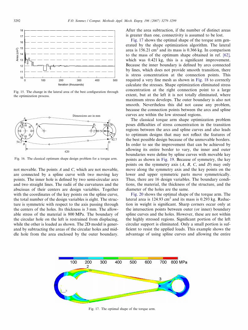
Fig. 17 shows the optimal shape of the torque arm gen-erated by the shape optimization algorithm. The lateralarea is 156.21 cm2 and its mass is 0.366 kg. In comparisonto the mass of the optimum shape obtained in ref. [62],which was 0.421 kg, this is a significant improvement.Because the inner boundary is defined by arcs connectedby lines, which does not provide smooth transition, thereis stress concentration at the connection points. Thisrequired a very fine mesh as shown in Fig. 18 to correctlycalculate the stresses. Shape optimization eliminated stressconcentration at the right connection point to a largeextent, but at the left it is not totally eliminated, wheremaximum stress develops. The outer boundary is also notsmooth. Nevertheless this did not cause any problem,because the connection points between the arcs and splinecurves are within the low stressed regions.
The classical torque arm shape optimization problemposes difficulties of stress concentration in the transitionregions between the arcs and spline curves and also leadsto optimum designs that may not reflect the features ofthe best possible design because of the unmovable borders.In order to see the improvement that can be achieved byallowing its entire border to vary, the inner and outerboundaries were define by spline curves with movable keypoints as shown in Fig. 19. Because of symmetry, the keypoints on the symmetry axis (A, B, C, and D) may onlymove along the symmetry axis and the key points on thelower and upper symmetric parts move symmetrically.Thus, there are 16 design variables. The boundary condi-tions, the material, the thickness of the structure, and thediameter of the holes are the same.
Fig. 20 shows the optimal shape of the torque arm. Thelateral area is 124.93 cm2 and its mass is 0.293 kg. Reduc-tion in weight is significant. Sharp corners occur only atthe intersection points between outer (or inner) boundaryspline curves and the holes. However, these are not withinthe highly stressed regions. Significant portion of the leftcircular support is eliminated. Only a small portion is suf-ficient to resist the applied loads. This example shows theadvantage of using spline curves and allowing the entire
e of the torque arm.
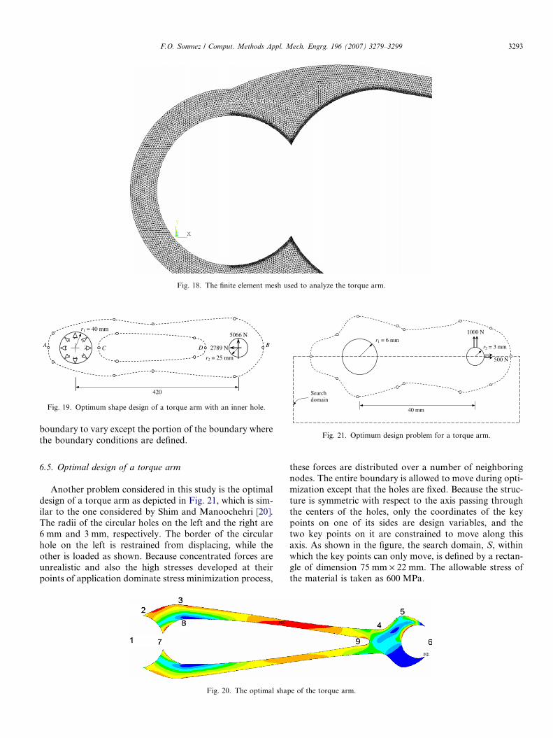
Fig. 18. The finite element mesh used to analyze the torque arm.
r1 = 40 mm
420
A C
5066 N
2789 N BD
r2 = 25 mm
Fig. 19. Optimum shape design of a torque arm with an inner hole. 40 mm
r1 = 6 mm r2 = 3 mm
500 N
Searchdomain
1000 N
Fig. 21. Optimum design problem for a torque arm.
F.O. Sonmez / Comput. Methods Appl. Mech. Engrg. 196 (2007) 3279–3299 3293
boundary to vary except the portion of the boundary wherethe boundary conditions are defined.
6.5. Optimal design of a torque arm
Another problem considered in this study is the optimaldesign of a torque arm as depicted in Fig. 21, which is sim-ilar to the one considered by Shim and Manoochehri [20].The radii of the circular holes on the left and the right are6 mm and 3 mm, respectively. The border of the circularhole on the left is restrained from displacing, while theother is loaded as shown. Because concentrated forces areunrealistic and also the high stresses developed at theirpoints of application dominate stress minimization process,
Fig. 20. The optimal shap
these forces are distributed over a number of neighboringnodes. The entire boundary is allowed to move during opti-mization except that the holes are fixed. Because the struc-ture is symmetric with respect to the axis passing throughthe centers of the holes, only the coordinates of the keypoints on one of its sides are design variables, and thetwo key points on it are constrained to move along thisaxis. As shown in the figure, the search domain, S, withinwhich the key points can only move, is defined by a rectan-gle of dimension 75 mm · 22 mm. The allowable stress ofthe material is taken as 600 MPa.
e of the torque arm.
3294 F.O. Sonmez / Comput. Methods Appl. Mech. Engrg. 196 (2007) 3279–3299
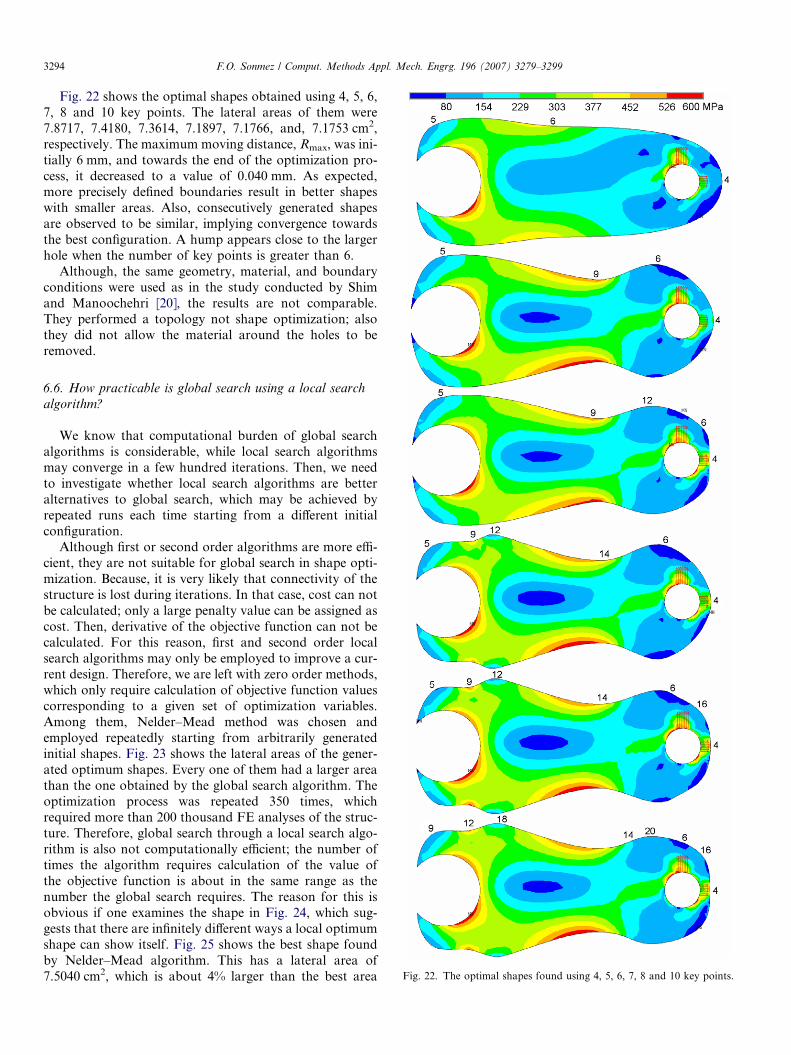
Fig. 22 shows the optimal shapes obtained using 4, 5, 6,7, 8 and 10 key points. The lateral areas of them were7.8717, 7.4180, 7.3614, 7.1897, 7.1766, and, 7.1753 cm2,respectively. The maximum moving distance, Rmax, was ini-tially 6 mm, and towards the end of the optimization pro-cess, it decreased to a value of 0.040 mm. As expected,more precisely defined boundaries result in better shapeswith smaller areas. Also, consecutively generated shapesare observed to be similar, implying convergence towardsthe best configuration. A hump appears close to the largerhole when the number of key points is greater than 6.
Although, the same geometry, material, and boundaryconditions were used as in the study conducted by Shimand Manoochehri [20], the results are not comparable.They performed a topology not shape optimization; alsothey did not allow the material around the holes to beremoved.
Fig. 22. The optimal shapes found using 4, 5, 6, 7, 8 and 10 key points.
6.6. How practicable is global search using a local search
algorithm?
We know that computational burden of global searchalgorithms is considerable, while local search algorithmsmay converge in a few hundred iterations. Then, we needto investigate whether local search algorithms are betteralternatives to global search, which may be achieved byrepeated runs each time starting from a different initialconfiguration.
Although first or second order algorithms are more effi-cient, they are not suitable for global search in shape opti-mization. Because, it is very likely that connectivity of thestructure is lost during iterations. In that case, cost can notbe calculated; only a large penalty value can be assigned ascost. Then, derivative of the objective function can not becalculated. For this reason, first and second order localsearch algorithms may only be employed to improve a cur-rent design. Therefore, we are left with zero order methods,which only require calculation of objective function valuescorresponding to a given set of optimization variables.Among them, Nelder–Mead method was chosen andemployed repeatedly starting from arbitrarily generatedinitial shapes. Fig. 23 shows the lateral areas of the gener-ated optimum shapes. Every one of them had a larger areathan the one obtained by the global search algorithm. Theoptimization process was repeated 350 times, whichrequired more than 200 thousand FE analyses of the struc-ture. Therefore, global search through a local search algo-rithm is also not computationally efficient; the number oftimes the algorithm requires calculation of the value ofthe objective function is about in the same range as thenumber the global search requires. The reason for this isobvious if one examines the shape in Fig. 24, which sug-gests that there are infinitely different ways a local optimumshape can show itself. Fig. 25 shows the best shape foundby Nelder–Mead algorithm. This has a lateral area of7.5040 cm2, which is about 4% larger than the best area
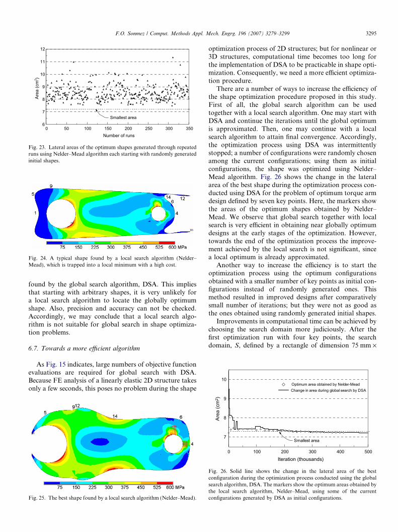
Fig. 24. A typical shape found by a local search algorithm (Nelder–Mead), which is trapped into a local minimum with a high cost.
10Optimum area obtained by Nelder-MeadChange in area during global search by DSA
0 50 100 150 200 250 300 350Number of runs
6
7
8
9
10
11
12
Area
(cm
2 )
Smallest area
Fig. 23. Lateral areas of the optimum shapes generated through repeatedruns using Nelder–Mead algorithm each starting with randomly generatedinitial shapes.
F.O. Sonmez / Comput. Methods Appl. Mech. Engrg. 196 (2007) 3279–3299 3295
found by the global search algorithm, DSA. This impliesthat starting with arbitrary shapes, it is very unlikely fora local search algorithm to locate the globally optimumshape. Also, precision and accuracy can not be checked.Accordingly, we may conclude that a local search algo-rithm is not suitable for global search in shape optimiza-tion problems.
6.7. Towards a more efficient algorithm
As Fig. 15 indicates, large numbers of objective functionevaluations are required for global search with DSA.Because FE analysis of a linearly elastic 2D structure takesonly a few seconds, this poses no problem during the shape
Fig. 25. The best shape found by a local search algorithm (Nelder–Mead).
optimization process of 2D structures; but for nonlinear or3D structures, computational time becomes too long forthe implementation of DSA to be practicable in shape opti-mization. Consequently, we need a more efficient optimiza-tion procedure.
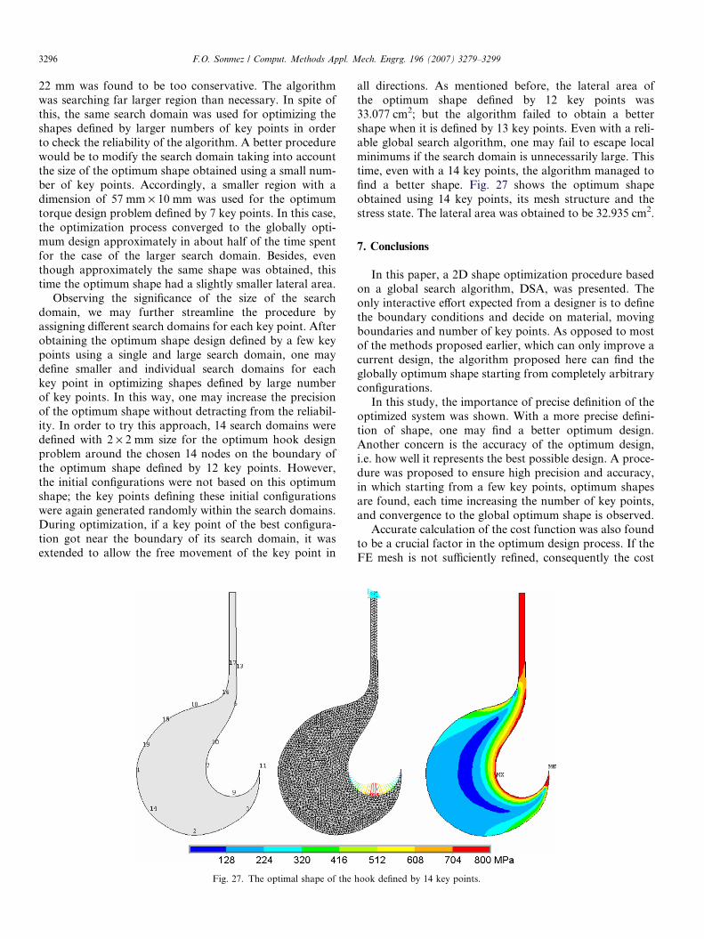
There are a number of ways to increase the efficiency ofthe shape optimization procedure proposed in this study.First of all, the global search algorithm can be usedtogether with a local search algorithm. One may start withDSA and continue the iterations until the global optimumis approximated. Then, one may continue with a localsearch algorithm to attain final convergence. Accordingly,the optimization process using DSA was intermittentlystopped; a number of configurations were randomly chosenamong the current configurations; using them as initialconfigurations, the shape was optimized using Nelder–Mead algorithm. Fig. 26 shows the change in the lateralarea of the best shape during the optimization process con-ducted using DSA for the problem of optimum torque armdesign defined by seven key points. Here, the markers showthe areas of the optimum shapes obtained by Nelder–Mead. We observe that global search together with localsearch is very efficient in obtaining near globally optimumdesigns at the early stages of the optimization. However,towards the end of the optimization process the improve-ment achieved by the local search is not significant, sincea local optimum is already approximated.
Another way to increase the efficiency is to start theoptimization process using the optimum configurationsobtained with a smaller number of key points as initial con-figurations instead of randomly generated ones. Thismethod resulted in improved designs after comparativelysmall number of iterations; but they were not as good asthe ones obtained using randomly generated initial shapes.
Improvements in computational time can be achieved bychoosing the search domain more judiciously. After thefirst optimization run with four key points, the searchdomain, S, defined by a rectangle of dimension 75 mm ·
0 100 200 300 400 500Iteration (thousands)
7
8
9
Area
(cm
2 )
Smallest area
Fig. 26. Solid line shows the change in the lateral area of the bestconfiguration during the optimization process conducted using the globalsearch algorithm, DSA. The markers show the optimum areas obtained bythe local search algorithm, Nelder–Mead, using some of the currentconfigurations generated by DSA as initial configurations.
3296 F.O. Sonmez / Comput. Methods Appl. Mech. Engrg. 196 (2007) 3279–3299
22 mm was found to be too conservative. The algorithmwas searching far larger region than necessary. In spite ofthis, the same search domain was used for optimizing theshapes defined by larger numbers of key points in orderto check the reliability of the algorithm. A better procedurewould be to modify the search domain taking into accountthe size of the optimum shape obtained using a small num-ber of key points. Accordingly, a smaller region with adimension of 57 mm · 10 mm was used for the optimumtorque design problem defined by 7 key points. In this case,the optimization process converged to the globally opti-mum design approximately in about half of the time spentfor the case of the larger search domain. Besides, eventhough approximately the same shape was obtained, thistime the optimum shape had a slightly smaller lateral area.
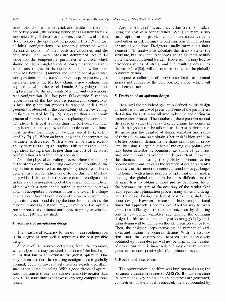
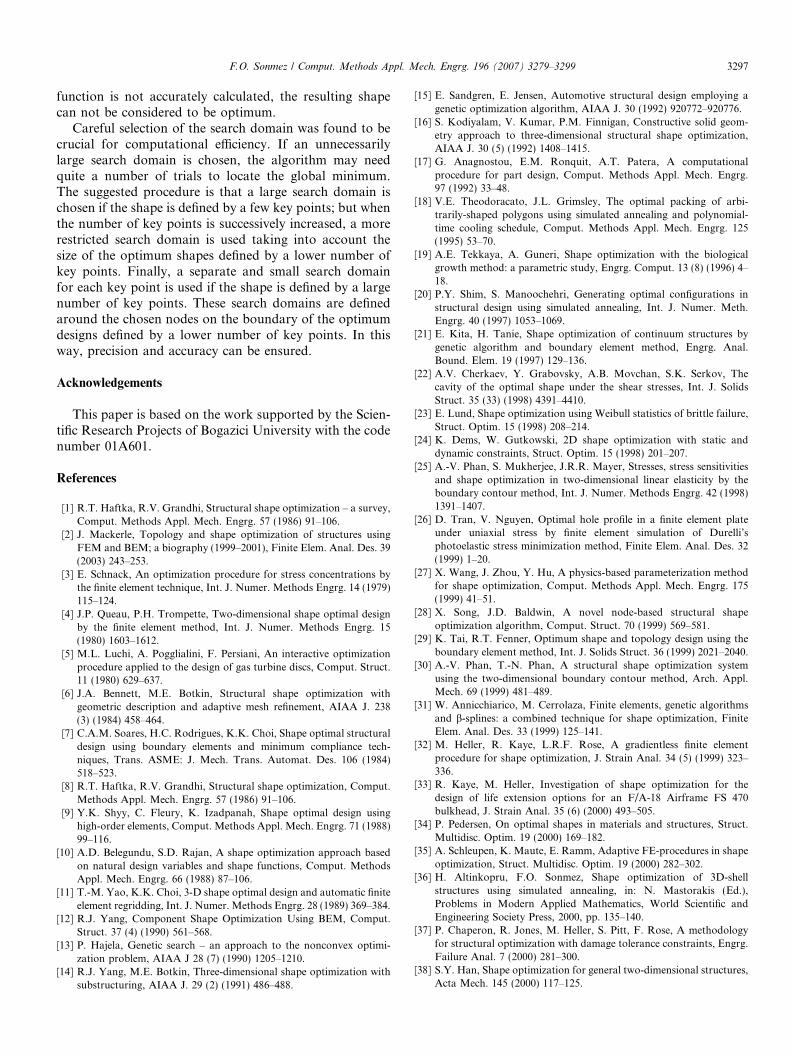
Observing the significance of the size of the searchdomain, we may further streamline the procedure byassigning different search domains for each key point. Afterobtaining the optimum shape design defined by a few keypoints using a single and large search domain, one maydefine smaller and individual search domains for eachkey point in optimizing shapes defined by large numberof key points. In this way, one may increase the precisionof the optimum shape without detracting from the reliabil-ity. In order to try this approach, 14 search domains weredefined with 2 · 2 mm size for the optimum hook designproblem around the chosen 14 nodes on the boundary ofthe optimum shape defined by 12 key points. However,the initial configurations were not based on this optimumshape; the key points defining these initial configurationswere again generated randomly within the search domains.During optimization, if a key point of the best configura-tion got near the boundary of its search domain, it wasextended to allow the free movement of the key point in
Fig. 27. The optimal shape of the
all directions. As mentioned before, the lateral area ofthe optimum shape defined by 12 key points was33.077 cm2; but the algorithm failed to obtain a bettershape when it is defined by 13 key points. Even with a reli-able global search algorithm, one may fail to escape localminimums if the search domain is unnecessarily large. Thistime, even with a 14 key points, the algorithm managed tofind a better shape. Fig. 27 shows the optimum shapeobtained using 14 key points, its mesh structure and thestress state. The lateral area was obtained to be 32.935 cm2.
7. Conclusions
In this paper, a 2D shape optimization procedure basedon a global search algorithm, DSA, was presented. Theonly interactive effort expected from a designer is to definethe boundary conditions and decide on material, movingboundaries and number of key points. As opposed to mostof the methods proposed earlier, which can only improve acurrent design, the algorithm proposed here can find theglobally optimum shape starting from completely arbitraryconfigurations.
In this study, the importance of precise definition of theoptimized system was shown. With a more precise defini-tion of shape, one may find a better optimum design.Another concern is the accuracy of the optimum design,i.e. how well it represents the best possible design. A proce-dure was proposed to ensure high precision and accuracy,in which starting from a few key points, optimum shapesare found, each time increasing the number of key points,and convergence to the global optimum shape is observed.
Accurate calculation of the cost function was also foundto be a crucial factor in the optimum design process. If theFE mesh is not sufficiently refined, consequently the cost
hook defined by 14 key points.
F.O. Sonmez / Comput. Methods Appl. Mech. Engrg. 196 (2007) 3279–3299 3297
function is not accurately calculated, the resulting shapecan not be considered to be optimum.
Careful selection of the search domain was found to becrucial for computational efficiency. If an unnecessarilylarge search domain is chosen, the algorithm may needquite a number of trials to locate the global minimum.The suggested procedure is that a large search domain ischosen if the shape is defined by a few key points; but whenthe number of key points is successively increased, a morerestricted search domain is used taking into account thesize of the optimum shapes defined by a lower number ofkey points. Finally, a separate and small search domainfor each key point is used if the shape is defined by a largenumber of key points. These search domains are definedaround the chosen nodes on the boundary of the optimumdesigns defined by a lower number of key points. In thisway, precision and accuracy can be ensured.
Acknowledgements
This paper is based on the work supported by the Scien-tific Research Projects of Bogazici University with the codenumber 01A601.
References
[1] R.T. Haftka, R.V. Grandhi, Structural shape optimization – a survey,Comput. Methods Appl. Mech. Engrg. 57 (1986) 91–106.
[2] J. Mackerle, Topology and shape optimization of structures usingFEM and BEM; a biography (1999–2001), Finite Elem. Anal. Des. 39(2003) 243–253.
[3] E. Schnack, An optimization procedure for stress concentrations bythe finite element technique, Int. J. Numer. Methods Engrg. 14 (1979)115–124.
[4] J.P. Queau, P.H. Trompette, Two-dimensional shape optimal designby the finite element method, Int. J. Numer. Methods Engrg. 15(1980) 1603–1612.
[5] M.L. Luchi, A. Pogglialini, F. Persiani, An interactive optimizationprocedure applied to the design of gas turbine discs, Comput. Struct.11 (1980) 629–637.
[6] J.A. Bennett, M.E. Botkin, Structural shape optimization withgeometric description and adaptive mesh refinement, AIAA J. 238(3) (1984) 458–464.
[7] C.A.M. Soares, H.C. Rodrigues, K.K. Choi, Shape optimal structuraldesign using boundary elements and minimum compliance tech-niques, Trans. ASME: J. Mech. Trans. Automat. Des. 106 (1984)518–523.
[8] R.T. Haftka, R.V. Grandhi, Structural shape optimization, Comput.Methods Appl. Mech. Engrg. 57 (1986) 91–106.
[9] Y.K. Shyy, C. Fleury, K. Izadpanah, Shape optimal design usinghigh-order elements, Comput. Methods Appl. Mech. Engrg. 71 (1988)99–116.
[10] A.D. Belegundu, S.D. Rajan, A shape optimization approach basedon natural design variables and shape functions, Comput. MethodsAppl. Mech. Engrg. 66 (1988) 87–106.
[11] T.-M. Yao, K.K. Choi, 3-D shape optimal design and automatic finiteelement regridding, Int. J. Numer. Methods Engrg. 28 (1989) 369–384.
[12] R.J. Yang, Component Shape Optimization Using BEM, Comput.Struct. 37 (4) (1990) 561–568.
[13] P. Hajela, Genetic search – an approach to the nonconvex optimi-zation problem, AIAA J 28 (7) (1990) 1205–1210.
[14] R.J. Yang, M.E. Botkin, Three-dimensional shape optimization withsubstructuring, AIAA J. 29 (2) (1991) 486–488.
[15] E. Sandgren, E. Jensen, Automotive structural design employing agenetic optimization algorithm, AIAA J. 30 (1992) 920772–920776.
[16] S. Kodiyalam, V. Kumar, P.M. Finnigan, Constructive solid geom-etry approach to three-dimensional structural shape optimization,AIAA J. 30 (5) (1992) 1408–1415.
[17] G. Anagnostou, E.M. Ronquit, A.T. Patera, A computationalprocedure for part design, Comput. Methods Appl. Mech. Engrg.97 (1992) 33–48.
[18] V.E. Theodoracato, J.L. Grimsley, The optimal packing of arbi-trarily-shaped polygons using simulated annealing and polynomial-time cooling schedule, Comput. Methods Appl. Mech. Engrg. 125(1995) 53–70.
[19] A.E. Tekkaya, A. Guneri, Shape optimization with the biologicalgrowth method: a parametric study, Engrg. Comput. 13 (8) (1996) 4–18.
[20] P.Y. Shim, S. Manoochehri, Generating optimal configurations instructural design using simulated annealing, Int. J. Numer. Meth.Engrg. 40 (1997) 1053–1069.
[21] E. Kita, H. Tanie, Shape optimization of continuum structures bygenetic algorithm and boundary element method, Engrg. Anal.Bound. Elem. 19 (1997) 129–136.
[22] A.V. Cherkaev, Y. Grabovsky, A.B. Movchan, S.K. Serkov, Thecavity of the optimal shape under the shear stresses, Int. J. SolidsStruct. 35 (33) (1998) 4391–4410.
[23] E. Lund, Shape optimization using Weibull statistics of brittle failure,Struct. Optim. 15 (1998) 208–214.
[24] K. Dems, W. Gutkowski, 2D shape optimization with static anddynamic constraints, Struct. Optim. 15 (1998) 201–207.
[25] A.-V. Phan, S. Mukherjee, J.R.R. Mayer, Stresses, stress sensitivitiesand shape optimization in two-dimensional linear elasticity by theboundary contour method, Int. J. Numer. Methods Engrg. 42 (1998)1391–1407.
[26] D. Tran, V. Nguyen, Optimal hole profile in a finite element plateunder uniaxial stress by finite element simulation of Durelli’sphotoelastic stress minimization method, Finite Elem. Anal. Des. 32(1999) 1–20.
[27] X. Wang, J. Zhou, Y. Hu, A physics-based parameterization methodfor shape optimization, Comput. Methods Appl. Mech. Engrg. 175(1999) 41–51.
[28] X. Song, J.D. Baldwin, A novel node-based structural shapeoptimization algorithm, Comput. Struct. 70 (1999) 569–581.
[29] K. Tai, R.T. Fenner, Optimum shape and topology design using theboundary element method, Int. J. Solids Struct. 36 (1999) 2021–2040.
[30] A.-V. Phan, T.-N. Phan, A structural shape optimization systemusing the two-dimensional boundary contour method, Arch. Appl.Mech. 69 (1999) 481–489.
[31] W. Annicchiarico, M. Cerrolaza, Finite elements, genetic algorithmsand b-splines: a combined technique for shape optimization, FiniteElem. Anal. Des. 33 (1999) 125–141.
[32] M. Heller, R. Kaye, L.R.F. Rose, A gradientless finite elementprocedure for shape optimization, J. Strain Anal. 34 (5) (1999) 323–336.
[33] R. Kaye, M. Heller, Investigation of shape optimization for thedesign of life extension options for an F/A-18 Airframe FS 470bulkhead, J. Strain Anal. 35 (6) (2000) 493–505.
[34] P. Pedersen, On optimal shapes in materials and structures, Struct.Multidisc. Optim. 19 (2000) 169–182.
[35] A. Schleupen, K. Maute, E. Ramm, Adaptive FE-procedures in shapeoptimization, Struct. Multidisc. Optim. 19 (2000) 282–302.
[36] H. Altinkopru, F.O. Sonmez, Shape optimization of 3D-shellstructures using simulated annealing, in: N. Mastorakis (Ed.),Problems in Modern Applied Mathematics, World Scientific andEngineering Society Press, 2000, pp. 135–140.
[37] P. Chaperon, R. Jones, M. Heller, S. Pitt, F. Rose, A methodologyfor structural optimization with damage tolerance constraints, Engrg.Failure Anal. 7 (2000) 281–300.
[38] S.Y. Han, Shape optimization for general two-dimensional structures,Acta Mech. 145 (2000) 117–125.
3298 F.O. Sonmez / Comput. Methods Appl. Mech. Engrg. 196 (2007) 3279–3299
[39] J. Herskovits, G. Dias, G. Santos, C.M.M. Soares, Shape structuraloptimization with an interior point nonlinear programming algo-rithm, Struct. Multidisc. Optim. 20 (2000) 107–115.
[40] J. Herskovits, A. Leontiev, G. Dias, G. Santos, C.M.M. Soares,Contact shape optimization: a bilevel programming approach, Struct.Multidisc. Optim. 20 (2000) 214–221.
[41] M. Cerrolaza, W. Annicchiarico, M. Martinez, Optimization of 2Dboundary element models Using b-splines and genetic algorithms,Engrg. Anal. Bound. Elem. 24 (2000) 427–440.
[42] M. Kegl, Shape optimal design of structures: an efficient shaperepresentation concept, Int. J. Numer. Methods Engrg. 49 (2000)1571–1588.
[43] W. Waldman, M. Heller, G.X. Chen, Optimal free-form shapes forshoulder fillets in flat plates under tension and bending, Int. J. Fatigue23 (2001) 509–523.
[44] P. Vinot, S. Cogan, J. Piranda, Shape optimization of thin-walledbeam-like structures, Thin-walled Struct. 39 (2001) 611–630.
[45] N. Gunduz, N. Akbulut, F.O. Sonmez, Generating optimal 2Dstructural designs using simulated annealing, in: S. Hernandez, C.A.Brebbia (Eds.), Computer Aided Optimum Design of Structures, vol.VII, WIT Press, 2001, pp. 347–356.
[46] D. Hilding, B. Torstenfelt, A. Klarbring, A computational method-ology for shape optimization of structures in frictionlesscontact, Comput. Methods Appl. Mech. Engrg. 190 (2001) 4043–4060.
[47] W. Annicchiarico, M. Cerrolaza, Structural shape optimization 3Dfinite-element models based on genetic algorithms and geometricmodeling, Finite Elem. Anal. Des. 37 (2001) 403–415.
[48] S.Y. Woon, O.M. Querin, G.P. Steven, Structural application of ashape optimization method based on a genetic algorithm, Struct.Multidisc. Optim. 22 (2001) 57–64.
[49] L. Qing, G.P. Steven, O.M. Querin, Y.M. Xie, Stress basedoptimization of torsional shafts using and evolutionary procedure,Int. J. Solids Struct. 38 (2001) 5661–5677.
[50] H.S. Hedia, Shape optimisation to maximize crack initiation time,Bio-Medical Mater. Engrg. 11 (2001) 293–300.
[51] F. Bobaru, S. Mukherjee, Shape sensitivity analysis and shapeoptimization in planar elasticity using the element-free Galerkinmethod, Comput. Methods Appl. Mech. Engrg. 190 (2001) 4319–4337.
[52] S. Butkewitsch, V. Steffen, Shape optimization, model updating andempirical modeling applied to the design synthesis of a heavy truckside guard, Int. J. Solids Struct. 39 (2002) 4747–4771.
[53] J.A.T. Freitas, I. Cismasiu, Shape optimization with hybrid – Trefftzdisplacement elements, Int. J. Numer. Methods Engrg. 53 (2002) 473–498.
[54] I. Paczelt, T. Szabo, Solution of contact optimization problems ofcylindrical bodies using HP-FEM, Int. J. Numer. Methods Engrg. 53(2002) 123–146.
[55] S.-Y. Han, J.-K. Lim, Shape optimization for prolonging fatigue life,JSME Int. J.: Ser. A 45 (2) (2002) 298–304.
[56] P. Beremlijski, J. Haslinger, M. Kocvara, J. Outrata, Shape optimi-zation in contact problems with Coulomb friction, Soc. Ind. Appl.Math. 13 (2) (2002) 561–587.
[57] T. Burcynski, A. Dlugosz, Evolutionary optimization in thermoelasticproblems using the boundary element method, Comput. Mech. 28(2002) 317–324.
[58] F. Bobaru, S. Mukherjee, Meshless approach to shape optimizationof linear thermoelastic solids, Struct. Multidisc. Optim. 53 (2002)765–796.
[59] E. Schnack, W. Weikl, Shape optimization under fatigue usingcontinuum damage mechanics, Comput.-Aided Des. 34 (2002) 929–938.
[60] A. Tafreshi, Shape design sensitivity analysis of 2D anisotropicstructures using the boundary element method, Engrg. Anal. Bound.Elem. 26 (2002) 237–251.
[61] J. Lampinen, Cam shape optimization by genetic algorithm, Com-put.-Aided Des. 35 (2003) 727–737.
[62] N.H. Kim, K.K. Choi, M.E. Botkin, Numerical method for shapeoptimization using meshfree method, Struct. Multidisc. Optim. 24(2003) 418–429.
[63] J. Shen, D. Yoon, A new scheme for efficient and direct shapeoptimization of complex structures represented by polygonal meshes,Int. J. Numer. Methods Engrg. 58 (2003) 2201–2223.
[64] S.Y. Woon, L. Tong, O.M. Querin, G.P. Steven, Knowledge-basedalgorithms in fixed-grid GA shape optimization, Int. J. Numer.Methods Engrg. 58 (2003) 643–660.
[65] M. Ozakca, N. Tays�i, F. Kolcu, Buckling analysis and shapeoptimization of elastic variable thickness circular and annularplates – II. Shape optimization, Engrg. Struct. 25 (2003) 193–199.
[66] C. Wessel, A. Cisilino, B. Sensale, Structural shape optimisation usingboundary elements and the biological growth method, Struct.Multidisc. Optim. 28 (2004) 221–227.
[67] S.A. Falco, S.M.B. Afonso, L.E. Vaz, Analysis and optimal design ofplates and shells under dynamic loads – II: optimization, Struct.Multidisc. Optim. 27 (2004) 197–209.
[68] M. McDonald, M. Heller, Robust shape optimization of notches forfatigue-life extension, Struct. Multidisc. Optim. 28 (2004) 55–68.
[69] S. Hyun, C. Kim, J.H. Son, S.H. Shin, Y.S. Kim, An efficient shapeoptimization method based on fem and B-spline curves and shaping atorque converter clutch disk, Finite Elem. Anal. Des. 40 (2004) 1803–1815.
[70] M.J. Garcia, C.A. Gonzales, Shape optimisation of continuumstructures via evolution strategies and fixed grid finite elementanalysis, Struct. Multidisc. Optim. 26 (2004) 92–98.
[71] G.-W. Jang, Y.Y. Kim, K.K. Choi, Remesh-free shape optimizationusing the wavelet-Galerkin method, Int. J. Solids Struct. 41 (2004)6465–6483.
[72] A.A. Mailybaev, H. Yabuno, H. Kaneko, Optimal shapes ofparametrically excited beams, Struct. Multidisc. Optim. 27 (2004)435–445.
[73] J. Norato, R. Haber, D. Tortorelli, M.P. Bendsoe, A geometryprojection method for shape optimization, Int. J. Numer. MethodsEngrg. 60 (2004) 2289–2312.
[74] M. Haiba, D.C. Barton, P.C. Brooks, M.C. Levesley, Evolutionarystructural optimization of dynamically loaded components in con-sideration of fatigue life, Adv. Engrg. Software 36 (2005) 49–57.
[75] W.L. Li, Q. Li, G.P. Steven, Y.M. Xie, An evolutionary shapeoptimization for elastic contact problems subject to multiple loadcases, Comput. Methods Appl. Mech. Engrg. 194 (2005) 3394–3415.
[76] E. Cervera, J. Trevelyan, Evolutionary structural optimization basedon boundary representation of NURBS. Part 1: 2D algorithms,Comput. Struct. 83 (2005) 1902–1916.
[77] F. Schmid, K. Hirschen, S. Meynen, M. Schafer, An enhancedapproach for shape optimization using an adaptive algorithm, FiniteElem. Anal. Des. 41 (2005) 521–543.
[78] J.-S. Liu, G.T. Parks, P.J. Clarkson, Topology/shape optimization ofaxisymmetric continuum structures – a metamorphic developmentapproach, Struct. Multidisc. Optim. 29 (2005) 73–83.
[79] Z.Q. Zhang, J.X. Zhou, N. Zhou, X.M. Wang, L. Zhang, Shapeoptimization using kernel particle method and an enriched geneticalgorithm, Comput. Methods Appl. Mech. Engrg. 194 (2005) 4048–4070.
[80] R. Das, R. Jones, Y.M. Xie, Design of structures for optimal staticstrength Using ESO, Engrg. Failure Anal. 12 (2005) 61–80.
[81] I.Y. Shevtsov, V.L. Markine, C. Esveld, Optimal design of wheelprofile for railway vehicles, Wear 258 (2005) 1022–1030.
[82] M.-H. Chang, C.-H. Cheng, Optimal design of slider shape forsatisfying load demands under specified operation conditions, Tribol.Int. 38 (2005) 757–768.
[83] R. Meske, J. Sauter, E. Schnack, Nonparametric gradient-less shapeoptimization for real-world applications, Struct. Multidisc. Optim. 30(2005) 201–218.
[84] N.H. Kim, Y. Chang, Eulerian shape design sensitivity analysis andoptimization with a fixed grid, Comput. Methods Appl. Mech. Engrg.194 (2005) 3291–3314.

F.O. Sonmez / Comput. Methods Appl. Mech. Engrg. 196 (2007) 3279–3299 3299
[85] R. Jones, D. Peng, P. Chaperon, S. Pitt, D. Abramson, T. Peachey,Structural optimisation with damage tolerance constraints, Theor.Appl. Fract. Mech. 43 (2005) 133–155.
[86] F.O. Sonmez, Precision and accuracy in generating globally optimumshapes, in: I. Garcia, L.G. Casado, E.M.T. Hendrix, B. Toth (Eds.),Proceedings of the International Workshop on Global Optimization,San Jose, Spain, pp. 231–236, 2005.
[87] Z. Wu, An efficient approach for shape optimization of components,Int. J. Mech. Sci. 47 (2005) 1595–1610.
[88] H.H. Yoo, J.E. Cho, J. Chung, Modal analysis and shape optimi-zation of rotating cantilever beams, J. Sound Vibr. 290 (2006) 223–241.
[89] S. Kirkpatrick, C.D. Gelatt, M.P. Vecchi, Optimization by simulatedannealing, Science 220 (1983) 671–680.
[90] M.M. Ali, A. Torn, S. Viitanen, A direct search variant of thesimulated annealing algorithm for optimization involving continuousvariables, Comput. Operat. Res. 29 (2002) 87–102.


