Shape-based coordination in locomotion controlbiorobotics.ri.cmu.edu/papers/paperUploads/Shape-based...
16
Article Shape-based coordination in locomotion control The International Journal of Robotics Research 1–16 © The Author(s) 2018 Reprints and permissions: sagepub.co.uk/journalsPermissions.nav DOI: 10.1177/0278364918761569 journals.sagepub.com/home/ijr Matthew Travers, Julian Whitman and Howie Choset Abstract Highly articulated systems are capable of executing a variety of behaviors by coordinating their many internal degrees of freedom to help them move more effectively in complex terrains. However, this inherent variety poses significant challenges that have been the subject of a great deal of previous work: What are the most effective or most efficient methods for achieving the intrinsic coordination necessary to produce desired global objectives? This work takes these questions one step further, asking how different levels of coordination, which we quantify in terms of kinematic coupling, affect articulated locomotion in environments with different degrees of underlying structure. We introduce shape functions as the analytical basis for specifying kinematic coupling relationships that constrain the relative motion among the internal degrees of freedom for a given system during its nominal locomotion. Furthermore, we show how shape functions are used to derive shape-based controllers (SBCs) that manage the compliant interaction between articulated bodies and the environment while explicitly preserving the inter-joint coupling defined by shape functions. Initial experimental evidence provides a comparison of the benefits of different levels of coordination for two separate platforms in environments with different degrees of inherent structure. The experimental resultsshow that decentralized implementations, where there is relatively little inter-joint coupling, perform well across a spectrum of different terrains but that there are potential benefits to higher degrees of coupling in structured terrains. We discuss how this observation has implications related to future planning and control approaches that actively “tune” their underlying structure by dynamically varying the assumed level of coupling as a function of task specification and local environmental conditions. Keywords Articulated locomotion, compliant control, shape function, kinematic synergies, snake robot, hexapod robot, central pattern generator (CPG), dynamic movement primitive (DMP), admittance control 1. Introduction Whether biological or man made, highly articulated sys- tems are capable of leveraging fixed motion patterns that coordinate their many internal degrees of freedom to help them move more effectively in non-trivial tasks and envi- ronments. In particular, prior work shows that the expres- sive global behaviors of articulated systems can in many cases be represented using low-dimensional parameterized expressions that capture the coordination among their inter- nal degrees of freedom; this has been shown in data col- lected from biological systems (Gong et al., 2014; Santello et al., 1998; Alexandrov et al., 1998; Freitas et al., 2006; Tricon et al., 2007) and has been demonstrated on differ- ent robotic platforms (Hauser et al., 2007, 2011; Ajoudani et al., 2013; Gabiccini et al., 20011; Catalano et al., 2012; Ciocarlie et al., 2007). However, relatively little attention has been paid to evaluating how varying the level of coordi- nation, i.e. changing the total number and distribution of coordinated degrees of freedom, affects a given system’s performance in different tasks, environments, or as the structure of the system itself changes over time. This work, thus, specifically focuses on the benefits and drawbacks that different levels of coordination have on the locomo- tion control of articulated robots moving through different terrains. We introduce shape functions as the analytical basis for varying coordination in this work. Shape functions are parameterized expressions that define the joint-level kine- matic trajectories that, under nominal conditions, produce desired locomotive modes. More specifically, shape func- tions are specified in terms of a set of shape bases and an associated set of scalar shape parameters. The shape The Robotics Institute, Carnegie Mellon University, Pittsburgh, PA, USA Corresponding author: Matthew Travers, The Robotics Institute, Carnegie Mellon University, Pittsburgh, PA 15232, USA. Email: [email protected]
Transcript of Shape-based coordination in locomotion controlbiorobotics.ri.cmu.edu/papers/paperUploads/Shape-based...
Article
Shape-based coordination in locomotioncontrol
The International Journal of
Robotics Research
1–16
© The Author(s) 2018
Reprints and permissions:
sagepub.co.uk/journalsPermissions.nav
DOI: 10.1177/0278364918761569
journals.sagepub.com/home/ijr
Matthew Travers, Julian Whitman and Howie Choset
Abstract
Highly articulated systems are capable of executing a variety of behaviors by coordinating their many internal degrees of
freedom to help them move more effectively in complex terrains. However, this inherent variety poses significant challenges
that have been the subject of a great deal of previous work: What are the most effective or most efficient methods for
achieving the intrinsic coordination necessary to produce desired global objectives? This work takes these questions
one step further, asking how different levels of coordination, which we quantify in terms of kinematic coupling, affect
articulated locomotion in environments with different degrees of underlying structure. We introduce shape functions as
the analytical basis for specifying kinematic coupling relationships that constrain the relative motion among the internal
degrees of freedom for a given system during its nominal locomotion. Furthermore, we show how shape functions are
used to derive shape-based controllers (SBCs) that manage the compliant interaction between articulated bodies and the
environment while explicitly preserving the inter-joint coupling defined by shape functions. Initial experimental evidence
provides a comparison of the benefits of different levels of coordination for two separate platforms in environments with
different degrees of inherent structure. The experimental results show that decentralized implementations, where there is
relatively little inter-joint coupling, perform well across a spectrum of different terrains but that there are potential benefits
to higher degrees of coupling in structured terrains. We discuss how this observation has implications related to future
planning and control approaches that actively “tune” their underlying structure by dynamically varying the assumed level
of coupling as a function of task specification and local environmental conditions.
Keywords
Articulated locomotion, compliant control, shape function, kinematic synergies, snake robot, hexapod robot, central
pattern generator (CPG), dynamic movement primitive (DMP), admittance control
1. Introduction
Whether biological or man made, highly articulated sys-
tems are capable of leveraging fixed motion patterns that
coordinate their many internal degrees of freedom to help
them move more effectively in non-trivial tasks and envi-
ronments. In particular, prior work shows that the expres-
sive global behaviors of articulated systems can in many
cases be represented using low-dimensional parameterized
expressions that capture the coordination among their inter-
nal degrees of freedom; this has been shown in data col-
lected from biological systems (Gong et al., 2014; Santello
et al., 1998; Alexandrov et al., 1998; Freitas et al., 2006;
Tricon et al., 2007) and has been demonstrated on differ-
ent robotic platforms (Hauser et al., 2007, 2011; Ajoudani
et al., 2013; Gabiccini et al., 20011; Catalano et al., 2012;
Ciocarlie et al., 2007). However, relatively little attention
has been paid to evaluating how varying the level of coordi-
nation, i.e. changing the total number and distribution of
coordinated degrees of freedom, affects a given system’s
performance in different tasks, environments, or as the
structure of the system itself changes over time. This work,
thus, specifically focuses on the benefits and drawbacks
that different levels of coordination have on the locomo-
tion control of articulated robots moving through different
terrains.
We introduce shape functions as the analytical basis for
varying coordination in this work. Shape functions are
parameterized expressions that define the joint-level kine-
matic trajectories that, under nominal conditions, produce
desired locomotive modes. More specifically, shape func-
tions are specified in terms of a set of shape bases and
an associated set of scalar shape parameters. The shape
The Robotics Institute, Carnegie Mellon University, Pittsburgh, PA, USA
Corresponding author:
Matthew Travers, The Robotics Institute, Carnegie Mellon University,
Pittsburgh, PA 15232, USA.
Email: [email protected]
2 The International Journal of Robotics Research 00(0)
bases define constraints that fix the relationship between,
or rather couple, the relative motion of different combi-
nations of a given system’s joints. Depending on the level
of assumed coupling, shape functions therefore make it
possible to reduce the effective size of the internal con-
figuration space necessary to coordinate a given system’s
intrinsic motions. In other words, shape functions provide
the means to perform dimensionality reduction in a way that
is related to pre-existing approaches (Hauser et al., 2007;
Ajoudani et al., 2013; Gabiccini et al., 20011; Catalano
et al., 2012; Gelfand et al., 1996; Ciocarlie et al., 2007;
Hauser et al., 2011). However, we show that by identify-
ing families of related shape functions, that incrementally
vary their respective levels of coupling, we are able to
directly and coherently evaluate how different degrees of
dimensionality reduction affect the locomotion of specific
platforms in different terrains.
When deployed in uncertain, complex, or possibly
dynamic environments, articulated platforms seldom ever
operate under nominal conditions. Therefore, instead of
searching for entirely new motions that satisfy sets of per-
ceived environmental constraints, this work develops an
admittance-inspired control framework that continuously
adapts a given system’s nominal locomotion, specified
in terms of its shape function, based on proprioceptively
sensed feedback. Specifically, we derive compliant control
laws on the space of shape parameters; what we refer to
as shape-based controllers (SBCs). The benefit of SBCs
is that they assure the intrinsic joint-to-joint coordination
defined by a given shape function is explicitly “built in” to
the forceful adaptation of a given system’s motion to unex-
pected external perturbations. We show how shape func-
tions are used to analytically map measured joint torques
into equivalent shape forces, thus defining “force feedback”
in the space of shape parameters. Furthermore, we discuss
how the admittance-inspired SBCs are interpreted as shape-
based dynamic movement primitives (DMPs) (Schaal et al.,
2000, 2007; Ijspeert et al., 2002, 2013; Hogan and Sternad,
2013). Finally, we provide several examples that discuss the
relationship between shape functions, SBCs, and central
pattern generators (CPGs) (Ijspeert et al., 2013; Ijspeert,
2008; Ijspeert and Kodjabachian, 1999; Ijspeert and Crespi,
2007; Zhang et al., 2014; Campos et al., 2010; Pinto, 2012).
The main contribution of this work shows that by defin-
ing shape functions with different levels of coupling for the
same platform, that vary from the fully coupled (where each
joint in the system is kinematically linked through a single
shape basis) to fully decoupled (where each joint is inde-
pendent), makes it possible to derive a family of SBCs that
vary in their extent of control decentralization (Siciliano
et al., 2009). We present initial experimental results for the
two platforms shown in Figure 1 that compare the benefits
of SBCs with different levels of decentralization in both a
regularized environment, such as a staircase with uniform
step width, and in an environment with random features,
such as a pile of rocks. We find that centralized controllers
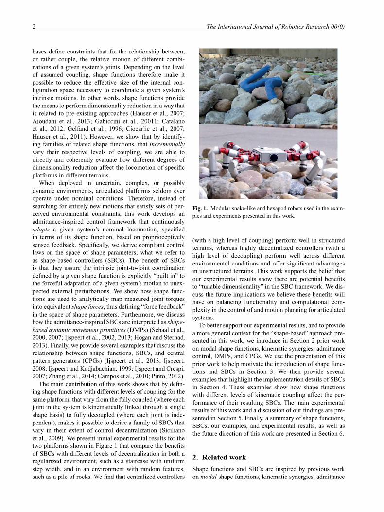
Fig. 1. Modular snake-like and hexapod robots used in the exam-
ples and experiments presented in this work.
(with a high level of coupling) perform well in structured
terrains, whereas highly decentralized controllers (with a
high level of decoupling) perform well across different
environmental conditions and offer significant advantages
in unstructured terrains. This work supports the belief that
our experimental results show there are potential benefits
to “tunable dimensionality” in the SBC framework. We dis-
cuss the future implications we believe these benefits will
have on balancing functionality and computational com-
plexity in the control of and motion planning for articulated
systems.
To better support our experimental results, and to provide
a more general context for the “shape-based” approach pre-
sented in this work, we introduce in Section 2 prior work
on modal shape functions, kinematic synergies, admittance
control, DMPs, and CPGs. We use the presentation of this
prior work to help motivate the introduction of shape func-
tions and SBCs in Section 3. We then provide several
examples that highlight the implementation details of SBCs
in Section 4. These examples show how shape functions
with different levels of kinematic coupling affect the per-
formance of their resulting SBCs. The main experimental
results of this work and a discussion of our findings are pre-
sented in Section 5. Finally, a summary of shape functions,
SBCs, our examples, and experimental results, as well as
the future direction of this work are presented in Section 6.
2. Related work
Shape functions and SBCs are inspired by previous work
on modal shape functions, kinematic synergies, admittance
Travers et al. 3
control, and DMPs/CPGs. Each of these topics is briefly
introduced.
2.1. Modal shape functions
In Section 4, we present several examples of shape func-
tions for the snake-like robot shown in Figure 1. Each
of the snake-like robot shape functions are closely related
to the modal shape functions originally introduced by
Chirikjian and Burdick (1991, 1994). This previous work
originally focused on fixed-base continuum manipulators
modeled using three-dimensional backbone curves. A back-
bone curve reference set shape function was defined by
Chirikjian and Burdick (1994) in terms of four geomet-
ric parameters (that represent a Frenet–Serret frame, for
example (Do Carmo, 1976; Yamada and Hirose, 2006)),
Si( s, t) ∈ R, where i = {1, 2, 3, 4}, and s is a continuous
arc length. Furthermore, each Si( s, t) was defined such that
Si( s, t) =
N∑
j=1
aij( t)φij( s) (1)
where φij( s) represent modal functions, aij( t) are the
“modal participation factors,” and N is the total number
of modes. The modal representations in (1) were used
by Chirikjian and Burdick (1991, 1994) to help sim-
plify inverse kinematics problems for continuum manipu-
lators, effectively reducing the problem from an infinite-
dimensional optimization to an optimization over the finite
set of modal participation factors. A similar approach was
applied to derive the kinematics of a sidewinding snake
model by Burdick et al. (1993).
2.2. Kinematic synergies
Similar to previous approaches (Hauser et al., 2007, 2011;
Ajoudani et al., 2013; Gabiccini et al., 20011; Catalano
et al., 2012; Ciocarlie et al., 2007; Prattichizzo et al., 2006),
this work defines kinematics synergies in terms of functions
f that map scalar parameters σ ( t) ∈ R into N-dimensional
joint spaces, i.e. f : R → RN , where we assume the joint
angles θ ∈ RN .1 Furthermore, we assume each mapping
f is defined by a static basis vector β ∈ RN such that
f ( σ ( t) ) = σ ( t)β. Note that, depending on the definition of
β, changes in the synergy parameters σ ( t) can coordinate
the motion across potentially large collections of a system’s
joints. Thus, as previous work shows (Ciocarlie et al., 2007;
Ficuciello et al., 2011), low-dimensional collections of syn-
ergies, e.g. ( f1( σ1( t) ) , f2( σ2( t) ) , . . . , fM ( σM ( t) ) ), where
M < N , can be used to coordinate relatively articulate
motions for high-degree-of-freedom systems; in this sense,
kinematic synergies make it possible to perform dimen-
sionality reduction. Note that the concept of muscle syn-
ergies, which are related to kinematic synergies in the sense
that they provide evidence that low-dimensional activation
signals are used to coordinate complex, multi-degree-of-
freedom motions, have been studied quite extensively by the
neuroscience community; see Ting and Macpherson (2004)
and d’Avella et al. (2006) as well as the references therein.
Kinematic synergies are thus closely related to the modal
shape functions in (1), were the “motion” of the infinite-
dimensional backbone curves are coordinated using finite
collections of the modal participation factors aij( t). The
main differences between the two are that synergies are
directly defined for discrete joint spaces and easily extend
to general topologies, whereas previous work on modal
approaches focused on continuum systems with serial
topologies.
In addition, previous work by Prattichizzo et al. (2006),
Gabiccini et al. (20011), Wimboeck et al. (2011), and Cata-
lano et al. (2012) developed different aspects of force con-
trol methods defined directly in terms of postural synergies.
These previous works are related to the SBCs that are intro-
duced in Section 3.2. However, Prattichizzo et al. (2006),
Gabiccini et al. (20011), Wimboeck et al. (2011), and Cata-
lano et al. (2012) focused primarily on manipulation and the
explicit control of the extrinsic forces applied by a manip-
ulator on different objects. We show in the remainder of
this work that SBCs provide a fundamentally intrinsic force-
control approach that relies on very little information about
the environment and is designed specifically for locomotion
control in complex terrains.
Lastly, we note that an important topic in previous
work on both modal shape functions as well as synergies,
that is not directly addressed for shape functions in this
work, is how they are derived. For example, Gong et al.
(2014) extracted low-dimensional expressions from bio-
logical snake data using multi-dimensional singular-value
decomposition (SVD) to derive modal-shape bases for dif-
ferent locomotive behaviors. Godage et al. (2015) used a
Taylor expansion to analytically derive modal shape func-
tions for highly articulated manipulators. Santello et al.
(1998) also used SVD, but applied it to human grasping
data to numerically derive bases for a space of postural syn-
ergies. Hauser et al. (2007, 2011) used offline optimization
to derive whole-body synergies for a humanoid balancing
model. We make the claim that these previous works pro-
vide a roadmap of different methods that can be applied
to derive shape functions similar to those presented in this
work. A further discussion related to future methods for
automating the derivation of shape functions is presented
in Section 6.
2.3. Admittance control
The SBC framework presented in Section 3.2 is inspired
by, and in special cases directly related to, conventional
admittance control (Hogan, 1985; Lawrence, 1988). In
the broader context of force control methods, admittance
control is an indirect approach that takes in a force (or
torque) measurement and returns a desired position com-
mand. This desired command is then tracked by a low-level
position-based controller.
4 The International Journal of Robotics Research 00(0)
For example, consider a fixed-base manipulator with N
internal degrees of freedom, θ ∈ RN . The closed-loop
dynamics for the manipulator and its associated admittance
controller are, respectively,
θ + kd θ + kp( θ − θd) = τext (2)
Md( θd − θ0) +Bd( θd − θ0) +Kd( θd − θ0) = τext (3)
where kd and kp are positive gains, τext is the sensed joint
torque, θ0 is the nominal trajectory we wish the system to
track, Md is an effective mass, Bd an effective damping, and
Kd an effective spring constant (Lawrence, 1988; Ott et al.,
2010). Equation (2) represents the closed-loop dynamics
for the manipulator controlled by a joint-level PD control
law. The dynamics of the admittance controller in (3) adjust
the desired joint angle θd that appears in the manipulator’s
PD controller as a function of the sensed joint torque τext.
Equation (3) specifies that the dynamics of the desired joint
signal are equivalent to a forced spring–mass–damper.
2.4. DMPs
DMPs provide a general method for encoding goal directed
behaviors in the attractor dynamics of autonomous nonlin-
ear dynamical systems (Schaal et al., 2000, 2007; Ijspeert
et al., 2002, 2013; Hogan and Sternad, 2013). For example,
r = a (b( r0 − r) −r)+ F( t) +C( γ ) (4)
where r0 is a nominal set point, a and b control the response
of r, F( t) is a (nonlinear) forcing function, and C( γ ) is a
coupling term that depends on the parameters γ , defines a
DMP model (Ijspeert et al., 2013). Physically, r in (4) can be
used to represent different elements of a given system, such
as a set of joint angles or the pose of an end-effector frame.
In the case where F( t) = 0 and C( γ ) = 0, the dynamics
in (4) reduce to a simple linear point attractor and the value
of r will stabilize to the set point r0. In the more general
case, i.e. where F( t) 6= 0 and/or C( γ ) 6= 0, a variety of
complex behaviors can be encoded in the dynamics of r.
Note that allowing r = θd − θ0, C( γ ) = τext, and F( t) = 0,
the dynamics in (4) have the same form as the dynamics of
the admittance controller in (3). Admittance controllers are,
thus, interpreted as a special case of a DMP in this work.
2.4.1. CPGs. As noted by Ijspeert et al. (2013), CPGs are
equivalent to cyclic DMPs. In this work, we define CPGs to
be chains of N coupled oscillators where the dynamics of
each oscillator are modeled by
ρi = 2πνi +
N−1∑
j=1
wj sin( ρj − ρi − φij) (5)
ri = ai
(ai
4( Ri − ri) −ri
)
(6)
xi = ri sin( ρi) (7)
where (5) is referred to as the canonical system that is
integrated to determine the phase of oscillator i, ρj is the
phase of oscillator j, νi is an intrinsic frequency, and the
weighting terms wij and phase offset φij determine the cou-
pled relationship between oscillators i and j (Ijspeert and
Crespi, 2007). Equation (6) defines stabilizing dynamics for
the amplitude parameter r, where ai is a positive rate con-
stant, and Ri is the desired amplitude set point. The cyclic
function in (7) defines the output of each oscillator.2
3. Shape in compliant control
3.1. Shape functions
Shape functions provide the basis for specifying the kine-
matic coupling relationships between the motion of indi-
vidual degrees of freedom in the highly articulated systems
considered in this work. More specifically, a shape func-
tion h maps a collection of scalar shape parameters σ ( t) =
( σ1( t) , σ2( t) , . . . , σM ( t) ) ∈ 6 ⊂ RM , where 6 is the
shape parameter space that is defined by a time-varying set
of shape bases β( t) =(β1( t) ,β2( t) , . . . ,βM ( t) ) ∈ RN×M ,
into the N-dimensional joint space, θ ∈ RN , of a given
system, i.e. h : RM × R
+ → RN . We define that each
of the individual joints effected by a change in value of a
single shape parameter, through its associated shape basis,
are kinematically coupled in this work. Similar to modal
shape functions (Section 2.1) and kinematic synergies (Sec-
tion 2.2), this work, in part, considers shape functions that
couple the relative motion of collections of a system’s inter-
nal joints in such a way that the effective dimensionality
of the associated configuration space is reduced. In this
case, the dimension of the shape space is defined such that
M < N . However, the upper limit considered in this work
is M = N , which represents the case where there is no
inter-joint coupling.
Take as an example a system where θ ∈ R3,6 ⊂ R
2, and
we have the special case that the shape function is linear in
the shape parameters,
θ = h( σ ( t) , t) = σ1( t)β1( t) +σ2( t)β2( t) . (8)
Furthermore, we define the shape bases in (8) to be time
invariant; specifically β1 = [1, 0, −1] and β2 = [0, 1, 0]. In
this example, we would thus state that joints one and three
are kinematically coupled through changes in σ1( t) under
β1 and that joint two is independently controlled by σ2( t).
Note that shape functions are thus very closely related
to both kinematic synergies as well as to modal shape
functions. The primary differences are that shape func-
tions: (1) explicitly consider both point-to-point and cyclic
changes in the values of the parameters σi( t); (2) allow the
basis vectors βi( t) to be time varying; and (3) do not neces-
sarily assume that the shape functions are linear in the shape
parameters.
Travers et al. 5
3.2. SBC
Shape functions provide the basis for how a system’s inter-
nal degrees of freedom are coupled during nominal locomo-
tion. However, un-modeled features, uncertainty, etc., often
disturb nominal conditions and a controller is needed to
adapt the system’s behavior. SBCs are introduced in this
work to provide a generalizable framework for deriving
controllers that adapt the locomotive behaviors of artic-
ulated systems while explicitly preserving the intrinsic
coordination specified by different shape functions.
For example, consider the special case
θ = h( σ ( t) ) =
M∑
i=1
σi( t)βi = Jσ ( t) (9)
where the columns of J are time-invariant shape bases βi,
which are also assumed to be linearly independent, and
σ ( t) = [σ1( t) , σ2( t) , . . . , σM ( t) ]T. In this case it is pos-
sible to map a conventional admittance controller defined
in joint space into an equivalent expression defined in
shape-parameter space, 6. Specifically, computing the time
derivatives of the shape function h in (9), we find θ = J σ ,
and θ = J σ , which can be substituted into (3),
M ′d( σd − σ0) +B′
d( σd − σ0) +K ′d( σd − σ0) = C( τext) (10)
where M ′d = JTMdJ , B′
d = JTBdJ , K ′d = JTKdJ , C( τext) =
JTτext, σd is a desired shape parameterization, and σ0 a nom-
inal shape parameterization.3 The expression in (10), thus,
defines the dynamics of a shape-based admittance con-
troller with external forcing measured by the shape force
C( τext).
Similarly to (3), Equation (10) takes as input a set of
joint torques and produces a set of desired joint positions
as output. However, there is an intermediate step in which
the joint torques and dynamic response matrices in (3)
are explicitly mapped into the shape-parameter dynamics
(10). The shape-parameter dynamics are then numerically
integrated at each time step during the online implementa-
tion of the controller, producing an updated desired shape
parameterization σd . The desired joint angles (tracked by a
low-level position-based controller) are then determined by
using the shape function, i.e. θd = h( σd ,β).
Note that solving for σd by numerically integrating (10)
introduces the necessary condition that M ′d be invertible.
This is equivalent to the requirement that both Md be full
rank and that the shape bases be linearly independent.
While Md is user specified, and is thus assumed to be full
rank, several examples in Section 4 use shape functions
whose shape bases are not necessarily linearly independent.
In this case, we return to the observation in Section 2 that
an admittance controller defined in the joint space is a spe-
cial case of a DMP with torque-based feedback. We use this
observation to define that (10) is a special case of what we
refer to as a shape-based DMP.
Furthermore, leveraging the generality of DMPs,
Mσd σd + Bσd σd + Kσ
d ( σd − σ0) = C( τext) (11)
where Mσd , Bσd , and Kσ
d are assumed only to be positive def-
inite, with C( τext) = JTτext and J = ∂h/∂σ , also defines a
shape-based DMP.4 In this case, the desired shape param-
eters have a similar response to external forces as those in
(10), but (11) offers the benefit of relaxing the assumptions
on the shape bases. The shape-based DMP in (11) was used
as the basis for deriving SBCs in the examples presented
in Section 4 and experiments in Sections 5. Note that the
gains Mσd , Bσd , and Kσ
d are, in general, free parameters that
need to be defined. In each of the examples and experi-
ments presented in this work the gains were set such that
the associated shape dynamics (11) were critically damped.
4. Shape-based compliance in locomotion
We present the results from several examples where SBCs
were implemented on the two platforms shown in Figure 1.
The first platform was a snake-like robot and the second a
walking hexapod. Both robots were assembled using a com-
mon set of modular components (Rollinson et al., 2013,
2014b; Ford et al., 2014). Series-elastic actuators served
as the active degrees of freedom in each platform. Abso-
lute position encoders on each side of a torsional-elastic
spring, located just before the output of each actuator, made
it possible to measure the spring deflections and thus output
torques of each joint; these measurements were used in the
SBCs for both platforms.
The examples presented in this section are provided to
demonstrate the basic functionality of SBC as well as to
provide context for the practical difference between cen-
tralized versus decentralized kinematic coupling in com-
pliant, articulated control. In general, the exact values of
different parameters, such as the external forces applied or
relative magnitude of the gains (under the assumption that
the controller response remains critically damped), could be
varied quite significantly without changing the underlying
functionality of the controllers presented. More thorough
experimental results that evaluate the performance of SBCs
under different environmental conditions are presented in
Section 5.
In addition, each of the examples (except that shown in
Figure 8b) considers a static scene wherein the robots are
not locomoting; the examples are meant to clearly demon-
strate how SBCs with different levels of coupling react to
isolated external forces. To lend better insight into the per-
formance of the SBCs while the robots are moving through
different environments, using the shape functions presented
in this section, we note that the behavior of the controllers
are entirely independent of the phase of the underlying
shape functions. More specifically, the controllers function
by regulating the systems’ shape changes around nominal
shape patterns (specified by the shape functions). Whether
the nominal shape patterns are changing (i.e. when the
phase is varied) or are held fixed (as in the examples
presented in this section) the SBCs’ basic functionality
will remain exactly the same. Extension 1 presents several
6 The International Journal of Robotics Research 00(0)
examples that demonstrate the performance of SBCs while
the phases of different shape functions are continuously
varied.
4.1. Whole-body coupling
4.1.1. Snake-like robot. In each of the examples for the
snake-like robot presented in this work, the shape func-
tions are defined in terms of the planar serpenoid model
originally developed by Hirose (1987),
θ = A sin( ηs − ωt) (12)
where A is an amplitude parameter, η is the spatial fre-
quency that determines the number of waves formed by
the robot’s body, ω is the temporal frequency that deter-
mines how fast waves travel down the body, and s is the
arc length measured from the head of the robot. For the
discrete-bodied snake-like robot in Figure 1, s = {0, δs,
2 · δs, . . . , N · δs}, where δs is the link length and N = 18.
Note that the axes of rotation of adjacent joints are rotated
by 90◦ with respect to the centerline of the mechanism. As a
result, there are only N ′ = 9 co-planar joints in the system,
i.e. only half the system’s joints are controlled in each of the
planar examples presented in this section.
The serpenoid model in (12) can be rewritten in the form
of a shape function,
θ = h( σ ) = A( t) cos(ωt) sin( ηs) −A( t) sin(ωt) cos( ηs)
=
2∑
i
σi( t)βi (13)
where the shape parameters are σ1( t) = A( t) cos(ωt) and
σ2( t) = −A( t) sin(ωt), and the shape bases are β1 =
sin( ηs) and β2 = cos( ηs).5 We define that there is whole-
body or global coupling between each of the N ′ co-planar
joints under both β1 and β2 in (13); a change in either σ1( t)
or σ2( t) will effect a change in value of all N ′ joints (Travers
and Choset, 2015).
The dynamics of the SBC for the shape function in (13)
are expressed in the form (11) for this example,6 where
σ ( t) =( σ1( t) , σ2( t) ) and J = ∂h/∂σ = [β1,β2]. How-
ever, the fact that the shape parameters share both an
amplitude and frequency parameter allows us to reduce
the shape dynamics. Specifically, we use the fact that
σ = [cos(ωt) , − sin(ωt) ]TA( t) = JAA( t) to rewrite (11)
in terms of the dynamics associated with A( t) directly,
MAd Ad + BA
d Ad + KAd ( Ad − A0) = CA( τext) (14)
where MAd = (JA)T Mσ
d JA, BAd = ( JA)T Bσd JA + 2( JA)T Mσ
d
JA, KAd = ( JA)T Kσ
d JA + ( JA)T Bσd JA + ( JA)T Mσd JA, and
CA( τext) = JAJτext. Note that we assume Mσd is positive
definite and, thus, MAd is positive by definition, i.e. (14) can
always be solved for Ad .
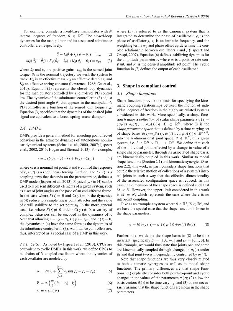
Figure 2 shows the results of implementing the SBC
defined by (14) on the snake-like robot. In this example
Fig. 2. Example of the whole-body coupled SBC implemented on
the snake-like robot. A single-amplitude parameter of the static
waveform shown is compliantly controlled in response to the
external forces applied.
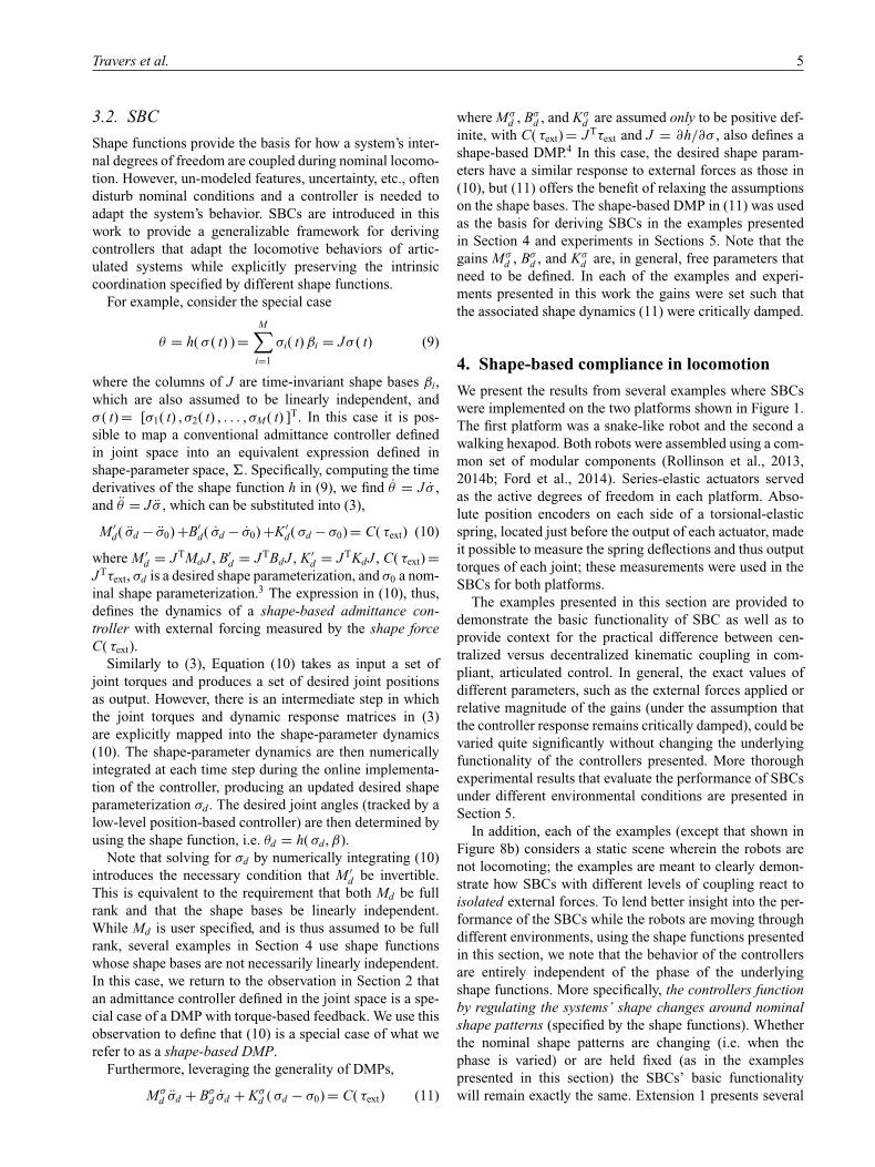
Fig. 3. Modular hexapod robot.
ω = 0, i.e. the wave on the robot’s body was station-
ary, A0 = 1, and Ad( 0) = A0. The plot on the left-hand
side of Figure 2 shows that at t = 0 no external force
was measured by the robot, i.e. the corresponding shape
force was approximately zero. At t = 1 an external force
was applied to the robot’s body, creating a negative shape
force and subsequently causing the value of Ad to decrease.
Note that due to the whole-body coupling defined by the
shape bases in (13), the amplitude simultaneously decreases
over the robot’s entire body. At t = 3.5 the external force
was removed, causing the shape force to return to approxi-
mately zero, and thus driving the desired amplitude param-
eter back to A0 = 1. Note that the controller implemented
in the example shown in Figure 2 is the static counterpart to
the “single-amplitude” SBC included in the experiments in
Section 5.
Note also that the dynamics in (14) define a reduced
shape-based DMP that bears a strong resemblance to the
oscillator amplitude dynamics in the CPG model in (6).
More specifically, rearranging (14) and defining a constant
Travers et al. 7
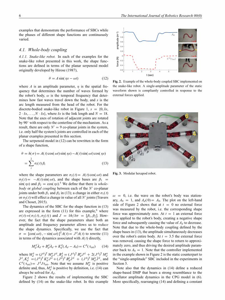
Fig. 4. Example of the whole-body coupled SBC implemented on
the hexapod robot. A single parameter controls the offset of each
leg in response to the external forces applied.
temporal frequency parameter ν,
ρ = 2πν
Ad =( MAd )−1 ( CA( τext) −BA
d Ad − KAd ( Ad − A0) )
θ = Ad sin( ηs − ρ)
provides an interpretation of the whole-body coupled SBC;
it defines a single oscillator whose time-varying amplitude
dynamics are a function of torque feedback (see (5)–(7)).
4.1.2. Hexapod robot. The shape functions used to define
SBCs for the hexapod robot shown in Figure 1 make the
assumption that, when the robot is walking, it continuously
executes an alternating tripod gait. More specifically, each
leg of the robot has three joints; a proximal joint, θ ip, that
rotates about a body-fixed yaw axis, and two distal joints,
θ id1 and θ i
d2, that rotate about body-fixed pitch axes (see Fig-
ure 3). The individual joint trajectories for leg i are defined
by
θ ip = Ai( t) +c1 cos(ω · t − φ) (15)
θ id1 = c2 sin(ω · t − φ) /( 1 + exp( −c3 sin(ω · t − φ) ) )
(16)
θ id2 = −c2 sin(ω · t − φ) /( 1 + exp( −c3 sin(ω · t − φ) ) )
(17)
where i ∈ {1, 2, . . . , 6}, c1, c2, and c3 are constants that
determine the stride length, maximum height of each foot
during flight, and shape of the foot trajectory (during flight),
respectively. The amplitude parameter A( t) in (15) controls
the offset position around which the proximal joint in each
leg oscillates. The trajectories of the two distal joints, (16)
and (17), have sigmoidal “activation windows” that lift the
feet with sinusoidal trajectories for one half of the gait cycle
and set the joint values equal to zero in the other half of the
cycle, i.e. during stance. The phase parameter φ is set to
zero for legs 1, 4, and 5 and is equal to π for legs 2, 3, and
6, i.e. the three legs in each support tripod are π radians out
of phase relative to the legs in the opposing tripod.
Shape functions for the hexapod are represented by θ =
h( σ ) =( θ1p , θ1
d1, θ1d2, . . . , θ6
p , θ6d1, θ6
d2) ∈ R18, i.e. the sequen-
tial list of the joint angles in each leg. We define the
shape parameters in terms of different combinations of
the proximal-joint offsets Ai( t) that appear in the trajecto-
ries (15) for each leg. More specifically, the shape functions
can be simplified to
θ = h( σ ,β, t) =
M∑
i
σi( t)βi + f ( t) (18)
where the function f ( t) represents the joint trajectories that
coordinate the alternating tripod gait under nominal con-
ditions, the shape parameters are σi( t) = Ai( t), and the
shape bases βi ∈ R18 contain zeros in the 12 rows that
correspond to the distal joints in the system; the number
of shape bases M and position of non-zero entries in the
six rows of the βi that correspond to the proximal joints
in θ (i.e. {β( 1) ,β( 4) , . . . ,β( 16) }) determine the kine-
matic coupling in the hexapod shape functions. For exam-
ple, in the case where M = 1 and we assume that β has six
non-zero entries, we define that the system is whole-body
coupled; changing the value of σ will effect the offset of
each leg.
Figure 4 shows the result of implementing the whole-
body coupled SBC on the hexapod robot while it was sus-
pended above the ground, the frequency ω of the alternating
tripod gait was set to zero (see (15)–(17)), and J in (11) was
defined by J = β. During the example, an external force
was first locally applied in the positive direction to leg 1.
Note that the offsets of all six legs were rotated in the posi-
tive direction about a body-fixed axis pointing vertically up
in response. At time t = 6 a force was applied to leg 6 in
the opposite direction, creating a negative shape force that
caused the offsets of all six proximal joints to rotate in the
negative direction with respect to the body-fixed frame.7
4.2. Decentralized coupling
This work assumes that SBCs with whole-body coupling
are centralized control methods in the sense that forces
applied locally to a robot’s body will affect global changes
in its shape. The experimental results that are presented
in Section 5 demonstrate that this type of global change
in shape works best in regularized environments. However,
in complex terrains, the global shape that is preserved by
centralized SBCs may not be compatible with the local
environmental features. More specifically, the body shapes
necessary to locally comply to irregular features in unstruc-
tured terrains may be outside the span of the shape bases
defined in the fully coupled shape functions. In this case,
this work supports the belief that a higher degree of decen-
tralization in the SBCs, in which fewer individual degrees
of freedom are kinematically coupled, may be necessary to
enable robots to locomote effectively.
8 The International Journal of Robotics Research 00(0)
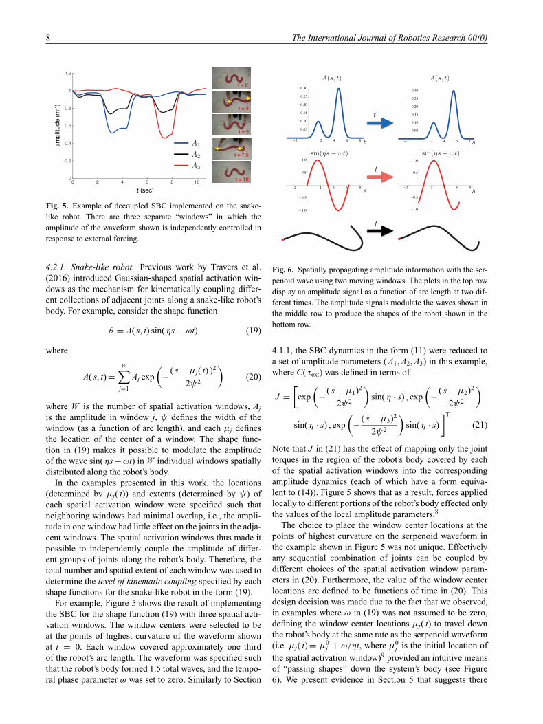
Fig. 5. Example of decoupled SBC implemented on the snake-
like robot. There are three separate “windows” in which the
amplitude of the waveform shown is independently controlled in
response to external forcing.
4.2.1. Snake-like robot. Previous work by Travers et al.
(2016) introduced Gaussian-shaped spatial activation win-
dows as the mechanism for kinematically coupling differ-
ent collections of adjacent joints along a snake-like robot’s
body. For example, consider the shape function
θ = A( s, t) sin( ηs − ωt) (19)
where
A( s, t) =
W∑
j=1
Aj exp
(
−( s − µj( t) )2
2ψ2
)
(20)
where W is the number of spatial activation windows, Aj
is the amplitude in window j, ψ defines the width of the
window (as a function of arc length), and each µj defines
the location of the center of a window. The shape func-
tion in (19) makes it possible to modulate the amplitude
of the wave sin( ηs −ωt) in W individual windows spatially
distributed along the robot’s body.
In the examples presented in this work, the locations
(determined by µj( t)) and extents (determined by ψ) of
each spatial activation window were specified such that
neighboring windows had minimal overlap, i.e., the ampli-
tude in one window had little effect on the joints in the adja-
cent windows. The spatial activation windows thus made it
possible to independently couple the amplitude of differ-
ent groups of joints along the robot’s body. Therefore, the
total number and spatial extent of each window was used to
determine the level of kinematic coupling specified by each
shape functions for the snake-like robot in the form (19).
For example, Figure 5 shows the result of implementing
the SBC for the shape function (19) with three spatial acti-
vation windows. The window centers were selected to be
at the points of highest curvature of the waveform shown
at t = 0. Each window covered approximately one third
of the robot’s arc length. The waveform was specified such
that the robot’s body formed 1.5 total waves, and the tempo-
ral phase parameter ω was set to zero. Similarly to Section
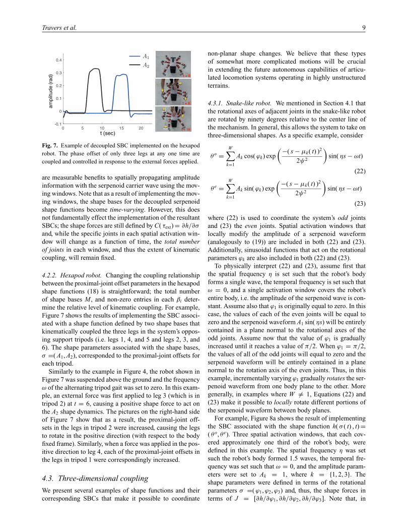
Fig. 6. Spatially propagating amplitude information with the ser-
penoid wave using two moving windows. The plots in the top row
display an amplitude signal as a function of arc length at two dif-
ferent times. The amplitude signals modulate the waves shown in
the middle row to produce the shapes of the robot shown in the
bottom row.
4.1.1, the SBC dynamics in the form (11) were reduced to
a set of amplitude parameters ( A1, A2, A3) in this example,
where C( τext) was defined in terms of
J =
[
exp
(
−( s − µ1)2
2ψ2
)
sin( η · s) , exp
(
−( s − µ2)2
2ψ2
)
sin( η · s) , exp
(
−( s − µ3)2
2ψ2
)
sin( η · s)
]T
(21)
Note that J in (21) has the effect of mapping only the joint
torques in the region of the robot’s body covered by each
of the spatial activation windows into the corresponding
amplitude dynamics (each of which have a form equiva-
lent to (14)). Figure 5 shows that as a result, forces applied
locally to different portions of the robot’s body effected only
the values of the local amplitude parameters.8
The choice to place the window center locations at the
points of highest curvature on the serpenoid waveform in
the example shown in Figure 5 was not unique. Effectively
any sequential combination of joints can be coupled by
different choices of the spatial activation window param-
eters in (20). Furthermore, the value of the window center
locations are defined to be functions of time in (20). This
design decision was made due to the fact that we observed,
in examples where ω in (19) was not assumed to be zero,
defining the window center locations µj( t) to travel down
the robot’s body at the same rate as the serpenoid waveform
(i.e. µj( t) = µ0j + ω/ηt, where µ0
j is the initial location of
the spatial activation window)9 provided an intuitive means
of “passing shapes” down the system’s body (see Figure
6). We present evidence in Section 5 that suggests there
Travers et al. 9
t (sec)
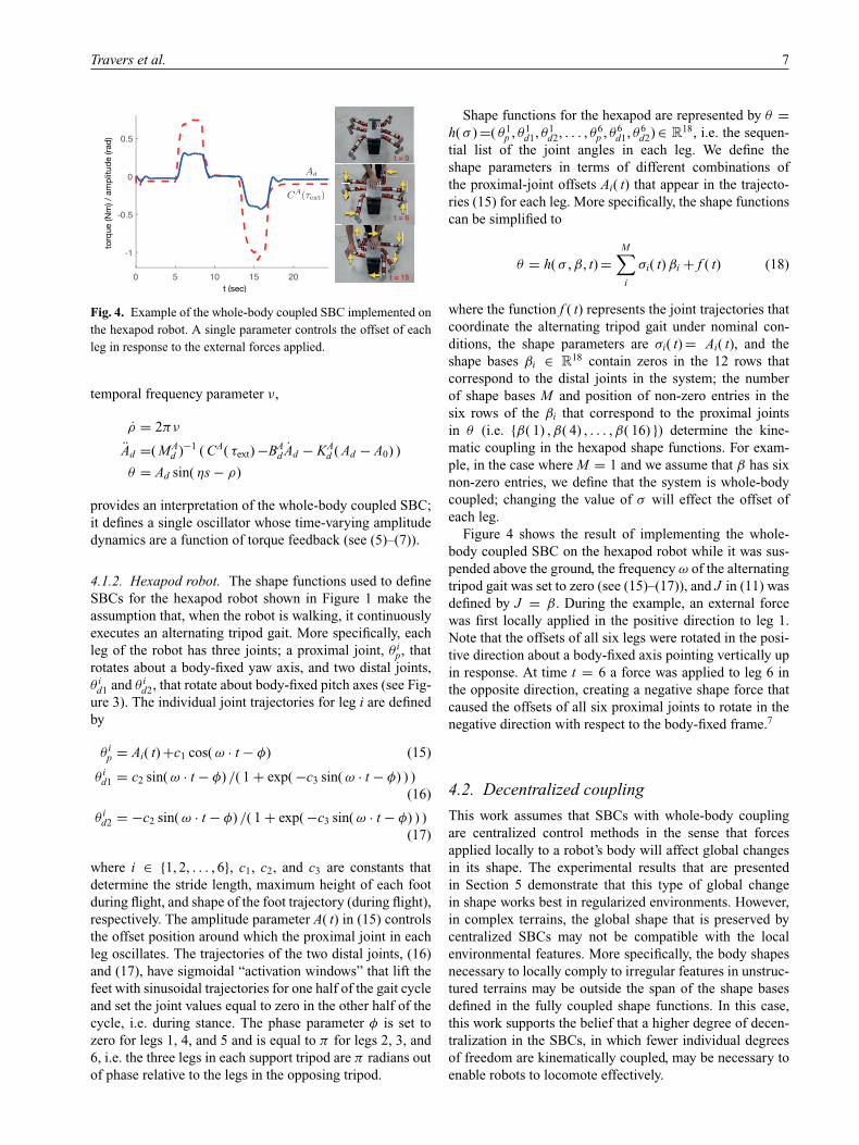
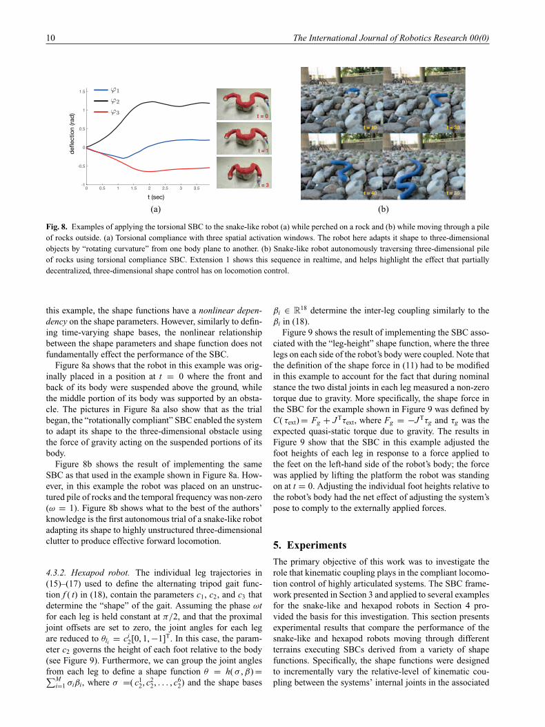
Fig. 7. Example of decoupled SBC implemented on the hexapod
robot. The phase offset of only three legs at any one time are
coupled and controlled in response to the external forces applied.
are measurable benefits to spatially propagating amplitude
information with the serpenoid carrier wave using the mov-
ing windows. Note that as a result of implementing the mov-
ing windows, the shape bases for the decoupled serpenoid
shape functions become time-varying. However, this does
not fundamentally effect the implementation of the resultant
SBCs; the shape forces are still defined by C( τext) = ∂h/∂σ
and, while the specific joints in each spatial activation win-
dow will change as a function of time, the total number
of joints in each window, and thus the extent of kinematic
coupling, will remain fixed.
4.2.2. Hexapod robot. Changing the coupling relationship
between the proximal-joint offset parameters in the hexapod
shape functions (18) is straightforward; the total number
of shape bases M , and non-zero entries in each βi deter-
mine the relative level of kinematic coupling. For example,
Figure 7 shows the results of implementing the SBC associ-
ated with a shape function defined by two shape bases that
kinematically coupled the three legs in the system’s oppos-
ing support tripods (i.e. legs 1, 4, and 5 and legs 2, 3, and
6). The shape parameters associated with the shape bases,
σ =( A1, A2), corresponded to the proximal-joint offsets for
each tripod.
Similarly to the example in Figure 4, the robot shown in
Figure 7 was suspended above the ground and the frequency
ω of the alternating tripod gait was set to zero. In this exam-
ple, an external force was first applied to leg 3 (which is in
tripod 2) at t = 6, causing a positive shape force to act on
the A2 shape dynamics. The pictures on the right-hand side
of Figure 7 show that as a result, the proximal-joint off-
sets in the legs in tripod 2 were increased, causing the legs
to rotate in the positive direction (with respect to the body
fixed frame). Similarly, when a force was applied in the pos-
itive direction to leg 4, each of the proximal-joint offsets in
the legs in tripod 1 were correspondingly increased.
4.3. Three-dimensional coupling
We present several examples of shape functions and their
corresponding SBCs that make it possible to coordinate
non-planar shape changes. We believe that these types
of somewhat more complicated motions will be crucial
in extending the future autonomous capabilities of articu-
lated locomotion systems operating in highly unstructured
terrains.
4.3.1. Snake-like robot. We mentioned in Section 4.1 that
the rotational axes of adjacent joints in the snake-like robot
are rotated by ninety degrees relative to the center line of
the mechanism. In general, this allows the system to take on
three-dimensional shapes. As a specific example, consider
θo =
W∑
k=1
Ak cos(ϕk) exp
(
−( s − µk( t) )2
2ψ2
)
sin( ηs − ωt)
(22)
θ e =
W∑
k=1
Ak sin(ϕk) exp
(
−( s − µk( t) )2
2ψ2
)
sin( ηs − ωt)
(23)
where (22) is used to coordinate the system’s odd joints
and (23) the even joints. Spatial activation windows that
locally modify the amplitude of a serpenoid waveform
(analogously to (19)) are included in both (22) and (23).
Additionally, sinusoidal functions that act on the rotational
parameters ϕk are also included in both (22) and (23).
To physically interpret (22) and (23), assume first that
the spatial frequency η is set such that the robot’s body
forms a single wave, the temporal frequency is set such that
ω = 0, and a single activation window covers the robot’s
entire body, i.e. the amplitude of the serpenoid wave is con-
stant. Assume also that ϕ1 is originally equal to zero. In this
case, the values of each of the even joints will be equal to
zero and the serpenoid waveform A1 sin( ηs) will be entirely
contained in a plane normal to the rotational axes of the
odd joints. Assume now that the value of ϕ1 is gradually
increased until it reaches a value of π/2. When ϕ1 = π/2,
the values of all of the odd joints will equal to zero and the
serpenoid waveform will be entirely contained in a plane
normal to the rotation axis of the even joints. Thus, in this
example, incrementally varying ϕ1 gradually rotates the ser-
penoid waveform from one body plane to the other. More
generally, in examples where W 6= 1, Equations (22) and
(23) make it possible to locally rotate different portions of
the serpenoid waveform between body planes.
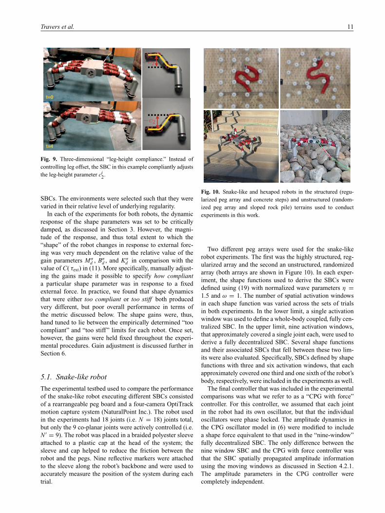
For example, Figure 8a shows the result of implementing
the SBC associated with the shape function h( σ ( t) , t) =
( θo, θ e). Three spatial activation windows, that each cov-
ered approximately one third of the robot’s body, were
defined in this example. The spatial frequency η was set
such the robot’s body formed 1.5 waves, the temporal fre-
quency was set such that ω = 0, and the amplitude param-
eters were set to Ak = 1, where k = {1, 2, 3}. The
shape parameters were defined in terms of the rotational
parameters σ =(ϕ1,ϕ2,ϕ3) and, thus, the shape forces in
terms of J = [∂h/∂ϕ1, ∂h/∂ϕ2, ∂h/∂ϕ3]. Note that, in
10 The International Journal of Robotics Research 00(0)
(a) (b)
Fig. 8. Examples of applying the torsional SBC to the snake-like robot (a) while perched on a rock and (b) while moving through a pile
of rocks outside. (a) Torsional compliance with three spatial activation windows. The robot here adapts it shape to three-dimensional
objects by “rotating curvature” from one body plane to another. (b) Snake-like robot autonomously traversing three-dimensional pile
of rocks using torsional compliance SBC. Extension 1 shows this sequence in realtime, and helps highlight the effect that partially
decentralized, three-dimensional shape control has on locomotion control.
this example, the shape functions have a nonlinear depen-
dency on the shape parameters. However, similarly to defin-
ing time-varying shape bases, the nonlinear relationship
between the shape parameters and shape function does not
fundamentally effect the performance of the SBC.
Figure 8a shows that the robot in this example was orig-
inally placed in a position at t = 0 where the front and
back of its body were suspended above the ground, while
the middle portion of its body was supported by an obsta-
cle. The pictures in Figure 8a also show that as the trial
began, the “rotationally compliant” SBC enabled the system
to adapt its shape to the three-dimensional obstacle using
the force of gravity acting on the suspended portions of its
body.
Figure 8b shows the result of implementing the same
SBC as that used in the example shown in Figure 8a. How-
ever, in this example the robot was placed on an unstruc-
tured pile of rocks and the temporal frequency was non-zero
(ω = 1). Figure 8b shows what to the best of the authors’
knowledge is the first autonomous trial of a snake-like robot
adapting its shape to highly unstructured three-dimensional
clutter to produce effective forward locomotion.
4.3.2. Hexapod robot. The individual leg trajectories in
(15)–(17) used to define the alternating tripod gait func-
tion f ( t) in (18), contain the parameters c1, c2, and c3 that
determine the “shape” of the gait. Assuming the phase ωt
for each leg is held constant at π/2, and that the proximal
joint offsets are set to zero, the joint angles for each leg
are reduced to θli = ci2[0, 1, −1]T. In this case, the param-
eter c2 governs the height of each foot relative to the body
(see Figure 9). Furthermore, we can group the joint angles
from each leg to define a shape function θ = h( σ ,β) =∑M
i=1 σiβi, where σ =( c12, c2
2, . . . , c62) and the shape bases
βi ∈ R18 determine the inter-leg coupling similarly to the
βi in (18).
Figure 9 shows the result of implementing the SBC asso-
ciated with the “leg-height” shape function, where the three
legs on each side of the robot’s body were coupled. Note that
the definition of the shape force in (11) had to be modified
in this example to account for the fact that during nominal
stance the two distal joints in each leg measured a non-zero
torque due to gravity. More specifically, the shape force in
the SBC for the example shown in Figure 9 was defined by
C( τext) = Fg + JTτext, where Fg = −JTτg and τg was the
expected quasi-static torque due to gravity. The results in
Figure 9 show that the SBC in this example adjusted the
foot heights of each leg in response to a force applied to
the feet on the left-hand side of the robot’s body; the force
was applied by lifting the platform the robot was standing
on at t = 0. Adjusting the individual foot heights relative to
the robot’s body had the net effect of adjusting the system’s
pose to comply to the externally applied forces.
5. Experiments
The primary objective of this work was to investigate the
role that kinematic coupling plays in the compliant locomo-
tion control of highly articulated systems. The SBC frame-
work presented in Section 3 and applied to several examples
for the snake-like and hexapod robots in Section 4 pro-
vided the basis for this investigation. This section presents
experimental results that compare the performance of the
snake-like and hexapod robots moving through different
terrains executing SBCs derived from a variety of shape
functions. Specifically, the shape functions were designed
to incrementally vary the relative-level of kinematic cou-
pling between the systems’ internal joints in the associated
Travers et al. 11
Fig. 9. Three-dimensional “leg-height compliance.” Instead of
controlling leg offset, the SBC in this example compliantly adjusts
the leg-height parameter ci2.
SBCs. The environments were selected such that they were
varied in their relative level of underlying regularity.
In each of the experiments for both robots, the dynamic
response of the shape parameters was set to be critically
damped, as discussed in Section 3. However, the magni-
tude of the response, and thus total extent to which the
“shape” of the robot changes in response to external forc-
ing was very much dependent on the relative value of the
gain parameters Mσd , Bσd , and Kσ
d in comparison with the
value of C( τext) in (11). More specifically, manually adjust-
ing the gains made it possible to specify how compliant
a particular shape parameter was in response to a fixed
external force. In practice, we found that shape dynamics
that were either too compliant or too stiff both produced
very different, but poor overall performance in terms of
the metric discussed below. The shape gains were, thus,
hand tuned to lie between the empirically determined “too
compliant” and “too stiff” limits for each robot. Once set,
however, the gains were held fixed throughout the experi-
mental procedures. Gain adjustment is discussed further in
Section 6.
5.1. Snake-like robot
The experimental testbed used to compare the performance
of the snake-like robot executing different SBCs consisted
of a rearrangeable peg board and a four-camera OptiTrack
motion capture system (NaturalPoint Inc.). The robot used
in the experiments had 18 joints (i.e. N = 18) joints total,
but only the 9 co-planar joints were actively controlled (i.e.
N ′ = 9). The robot was placed in a braided polyester sleeve
attached to a plastic cap at the head of the system; the
sleeve and cap helped to reduce the friction between the
robot and the pegs. Nine reflective markers were attached
to the sleeve along the robot’s backbone and were used to
accurately measure the position of the system during each
trial.
Fig. 10. Snake-like and hexapod robots in the structured (regu-
larized peg array and concrete steps) and unstructured (random-
ized peg array and sloped rock pile) terrains used to conduct
experiments in this work.
Two different peg arrays were used for the snake-like
robot experiments. The first was the highly structured, reg-
ularized array and the second an unstructured, randomized
array (both arrays are shown in Figure 10). In each exper-
iment, the shape functions used to derive the SBCs were
defined using (19) with normalized wave parameters η =
1.5 and ω = 1. The number of spatial activation windows
in each shape function was varied across the sets of trials
in both experiments. In the lower limit, a single activation
window was used to define a whole-body coupled, fully cen-
tralized SBC. In the upper limit, nine activation windows,
that approximately covered a single joint each, were used to
derive a fully decentralized SBC. Several shape functions
and their associated SBCs that fell between these two lim-
its were also evaluated. Specifically, SBCs defined by shape
functions with three and six activation windows, that each
approximately covered one third and one sixth of the robot’s
body, respectively, were included in the experiments as well.
The final controller that was included in the experimental
comparisons was what we refer to as a “CPG with force”
controller. For this controller, we assumed that each joint
in the robot had its own oscillator, but that the individual
oscillators were phase locked. The amplitude dynamics in
the CPG oscillator model in (6) were modified to include
a shape force equivalent to that used in the “nine-window”
fully decentralized SBC. The only difference between the
nine window SBC and the CPG with force controller was
that the SBC spatially propagated amplitude information
using the moving windows as discussed in Section 4.2.1.
The amplitude parameters in the CPG controller were
completely independent.
12 The International Journal of Robotics Research 00(0)
(a) (b)
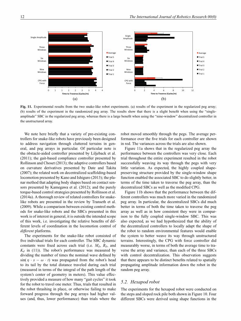
Fig. 11. Experimental results from the two snake-like robot experiments. (a) results of the experiment in the regularized peg array;
(b) results of the experiment in the randomized peg array. The results show that there is a slight benefit when using the “single-
amplitude” SBC in the regularized peg array, whereas there is a large benefit when using the “nine-window” decentralized controller in
the unstructured array.
We note here briefly that a variety of pre-existing con-
trollers for snake-like robots have previously been designed
to address navigation through cluttered terrains in gen-
eral, and peg arrays in particular. Of particular note is
the obstacle-aided controller presented by Liljeback et al.
(2011); the gait-based compliance controller presented by
Rollinson and Choset (2013); the adaptive controllers based
on curvature derivatives presented by Date and Takita
(2007); the related work on decentralized scaffolding-based
locomotion presented by Kano and Ishiguro (2013); the pla-
nar method that adapting body shapes based on contact sen-
sors presented by Kamegawa et al. (2012); and the purely
torque-based control strategies presented by Rollinson et al.
(2014a). A thorough review of related controllers for snake-
like robots are presented in the review by Transeth et al.
(2009). While a comparison between existing control meth-
ods for snake-like robots and the SBCs presented in this
work is of interest in general, it is outside the intended scope
of this work, i.e. investigating the relative benefits of dif-
ferent levels of coordination in the locomotion control of
different platforms.
The experiments for the snake-like robot consisted of
five individual trials for each controller. The SBC dynamic
constants were fixed across each trial (i.e. Md , Bd , and
Kd in (11)). The robot’s performance was measured by
dividing the number of times the nominal wave defined by
sin( η · s − ω · t) was propagated from the robot’s head
to its tail by the total distance traveled during each trial
(measured in terms of the integral of the path length of the
system’s center of geometry in meters). This value effec-
tively provided a measure of how many “gait cycles” it took
for the robot to travel one meter. Thus, trials that resulted in
the robot thrashing in place, or otherwise failing to make
forward progress through the peg arrays had higher val-
ues (and, thus, lower performance) than trials where the
robot moved smoothly through the pegs. The average per-
formance over the five trials for each controller are shown
in red. The variances across the trials are also shown.
Figure 11a shows that in the regularized peg array the
performance between the controllers was very close. Each
trial throughout the entire experiment resulted in the robot
successfully weaving its way through the pegs with very
little variation. As expected, the highly coupled shape-
preserving structure provided by the single-window shape
function enabled the associated SBC to do slightly better, in
terms of the time taken to traverse the peg array, than the
decentralized SBCs as well as the modified CPG.
Figure 11b shows that the performance between the dif-
ferent controllers was much more varied in the randomized
peg array. In particular, the decentralized SBCs did much
better in terms of both the time taken to traverse the peg
array as well as in how consistent they were in compar-
ison to the fully coupled single-window SBC. This was
also expected, as we had hypothesized that the ability of
the decentralized controllers to locally adapt the shape of
the robot to random environmental features would enable
the system to better weave its way through unstructured
terrains. Interestingly, the CPG with force controller did
measurably worse, in terms of both the average time to tra-
verse the array and variance, than each of the three SBCs
with control decentralization. This observation suggests
that there appears to be distinct benefits related to spatially
propagating amplitude information down the robot in the
random peg array.
5.2. Hexapod robot
The experiments for the hexapod robot were conducted on
the steps and sloped rock pile both shown in Figure 10. Four
different SBCs were derived using shape functions in the
Travers et al. 13
(a) (b)
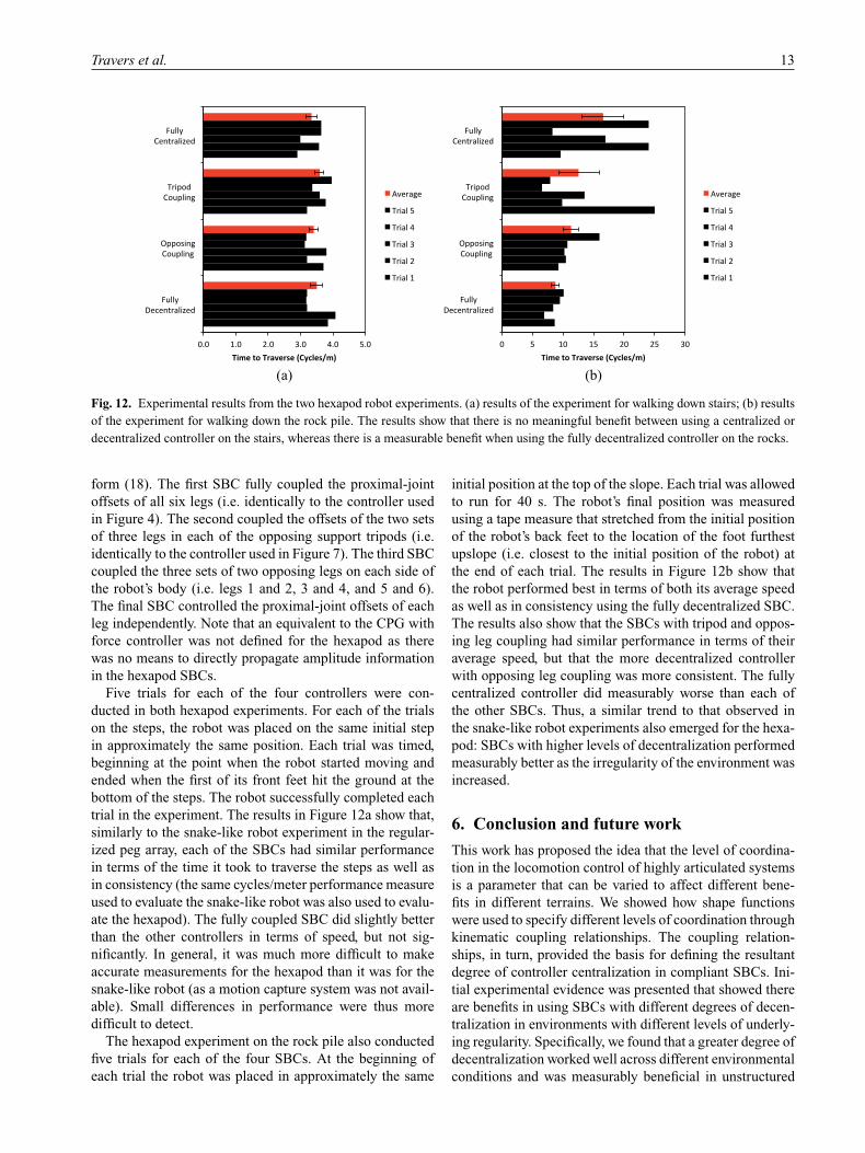
Fig. 12. Experimental results from the two hexapod robot experiments. (a) results of the experiment for walking down stairs; (b) results
of the experiment for walking down the rock pile. The results show that there is no meaningful benefit between using a centralized or
decentralized controller on the stairs, whereas there is a measurable benefit when using the fully decentralized controller on the rocks.
form (18). The first SBC fully coupled the proximal-joint
offsets of all six legs (i.e. identically to the controller used
in Figure 4). The second coupled the offsets of the two sets
of three legs in each of the opposing support tripods (i.e.
identically to the controller used in Figure 7). The third SBC
coupled the three sets of two opposing legs on each side of
the robot’s body (i.e. legs 1 and 2, 3 and 4, and 5 and 6).
The final SBC controlled the proximal-joint offsets of each
leg independently. Note that an equivalent to the CPG with
force controller was not defined for the hexapod as there
was no means to directly propagate amplitude information
in the hexapod SBCs.
Five trials for each of the four controllers were con-
ducted in both hexapod experiments. For each of the trials
on the steps, the robot was placed on the same initial step
in approximately the same position. Each trial was timed,
beginning at the point when the robot started moving and
ended when the first of its front feet hit the ground at the
bottom of the steps. The robot successfully completed each
trial in the experiment. The results in Figure 12a show that,
similarly to the snake-like robot experiment in the regular-
ized peg array, each of the SBCs had similar performance
in terms of the time it took to traverse the steps as well as
in consistency (the same cycles/meter performance measure
used to evaluate the snake-like robot was also used to evalu-
ate the hexapod). The fully coupled SBC did slightly better
than the other controllers in terms of speed, but not sig-
nificantly. In general, it was much more difficult to make
accurate measurements for the hexapod than it was for the
snake-like robot (as a motion capture system was not avail-
able). Small differences in performance were thus more
difficult to detect.
The hexapod experiment on the rock pile also conducted
five trials for each of the four SBCs. At the beginning of
each trial the robot was placed in approximately the same
initial position at the top of the slope. Each trial was allowed
to run for 40 s. The robot’s final position was measured
using a tape measure that stretched from the initial position
of the robot’s back feet to the location of the foot furthest
upslope (i.e. closest to the initial position of the robot) at
the end of each trial. The results in Figure 12b show that
the robot performed best in terms of both its average speed
as well as in consistency using the fully decentralized SBC.
The results also show that the SBCs with tripod and oppos-
ing leg coupling had similar performance in terms of their
average speed, but that the more decentralized controller
with opposing leg coupling was more consistent. The fully
centralized controller did measurably worse than each of
the other SBCs. Thus, a similar trend to that observed in
the snake-like robot experiments also emerged for the hexa-
pod: SBCs with higher levels of decentralization performed
measurably better as the irregularity of the environment was
increased.
6. Conclusion and future work
This work has proposed the idea that the level of coordina-
tion in the locomotion control of highly articulated systems
is a parameter that can be varied to affect different bene-
fits in different terrains. We showed how shape functions
were used to specify different levels of coordination through
kinematic coupling relationships. The coupling relation-
ships, in turn, provided the basis for defining the resultant
degree of controller centralization in compliant SBCs. Ini-
tial experimental evidence was presented that showed there
are benefits in using SBCs with different degrees of decen-
tralization in environments with different levels of underly-
ing regularity. Specifically, we found that a greater degree of
decentralization worked well across different environmental
conditions and was measurably beneficial in unstructured
14 The International Journal of Robotics Research 00(0)
terrains, whereas centralized SBCs offered slight perfor-
mance benefits in structured terrains. Two separate plat-
forms were employed in this work to support the generality
of our approach and results.
There are, however, several components related to shape
functions and SBCs that were not addressed in this work,
but that are the focus of ongoing and future work. The
first, as discussed in Section 2.2, addresses how shape func-
tions are derived. In each of the examples presented in this
work, the shape functions were highly system-specific and
user-defined. A natural question with respect to the broader
applicability of the shape-based framework is thus whether
or not the derivation of shape functions can be automated?
As discussed in Section 3.2, once a suitable shape func-
tion is defined, the process for deriving a controller that
acts directly on the shape parameters is relatively straight-
forward. Deriving shape functions is thus a necessary con-
dition for making the SBC framework, in its current form,
available to arbitrary robot architectures. In our future work,
we thus plan to derive shape functions for arbitrary systems
using a data-driven approach that is similar in concept to
that in Hauser et al. (2007, 2011). However, our planned
approach will focus on a broad simulation-based frame-
work where different platforms and a variety of environ-
mental conditions will be used to generate large amounts of
motion data. The data will be segmented into similar motion
patterns and assessed for quality. A combination of linear
and nonlinear dimensionality reduction techniques will then
be applied to the resulting data to derive, where possible,
low-dimensional representations of families of associated
motions. Our objective is to use the resulting expressions to
define different classes of shape functions.
This work additionally made the assumption that each of
the environments the robots’ were deployed in during test-
ing and experimentation were homogenous in the sense that
they were either structured or unstructured, but not a combi-
nation thereof. For the purpose of evaluating how the level
of coupling affected performance in different conditions,
the homogenous terrains were sufficient. However, in the
future we want to autonomously deploy highly articulated
systems in complex environments that contain a large vari-
ety of different terrains with varied underlying structure.
Based on the experimental observations made in this work,
it would thus be ideal to incorporate a higher-level planning
algorithm that actively manages the selection of different
shape functions, and their associated SBCs, based on a per-
ceived measure of environmental regularity. Several issues
will need to be addressed when developing such an algo-
rithm in future work, including how to define a “measure
of environmental regularity,” how to effectively transition
between different controllers/gaits, as well as the inher-
ent tradeoffs in terms of functionality versus computational
complexity.
More specifically, in the context of computational
complexity, decentralized controllers appear to provide
locomotive benefits across a broad range of environmental
conditions and, thus, appear to provide a better, or perhaps
more general approach in the experiments considered in this
work. However, this work also assumes that the nominal
parameters, σ0, around which each of the SBCs regulate are
given and that the gain matrices, Mσd , Bσd , and Kσ
d , that deter-
mine the compliance of controllers are operator defined and
are held fixed. In general, it would be ideal if a higher-level
planner could automatically determine these parameters at
runtime based on local information about the environment
and task specification (e.g. search an area, reach a goal
quickly, etc.). Automatically deriving the values of these
parameters during operation would make it possible to bet-
ter control behavioral-level tasks such as determining an
optimal forward speed, turning radius, etc. The decentral-
ized controllers inherently incorporate more parameters,
meaning that the planning search space would be higher
dimensional and, thus, more computationally costly. Thus,
by selecting between shape functions that vary in their
respective levels of coupling and, thus, in the dimension of
their underlying shape parameter spaces, the shape-based
approach will provide a potentially intuitive method for
implementing a planner with adaptive dimensionality that
is similar in concept to those in Gochev et al. (2011, 2012,
2013) in terms of striking a balance between functionality
and computational complexity.
Finally, even with an algorithm that selects between
shape functions that have different levels of kinematic cou-
pling, there was a limiting and an implicit assumption made
in this work that the spatial and temporal phases of the
underlying gait patterns, represented by the different shape
functions, were fixed. More specifically, each of the SBCs
presented in this work controlled only the relative ampli-
tudes of given motions. The controllers could thus scale
up or scale down a nominal motion, but could not actively
modify the underlying phasing between the different inter-
nal degrees of freedom in the robot (e.g. the hexapod robot’s
legs were constrained to execute a fixed alternating tripod
gait). We partially address this in our current work (Whit-
man et al., 2016), where we have started to explore how
coordination can be incorporated in controllers that com-
pliantly control both phase (spatial as well as temporal) as
well as amplitude. In our future work, we will look to more
explicitly combine the concepts of shape-based coordina-
tion and compliant SBCs with those related to the dynamic
phase coupling between oscillators typically identified in
CPG models.
Funding
The author(s) disclosed receipt of the following financial support
for the research, authorship, and/or publication of this article: This
work was supported in part by the Robotics Consortium of the U.S
Army Research Laboratory under the Collaborative Technology
Alliance Program and by the National Science Foundation under
Grant No. IIS-1724000.
Travers et al. 15
Notes
1. Note that there is a difference in terminology with respect to
the definition of a synergy in previous work. In particular, the
parameters σ ( t) are in some cases defined to be synergies.
2. The expression in (7) is slightly modified relative to the oscil-
lator output in Ijspeert and Crespi (2007). However, this modi-
fication does not change the salient features of the overall CPG
model.
3. We assume that shape functions in the form (9) are defined for
both the desired joint angles θd and nominal joint angles θ0 in
(3). We make this assumption throughout this work.
4. We assume the nominal shape parameterization σ0 is constant
in (11).
5. The shape function in (13) is equivalent to the modal shape
function in (1).
6. Although β1 and β2 are linearly independent, we use the more
general formulation of the shape-based DMP in (11) in this
example
7. If the robot were standing on the ground in this example and a
torque was applied about the vertical body axis, the whole-
body coupled SBC would cause the robot’s body to rotate
relative to the static positions of its stance feet. In examples
where the robot is walking, i.e. ω 6= 0, applying a torque
about the vertical body axis will cause the SBC to compliantly
change the robot’s heading.
8. The example in Figure 5 is included in this section because
it demonstrates the static response of the “three windows”
SBC included in the experiments presented in Section 5. The
reader is referred to the work of Rollinson and Choset (2013)
for a more direct demonstration of the practical benefits of
decentralized shape control wherein a snake-like robot exe-
cuting a controller that is similar in concept to a decentralized
SBC is shown successfully climbing the outside of a pipe with
varying diameter.
9. Note that this definition of µj( t) would require an infinite
number of windows to track the serpenoid waveform for all
time. We present a “recirculation condition” in the definition
of µj( t) in (Travers et al., 2016) that addresses this issue.
Supplemental Material
Supplementary video for this article is available online.
References
Ajoudani A, Godfrey S, Catalano M, Grioli G, Tsagarakis N and
Bicchi A (2013) Teleimpedance control of a synergy-driven
anthropomorphic hand. In: IEEE International Conference on
Intelligent Robots and Systems.
Alexandrov A, Frolov A and Massion J (1998) Axial syner-
gies during human upper trunk bending. Experimental Brain
Research 118(2): 210–220.
Burdick J, Radford J and Chirikjian G (1993) A “sidewind-
ing" locomotion gait for hyper-redundant robots. In: IEEE
Conference on Robotics and Automation.
Campos R, Matos V and Santos C (2010) Hexapod locomotion: a
nonlinear dynamical systems approach. In: Annual Conference
of the IEEE Industrial Electronics Society.
Catalano M, Grioli G, Serio A, Farnioli E, Piazza C and Bicchi
A (2012) Adaptive synergies for a humanoid robot hand. In:
IEEE Conference on Humanoid Robots.
Chirikjian G and Burdick J (1991) Parallel formulation of the
inverse kinematics of modular hyper-redundant manipulators.
In: Proceedings IEEE International Conference on Robotics
and Automation.
Chirikjian G and Burdick J (1994) A modal approach to
hyper-redundant manipulator kinematics. IEEE Transactions
on Robotics and Automation 10(3): 343–354.
Ciocarlie M, Goldfeder C and Allen P (2007) Dimensionality
reduction for hand-independent dexterous robotic grasping.
In: IEEE International Conference on Intelligent Robots and
Systems.
Date H and Takita Y (2007) Adaptive locomotion of a snake like
robot based on curvature derivatives. In: IEEE/RSJ Interna-
tional Conference on Intelligent Robots and Systems.
d’Avella A, Portone A, Fernandez L and Lacquaniti F (2006)
Control of fast-reaching movements by muscle synergy com-
binations. Journal of Neuroscience 30(26): 7791–7810.
Do Carmo M (1976) Differential Geometry of Curves and Sur-
faces. Enlewood Cliffs, NJ: Prentice-Hall.
Ficuciello F, Palli G, Melchiorri C and Siciliano B (2011) Exper-
imental evaluation of postural synergies during reach to grasp
with the UB hand IV. In: IEEE International Conference on
Intelligent Robots and Systems, pp. 1775–1780.
Ford S, Rollinson D, Willig A and Choset H (2014) Online calibra-
tion of a compact series elastic actuator. In: American Control
Conference (ACC).
Freitas S, Duarte M and Latash M (2006) Two kinematic synergies
in voluntary whole-body movements during standing. Journal
of Neuro-physiology 95(2): 636–645.
Gabiccini M, Bicchi A, Prattichizzo M and Malvezzi D (20011)
On the role of hand synergies in the optimal choice of grasping
forces. Autonomous Robots 31: 235–252.
Gelfand J, Lane S and Wilson W (1996) Synergy-based learning
of hybrid position/force control for redundant manipulators. In:
IEEE Conference on Robotics and Automation, April.
Gochev B K Cohen, Butzke J, Safonova A and Likhachev M
(2011) Path planning with adaptive dimensionality. In: Fourth
Annual Symposium on Combinatorial Search.
Gochev K, Safonova A and Likhachev M (2012) Planning with
adaptive dimensionality for mobile manipulation. In: IEEE
International Conference on Robotics and Automation, pp.
2944–2951.
Gochev K, Safonova A and Likhachev M (2013) Incremen-
tal planning with adaptive dimensionality. In: International
Conference on Automated Planning and Scheduling.
Godage I, Medrano-Cerda G, Branson D, Guglielmino E
and Caldwell D (2015) Modal kinematics for multisection
continuum arms. Bioinspiration and Biomimetics 10(3):
035002.
Gong C, Travers M, Kao H and Choset H (2014) Conditioned
basis array factorization: An approach to gait pattern extrac-
tion. In: Robotics: Science and Systems.
Hauser H, Neumann G and Ijspeert A (2007) Biologically inspired
kinematic synergies provide a new paradigm for balance
control of humanoid robots. In: IEEE Conference on Humanoid
Robots.
Hauser H, Neumann G, Ijspeert A and Maass W (2011) Biologi-
cally inspired kinematic synergies enable linear balance control
of a humanoid robot. Biological Cybernetics 104: 235–249.
Hirose S (1987) Biologically Inspired Robots (Snake-like Loco-
motor and Manipulator). Oxford: Oxford University Press.
16 The International Journal of Robotics Research 00(0)
Hogan N (1985) Impedance control: An approach to manipu-
lation, part I - Theory. ASME Journal of Dynamic Systems,
Measurement, and Control 107: 1–7.
Hogan N and Sternad D (2013) Dynamic primitives in the con-
trol of locomotion. Frontiers in Computational Neuroscience 7:
1–16.
Ijspeert A (2008) Central pattern generators for locomotion con-
trol in animals and robots: A review. Neural Networks 21:
642–653.
Ijspeert A and Crespi A (2007) Online trajectory generation in
an amphibious snake robot using a lamprey-like central pat-
tern generator model. In: IEEE International Conference on
Robotics and Automation.
Ijspeert A, Hoffmann H and Schaal S (2013) Dynamical move-
ment primitives: Learning attractor models for motor behav-
iors. Neural Computation 25: 328–373.
Ijspeert A and Kodjabachian J (1999) Evolution and development
of a central pattern generator for the swimming of a lamprey.
Artificial Life 5(3): 247–269.
Ijspeert A, Nakanishi J and Schaal S (2002) Movement imita-
tion with nonlinear dynamical systems in humanoid robots. In:
IEEE International Conference on Robotics and Automation.
Kamegawa T, Kuroki R, Travers M and Choset H (2012) Proposal
of Earli for the snake robot’s obstacle aided locomotion. In:
IEEE International Symposium on Safety, Security, and Rescue
Robotics.
Kano T and Ishiguro A (2013) Obstacles are beneficial to me!
Scaffold-based locomotion of a snake-like robot using decen-
tralized control. In: IEEE/RSJ International Conference on
Intelligent Robots and Systems.
Lawrence D (1988) Impedance control stability properties in com-
mon implementations. In: IEEE International Conference on
Robotics and Automation, pp. 1185–1190.
Liljeback P, Pettersen K, Stavdahl O and Gravdahl J (2011)
Experimental investigation of obstacle-aided locomotion with
a snake robot. IEEE Transactions on Robotics 27(4): 792–800.
Ott C, Mukherjee R and Nakamura Y (2010) Unified impedance
and admittance control. In: IEEE International Conference on
Robotics and Automation.
Pinto C (2012) Stability of quadruped robots’ trajectories sub-
jected to discrete perturbations. Nonlinear Dynamics 70: 2089–
2094.
Prattichizzo D, Malvezzi M and Bicchi A (2006) On motion and
force control of grasping hands with postural synergies. In:
Robotics: Science and Systems.
Rollinson D, Alwala K, Zevallos N and Choset H (2014a) Torque
control strategies for snake robots. In: IEEE/RSJ International
Conference on Intelligent Robots and Systems.
Rollinson D, Bilgen Y, Brown B, et al. (2014b) Design and archi-
tecture of a series elastic snake robot. In: IEEE/RSJ Interna-
tional Conference on Intelligent Robots and Systems.
Rollinson D and Choset H (2013) Gait-based compliant con-
trol for snake robots. In: IEEE International Conference on
Robotics and Automation.
Rollinson D, Ford S, Brown B and Choset H (2013) Design and
modeling of a series elastic element for snake robots. In: ASME
Dynamic Systems and Controls Conference.
Santello M, Flanders M and Soechting J (1998) Postural hand
synergies for tool use. Journal of Neuroscience 18(23): 10105–
10115.
Schaal S, Kotosaka S and Sternad D (2000) Nonlinear dynamical
systems as movement primitives. In: IEEE-RAS International
Conference on Humanoid Robots.
Schaal S, Mohajerian P and Ijspeert A (2007) Dynamics sys-
tems vs. optimal control—a unifying view. Progress in Brain
Research 165: 425–445.
Siciliano B, Sciavicco L, Villani L and Oriolo G (2009) Robotics:
Modelling, Planning, and Control. New York: Springer.
Ting L and Macpherson J (2004) A limited set of muscle syn-
ergies for force control during a postural task. Journal of
Neurophysiology (93): 609–613.
Transeth A, Pettersen K and Liljeback P (2009) A survey on snake
robot modeling and locomotion. Robotics 27: 999–1015.
Travers M and Choset H (2015) Shape-constrained whole-body
adaptivity. In: International Symposium on Safety, Security, and
Rescue Robotics.
Travers M, Whitman J, Schiebel P, Goldman D, and Choset H
(2016) Shape-based compliance in locomotion. In: Robotics:
Science and Systems.
Tricon V, Le Pellec-Muller A, Martin N, Mesure S, Azulay J
and Vernazza-Martin S (2007) Balance control and adapta-
tion of kinematic synergy in aging adults during forward trunk
bending. Neuroscience Letters 415(1): 81–86.
Whitman J, Ruscelli F, Travers M and Choset H (2016) Shape-
based compliant control with variable coordination centraliza-
tion on a snake robot. In: IEEE Conference on Decision and
Control.
Wimboeck T, Jan B and Hirzinger G (2011) Synergy-level
impedance control for a multifingered hand. In: IEEE Confer-
ence on Robotics and Automation.
Yamada H and Hirose S (2006) Study on the 3D shape of
active cord mechanism. In: IEEE International Conference on
Robotics and Automation.
Zhang J, Gao F, Han X, Chen X and Han X (2014) Trot gait design
and CPG method for a quadruped robot. Journal of Bionic
Engineering 11(1): 18–25.
Appendix: Index to multimedia extensions
Archives of IJRR multimedia extensions published prior
to 2014 can be found at http://www.ijrr.org, after 2014
all videos are available on the IJRR YouTube channel at
http://www.youtube.com/user/ijrrmultimedia
Table of Multimedia Extension
Extension Media type Description
1 Video Examples demonstrating the perfor-
mance of SBCs while the
phases of different shape functions
are continuously varied