Shadow Aware Object Detection and Vehicle...
101
Shadow Aware Object Detection and Vehicle Identification via License Plate Recognition Saameh Golzadeh Ebrahimi Submitted to the Institute of Graduate Studies and Research in partial fulfilment of the requirements for the Degree of Master of Science in Electrical and Electronic Engineering Eastern Mediterranean University September 2009 Gazimağusa, North Cyprus
Transcript of Shadow Aware Object Detection and Vehicle...

Shadow Aware Object Detection and Vehicle Identification via License Plate Recognition
Saameh Golzadeh Ebrahimi
Submitted to the Institute of Graduate Studies and Research
in partial fulfilment of the requirements for the Degree of
Master of Science in
Electrical and Electronic Engineering
Eastern Mediterranean University September 2009
Gazimağusa, North Cyprus

Approval of the Institute of Graduate Studies and Research ____________________________ Prof. Dr. Elvan Yılmaz Director (a) I certify that this thesis satisfies the requirements as a thesis for the degree of Master of Science in Electrical and Electronic Engineering. ______________________________________________ Assoc. Prof. Dr. Aykut Hocanın Chair, Department of Electrical and Electronic Engineering We certify that we have read this thesis and that in our opinion it is fully adequate in scope and quality as a thesis for the degree of Master of Science in Electrical and Electronic Engineering.
_____________________________________ Assoc. Prof. Dr. Erhan A. İnce Supervisor
Examining Committee ___________________________________________________________________________________________________________________ 1. Prof. Dr. N. Süha Bayındır ___________________________________________________________ 2. Assoc. Prof. Dr. Erhan A. İnce ___________________________________________________________
3. Prof. Dr. Runyi Yu ___________________________________________________________

iii
ABSTRACT
SHADOW AWARE OBJECT DETECTION AND VEHICLE
IDENTIFICATION VIA LICENSE PLATE RECOGNITION
This research proposes a comparative study between three shadow removal
algorithms and their application in license plate recognition. The idea is to monitor a
junction for red light violators and when one is detected to capture an image of the
vehicle along with its license plate details, which could be used to identify the driver.
Therefore, the focus of this research is on foreground segmentation, moving shadow
detection and elimination and license plate recognition procedures.
Moving cast shadows need careful consideration in order to develop accurate
object detection. Shadows may be misclassified as part of the foreground object and
this at times could cause merging of foreground objects, object shape distortion, and
even object losses (due to the shadow cast over another object). Therefore, the
removal of the shadows aids in more accurate detection of vehicle and hence, a
correct foreground for license plate recognition algorithms.
In this thesis, a background estimation / subtraction technique is applied to
segment the foreground and then three different shadow detection and removal
techniques are implemented and compared. First technique is based on the cast
shadow observations in luminance chrominance and gradient density making use of a
combined probability map called Shadow Confidence Score (SCS). Second method
exploits the HSV color space transform to converts pixel information from RGB color

iv
space to HSV domain. Third method is a hybrid color and texture-based approach
where chromacity conditions and texture similarities or dissimilarities of input and
background frames are considered in order to detect cast shadow parts. To evaluate
the performance of the various shadow removal algorithms ground-truth video
frames have been used as a quantitative scale. Finally, a correlation based LPR
algorithm was used to recognize the plate number of red light violators. First the
Radon transform was applied to estimate the skew angle of the detected foreground
objects and rotation angles were corrected. Then a color and edge based localization
for the license plate was carried out. After localization of the plate the individual
characters were segmented out using connected component analysis and the
characters to test were separated based on their Euler numbers. This was done
because Euler number filtering before the character recognition procedure is known
to improve the accuracy of the character recognition and also at the same time speeds
up the processing.
Keywords: Background estimation, foreground segmentation, shadow removal,
skew correction, license plate recognition,

v
ÖZET
GÖLGE BİLİNÇLİ NESNE TESBİTİ VE PLAKA TANIMA YOLUYLA
ARAÇ TANIMLAMA
Bu araştırma üç farklı gölge kaldırma yaklaşımı arasında karşılaştırmalı bir
çalışmayı ve bu çalışmanın görüntülü şehir trafik izlemede kırmızı ışık ihlali tesbiti
durumunda araç plakası tanımlama amacıyla bir kavşaktakta trafik kurallarını ihlal
eden araçların resimlerinin plakala detaylarıyla beraber yakalanmasının uygulamasını
sunmaktadır. Bu araştırmanın odağı önplan bölütleme, hareketli gölge tesbiti ve
giderilmesi ve plaka tanımlamadır.
Hareketli gölgelerin düşüm noktasının doğru nesne tebiti için dikkatle
gözönünde bulundurulması gerekmektedir. Gölgeler önplanın bir parçası olarak
yanlış sınıflandırılabilirler ve bu önplan nesnelerinin karışmasına, nesne şeklinin
bozukluğuna, ve hatta nesne kaybına (gölgenin birbaşka nesne üzerine düşmesi
sebebiyle) sebep olacaktır. Bu yüzden, gölgelerin kaldırılması araçların daha kesin
tesbit edilebilmesine ve dolayısıyla araç plaka tesbiti için daha uygun önplan
oluşturulmasına yardım etmektedir.
Bu tezde, önplanı bölütlemek amaçlı arkaplan tahmin/çıkarma tekniği
uygulanmıştır ve sonra üç farklı gölge tesbit ve kaldırma yaklaşımı uygulanmış ve
karşılaştırılmıştır. İlk yaklaşım, gölge güvenlirlik hesabı diye adlandırılan birleşik
olasılık haritası kullanılarak parlaklık/renklilik ve meyil yoğunluğundaki gölge
düşüm gözlemlerine dayanmaktadır. İkinci yöntem piksel bilgisini RGB renk
uzayından HSV alanına çevirmek için HSV renk boşluk transformunu kullanır.

vi
Üçüncü yöntem parlaklık durumlarının ve doku benzerliklerinin ya da girdi ve
arkaplan farklılıklarının gölge düşüm parçalarını tesbit etmek amacıyla göz önünde
bulundurulduğu parlaklık ve doku tabanlı yaklaşımdır. Çeşitli gölge kaldırma
algoritmalarının performansını ölçmek için referans video kareleri niceliksel ölçü
olarak kullanılmıştır. Son olarak, plaka tanımlama ve plaka numarası tanıma için bir
algoritma kullanılmıştır.
Anahtar Kelimeler: arkaplan kestirimi, önplan bölütleme, gölge kaldırma,
yamukluk açisi duzeltme, arac plakası tanime

vii
ACKNOWLEDGEMENTS
I would like to express my profound gratitude to Assoc. Prof. Dr. Erhan A.
İnce for his invaluable support, encouragement, supervision and useful suggestions
throughout this research work. His moral support and continuous guidance enabled
me to complete my work successfully. I am indebted to him more than he knows.
I gratefully acknowledge the head of the department Dr. Aykut Hocanın for
providing me an opportunity of studying in the department of Electrical and
Electronic Engineering as a research assistant.
I would like to extend my thanks to all of my instructors in the Electrical and
Electronic Engineering department who helped me so much for increasing my
knowledge.
I am as ever, especially indebted to my parents for their love and support
throughout my life. Finally, I also would like to express my appreciation to my
dearest Reza Nastaranpoor and my dear friends Majid Mokhtari, Nima seifnaraghi
and all other friends of mine who supported me all along.

viii
TABLE OF CONTENT
ABSTRACT ............................................................................................................... III
ÖZET .......................................................................................................................... V
ACKNOWLEDGEMENTS ...................................................................................... VII
TABLE OF CONTENT .......................................................................................... VIII
LIST OF FIGURES .................................................................................................. XII
LIST OF TABLES .................................................................................................. XIV
LIST OF ABBREVIATIONS / SYMBOLS .............................................................XV
CHAPTER 1 ................................................................................................................ 1
INTRODUCTION ....................................................................................................... 1
1.1 MOTIVATION ....................................................................................................... 5
1.2 RELATED WORKS ................................................................................................ 6
1.3 THESIS STRUCTURE ......................................................................................... 11
CHAPTER 2 .............................................................................................................. 12
BACKGROUND ESTIMATION .............................................................................. 12
2.1 INTRODUCTION .................................................................................................. 12
2.2 GROUP-BASED HISTOGRAM .............................................................................. 12
2.3 FOREGROUND SEGMENTATION .......................................................................... 17
CHAPTER 3 .............................................................................................................. 19
SHADOW REMOVAL ALGORITHMS .................................................................. 19

ix
3.1 SHADOW CONFIDENCE SCORE BASED SHADOW DETECTION .......................... 19
3.1.1 Introduction ............................................................................................... 19
3.1.2 Methodology .......................................................................................... 20
3.1.2.1 RGB to YCbCr Conversion ............................................................ 20
3.1.2.2 Observations about cast shadows ....................................................... 21
3.1.3 SCS Calculation ..................................................................................... 27
3.1.3.1 Luminance Score ........................................................................... 27
3.1.3.2 Chrominance Score ........................................................................ 28
3.1.3.3 Gradient Density Score .................................................................. 29
3.1.3.4 Combined SCS ............................................................................... 30
3.1.4 Moving Cast Shadow Detection and Elimination .................................. 31
3.2 SHADOW SUPPRESSION IN HSV COLOR SPACE ............................................... 32
3.2.1 Introduction ............................................................................................ 32
3.2.2 Methodology .......................................................................................... 33
3.2.2.1 RGB to HSV Conversion ............................................................... 33
3.2.2.2 Algorithm ....................................................................................... 34
3.3 HYBRID COLOR AND TEXTURE BASED SHADOW REMOVAL ............................ 37
3.3.1 Color Based Analysis ............................................................................. 38
3.3.1.1 Brightness Distortion ..................................................................... 38
3.3.1.2 Chromacity Distortion ................................................................... 39
3.3.2 Texture Based Analysis ......................................................................... 41
3.3.3 Morphological Reconstruction ............................................................... 41
3.4 EVALUATION................................................................................................... 43
3.4.1 Ground Truth Frames ............................................................................. 43
3.4.2 Recall & Precision ................................................................................. 44

x
3.4.2.1 Recall ............................................................................................. 44
3.4.2.2 Precision ......................................................................................... 45
3.4.3 Data Analysis ......................................................................................... 45
CHAPTER 4 .............................................................................................................. 46
LICENSE PLATE RECOGNITION ......................................................................... 46
4.1 INTRODUCTION .................................................................................................. 46
4.2 RED LIGHT TRACKING AND STOP LINE DETECTION .......................................... 47
4.3 ALGORITHM .................................................................................................... 49
4.3.1 License Plate Region Locating ............................................................. 50
4.3.1.1 Radon Transform ............................................................................... 50
4.3.1.2 Yellow Region Extraction .................................................................. 51
4.3.2 License Plate Character Segmentation ................................................... 55
4.3.3 License Plate Character Recognition ...................................................... 55
4.3.3.1 Euler Numbers and Characters .......................................................... 55
4.3.3.2 Digit Recognition ............................................................................... 57
4.4 EXPERIMENTAL EXAMPLES ............................................................................... 57
4.5 COMPARISONS WITH PREVIOUS DEPARTMENTAL WORKS AND THESIS RELATED
PUBLICATIONS ........................................................................................................ 59
CHAPTER 5 .............................................................................................................. 61
CONCLUSION AND FUTURE WORK .................................................................. 61
5.1 CONCLUSION ................................................................................................... 61
5.2 FUTURE WORK ................................................................................................ 63
APPENDICES ........................................................................................................... 64

xi
APPENDIX A: NOVEL TRAFFIC LIGHTS SIGNALING TECHNIQUE BASED ON LANE
OCCUPANCY RATES ................................................................................................ 65
APPENDIX B: TRAFFIC ANALYSIS OF AVENUES AND INTERSECTIONS BASED ON
VIDEO SURVEILLANCE FROM FIXED VIDEO CAMERAS ............................................ 70
REFERENCES .......................................................................................................... 74

xii
LIST OF FIGURES
Figure 1. 1: Cast shadow parts: "umbra" and "penumbra" .......................................... 4
Figure 2. 1: Statistic analysis of pixel intensity ......................................................... 17
Figure 2. 2: Foreground estimation using GBH technique ........................................ 18
Figure 3. 1: RGB to YCbCr Conversion ..................................................................... 21
Figure 3. 2: An outdoor background estimation and foreground segmentation ........ 22
Figure 3. 3: Luminance of masked input image and of the ....................................... 23
corresponding background ......................................................................................... 23
Figure 3. 4: Chrominance of masked input frame and of the .................................... 24
corresponding background image .............................................................................. 24
Figure 3. 5: Gradient Density of masked input frame and corresponding background
XXX image ........................................................................................................ 26
Figure 3. 6: Object and cast shadow separation using a convex hull [54] ................. 27
Figure 3. 7: Luminance Score of the masked input frame ......................................... 28
Figure 3. 8: Chrominance score of the masked input frame ...................................... 29
Figure 3. 9: Gradient Density Score .......................................................................... 30
Figure 3. 10: Total Shadow Confidence Score (SCS) ............................................... 31
Figure 3. 11: SCS shadow removal Algorithm .......................................................... 32
Figure 3. 12: Wheel and conical representation of HSV color model ....................... 33
Figure 3. 13: Shadow mask of a video frame at a junction in Famagusta ................. 36
Figure 3. 14: Shadow mask of highway-I video [56] ................................................ 36
Figure 3. 15: HSV color space result on shadow removal purpose ........................... 37
Figure 3. 16: Distortion measurements in the RGB Space ........................................ 38
Figure 3. 17: Brightness distortion of a traffic scene ................................................. 39

xiii
Figure 3. 18: Chromaticity distortion for a sample scene .......................................... 39
Table 3. 1: Shadow and highlight detection thresholds ............................................. 40
Figure 3. 19: Mask of texture based analysis ............................................................. 41
Figure 3. 20: Morphological AND result ................................................................... 42
Figure 3. 21: Detected foreground with shadows removed ....................................... 42
Figure 3. 22: Ground Truth video sequence for shadow removal evaluation, Highway
XXXX - I video sequence [56] .......................................................................... 44
Figure 4. 1:Examples of Mediterranean license plates .............................................. 46
Figure 4. 2: Samples for single and double line plates in TRNC............................... 47
Figure 4. 3: Traffic Lights .......................................................................................... 47
Figure 4. 4: Radon Transform .................................................................................... 51
Figure 4. 5: Yellow color pixel range in Hue component of HSI color space ........... 52
Figure 4. 6: License plate locating and extraction procedure .................................... 53
Figure 4. 7: Extracted License Plate Region .............................................................. 53
Figure 4. 8: Final version of binary license plate ....................................................... 54
Figure 4. 9: Vertical edge analysis for license plate detection .................................. 54
Figure 4. 10: Segmented characters of the license plate ............................................ 55
Figure 4. 11: Euler number example .......................................................................... 56
Figure 4. 12: License plate templates of characters and numbers ............................. 57

xiv
LIST OF TABLES
Table 1. 1 : Background Estimation Models ............................................................... 7
Table 1. 2 : Shadow Detector Approaches Taxonomy ................................................ 9
Table 2. 1 : Gaussian mean Error Estimation using conventional histogram and GBH
XXXX methods ................................................................................................. 15
Table 3. 1: Shadow and highlight detection thresholds ............................................. 40
Table 3. 2: Recall and Precision for different shadow removal algorithms ............... 45
Table 4. 1:License Plate Recognition Steps ............................................................... 49
Table 4. 2: Practical examples on LPR ...................................................................... 58

xv
LIST OF ABBREVIATIONS / SYMBOLS
YCbCr Luminance; Chroma: Blue; Chroma: Red
SCS Shadow Confidence Score
MFM Moving Foreground Mask
RGB Red, Green, Blue
GD Gradient Density
SAKBOT Statistical and Knowledge Based Object Tracker
HSV Hue, Saturation, Value
CMY Cyan, Magenta, Yellow
YUV Luminance, Bandwidth, Chrominance
BD Brightness Distortion
CD Chromacity (Color) Distortion
LPR License Plate Recognition
CCA Connected Component Analysis
WHR Width to Height Ratio
MATLAB MATrix LABoratory
GBH Group Based histogram
GMM Gaussian Mixture Model
TRNC Turkish Republic Of North Cyprus
ISS Intelligent Surveillance System
SNP Statistical Non-Parametric
SP Statistical Parameter
DM Deterministic Model-Based

xvi
DNM Deterministic Non-Model-Based
SVDD Support Vector Domain Description
FNN Feed-forward Neural Network
BRLS Block Recursive Least Square
MSE Mean Square Error
SVM Support Vector Machine
CCL Connected Component Labeling
SOM Self Organizing Map
HMM Hidden Markov Model
1
CHAPTER 1
INTRODUCTION
Real time segmentation of dynamic regions or objects in video or image
sequences is often referred to as “background subtraction” or “foreground
segmentation” and is a fundamental step in many computer vision applications.
Some examples include automated visual surveillance, traffic flow calculations,
object tracking, and detection of red light violations.
With new developments in computer and communications technologies the
need for improving Intelligent Surveillance Systems (ISS) technologies is becoming
more significant. The importance of visual traffic surveillance is its role in capturing
traffic data, detecting accidents and in safety management in general. It has been
demonstrated that vision based information processing will result in improved
operational efficiency.
The very first step in visual traffic processing is the segmentation of mobile
objects in image sequences. Based on the recorded image sequences a background
can be estimated and an old technique known as background subtraction is applied to
segment moving objects from each frame of the video. Background subtraction has
been utilized with various background estimation algorithms for different traffic
scenes. When the estimated background is fine then subtraction would lead to a good
estimate of the foreground mask [1]. However if the estimate is not good enough,

2
then the background subtraction method may result in a rough approximate of the
moving region. Furthermore with slow moving traffic it may even fail to provide a
result.
Illumination changes, shadow and inter-reflections, background fluctuations,
and crowded scenes are phenomena which cause problems for background
estimation. To handle some of these problems computationally expensive methods
are employed, where in practice such processing has to run in real-time. For instance,
most vision-based surveillance systems collect videos that are to be analyzed offline
at some later time. Background subtraction methods used in this manner, need also to
place a record of the date on the video so they can report on the results using this
date [3].
Real time methods are not able to handle properly one or more common
phenomena, such as global illumination changes, shadows, inter-reflections,
similarity of foreground object colors to that of the background, and non-static
backgrounds (i.e., tree branches and leaves waving in the wind). Different
background subtraction methods have been proposed over the last decades. The
simplest class of methods uses color or intensity as input and employs background
feature values (stillness) at each pixel to produce an independent, uni-modal
distribution. For example, Single-Gaussian (SG) model and group-based histogram
background estimation are such methods. [3]
When the current input frame is significantly different from the distribution
of expected background pixel vector, a foreground is detected on a per-pixel basis.
While dealing with color or intensity based background estimation algorithms
shadow points can also be detected as a part of the extracted foreground. In such

3
cases one needs to apply shadow detection and removal algorithms to have a more
correct FG representation.
Shadow is the name of the region produced by partial or entire occlusion of
direct light from a light source by an object. The procedure for identifying shadows
is divided into three processes: low level, medium level and high level [4]. The low
level process detects regions which are darker than their surroundings. Shadows are
among the dark regions. A middle level process detects features in dark regions such
as the penumbra, self-shadows and cast shadows. The object regions are adjacent to
dark regions. A high level process integrates these hypotheses and confirms the
consistency among the light directions estimated from them [4]. In general, a shadow
region is divided in to two parts: the self shadow and the cast shadow. The self-
shadow is the part of the object which is not illuminated by direct light. The cast
shadow is the area projected by the object in the way of direct light. Cast shadows in
the real world belong to illumination effects, because the light ray on its way from
the light source is affected by more than only one reflection on object surface.
Umbra is the part of a cast shadow where direct light is totally blocked by its
object. On the other hand, Penumbra is a part of a cast shadow where direct light is
partially blocked. These parts are depicted in Figure1.1. A point light source only
generates umbra in shadows. An “area” light source generates both penumbra and
umbra. When a penumbra is very small, it may not appear in an image due to
digitizing effects.

4
Figure 1. 1: Cast shadow parts: "umbra" and "penumbra"
In comparison to the penumbra area, umbra has lower light intensities
because umbra is receiving no light from the light source. These intensities increase
gradually from umbra to penumbra. The calculation of the luminance in a penumbra
is similar to that of an object surface, except that only a partial light source needs to
be considered [4]. The variations of the intensities in the penumbra area are not a
simple function of a light source and object. It is extremely difficult to achieve
theoretical formula of the intensities in a penumbra for an arbitrary object and an
arbitrary light.
As declared before, moving vehicles are often extracted with their associated
cast shadows after the application of background subtraction to traffic image
sequences. This phenomenon may lead to object losses, object shape distortion of
detected vehicle. In some other situations particularly when there are bunch of
vehicles near each other shadow of one vehicle may partially or completely be on
another vehicle and this results in misdetection of these two or a group of separate
vehicles as one big vehicle. Problems associated with occlusion would be created

5
afterwards. As a result the performance of the surveillance system would be affected
if the cast shadows are not detected and removed.
One of the applications of the shadow removal algorithms in traffic
surveillance system is controlling the traffic of vehicles by employing a License
Plate Recognition (LPR) system. An Intelligent Transportation System equipped with
LPR has many applications such as flexible and automatic highway toll
collection systems, analysis of city traffic during peak periods, enhanced vehicle
theft prevention, effective law enforcement, highest efficiency for border control
systems, building a comprehensive database of traffic movement, automation and
simplicity of airport and harbor logistics, security monitoring of roads and etc.
In general the LPR system consists of three major parts [30]: License Plate
detection, Character Segmentation and Character Recognition. A desired LPR system
has to work under different imaging conditions such as low contrast, blurring,
illumination and viewpoint changes. It is also supposed to perform properly in
complex scenes and bad weather conditions. In addition response time is another
restriction in real time applications such as license plate tracking. However, most of
the license plate recognition algorithms work under restricted conditions, such as
fixed illumination, limited vehicle speed, and stationary backgrounds.
1.1 Motivation
Management of present-day traffic in cities has become more important with
the gradual increase in traffic flow and traffic violations. In cities with heavy traffic
drivers tend to have a tendency to violate red lights and this behavior at times could
lead to accidents and even deaths. To deter the violators many state of the art
surveillance systems are being employed all over the world. The main aim of

6
research carried out in this thesis was to develop the essential blocks of a system that
could detect and identify red light violators in the city by the analysis of surveillance
video taken from a fixed video camera. In order to speed up license plate processing
and increase the accuracy of license plate detection it was decided that first the
foreground containing the red light violator(s) would be separated from the
background in the scene. To separate the foreground from the background in the
scene a background subtraction algorithm has to be implemented. In this study a
recently proposed state of the art BG modeling technique known as Group Based
Histogram (GBH) algorithm has been adopted.
1.2 Related Works
First step of this research is background estimation / subtraction. Background
estimation can be divided into two main categories: the predictive methods and the
non-predictive methods. The predictive methods arrange the sequence as a time
series and create a dynamical model at each pixel by considering the input frame,
past observations and magnitude of difference between the actual observation and the
predicted value. Non-predictive methods on the other hand, ignore the order of the
input observations and develop a probabilistic model for each pixel. In [40] Elhabian
states that background estimation algorithms can further be classified as non-
recursive and recursive models.
Alternatively, background estimation methods can be categorized in to
recursive modeling and non-recursive modeling techniques. A non-recursive
technique estimates the background based on a sliding-window approach and
recursive techniques update the background model using either a single or multiple
component (distribution) models at each pixel of the frame observed. Oliver et al.

7
[41] used an Eigen-background subtraction method which adaptively builds an Eigen
space that models the background method. A list of some non-recursive and some
recursive background modeling techniques has been given in Table 1.1. Non-
recursive modeling algorithms cover: frame differencing method in [57],[58],
average filtering approach [60], median filtering [61],[9], minimum–maximum
filtering method [62]. Recursive techniques include the approximated median
filtering method [63], single Gaussian technique [64], Kalman filtering method [65],
and Hidden Markov Models [66].
Table 1. 1 : Background Estimation Models
Over the past decades, several cast shadow detection methods have been
introduced and classified in region-based and pixel-based groups or as model-base
and shadow properties-base groups.
Many of these shadow detection algorithms are proposed for traffic
surveillance. It has been demonstrated in [5] that shadows can be extracted by
performing the difference between the current frame sk (at time k) and a reference

8
image s0 that can be the previous frame, as in [6], or a reference frame, typically
named “background model” as in [7][8][9].
Normally shadow detection algorithms are associated with techniques for
moving objects segmentation. Some of these techniques are based on the inter-frame
differencing [10],[11], background subtraction [12],[13], optical flow [14], statistical
point classification [15],[16] or feature matching and tracking [17],[18].
There are two important shadow and object visual features that cause
difficulties during shadow detection and removal. First, shadow points are detectable
as foreground points as they differ significantly from the background. Second,
shadow points have the same motion as the objects casting them. The goal of all
proposed algorithms is to prevent moving shadows being classified as moving
objects or parts of them, thus avoiding the merging of two or more objects into one
and improving the accuracy and performance of object localization.
The approaches in literature differ by means of how they distinguish between
foreground and shadow points. Most of these works locally exploit pixel appearance
change due to cast shadows [8],[4],[16],[6]. A possible approach is to compute the
ratio between the appearance of the pixel in the actual frame and the appearance in
the reference frame as in [6]. Most of the proposed shadow removal algorithms take
into account the model reported in [5], assume that camera and background are static
and light source is strong enough. To give explanation for their differences, as
demonstrated in Figure 1.2, four-class category of shadow detection algorithms are
presented according to the decision process: Statistical Non-Parametric (SNP),
Statistical Parametric (SP), Deterministic Model-based (DM) and Deterministic Non-
Model-based (DNM).

9
Table 1. 2 : Shadow Detector Approaches Taxonomy
Generally speaking shadow regions are detected and removed based on the
cast shadow observations of luminance, chrominance, and gradient density
considering geometry properties in YCbCr color space domain. A combined
probability map, called Shadow Confidence Score (SCS), of the region belonging to
the shadow is deduced and using the computed scores shadow region are separated.
The deterministic class [4],[6],[13] can be further subdivided. Sub-
classification can be based on whether the on/off decision can be supported by model
based knowledge or not. Choosing a model based approach as in [20], [6] achieves
undoubtedly the best results, but in most of the times, too complex and time
consuming compared to the non-model based [9][23]. Moreover, the number and the
complexity of the models increase rapidly if the aim is to deal with complex and
cluttered environments with different lighting conditions, object classes and
perspective views. It is also important to recognize the types of “features” utilized for
shadow detection. Basically, these features are extracted from three domains:
spectral, spatial and temporal. Approaches can exploit differently spectral features,
i.e. using gray level or color information. Some approaches improve results by using

10
spatial information working at a region level, instead of pixel level. Finally, some
methods exploit temporal redundancy to integrate and improve results.
In the statistical methods as in [15],[26],[67] the parameter selection is a
critical issue. Thus, we further divide the statistical approaches in parametric
methods such as [15],[22],[23],[27] and non-parametric methods. In Parametric
approach as in [15] an algorithm for segmentation of traffic scenes that distinguishes
moving objects from their moving cast shadows has been proposed. A fading
memory estimator calculates mean and variance of all three-color components for
each background pixel. Given the statistics for a background pixel, simple rules for
calculating its statistics when covered by a shadow are used. Then, MAP
classification decisions are made for each pixel.
Furthermore, Xu et al. [22] assumed that shadow often appears around the
foreground object and tried to detect shadows by extracting moving edges.
Morphological filters were used intensively. Toth et al. [23] proposed a shadow
detection algorithm based on color and shading information. This method changes
the color space from RGB space to LUV space.
A contour based method for cast vehicle shadow segmentation in a sequence
of traffic images taken from a stationary camera on top of a tall building is proposed
by Yan et al. [27]. Xiao et al. [28] proposed a method of moving shadow detection
based on edge information. Salvador et al. [29] introduced another method of shadow
removal based on the use of invariant color models to identify and to classify
shadows in digital images.
In literature, different approaches for applying license plate locating and
recognition have been proposed. The features that license plate locating employed
include shape, symmetry [43], height to width ration [44],[45], color [46],[45]

11
texture of grayness [47],[45], special frequency [31] and variance of intensity values
[49],[50].
License plate candidates determined by the plate localization stage are
examined to be involved in character separation and character recognition stages.
Different techniques used for character segmentation are projection [51],[52]
morphology [47],[48],[50] connected components [45] and blob coloring. Every
technique has its own disadvantages and advantages. The projection method assumes
the orientation of a license plate is known and the morphology method requires the
size of characters. In this research connected component technique is considered for
character separation since numbers and characters in English are composed of one
connected component region.
There is a large number of character recognition techniques reported. Some
of them are based on Neural Networks [31], [32], [34],[35], Generic Algorithm [33],
Edge Analysis [36],[37], Morphological Reconstruction [53], Markov Processes[38]
and Invariants Moment calculations[39].
1.3 Thesis Structure
The thesis is organized in the following manner: first chapter includes
introduction and a review on previous works. Chapter 2 introduces a Group-Based
Histogram algorithm as a background estimation / subtraction method to segment
moving foreground objects. In Chapter 3, three different shadow removal algorithms
are discussed and evaluated. An application based on foreground/background
separation, shadow detection and removal and license plate recognition processing is
introduced in Chapter 4. Finally, Chapter 5 provides conclusion and future work.

12
CHAPTER 2
BACKGROUND ESTIMATION
2.1 Introduction
Group-Based Histogram (GBH) technique is a recently suggested method to
generate a background model of each pixel from traffic image sequences. This
algorithm features improved robustness against transient stops of foreground objects
and sensed noise. Moreover, the method features low computational load, thus meets
the real-time requirements in many practical applications. The proposed method has
been used with vision-based traffic parameter estimation systems to segment moving
vehicles from image sequences.
2.2 Group-Based Histogram
The GBH algorithm constructs background model using the histogram of
intensities obtained from the current input frame and future frames at a specific
location (x,y). Unlike other histogram based methods, group based histogram is
forced to follow a Gaussian shaped trend to improve the quality of the estimated
background [19].
Although the histogram approach is robust to the transient stops of moving
foreground objects, the estimation is still less accurate than Gaussian Mixture Model

13
(GMM) in the case of non-static backgrounds (i.e. swaying grass, shaking leaves,
rain etc.). The proposed GBH method effectively exploits an average filter to
smoothen the frequency curve of ‘conventional’ histogram. From a smoothed
histogram a more accurate mean value and respectively standard deviation can be
estimated. One can easily and efficiently estimate the single Gaussian model
constructed by background intensities from image sequences during a fixed span of
time.
While doing background estimation based on histogram analysis, the
intensity with the maximum frequency in the histogram is treated as background,
because each intensity frequency in the histogram is proportional to its occurrence
probability. The background intensity can therefore be determined by analyzing the
intensity histogram. However, sensing variation and noise from image acquisition
devices or pixels having complex distributions may result in erroneous estimates.
This may cause a foreground object to have the maximum intensity frequency in the
histogram.
Since the maximum frequency of the histogram indicates the intensity of the
pixel belonging to the background model, there will not be any inclusion of slow
moving objects or transient stops in the detected foreground. However, the maximum
peak of the conventional histogram of each pixel will not necessarily locate the
intensity of background model at that specific pixel. In some cases this maximum
may not be unique so further processing may be needed to compensate the loss
which will affect the real time tracking.
In group based histogram each of the individual intensities is considered
along with its neighboring intensity levels and forms an accumulative frequency. The

14
frequency of coming intensity is summed up with its neighboring frequency to create
a Gaussian shape histogram.
The accumulation can be done by using an average filter of width 2w+1
where w stands for half width of the window. The output , of the average
filter at level l can be expressed as:
, , ; 0 1 (2.1)
where , is the count of the pixel having the intensity at the location
( , ) and is the number of intensity levels based on the number of bits in each
layer.
Maximum probability density , of a pixel at location ( , ) over the
recorded image frames can be computed through a simple division of the occurrence
for a pixel by, , the total frequency of the GBH.
, , (2.2)
If the width of the window is chosen to be less than a preset value, the
location of the maximum will be closer to the center of the Gaussian model than the
normal histograms. This is the result of the smoothening effect by the filter used.
Therefore the mean intensity of the background model will be:
µ , arg , (2.3)
For smaller window widths, the computational time will be less and the
accuracy of the background pixels estimates will vary for different window sizes and
standard deviations. To show how window width can be selected an example based
on 13 Gaussians generated by Gaussian random number generator can be given. The
mean for each Gaussian has been chosen as 205 and standard deviations varied

15
between 3 and 15. The percentage of errors while trying to estimate the background
pixels using the conventional histogram approach versus the GBH method are
depicted in Table 2.1. The window widths and the range of standard deviate values
(3-15) used in the comparisons have also been shown in the table.
Table 2. 1 : Error Estimation for the Gaussian mean using conventional histogram XX and GBH methods
The results prove the superiority of implementing GBH method to
conventional histograms. Considering the simulation results it can be concluded that
a greater window width will be needed for high-accuracy performance as the
standard deviation increases. According to the simulation results and error rate of
mean estimation within ± 2 %, the width, w, can be determined as follows [19]:
w =3 3 75 8 107 10 15 (2.4)
Where, represents the standard deviation of the original Gaussian.
As mentioned before, the mean intensity μ , can be computed by selecting
the maximum frequency of the smoothened histogram. When a new intensity l is
captured, the algorithm does not process all the possible intensities because there

16
would be very few neighboring pixels that fall in the selected window together with
the input intensity.
The steps of the procedure for estimating the mean of the distribution are as
follows. First, the current intensity l of the pixel is recorded. Second, the occurrence
frequency of that intensity and the intensities of neighbors from l-w to l+w is
incremented by one. Finally, the new maximum value is checked to see if it is greater
than the previously estimated mean value or not. If the condition is satisfied then
replacement of the former mean with the new one is made and then the algorithm
will return to the first step.
After computing the mean intensity of the Gaussian shaped histogram, the
variance could also be estimated using the following expression:
, 1∑ ,,, μ , ,,, (2.5)
where, is the maximum standard deviation of the Gaussian. Figure2.1 (b) demonstrates the histogram smoothing after the implementation
of average filtering window for a certain pixel in a traffic video sequence. From
Figure 2.1 (a) one can conclude that it would be possible to model the results with a
Gaussian distribution. However since several peaks with similar frequencies occur in
the histogram, selecting the mean is not straight forward. By applying the windowing
technique proposed in GBH the histogram will be smoothed and this multiple peaks
are eliminated.

17
(a) (b)
Figure 2. 1: Statistic analysis of pixel intensity
(a) Histogram (b) group-based histogram
To cope with the illumination changes of the environment, the histogram can
be re-built after every 15 minutes.
2.3 Foreground Segmentation
If the current pixel intensity under observation is to be accepted as
foreground, its distance from the mean of the distribution should not exceed three
times the standard deviation of the distribution. With this restriction a pixel at
location (u,v) on the image, can be assumed as a part of the foreground mask as
shown by equation 2.6 below:
, 1, | , , 3 , |0, (2.6)
where, µ(u,v) ,σ(u,v) represent mean and standard deviation of the background model
at location (u,v).
Figure 2.2 provides an example for background estimation by applying the
GBH approach on a video sequence at a junction. The segmented foreground objects

18
are vehicles and pedestrians with their corresponding cast shadows. On the
segmented foreground objects shadow removal algorithms are applied in order to get
vehicles without cast shadows.
(a) (b)
(c) (d)
Figure 2. 2: Foreground estimation using GBH technique
(a) An Input Frame of the Sequence (b) Estimated Background
(c) Moving Foreground Image Mask (d) Extracted Foreground
19
CHAPTER 3
SHADOW REMOVAL ALGORITHMS
As mentioned earlier, when the detected foreground mask contains shadows,
the calculated quantities such as location, dimension, speed, and number of vehicles
often include large errors. For instance, in a traffic scene with detached shadows
approximately the same size as the car, a vehicle’s location may be incorrectly
estimated as the shadow region. Long shadows could also connect two separate
vehicles as if they were a single object. Therefore, the performance of the overall
system may be seriously affected if the cast shadow is not detected and removed
efficiently. Below three different algorithms are introduced and compared against
each other for efficient and reliable detection of cast shadows.
3.1 Shadow Confidence Score Based Shadow Detection
3.1.1 Introduction
The robust method described in [54] has adopted YCbCr color space for
detecting cast shadows of moving vehicle in a monocular color traffic image
sequence. Firstly the background estimation/subtraction algorithm is used to generate
the foreground mask and then extracted blobs corresponding to binary mask
locations in the color image are converted to YCbCr.

20
The extracted foreground mask generally includes both the moving vehicles
and their cast shadows as a binary map. In [54] the mask is referred to as the Moving
Foreground Mask (MFM). From this MFM the Shadow Confidence Score (SCS) can
be calculated to indicate the likelihood of shadow according to the cast shadow
characteristics. The edge pixels of the input image within the MFM are classified into
object-edge pixels and non-object edge pixels. Then object-edge pixels are bounded
by a convex hull to generate a more accurate foreground mask of the moving
vehicles.
3.1.2 Methodology
3.1.2.1 RGB to YCbCr Conversion
YCbCr is an encoded nonlinear RGB signal. The Y-component is known as the
luminance value and is a weighted sum of the R, G, B components. “Cr” and “Cb” are
formed by subtracting the luminance component from red and blue components
respectively and multiplying the results by some weight factor. In this work the
YCbCr color space was chosen since it can separate luminance from color
components. This was a good idea since luminance values for shadow regions and
non-shadow regions would significantly vary from each other. The command used
for converting the color RGB image to YCbCr was RGB2YCBCR(.).
The Figure 3.1 and the equations given below show how one can transform
an RGB image into the YCbCr domain.

21
Figure 3. 1: RGB to YCbCr Conversion
(3.1) 0.7132 (3.2) 0.5647 (3.3)
3.1.2.2 Observations about cast shadows
In essence shadows can be classified as: the self -shadow and the cast
shadow. Self shadow is the part of the object that is not illuminated by direct light,
while cast shadow is the region projected by the object in the direction of direct light.
Even though changes in illumination and weather conditions could lead to cast
shadows that have different colors or tones, [54] states four generic features that are
generally true about cast shadow. In the sections that follow we try to explain these
four observations with the help of some examples. For identifying the correct
shadow pixels the SCS based processing would require the input frame, the estimated
background and the foreground binary mask as depicted in Figure 3.2 (a) –(c).

22
(a) (b)
(c)
Figure 3. 2: An outdoor background estimation and foreground segmentation
(a) Input frame, (b) Estimated Background, (c) Moving Foreground Mask
Figure 3.2 (a) shows an input frame containing a truck in an outdoor traffic
scene under bright sunlight with corresponding cast shadow. Figure 3.2 (b) represent
estimated background and Figure 3.2 (c) is the Moving Foreground Mask (MFM)
gained from difference of input frame and estimated background (a morphological
closing has been applied to join the discontinuities of the object). The small holes in
the foreground mask image are due to the similarities between the vehicle colors and
corresponding background that is subtracted from the input frame.

23
Observation1. The Luminance values of the cast shadow pixels in the input are
lower than those of the corresponding pixels in the background image.
As stated in [54], the cast shadow region is the darker region due to its lower
luminance values. The Figure 3.3 (a) demonstrates the luminance of the truck within
the mask region in the input frame and the luminance of the corresponding
background within the mask is depicted in Figure 3.3 (b). The subtraction between
the two masked regions is shown in Figure 3.3 (c). It’s obvious from the figures that
luminance of input image is most of the time lower than the background image in the
cast shadow region.
(a) (b)
(c)
Figure 3. 3: Luminance of masked input image and of the corresponding background
(a) Luminance of masked input frame, (b) Luminance of masked background
frame (c) Luminance difference between masked input and background frames

24
Observation2. The chrominance values of the cast shadow pixels are identical or
only slightly different from those of the corresponding pixels in the background
image.
The chrominance feature of foreground vehicle with its cast shadow based on
observation 2 is depicted in Figure 3.4. Luminance and chrominance components of
the images are separated in YCbCr color space. Cr and Cb components of masked
input frame and masked background frame are calculated separately. Absolute
difference between Cb component of masked input frame and background frame are
then taken (Figure 3.4 (a)). Similarly, the absolute difference of the Cr components is
depicted by Figure 3.4 (b). Finally, the sum of Cb and Cr absolute differences is
calculated and shown in Figure 3.4 (c). For typical sunlight, a decrease in
illumination will cause only a slight change in chrominance values of the shadow
pixels in both the masked input and the masked estimated background images.
(a) (b)
(c)
Figure 3. 4: Chrominance of masked input frame and of the corresponding background image
(a) Cb differences |CbI - CbB|, (b) Cr differences |CrI - CrB|, (c) Chrominance difference |CbI - CbB| + |CrI - CrB|

25
Observation3. The difference in gradient density values of the cast shadow pixels
and the corresponding background pixels is relatively low. The difference in gradient
density values between the vehicle and the corresponding background pixels is
relatively high.
Gradient Density (GD) is the average of gradient magnitudes over a local
area which can be computed using a spatial window as shown in the equation below:
, 12 1 | , , | (3.4)
Where, , , , are horizontal and vertical edge magnitude obtained using
‘Laplacian’ gradient operator for pixel (i,j) and (2ω +1) is the spatial window size.
According to Figure 3.5 (c) there is no significant gradient density difference
in the cast shadow region, but in the vehicle region the gradient density difference
between the masked input and background images varies considerably. Therefore,
one can assume that the majority of vehicle region pixels have large gradient density
differences.

26
(a) (b)
(c)
Figure 3. 5: Gradient Density of masked input frame and of the corresponding background image
(a) gradient density of the mask input, (b) gradient density of masked background frame, (c) gradient density difference
Observation4. The vehicle can be bounded approximately by means of a convex
mask. The cast shadow is an extension of the object mask.
The cast shadow can be separated from the foreground object based on the
shadow confidence scores and the object edge pixels of the foreground masked input
image. First, all the pixels with significant gradient values are detected using the
edge detector within the MFM. Then from the selected pixels the ones with high
shadow confidence scores are discarded using a threshold value. Finally a convex

27
hull is fitted to the remaining pixels to generate a binary mask for the detected
foreground object. Figure 3.6 provides an example of this processing.
Figure 3. 6: Object and cast shadow separation using a convex hull [54]
3.1.3 SCS Calculation
As explained in [54], [68] Luminance, chrominance and gradient density of
each pixel are to be calculated from the input and background images in the region
shown by MFM. Calculation of overall score Si(x,y) needs three mapping functions to
be defined: Luminance Score SL,i(x,y), Chrominance Score Sc,i(x,y), Gradient Density
Score SG,i(x,y).
3.1.3.1 Luminance Score
In [68] luminance score is defined by means of the luminance difference and
the related luminance score. They can be computed based on the expressions given
by equations 3.5 and 3.6. Li(x,y) is the luminance difference between the ith input
image and the ith background image at location ( x,y ) where the MFM value is 1.

28
, , , , , (3.5)
, , 1 , 0 , 0 , 0 , (3.6)
TL is a predefined threshold to accommodate the acquisition noise in luminance
domain. ( )yxl Ii ,, and ( )yxl Bi ,, are the luminance of the input frame and
background at pixel location ( x,y ). The initial value of the threshold TL has been
taken from ref. [54], then to improve shadow detection results for the custom videos
best values for thresholds has been selected experimentally.
Figure 3. 7: Luminance Score of the masked input frame
Also since the luminance values for pixels in the masked input image are
lower than that of the corresponding pixels in the masked background image for cast
shadow regions a negative luminance difference value would indicate that the pixel
of interest belongs to the cast shadow region.
3.1.3.2 Chrominance Score
According to the information given in [68], the chrominance difference and
the chrominance score related to this difference can be computed using equations 3.7
and 3.8. Ci(x,y) is the chrominance difference between the ith input image and the ith
background image at location (x,y) where the MFM value is 1.

29
, , , , , , , , , (3.7)
, , 1 , , , 0 , (3.8)
1CT and 2CT are predefined thresholds to accommodate the tolerance to acquisition
noise in the chrominance domain. IibC ,, , BibC ,, , IirC ,, and BirC ,, are the
chrominance values of the input frame and background at pixel (x,y). Similar to the
luminance threshold, initial values for TC1 and TC2 have been selected from [54] and
then threshold values have been optimized by trial and error approach.
Figure 3. 8: Chrominance score of the masked input frame
As stated in Observation-2 the chrominance value of a pixel in the masked
input image is approximately the same as that of the corresponding pixel in the
masked background image at the cast shadow region.
3.1.3.3 Gradient Density Score
The gradient density difference and the related gradient score can be
computed using equations 3.9 and 3.10. GDi(x,y) is the gradient density difference
between the ith input image and the ith background image at location (x,y) where the
MFM value is 1.[68]

30
, , , , , (3.9)
, , 1 , , , 0 , (3.10)
Here, 1GT and 2GT are two predefined thresholds and ( )yxGD Ii ,, and ( )yxGD Bi ,, are
the average of the gradient magnitudes over a spatial window area in the masked
input frame and corresponding masked background at pixel (x,y).
Figure 3. 9: Gradient Density Score
According to Observation-3, the gradient density values are mostly canceled
out in the cast shadow region and a pixel with small gradient density difference value
is more likely to be a part of the cast shadow region.
3.1.3.4 Combined SCS
By combining the three calculated scores, SL,i(x,y), SC,i(x,y) and SG,i(x,y), the
total shadow confidence score Si(x,y) can be obtained as : , , , , , , , , , (3.11)
Where, “ζ” denotes the logical AND operation.

31
Figure 3. 10: Total Shadow Confidence Score (SCS)
A pictorial representation of the overall shadow confidence score is depicted
in Figure 3.10.
3.1.4 Moving Cast Shadow Detection and Elimination
Moving cast shadow detection and removal is done in two stages. First, pixels
with lower gradient density are removed using a Canny edge detector within the
mask. Remaining pixels are denoted as E1. Second, since shadow pixels result in
higher total shadow confidence score a threshold could be selected for filtering out
the pixels with high SCS values. Pixels with corresponding SCS that is above the
threshold Ts can be categorized as shadow and set to zero. The final outcome has
most of the shadow pixels eliminated from the foreground mask. In order to crop out
a foreground object with no defects (holes and noise) a convex hull can finally be
applied to the remaining set of pixels and the object is selected using this new hull-
based mask. Figure 3.11 (a) and (b) show the masked input frame with and without
cast shadows.

32
(a) (b)
Figure 3. 11: SCS shadow removal Algorithm
(a) Masked input frame with shadow, (b) shadow removed frame
To prevent misdetection of two separate vehicles as one, it is necessary to
take into account that the total number of pixels in the object mask can not exceed a
pre-defined threshold value. In general, in order to assign a suitable threshold value
during the detection procedure Twidth and Tlenght are assumed to limit the size of
detected vehicles. Since the width of a typical bus or truck is not wider than the road
lane, thresholds are defined as Twidth = lane width × 2/3 and Tlenght = large vehicle
length.
3.2 Shadow Suppression in HSV Color Space
3.2.1 Introduction
Another method for shadow detection and removal is based on the HSV color
space. The ‘Statistical and Knowledge Based Object Tracker’ (SAKBOT) system tries
to suppress the shadows using the HSV color space [13]. HSV color space
corresponds closely to human perception [2] of color and its mask is more accurate
than RGB color space to detect shadow regions.

33
3.2.2 Methodology
3.2.2.1 RGB to HSV Conversion
HSI, HSV, HSL (Hue, Saturation, Intensity/Value/Lightness) are Hue-
saturation based color spaces. They are ideal when developing image processing
algorithms based on color descriptions that are natural and intuitive to human
perception. Hue is a color attribute that describes a pure color (pure yellow, orange
or red), whereas saturation gives a measure of the degree to which a pure color is
diluted by white light. Intensity is a subject descriptor that is particularly impossible
to measure. The intuitiveness of HSV color space components as an explicit
discrimination between luminance and chrominance properties made these color
spaces work desirably well on traffic surveillance and shadow removal algorithms.
The main reason for usage of HSV color space is that it explicitly separates
chromacity and luminosity for assessing the effect of occlusion due to shadow
changes on the H, S and V components.
Figure 3. 12: Wheel and conical representation of HSV color model
34
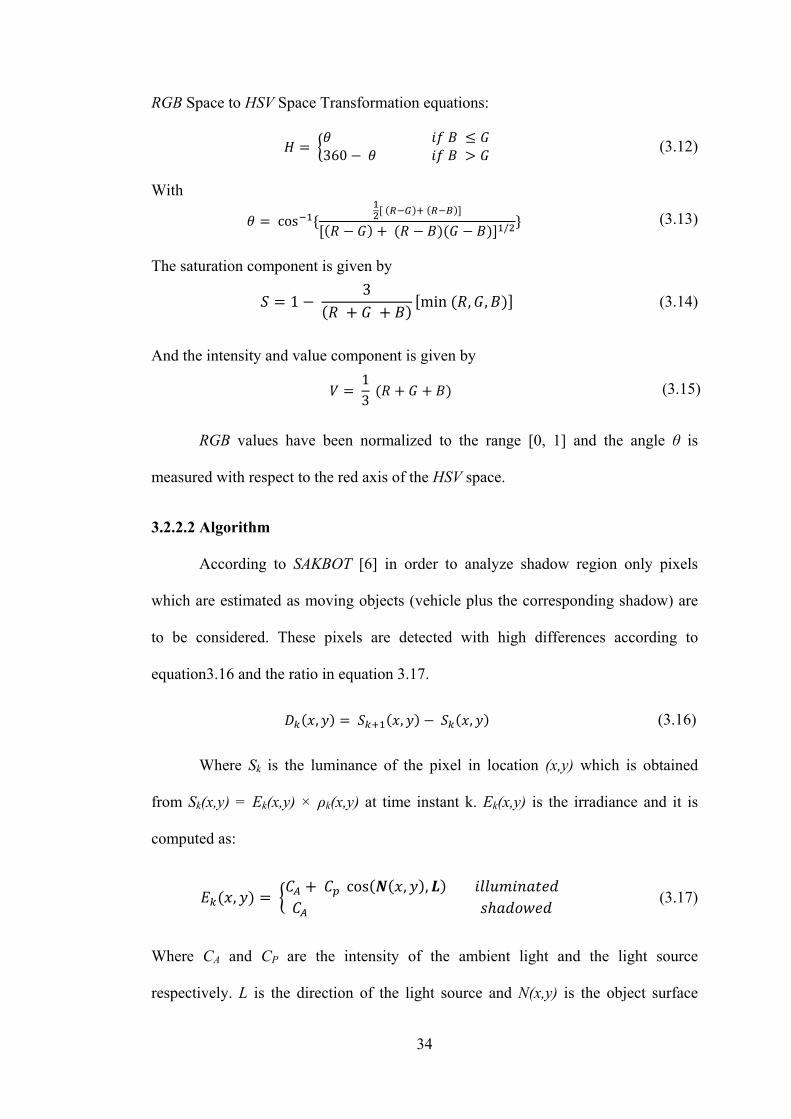
RGB Space to HSV Space Transformation equations: 360 (3.12)
With cos / (3.13)
The saturation component is given by 1 3 min , , (3.14)
And the intensity and value component is given by 13 (3.15)
RGB values have been normalized to the range [0, 1] and the angle θ is
measured with respect to the red axis of the HSV space.
3.2.2.2 Algorithm
According to SAKBOT [6] in order to analyze shadow region only pixels
which are estimated as moving objects (vehicle plus the corresponding shadow) are
to be considered. These pixels are detected with high differences according to
equation3.16 and the ratio in equation 3.17.
, , , (3.16)
Where Sk is the luminance of the pixel in location (x,y) which is obtained
from Sk(x,y) = Ek(x,y) × ρk(x,y) at time instant k. Ek(x,y) is the irradiance and it is
computed as:
, cos , , (3.17)
Where CA and CP are the intensity of the ambient light and the light source
respectively. L is the direction of the light source and N(x,y) is the object surface

35
normal. ρk(x,y) is the reflectance of the object surface. Firstly it is assumed that the
light source is strong, second camera and background are static which would result in
static reflection ρ(x,y) and third, background is planar.
Local appearance changes due to cast shadows can be computed by ratio
Rk(x,y) in equation 3.18.
, ,, (3.18)
This ratio is less than one for shadow pixels. In fact cast shadow pixels
darken the background image but vehicle pixels may or may not darken the
background depending on the object color. Another interesting point is that shadows
often lower the saturation of the pixels.
If in equation 3.18 Sk(x,y) is approximated with intensity value (V-
component) of the pixel in the HSV color space at location (x,y) in the time instant k,
then a shadow point mask SPk(x,y) for each pixel can be defined as :
, 1 ,, , , | , , |0 (3.19)
Where , , , , , are HSV components of the input frame at time
instant k and location (x,y) and , , , , , are HSV components of
the background frame at time instant k and location (x,y).
Figure 3.13 (a) below shows one selected frame from the Yeni-İzmir junction
of Famagusta with its corresponding shadows and Figure 3.13 (b) depicts the HSV
detected shadows for this frame. Similarly Figure 3.14 shows the foreground and
segmented shadow regions for a selected frame of the Highway-I test sequence from
VISOR.

36
(a) (b)
Figure 3. 13: Shadow mask of a video frame at a junction in Famagusta
(a) Foreground with its corresponding shadow, (b) Shadow Point Mask
(a) (b)
Figure 3. 14: Shadow mask of highway-I video [56]
(a) Foreground with its corresponding shadow, (b) Shadow Point Mask
In equation 3.19 the lower bound α is used to define a minimum value for the
darkening effect of shadows on the background and it is almost proportional to the
light source intensity and the upper bound β prevents the system from identifying
noise which slightly changes the background in the shadow regions.
It has been shown that the chrominance values for both the shadow and non-
shadow pixels would vary only slightly. The choice of τH and τS is done according to
this assumption. This choice is complicated and the threshold values have to be
chosen by trial and error.

37
As shown in Figure 3.15 (d) once the shadow pixels are detected and
suppressed the new foreground would only contain the moving vehicles.
(a) (b)
(c) (d)
Figure 3. 15: HSV color space result on shadow removal purpose
(a) Input Frame, (b) Estimated Background, (c) Extracted Foreground (d) shadow removed foreground
3.3 Hybrid color and Texture Based Shadow Removal
In this statistical approach it is assumed that irradiation consists of only one
light source and the chromaticity in the shadow region should be the same as when it
is directly illuminated. A hybrid color and texture model is employed to assist
distinguishing of shaded backgrounds from the ordinary background or of moving
FG objects.

38
3.3.1 Color Based Analysis
The hybrid color technique proposed in [26] makes use of the RGB color
space. In the RGB domain ambient light is ignored and RGB space is invariant to
changes of surface orientation relatively to the light source.
On perfectly matte surfaces, the perceived color is the product of illumination
and surface spectral reflectance [26]. Therefore, if a method could separate the
brightness from the chromaticity component then the observation will be
independent of illumination changes. Figure 3.16 illustrates the color model in three
dimensional RGB space.
Figure 3. 16: Distortion measurements in the RGB Space
Here, foreground denotes the RGB value of a foreground pixel in the incoming frame
and background is of its background counterpart.
To detect the shadow due to illumination on matte surface the distortion of
input frame from background frame can be measured. This distortion is decomposed
to Brightness Distortion and Chromaticity Distortion. [26].
3.3.1.1 Brightness Distortion
Brightness Distortion (BD) is a scalar value that brings the observed color
close to the expected chromaticity line. It is obtained by minimizing (3.20)

39
α represents the pixels brightness strength with respect to an expected value.
α is “1” if the brightness of given pixel in the input frame is the same as in
background frame. α is less than “1” if it is darker than background frame and it is
greater than “1” if it becomes brighter than expected brightness.
Figure 3. 17: Brightness distortion of a traffic scene
3.3.1.2 Chromacity Distortion
Chromaticity distortion is defined as the orthogonal distance between the
observed color and the expected chromaticity line.
CD = || Input frame – α. estimated background || (3.21)
Figure 3. 18: Chromaticity distortion for a sample scene

40
Given the RGB values of a pixel in the input frame as (RI,GI,BI) and
background counterpart frame as (RB ,GB ,BB) the brightness distortion, BD, can be
computed as [24] :
(3.22)
Where α, β and γ are the weights accounting for the influence of R, G and B color
components and has been computed making use of RGB to YUV conversion
equations for the luminance component. Y = α×R + β×G + γ×B , with α = 0.299, β
=0.587, γ = 0.114.
Consequently, a set of thresholds as shown by Table 3.1 are defined to
classify the normalized pixels as foreground, shadow or highlights.
Table 3. 1: Shadow and highlight detection thresholds
If CD < 10 then
If .5<BD<1 then
SHADOW
Else if 1<BD<1.25 then
HIGHLIGT
Else
FOREGROUND
Output obtained by applying the brightness distortion equation is the detected
foreground and shadowed background regions. Parts of FG object pixels may be
misdiagnosed and removed or they may contain some shadow pixels detected as
foreground pixels.

41
3.3.2 Texture Based Analysis
Similar to the color based shadow removal; a texture distortion measure can
be defined to detect possible shadow pixels. A simple way of computing the texture
is to use the first order spatial derivatives; though other more sophisticated measures
can also be employed. We apply Sobel filters in horizontal and vertical directions to
both the background and incoming frame and then compute the Euclidean distance
between them. If this distance is lower than a certain threshold, i.e. very similar
texture, then it is highly likely that the pixels are part of a shadowed region.
Figure 3. 19: Mask of texture based analysis
3.3.3 Morphological Reconstruction
Mathematical morphological theories can be employed in order to reconstruct
the original image without cast shadows or highlights.
By applying BD and CD Thresholds to the pixels of the input frame, a coarse
approximation of foreground object is obtained. While doing morphological
reconstruction the estimation of foreground object is called “Marker”. The so called
“Marker” image is a binary image where a pixel is set to “1” when it corresponds to
a foreground (none cast shadow/highlight pixels). In addition to the marker a “Mask”
is also generated that contains “1” for pixels which have different texture from the
background. These pixels are an approximation of the foreground pixel edge

42
information. A logical AND is applied to the Marker and Mask images and the result
is edge information of object whose shadows are mostly removed. A morphological
dilation is employed to connect vehicle edges together to improve final edge
detection of the foreground object.
_ , (3.22)
Here, SE is the structuring element for dilation purpose and it depends on the size of
foreground to be detected. In this research SE is a box of size (3,3).
Figure 3. 20: Morphological AND result
After small objects are removed by means of a BWAREAOPEN(.) command
in MATLAB, a convex hull approach is used to determine the detected foreground
object precisely. Result of applying the above described method to an outdoor scene
is depicted in Figure 3.21.
Figure 3. 21: Detected foreground with shadows removed

43
3.4 Evaluation
To have a precise comparison between shadow removal algorithms ground
truths video sequences are necessary to provide some quantitative measurements.
Although vision based judgment gives a quick idea about the performance of the
algorithms it is not an approach that is as accurate as the metric based ones.
3.4.1 Ground Truth Frames
Ground Truth video sequences are generally used for quantitative comparison
of different algorithms that try to perform a special task. Video sequences for
outdoor traffic are available from Video Surveillance Online Repository (VISOR)
[56]. In these video sequences some pre-selected frames have the shadow and object
pixels pre-identified and represented with different colors in a mask. This enables the
researchers to test how well their methods are performing in comparison to the ideal
case: in this case the ground truth.
In this study to compare the three different shadow removal algorithms two
sets of highway video sequences were used along with their corresponding ground
truths. The selected test sequences were Highway I and Highway-II from VISOR
[56]. A typical frame and its corresponding ground-truth from Highway-I sequence is
shown by Figure 3.22.

44
(a) (b)
Figure 3. 22: Ground Truth video sequence for shadow removal evaluation, Highway- I video sequence [56]
(a) A typical frame (b) vehicles and corresponding shadow regions
As can be seen from Figure 3.22 (b) the cast shadow regions in the frames
have been marked by red color in the entire frame. This color has been specifically
chosen so as not to mix with the colors of the recorded scene. This provides the
flexibility to simply take the output of the tested shadow detection method and
compare the pixels the method selects against the pixels denoted by red.
Performance comparisons are done by computing two separate scales that are called
precision and recall. The following section gives details about what each scale really
means.
3.4.2 Recall & Precision
3.4.2.1 Recall
Recall is a measure of completeness and is defined as number of true
positives divided by the total number of elements that actually belong to the
foreground- objects (i.e. some of both true positives and false negatives).
(3.24)

45
(3.25)
True Positive (TP) represents the number of foreground pixels correctly
detected by the algorithm. False Positive (FP) represent for the number of pixels
which are incorrectly classified as foreground objects. False Negative (FN) stands for
the number of pixels corresponding to shadow pixels which are misclassified as part
of foreground object.
3.4.2.2 Precision
Precision is a measure of exactness or fidelity. It is evaluated through
dividing the number of items (foreground objects) correctly detected by the total
number of pixels classified as foreground by algorithm.
(3.26)
(3.27)
3.4.3 Data Analysis
The precision and recall values obtained by the evaluation of the shadow
detection routines indicate that shadow removal in HSV color space is the most
precise method. The precision value of the method means that 82.59 % of the
detected foreground objects pixels after shadow removal are actual foreground
pixels.
Table 3. 2: Recall and Precision for different shadow removal algorithms
Precision Recall
HSV Color Space Based 82.59 % 50.88 %
SCS Based 63.28 % 66.29 %
Color & Texture Based 68.34 % 53.86 %

46
CHAPTER 4
LICENSE PLATE RECOGNITION
4.1 Introduction
Automatic license plate recognition (LPR) plays an important role in
detecting vehicles disobeying red lights at junctions. A plate is a label attached to
vehicles in order to distinguish them according to certain rules of each government.
In general license plates consist of alphabetical characters and numbers with different
sizes and colors.
Figure 4. 1:Examples of Mediterranean license plates
License plates in Turkish Republic of Northern Cyprus (TRNC) have five
characters, except for taxis and rent cars which have six or seven characters. The first
two characters of the license plate are alphabets and the last three characters are
numbers. In addition, the front plate is colored in white and black and the rear plate
is colored in yellow and black. These features can be utilized during the license plate
locating procedure. License plates are divided into two categories: single line and
double line of characters. Digits cover most width and heights of the plate region.
Every digit is made of a single block. At times there might be some hyphenation

47
characters between the characters and numbers but these are generally ignored at
segmentation time. Plate size in TRNC for a single line plate is 520 mm × 110 mm
and for double line plate is 340 mm × 220 mm. Some rear private vehicle license
plates are depicted in Figure 4.2 [55].
Figure 4. 2: Samples for single and double line plates in TRNC
4.2 Red Light Tracking and Stop Line Detection
In order to check if there is any red light violators one first needs to determine
the state of the traffic lights. If the junction is monitored by a fixed surveillance
camera then locating the traffic lights in the current input frame turns out to be a
simple crop operation at fixed coordinates. Figure 4.3 below shows three instances of
the traffic lights localized in this manner.
(a) (b) (c)
Figure 4. 3: Traffic Lights
(a) Red: stop (b) Red + Yellow: get ready to go (c) green: go
To determine the state of the traffic light in the current frame color
information from both the YCbCr and HSV color spaces can be combined into a
number of rules as depicted by equation 4.1.

48
110 & 130 & 116 170 0.69 & 0.69 & 0.69
(4.1)
After the color rules are applied and noise like parts are removed connected
component analysis is applied to find out how many color have been detected in each
column. To make the final decision on the state of the light the logical checks shown
below have to be applied.
if (cnt_rt == 1 || cnt_gt ==1 || cnt_ryt == 1)
if (cnt_rt ==1 & cnt_ryt ==1 & sum(sum(gt))<10)
display('Light is red');
end
if (cnt_ryt ==1 & sum(sum(rt)) == 0)
display('Light is yellow');
end
if (sum(sum(gt)) > 10 & cnt_gt==1)
display('Light is green');
end
end
if (cnt_ryt > 1)
display('Light is yellow');
end

49
Once the state of the traffic light has been established a test is carried out to
see if any of the connected components that are in the foreground mask violate an
imaginary stop line or region.
4.3 Algorithm
After a red light violator is detected license plate detection procedure starts.
As demonstrated in Table 4.1 the algorithm for detecting a license plate is developed
in three main parts. The first part is detection and extraction of the plate from the
image containing the vehicle by means of color image processing and plate
properties. The second part of the algorithm is to segment the characters of the
detected license plate region by means of Connected Component Analysis, color and
edge information. Last, a correlation algorithm is used to recognize segmented
characters. The method utilizes template characters and compares their properties
with segmented character properties and decides on the recognition of each character
in turn.
Table 4. 1:License Plate Recognition Steps

50
4.3.1 License Plate Region Locating
4.3.1.1 Radon Transform
As explained in [69], the Hough transform and the related Radon transform
are both able to transform two dimensional images with lines into a domain of
possible line parameters, where each line in the image will give a peak positioned at
the corresponding line parameters. This has lead to many line detection applications
within image processing. In the license plate detection procedure the longest detected
line of the foreground is used to find the object’s skew angle.
Several definitions of the Radon Transform exist, but a very popular form
expresses lines as follows: cos sin (4.1)
Where, θ is the angle and ρ the smallest distance to the origin of the coordinate
system.
Radon transform for a set of parameters (ρ, θ) is the line integral through the
image g(x,y), where the line is positioned corresponding to the value of ( ρ,θ ). The δ
is the Dirac delta function which is infinite for argument 0 and zero for all other
arguments (it integrates to one).
, , (4.2)

51
(a) (b)
(c)
Figure 4. 4: Radon Transform
(a) Foreground, (b) Radon transform of the vehicle, (c) Longest detected line
Figure 4.4 depicts an extracted foreground vehicle and its corresponding
radon transform. It can be seen from Figure 4.4 (b) that some very bright parts are
found in the Radon transform. These parts are the positions of the lines existing in
the original image. A simple threshold algorithm could then be used to select longest
line of the image and compute its angle with the horizontal axis. Once the skew angle
is computed the image can be reverse rotated to make the detected license plate as
horizontal as possible.
4.3.1.2 Yellow Region Extraction
To accomplish the first step of the license plate recognition procedure as
described in Table 4.1, a combination of color and shape information of license plate
is used. After the correction of the skew angle of the detected license plate, an RGB
to HSI transform is employed to help extract all the plate candidates which have

52
yellow color. In the HSI color space the yellow color range in Hue channel is as
shown in Figure 4.5.
Figure 4. 5: Yellow color pixel range in Hue component of HSI color space
Since the aim was to detect red-light violators the frames had been taken from
the back side of the cars and as explained earlier rear plates of cars in TRNC are
yellow. So, plate candidates are regions with yellow color. Subsequently a width to
height ratio (WHR) is considered to verify regions whose aspect ratios were similar
to that of the license plate as shown in Figure 4.6 (b). Finally, an ‘area’ threshold is
used to remove incorrect candidates. Once the correct location of the plate is detected
the extracted RGB plate image is converted to grayscale by RGB2GRAY(.)
command of MATLAB. This eliminates the chrominance components and only
illumination information will remain.

53
(a) (b)
(c) (d)
Figure 4. 6: License plate locating and extraction procedure
(a) Rotated vehicle image (b) width to height ratio filtering (c) locating blob with highest area (d) detected license plate region
To convert the vehicle license plate into a binary image from its gray scale
version, an appropriate threshold is employed. After finding the optimal threshold
which is based on the intensities of different license plate pixels, binary image with
minimum error is obtained.
(a) (b)
Figure 4. 7: Extracted License Plate Region
(a) Gray level license plate, (b) binary license plate with small errors
Applying some morphological operations final binary version of the license
plate can be obtained as depicted in Figure 4.8.

54
Figure 4. 8: Final version of binary license plate
In case no plate region is detected during color image processing, a vertical
edge detection analysis can further be employed on the gray scale version of the
foreground image. In this work the Prewitt method of MATLAB has been used to find
the vertical edges. After discovering the edges, some morphological operations such
as dilation and removal of small unwanted objects are applied. These operations aid
on finding vertical connected edge areas which are license plate region candidates.
Consequently, WHR and area thresholds are applied to extract plate region correctly.
Important steps are demonstrated in Figure 4.9.
(a) (b)
(c) (d)
Figure 4. 9: Vertical edge analysis for license plate detection
(a) An example of gray scale car with white license plate (b) vertical edges of gray scale image (c) Dilated vertical edges obtained from Prewitt Operator (d) detected
LP region after applying WHR and Area thresholds

55
4.3.2 License Plate Character Segmentation
After extracting plate region, next step is to isolate and segment the
characters. Character segmentation is a significant step in license plate recognition
system. There are many difficulties in this step, such as the influence of image noise,
plate frame, rivet, the space mark, plate rotation and illumination variance.
Knowing that all the alphanumeric characters that are used while making
plates consists of only one connected component, a connected component analysis
(CCA) is an efficient method to segment each character or digit. BWLABEL(.)
command in MATLAB is used to perform CCA. Segmented characters for a sample
license plate are shown in Figure 4.10.
Figure 4. 10: Segmented characters of the license plate
4.3.3 License Plate Character Recognition
License plate characters consist of 10 digits and 24 English characters, totally
34 different characters to be recognized. As the English letters or numbers have only
one connected component region, Euler number can be useful to represent the
interior structure.
4.3.3.1 Euler Numbers and Characters
Euler number is a structural property of an image. The Euler number or Euler
characteristics, is defined as the alternating sum of the number of objects in an image
minus the number of holes in it.

56
Figure 4. 11: Euler number example
By calculating Euler number of each segment of the license plate image, it is
possible to distinguish between six different sets of letters and numbers:
• Numbers without holes (Euler = -1)
• Numbers with one hole (Euler = 0)
• Numbers with two holes (Euler = +1)
• Letters without holes (Euler = -1)
• Letters with one hole (Euler = 0)
• Letters with two holes (Euler = 1)

57
Placing Euler number filtering before the character recognition procedure
improves the accuracy of the character recognition and also at the same time speeds
up the processing (fewer comparisons have to be done).
4.3.3.2 Digit Recognition
Before computing any similarity metrics normalization algorithms are applied
to both the template and cropped plate characters to make them similar to each other
in size. Correlation procedure is done by separating all black and white pixels of both
template and cropped plate characters images and counting them separately.
Percentage of black and white pixels in both cropped and template characters are
calculated. The template character which has minimum difference in the percentage
black and white pixels with cropped character is selected to be as the recognized
character. Template characters which are used in this thesis are depicted in Figure
4.12.
Numbers:
Letters:
Figure 4. 12: License plate templates of characters and numbers
4.4 Experimental Examples
Some typical test results of practical implementation of the proposed method
on LPR in which license plates were successfully recognized are shown in Table 4.2.
The method may fail if the video frame is too blurred or if the license plate is highly

58
dirty. Fortunately, pictures were captured by a high resolution camera and they are
clear enough to be detected and recognized by the system with a very high resolution
rate.
Videos are taken from posterior view of the cars where the license plates are
yellow.
Table 4. 2: Practical examples on LPR
Input Frame Extracted foreground LP Region Segmented characters
Recognized
Characters
GE01
9
CJ247
HA335
DM05
3

59
4.5 Comparisons with Previous Departmental Works and Thesis
Related Publications
Similar works on background estimation and foreground segmentation and
violation detection have been done in the electrical and electronics engineering
department of Eastern Mediterranean University by Hüseyin Kusetoğulları [72]
under supervision of Assoc. Prof. Dr. Hasan Demirel and Sevgin Multlu [71] under
supervision of Prof. Dr. Suha Bayındır. Hüseyin has done his research on real time
detection and tracking of vehicles for speed measurement and license plate detection.
As explained in the thesis photos of the over-speeding vehicles containing their
license plate has been captured to be processed later. Their system works in the
temporal domain and uses the frames of the acquired video sequences in order to
detect the presence or absence of a vehicle moving in the road scene. Inter-frame
differencing and background removal methods are employed for the detection of the
vehicle in the frames of the video captured by the camera. Background estimation is
done by simple method of averaging 10 frames of empty scene. A more complete
study on background estimation and subtraction methods has been done by Nima
Seifnaraghi in [70] under supervision of Assoc. Prof. Dr. Erhan A. İnce. Nima has
applied 6 background estimation/subtraction methods for indoor and outdoor
situations. Methods were compared and the fidelity and completeness of the methods
versus each other and speed of them in both outdoor and indoor conditions were
investigated.
Sevgin has added a laser detector to the vehicle speed and license plate
monitoring system to eliminate the disadvantage of the magnetic and fiber optic
detectors.

60
As a result of the research carried out under this thesis two conference
publications were made; one in SIU 2009 and the other in ISCIS 2009. A copy of
these papers can be found in appendices A and B.

61
CHAPTER 5
CONCLUSION AND FUTURE WORK
5.1 Conclusion
The main aim of this research was to develop the essential blocks of a system
that could detect and identify red light violators in the city by the analysis of
surveillance video taken from a fixed video camera. In order to speed up license plate
processing and increase the accuracy of license plate detection it was decided that
first the foreground containing the red light violator(s) would be separated from the
background in the scene. To separate the foreground from the background in the
scene a background subtraction algorithm has to be implemented. In this study a
recently proposed state of the art BG modeling technique known as Group Based
Histogram (GBH) algorithm has been adopted. The GBH is effective and efficient
for building a single Gaussian model of background pixels from traffic image
sequences. This method is reliable against noise and slow moving objects.
Furthermore to eliminate any cast shadows that may be included in the
segmented out foreground three different shadow removal algorithms are introduced
and compared against each other with standard and custom taken video sequences.
First method for shadow detection was based on the Shadow Confidence Score (SCS)
computation discussed in chapter 3. Second shadow removal algorithm used the HSV

62
color space to eliminate shadow pixels from the extracted FG. Final method on
shadow removal used a hybrid approach exploiting the color and texture properties
of BG and input frame to distinguish shaded BG from ordinary BG or moving FG
objects. The tests carried out using ground truth frames for the Highway-I test video
sequence indicated that the HSV based shadow removal would give the best results.
In fact the precision value computed for this method was 0.8259 and the next closer
method had a precision value of 0.6834.
Before searching for a red light violator in the FG masked input frame, the
state of the traffic light should be determined. In this study the traffic lights analysis
was carried out using the YCbCr and HSV color components together with tripwire
processing. In Tripwire systems the camera is used to simulate usage of a
conventional detector by using small localized regions of the image as detector sites.
The simulation results indicate that 99.5% of the time the traffic lights were detected
correctly.
Finally, a correlation based LPR algorithm was used to recognize the
violator’s plate number. First the Radon transform was applied to estimate the skew
angle of the detected foreground objects and rotation angles were corrected. Then a
color and edge based localization for the license plate was carried out. After
localization of the plate the individual characters were segmented out using
connected component analysis and the characters to test were separated based on
their Euler numbers. This was done because Euler number filtering before the
character recognition procedure is known to improve the accuracy of the character
recognition and also at the same time speeds up the processing. Experimental results
indicate that even though the recognition part can further be improved most of the

63
time it is sufficient for correctly recognizing the two letters and three digits on the
plates.
5.2 Future Work
Currently only one set of template characters are used while performing
correlation based character recognition. However template characters based on
different fonts and slant angles could be added to the template set to help increase the
recognition accuracy further. Many instances of violations can be recorded (very
difficult without breaking the law) and percentage accuracy figures could be
provided for correctly identifying the violators.
Also since license plates of taxis and rent cars contain six alphanumeric
characters and non-yellow color the routines could be developed to consider these
specific instances. The fact that the first character of taxi’s license plate is “T” and
first character of a rent car is “Z" can be used in distinguishing these types of plates
from the others.

64
APPENDICES

65
Appendix A: Novel Traffic Lights Signaling Technique Based on
Lane Occupancy Rates
Nima Seifnaraghi, Saameh G. Ebrahimi and Erhan A. Ince*
Electrical and Electronic Eng. Dept., Eastern Mediterranean University
Famagusta, North Cyprus, via Mersin 10 Turkey. *e-mail: [email protected]

66

67

68

69
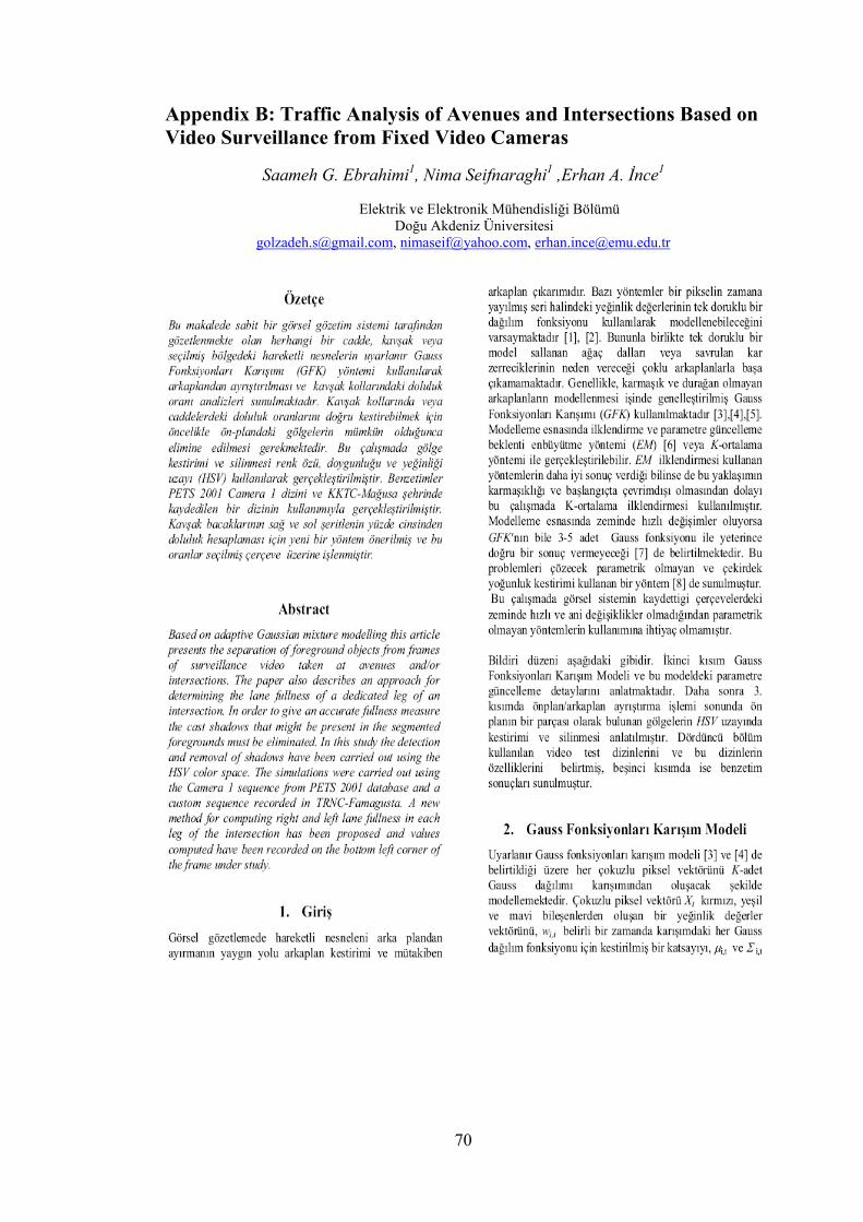
70
Appendix B: Traffic Analysis of Avenues and Intersections Based on Video Surveillance from Fixed Video Cameras
Saameh G. Ebrahimi1, Nima Seifnaraghi1 ,Erhan A. İnce1
Elektrik ve Elektronik Mühendisliği Bölümü Doğu Akdeniz Üniversitesi

71

72

73

74
REFERENCES
[1] W.W. L. Lam, C.C.C. Pang, N.H.C. Yung. “Vehicle Feature Extraction by Patch-
Based Sampling,” Proceedings of SPIE–IS&T Electronic Imaging, Vol. 5022, 2003.
[2] N. Herodotou, K.N. Plataniotis, A.N. Venetsanopoulos, “A color
segmentation scheme for object-based video coding,” in Advances in Digital
Filtering and Signal Processing, pp. 25-29, 1998.
[3] M. Harville, G. Gordon and J. Woodfill, “Foreground segmentation using
adaptive mixture models in color and depth,” in IEEE workshop on detection and
recognition of events in video, pp. 3-11, 2001.
[4] C.Jiang and M.O Ward, “Shadow identification”, Proceeding of IEEE Int’l
Conference on Computer Vision and Pattern Recognition, pp. 606-612, 1992.
[5] A. Prati, I. Mikic, C. Granta, and M.M. Trivedi, “Shadow detection algorithms
for traffic Flow Analysis: a comparative study,” in Proceeding of IEEE Inter. Conf.
on Intelligent Transportation Systems, pp. 340-345, 2001.

75
[6] J. Stauder, R. Mech, and J. Ostermann, “Detection of moving cast shadows for
object segmentation,” IEEE Transactions on Multimedia, vol. 1, no. 1, pp. 65-76,
1999.
[7] M. Kilger, “A Shadow handler in a video-based real-time traffic monitoring
system,” Proceedings of IEEE Workshop on Applications of Computer Vision, pp.
11-18, 1992.
[8] G.G. Sexton and X. Zhang, “Segmentation of shadows for improved object
discrimination,” in Proc. IEEE Colloq. Image Processing for Transport Applications,
pp. 9/1-9/6, 1993.
[9] R. Cucchiara, C. Grana, M. Piccardi, and A. Prati, “Detecting objects, shadows
and ghosts in video streams by exploiting color and motion information,” in
Proceeding of the IEEE Int’l Conference on Image analysis and processing, to
appear. pp. 360-365, 2001.
[10] R.C Jain, “Difference and accumulative difference pictures in dynamic scene
analysis,” Image and Vision Computing, vol. 2, no. 2, pp. 99-108, May 1984.
[11] R. Cucchiara, M. Piccardi, and P. Mello, “Image analysis and rule-based
reasoning for a traffic monitoring systems” IEEE Transaction on Intelligent
Transportation Systems, vol. 1, no. 2 pp 119-130, 2000.

76
[12] A. Neri, S. Colonnese, G. Russo, and P. Talone, “Automatic moving object and
background separation,” Signals Processing, Vol: 66, no: 2, pp. 219-232, 1998.
[13] R. Cucchiara, C. Grana, M. Piccardi, and A. Prati, “Statistical and knowledge-
based moving object detection in traffic scene,” in Processings of IEEE Int’l
Conference on Intelligent Transportation Systems, , pp. 27-32, 2000.
[14] A. Bainbridge-Smith and R.G. Lane, “Determining optical flow using a
differential method,” Image and Vision Computing, vol. 17, pp. 11-22, 1997.
[15] I. Mikic, P. Cosman, G. Kogut, and M.M. Trivedi, “Moving shadow and object
detection in traffic scenes,” in Proceedings on Int’l Conference on Pattern
Recognition, vol. 1, pp. 321 – 324, 2000.
[16] I. Haritoglu, D. Harwood, and L.S. Davis, “W4: real-time surveillance of people
and their activities,” IEEE Transaction on Pattern Analysis and Machine
Intelligence, vol. 22, no. 8, pp. 809-830, 2000.
[17] D. Koller, K. Daniilidis,, and H.H Nagel, “Model-based object tracking in
monocular image sewuences of road traffic scenes,” International Journal of
computer Vision, vol. 10, pp. 257-281, 1993.

77
[18] C. Tomasi and T. Kanade, “Detection and tracking of point features,” in
Tech.Rep. CMU-CS-91-132, 1991.
[19] K. Song, J. Tai, “Real-Time Background Estimation of Traffic Imaginary Using
Group Based Histogram,” in Journal of Information Science and Engineering, Vol.
24, pp. 411 – 423, 2008.
[20] J.M. Wangt, Y.C. Chung, C.L. Changt, and S.W. Chen. “Shadow Detection and
Removal for Traffic Images,” Proceedings of the 2004 IEEE, International
Conference on Networking. Sensing & Control Vol.1 pp. 649- 654. 2004.
[21] K. Siala, M. Chakchouk, O. Besbes,F. Chaieb, “ Moving Shadow Detection
with Support Vector Domain Description in the Color Ratios Space,” International
Conference On Pattern Recognition , vol.4, pp. 384-387. 2004.
[22] D. Xu, J. Lid, Z. Liu, X. Tang, “Indoor Shadow Detection for Video
Segmentation,” IEEE International Conference on Multimedia and Expo. Vol.1, pp.
41- 44, 2004.
[23] R. Cucchiara, C.Grana, M. Piccardi, A. Prati, S. Sirotti ,“Improving Shadow
Suppression in Moving Object Detection with HSV Color Information,” in
proceeding of IEEE International Conference on the Intelligent Transportation
Systems, pp. 334-339, 2001.

78
[24] B. Lei, L. Xu, “Real-Time Outdoor Video Surveillance with Robust Foreground
Extraction and Object Tracking via Multi-state Transition management,” pattern
Recognition Letterspp. Vol. 27 1816-1825, 2006.
[25] J. Landabaso, M. Pardas, L. Xu, “Shadow removal with morphological
Reconstruction,” in IEEE International Conference on Acoustics, Speech, and Signal
Processing, (ICASSP '05). Vol. 2, pp. 729- 732, 2005.
[26] T. Horprasert, D. Harwood, L.S Davis, “A statistical approach for real time
robust background subtraction and shadow detection,” in proceeding of IEEE
ICCV’99 Frame-Rate Workshop, Corfu, Greece,1999.
[27] Z. Yan, H. Zhang, H. Meng, “Cast Vehicle Shadow Segmentation Based on
contour Analysis,” Processing of the 2007 IEEE Intelligent Transportation Systems
Conference pp. 866-871, 2007.
[28] M. Xiao, C. Han, L. Zhang, “Moving Shadow Detection and Removal for
Traffic Sequences,” International Journal of Automation and Computing, pp 38 – 46,
2007.
[29] E. Salvador, a. Cavallaro, T. Ebrahimi, “Shadow Identification and
Classification Using Invariant Color Models,” in Acoustics, Speech, and Signal

79
Processing, (ICASSP '01). 2001 IEEE International Conference, vol. 3, pp. 1545-
1548, 2001.
[30] H. Mahini, S. Kasaei, , F. Dorri, F. Dorri, “An Efficient Features–Based License
Plate Localization Method” In: Proc. of IEEE Int. Conf on Pattern Recognition
ICPR. 2006
[31] R. Parisi, E.D. Di. Claudio, E.D. Lucarelli, G. Orlandi, G, “Car plate recognition
by neural networks and image processing” in Proc. IEEE Int. Symp. Circuits and
Systems, vol. 3, pp. 195–198, 1998.
[32] O. O. V. Villegas, D.l.G. Balderrama, H.J. O. Domínguez, V.G.C. Sánchez,
“License Plate Recognition Using a Novel Fuzzy Multilayer Neural Network”,in
International Journal Of Computers, Vol. 3, 2009.
[33] Z. Ji-yin, Z. Rui-rui, L. Min, L. Yin, “License Plate Recognition Based on
Genetic Algorithm,” in International Conference on Computer Science and Software
Engineering, vol.1, pp. 965-968, 2008.
[34] K.K. Kim, K.I. Kim, J.B. Kim, H.J. Kim, “Learning-based approach for license
plate recognition,” in Neural Networks for Signal Processing X, Vol. 2, pp. 614 -
623, 2000.

80
[35] H. Caner, H.S Gecim, A.Z. Alkar, “Efficient Embedded Neural-Network-Based
License Plate Recognition System,” IEEE Transaction on Vehicular Technology,
Vol. 57, pp. 2675 – 2683, 2008.
[36] B. Hongliang, L. Changping, “A hybrid license plate extraction method based
on edge statistics and morphology,” in 17th International Conference on Pattern
Recognition (ICPR’04), vol.2, pp. 831–834, 2004.
[37] T. Shuang-tong, L. Wen-ju, “Number and Letter Character Recognition of
Vehicle License Plate Based on Edge Hausdorff Distance,” in Proceedings of the
Sixth International Conference on Parallel and Distributed Computing Applications
and Technologies, pp. 850 – 852, 2005.
[38] Y. Cui, Q. Huang, “Character extraction of license plate recognition technology
for toll violation enforcement,” in Inst. Elect. Eng. Colloquium Image Analysis for
Transport Applications, vol.7, pp.1 –5, 1990.
[39] C. Yu, M. Xie, J. Qi, “ A novel System Design of License Plate Recognition,” in
International Symposium on Computational Intelligence and Design, vol.2, pp 114-
117, 2008.

81
[40] Sh.Y. Elhabian, Kh.M. El-Sayed, S.H. Ahmed, “Moving Object Detection in
Spatial Domain using Background Removal Techniques State-Of-Art,” in Recent
Patents on Computer Science Vol.1, pp.32-54, 2008.
[41] N. Oliver, B. Rosario, A. Pentland, “A Bayesian computer vision system for
modeling human interactions,” IEEE Transactions on Pattern Analysis and Machine
Intelligence, vol. 22, pp. 831-843, 2000.
[42] I. Haritaoglu, D. Harwood, and L. Davis, “W4: Real-time surveillance of people
and their activities,” IEEE Transactions on Pattern Analysis and Machine
Intelligence, vol.22, pp. 809-830, 2000.
[43] D.S. Kim, S. I. Krihshnapuram, “Fuzzy decision models in computer vision,” in
Fuzzy sets, Neural Networks, and soft computing, pp. 213 – 232, 1994.
[44] T. Naito, T. Tsukada, K. Yamada, K. Kozuka, and S. Yamamoto, “Robust
license-plate recognition method for passing vehicles under outside environment,”
IEEE Trans.on Vehicle. Technolies., vol. 49, pp. 2309–2319, 2000.
[45] J. A. G. Nijhuis, M. H. T. Brugge, K. A. Helmholt, J. P. W. Pluim, L.
Spaanenburg, R. S. Venema, and M. A. Westenberg, “Car license plate recognition
with neural networks and fuzzy logic,” in Proc. IEEE Int. Conf. Neural Networks,
vol. 5, pp. 2232–2236, 1995.
82
[46] S. K. Kim, D. W. Kim, and H. J. Kim, “A recognition of vehicle license plate
using a genetic algorithm based segmentation,” in Proc. Int. Conf. Image Processing,
vol. 2, pp. 661–664, 1996.
[47] M. H. T. Brugge, J. H. Stevens, J. A. G. Nijhuis, and L. Spaanenburg, “License
plate recognition using DTCNNs,” in Proc. 5th IEEE Int. Workshop on Cellular
Neural Networks and Their Applications, pp. 212-217, 1998.
[48] J. C. H. Poon, M. Ghadiali, G. M. T. Mao, and L. M. Sheung, “A robust vision
system for vehicle license plate recognition using grey-scale morphology,” in Proc.
IEEE Int. Symp. Industrial Electronics, vol. 1, pp. 394–399, 1995.
[49] S. Draghici, “A neural network based artificial vision system for license plate
recognition,” Int. J. Neural Systems, vol. 8, pp. 113–126, 1997.
[50] D. S. Gao and J. Zhou, “Car license plates detection from complex scene,” in
Proc. 5th Int. Conf. Signal Processing, vol. 2, pp. 1409–1414, 2000.
[51] H. A. Hegt, R. J. De la Haye, and N. A. Khan, “A high performance license
plate recognition system,” in Proc. IEEE Int. Conf. System, Man, and Cybernetics,
vol. 5, pp. 4357–4362, 1998.

83
[52] L. Salgado, J. M. Menendez, E. Rendon, and N. Garcia, “Automatic car plate
detection and recognition through intelligent vision engineering,” in Proc. IEEE Int.
Carnahan Conf. Security Technology, pp. 71–76, 1999.
[53] N. Ezaki, M. Bulacu, L. Schomaker, “Text detection from natural scene images:
towards a system for visually impaired persons,” in Pattern Recognition, ICPR 2004.
Proceedings of the 17th International Conference, Vol.2, pp. 683 – 686, 2004.
[54] G.S.K. Fung, N.H.C Yung, G.K.H. Pang, A.H.S. Lai, “Towards Detection of
Moving Cast Shadows for Visual Traffic Surveillance,” in Systems, Man, and
Cybernetics, Vol. 4, pp. 2505-2510, 2001.
[55] License plate recognition, www user survey. Retrieved 4 may 2004. URL:
http://www.worldlicenseplates.com/
[56] Highway-I, Highway-II and ground truth video sequences, found at the ViSOR
repository URL: http://www.openvisor.org/video_categories.asp
[57] AR. Francois, GG. Medioni, “Adaptive color background modeling for real-
time segmentation of video streams,” in Proceedings of the Wireless Sensor
Networks Recent Patents on Computer Science, USA; vol.1, pp.227-232, 2008.

84
[58] S. Huwer, H. Niemann , “Adaptive Change Detection for Real-Time
Surveillance Applications,” Third IEEE Int. Workshop on Visual Surveillance; pp.
37-45, 2000.
[59] RJ. Radke, S. Andra, O. Al-Kofahi, B. Roysam, “Image Change Detection
Algorithms: A systematic survey,” image processing, IEEE Transaction, vol.14, pp.
294-307, March 2005.
[60] C. Stauffer, WEL. Grimson, “Adaptive Background Mixture Models for Real-
Time Tracking,” IEEE Computer Society Conf. on Computer Vision and Pattern
Recognition CVPR,; vol.2, pp. 246-252, 1999.
[61] R. Cutler and L. Davis, “View-based detection,” in Proceedings Fourteenth
International Conference on Pattern Recognition, vol.1, pp. 495-500, (Brisbane,
Australia), Aug 1998
[62] Y.Chung, J.Wang and S.Chen, “Progressive Background Images Generation,”
In Proc. 15th IPPR. Conf. Computer Vision, 2002.
[63] N .McFarlane, C.Schofield , “Segmentation and tracking of piglets in images,”
Machine Vision Application; vol. 83, pp. 187-193, 1995.
[64] C. Wren, A. Azabayejani, T. Darrel, and A. Pentland, “Pfinder: Real-time
tracking of the human body,” IEEE Transactions on Pattern Analysis and Machine
Intelligence, vol.19, pp. 780-785, July 1997.

85
[65] S. Jabri, Z. Duric, H. Wechsler, A. Rosenfeld, “Detection and Location of
People in Video Images Using Adaptive Fusion of Color and Edge Information,”
ICPR, 15th Int. Conf. on Pattern Recognition; vol.4, pp. 4627-4630, 2000.
[66] J. Rittscher, J. Kato, S. Joga, A. Blake, “A probabilistic background model for
tracking,” In Proc. 6th Eur. Conf. Computer Vision, vol.2, pp. 336-350, 2000.
[67] N. Friedman and S. Russell, “Image segmentation in video sequences: a
probabilistic approach,” in Proceedings of the 13th Conference on Uncertainty in
Artificial Intelligence, 1997.
[68] J. Cho, D. Jang, C. Hwang, “Detection of Moving Cast Shadows for Traffic
Monitoring System,” in Ieice Trans. Fundamentals, Vol.E89 – A, No.3, 2006
[69] PhD Thesis, P. Toft, ttp://eivind.imm.dtu.dk/staff/ptoft/Radon/Radon.html, 1996
[70] A comparative study of Background Estimation Algorithms, Nima Seifnaraghi,
Eastern Mediterranean University, September 2009
[71] Detection and Recognition of License Plates of Vehicles Violating The Speed
Limit, Sevgin Mutlu, Eastern Mediterranean University, September 2006
[72] Real Time Detection and Tracking of Vehicles for Speed Measurement and
License Plate Detection, Huseyin Kusetogullari, Eastern Mediterranean University,
July 2007


![Light Space Perspective Shadow Maps · rameterize the shadow map is to tilt or warp the shadow plane directly [CG04, LI03]. Recent approaches propose to combine shadow maps with shadow](https://static.fdocuments.net/doc/165x107/5e37bd5178a8d5075e57de01/light-space-perspective-shadow-maps-rameterize-the-shadow-map-is-to-tilt-or-warp.jpg)