sfm data processing exploration v3 - UNAVCO

Questions or comments please contact education AT unavco.org Version February 17, 2016

Structure from Motion (SfM) Photogrammetry Data Exploration and Processing Manual

Written by Katherine Shervais (UNAVCO) and James Dietrich (Dartmouth)

Collecting data in the field is only the first step in the complete SfM workflow. This manual will take you through the skills needed to complete assignments for Units 1, 2, and 3. These sections are not linked to specific projects, so you will need to use your own judgment on what portions of the manual you need to use for your given assignment. However, the sections on creating a model are required for every unit. You may complete the steps to generate a model or your instructor may complete these steps for you. In addition, you can always use the Help menu in Agisoft Photoscan Pro.

Note: this is accurate as of March 2016 (Agisoft version 1.2). Software updates may result in portions of this manual becoming out-of-date.

I. Basics of Agisoft (interface, etc.) Note: make sure there is room on the computer hard drive for the data. Agisoft project files (.psx’s) can be gigabytes in size. The exported DEMs and orthomosaics are also quite large.

Agisoft has many panes within the main window. The left column contains the Reference pane, which lists the cameras, markers (ground control points) and scale bars. When something in the Reference pane is checked, it is used to georeference the model. The left column is also the Workspace pane (which lists the different parts of the model, like the photos, sparse point clouds, and dense point clouds) and can be toggled by selecting the tab at the bottom of the column. The Model pane shows the model as it is; a tab can also appear here to show the Ortho view. The Ortho view is how you view the products of your model, like the DEM or orthomosaic. The

SfM Data Exploration and Processing Manual


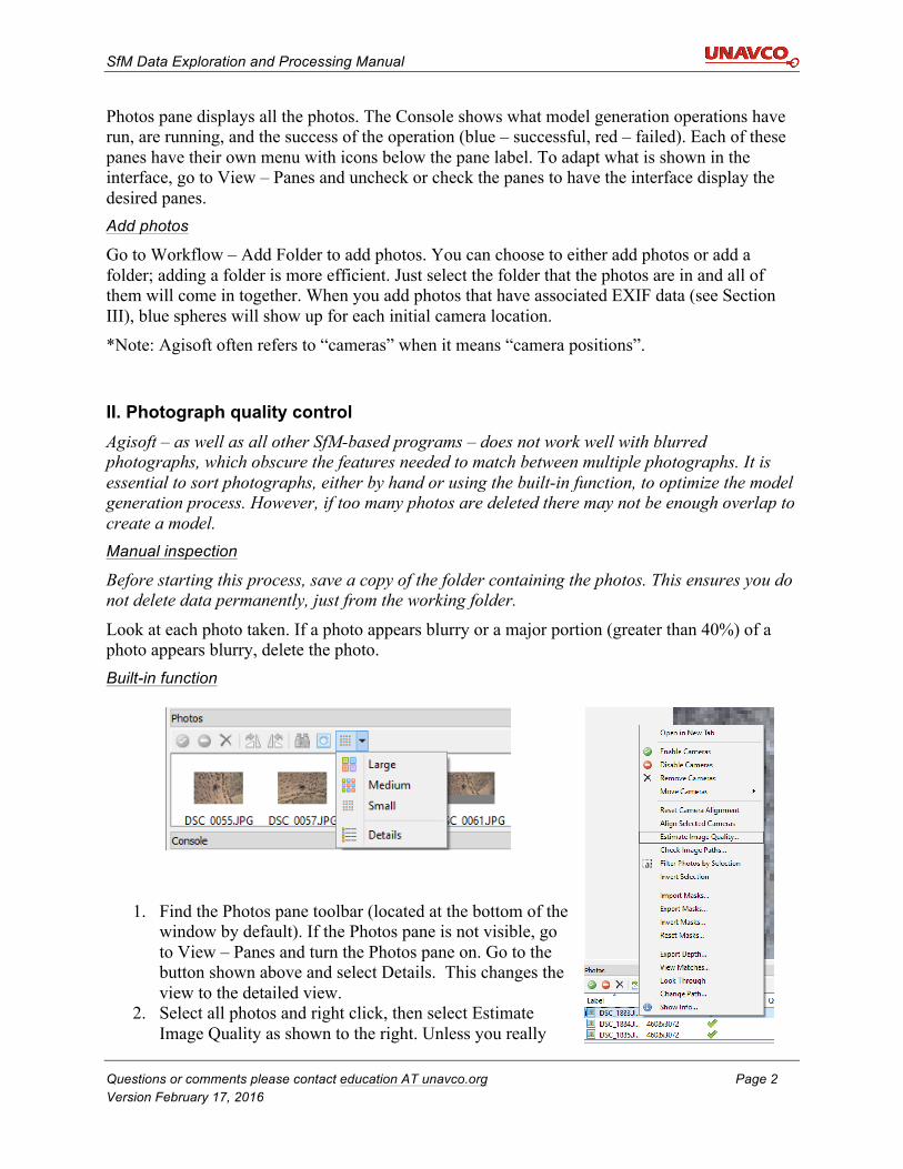
Photos pane displays all the photos. The Console shows what model generation operations have run, are running, and the success of the operation (blue – successful, red – failed). Each of these panes have their own menu with icons below the pane label. To adapt what is shown in the interface, go to View – Panes and uncheck or check the panes to have the interface display the desired panes. Add photos

Go to Workflow – Add Folder to add photos. You can choose to either add photos or add a folder; adding a folder is more efficient. Just select the folder that the photos are in and all of them will come in together. When you add photos that have associated EXIF data (see Section III), blue spheres will show up for each initial camera location. *Note: Agisoft often refers to “cameras” when it means “camera positions”.

II. Photograph quality control Agisoft – as well as all other SfM-based programs – does not work well with blurred photographs, which obscure the features needed to match between multiple photographs. It is essential to sort photographs, either by hand or using the built-in function, to optimize the model generation process. However, if too many photos are deleted there may not be enough overlap to create a model. Manual inspection

Before starting this process, save a copy of the folder containing the photos. This ensures you do not delete data permanently, just from the working folder.

Look at each photo taken. If a photo appears blurry or a major portion (greater than 40%) of a photo appears blurry, delete the photo. Built-in function

1. Find the Photos pane toolbar (located at the bottom of the window by default). If the Photos pane is not visible, go to View – Panes and turn the Photos pane on. Go to the button shown above and select Details. This changes the view to the detailed view.

2. Select all photos and right click, then select Estimate Image Quality as shown to the right. Unless you really



only want to do a subset of the photos, select “All cameras” and “All Frames” in the dialogue box and then click “OK”. Sometimes Agisoft may give you a very long time (hours-days) until completion but generally it will amend that after a few minutes to be a much short time.

3. The column titled Quality shows values from 0 to 1. Agisoft recommends deleting photos with a value below 0.5; other workers suggest removing photos with a value of 0.6 or lower. You can view a given photo in the larger Agisoft pane by double clicking on it in the “Photo” pane. To remove it, select the photo/s you want to remove, right click and select “Remove cameras” (think of this as remove camera position).

Masking photographs

Masks can be used for one of two reasons: a) photos include areas that are not of interest (i.e. the sky) or b) photos contain portions that are blurry, but are primarily clear. Agisoft allows the user to create masks in the program or import masks created in another program. For more details on this process, consult the Agisoft User Manual. Do not crop photos. ONLY mask or delete them.

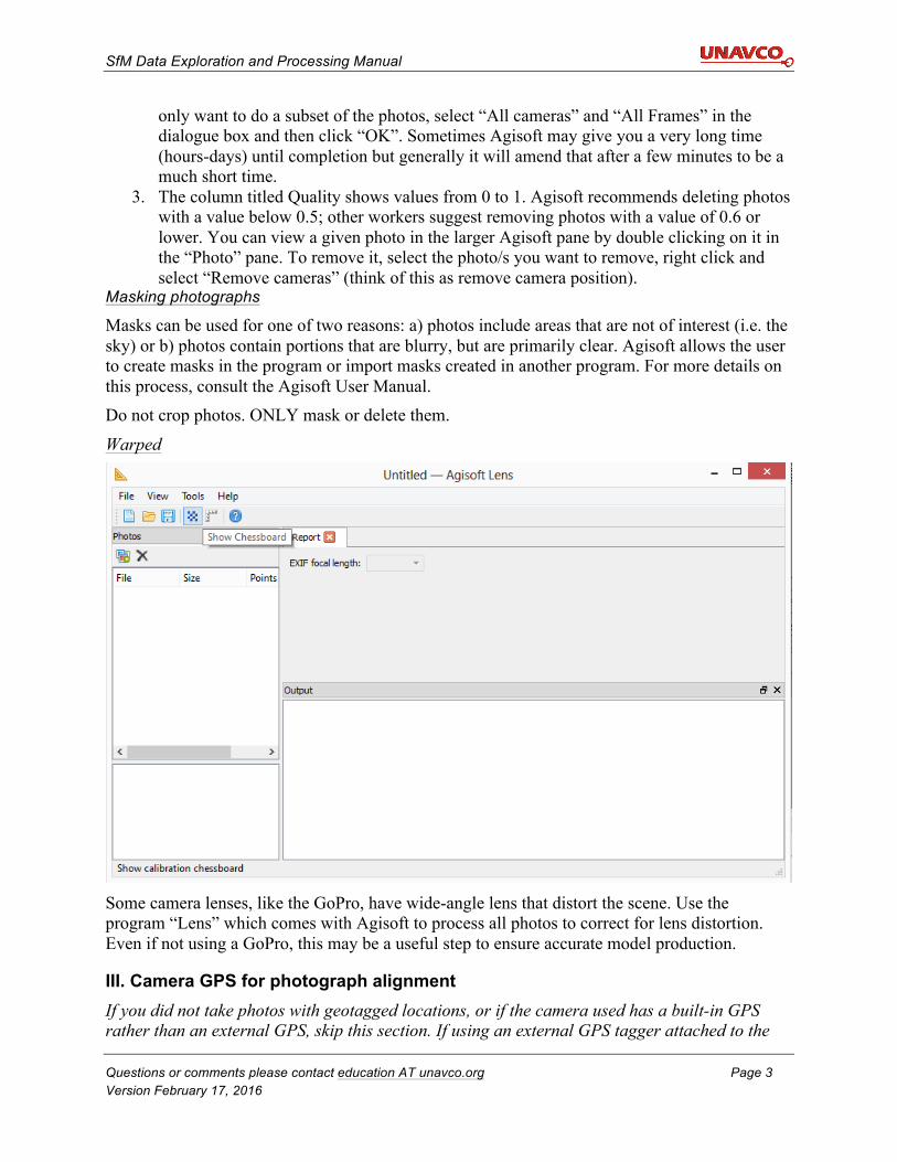
Warped

Some camera lenses, like the GoPro, have wide-angle lens that distort the scene. Use the program “Lens” which comes with Agisoft to process all photos to correct for lens distortion. Even if not using a GoPro, this may be a useful step to ensure accurate model production.

III. Camera GPS for photograph alignment If you did not take photos with geotagged locations, or if the camera used has a built-in GPS rather than an external GPS, skip this section. If using an external GPS tagger attached to the



camera, follow the steps below. Make sure you do this step before starting the model, because the GPS data will expedite the alignment process. If doing a You may do this in an external program (so the data is linked to the photos forever) or in Agisoft (so the data is linked to the photos in the program). Download a program for geotagging

Programs like Geosetter, PhotoLinker, and GPSPhotoLinker take the EXIF data in the photos and embeds the GPS position into the metadata for each photo. Each software package has its own workflow; follow the instructions for the program of choice. In Agisoft

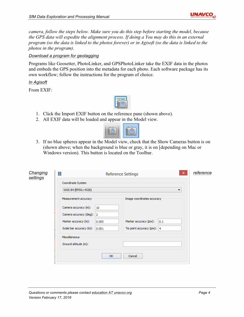
From EXIF:

1. Click the Import EXIF button on the reference pane (shown above). 2. All EXIF data will be loaded and appear in the Model view.

3. If no blue spheres appear in the Model view, check that the Show Cameras button is on (shown above; when the background is blue or gray, it is on [depending on Mac or Windows version). This button is located on the Toolbar.

Changing reference settings



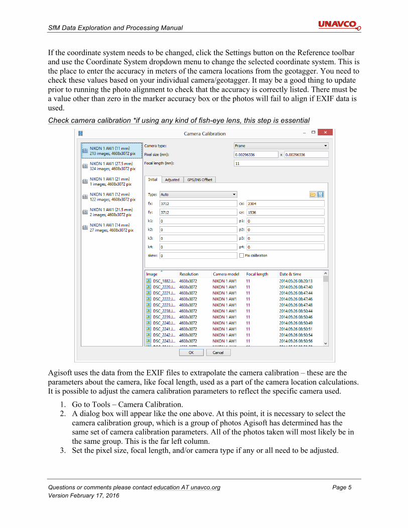
If the coordinate system needs to be changed, click the Settings button on the Reference toolbar and use the Coordinate System dropdown menu to change the selected coordinate system. This is the place to enter the accuracy in meters of the camera locations from the geotagger. You need to check these values based on your individual camera/geotagger. It may be a good thing to update prior to running the photo alignment to check that the accuracy is correctly listed. There must be a value other than zero in the marker accuracy box or the photos will fail to align if EXIF data is used. Check camera calibration *if using any kind of fish-eye lens, this step is essential

Agisoft uses the data from the EXIF files to extrapolate the camera calibration – these are the parameters about the camera, like focal length, used as a part of the camera location calculations. It is possible to adjust the camera calibration parameters to reflect the specific camera used.

1. Go to Tools – Camera Calibration. 2. A dialog box will appear like the one above. At this point, it is necessary to select the

camera calibration group, which is a group of photos Agisoft has determined has the same set of camera calibration parameters. All of the photos taken will most likely be in the same group. This is the far left column.

3. Set the pixel size, focal length, and/or camera type if any or all need to be adjusted.



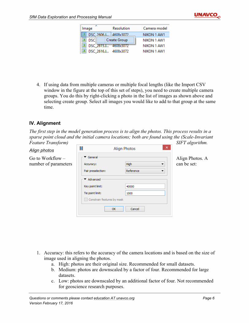
4. If using data from multiple cameras or multiple focal lengths (like the Import CSV window in the figure at the top of this set of steps), you need to create multiple camera groups. You do this by right-clicking a photo in the list of images as shown above and selecting create group. Select all images you would like to add to that group at the same time.

IV. Alignment The first step in the model generation process is to align the photos. This process results in a sparse point cloud and the initial camera locations; both are found using the (Scale-Invariant Feature Transform) SIFT algorithm. Align photos

Go to Workflow – Align Photos. A number of parameters can be set:

1. Accuracy: this refers to the accuracy of the camera locations and is based on the size of image used in aligning the photos.

a. High: photos are their original size. Recommended for small datasets. b. Medium: photos are downscaled by a factor of four. Recommended for large

datasets. c. Low: photos are downscaled by an additional factor of four. Not recommended

for geoscience research purposes.



2. Pair preselection: how Agisoft selects pairs of photos for comparison. a. Disabled: default. Use if no camera geotagging was used. b. Generic: uses lower accuracy first and then higher accuracy second. Use if

aligning photos did not work the first time. This is faster than the disabled setting and will reduce processing by at least two hours for large datasets.

c. Reference: uses camera locations from geotagging as a reference. Recommended; this is faster than the disabled setting and will reduce processing by at least two hours for large datasets.

3. Advanced: generally keep these at default values. a. Key point limit: 40,000 default; if faster processing is required, reduce the

number. HOWEVER, this can lead to aligning photo failure.i. When set to zero, there is no limit.

b. Tie point limit: upper limit for matching points for every image; 1000-2000 is the norm.

i. When set to zero, there is no limit. c. Constrain features by mask: excludes areas covered by masks in camera location

calculations

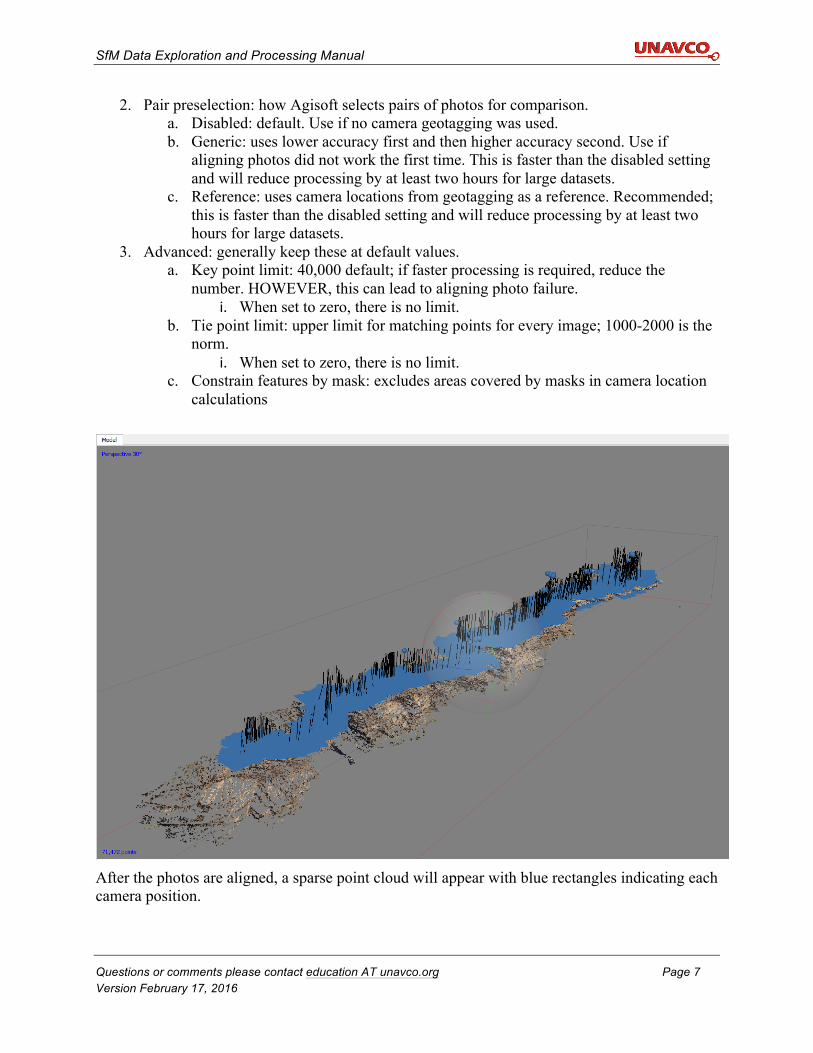
After the photos are aligned, a sparse point cloud will appear with blue rectangles indicating each camera position.



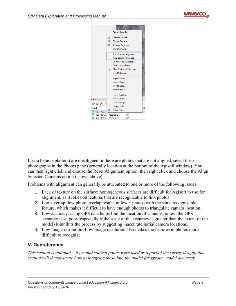
If you believe photo(s) are misaligned or there are photos that are not aligned, select these photographs in the Photos pane (generally location at the bottom of the Agisoft window). You can then right click and choose the Reset Alignment option, then right click and choose the Align Selected Cameras option (shown above). Problems with alignment can generally be attributed to one or more of the following issues:

1. Lack of texture on the surface: homogeneous surfaces are difficult for Agisoft to use for alignment, as it relies on features that are recognizable to link photos.

2. Low overlap: low photo overlap results in fewer photos with the same recognizable feature, which makes it difficult to have enough photos to triangulate camera location.

3. Low accuracy: using GPS data helps find the location of cameras, unless the GPS accuracy is so poor (especially if the scale of the accuracy is greater than the extent of the model) it inhibits the process by suggesting inaccurate initial camera locations.

4. Low image resolution: Low image resolution also makes the features in photos more difficult to recognize.

V. Georeference This section is optional – if ground control points were used as a part of the survey design, this section will demonstrate how to integrate these into the model for greater model accuracy.



Ground control point integration

If you would like to convert the ground control point data to another projection, you may use Agisoft or (recommended) use the VDatum program from NOAA/NGS (http://vdatum.noaa.gov/). The text file for Agisoft should be formatted to have columns for the GCP name, latitude, longitude, and elevation with no other information.

The most important thing for this process is consistency in coordinate systems. It will be impossible for the model to work if multiple coordinate systems are used (one for the EXIF data, one for the GCPs).

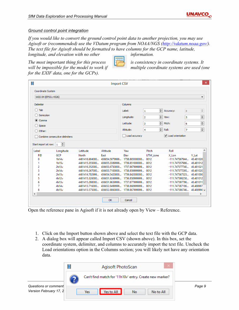
Open the reference pane in Agisoft if it is not already open by View – Reference.

1. Click on the Import button shown above and select the text file with the GCP data. 2. A dialog box will appear called Import CSV (shown above). In this box, set the

coordinate system, delimiter, and columns to accurately import the text file. Uncheck the Load orientations option in the Columns section; you will likely not have any orientation data.



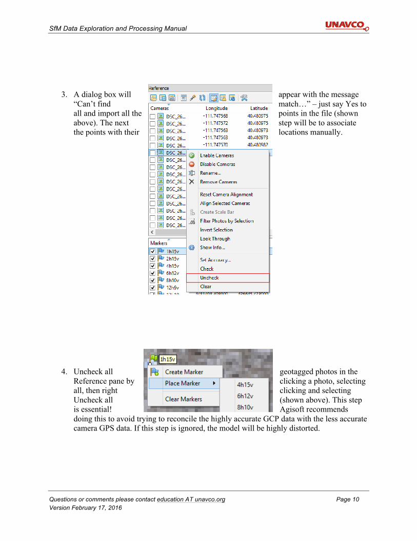
3. A dialog box will appear with the message

“Can’t find match…” – just say Yes to all and import all the points in the file (shown above). The next step will be to associate the points with their locations manually.

4. Uncheck all geotagged photos in the

Reference pane by clicking a photo, selecting all, then right clicking and selecting Uncheck all (shown above). This step is essential! Agisoft recommends doing this to avoid trying to reconcile the highly accurate GCP data with the less accurate camera GPS data. If this step is ignored, the model will be highly distorted.



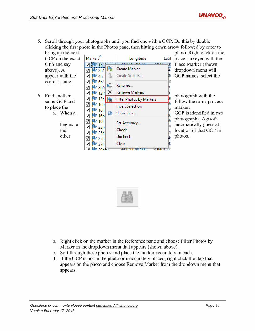
5. Scroll through your photographs until you find one with a GCP. Do this by double

clicking the first photo in the Photos pane, then hitting down arrow followed by enter to bring up the next photo. Right click on the GCP on the exact place surveyed with the GPS and say Place Marker (shown above). A dropdown menu will appear with the GCP names; select the correct name.

6. Find another photograph with the same GCP and follow the same process to place the marker.

a. When a GCP is identified in two photographs, Agisoft

begins to automatically guess at the location of that GCP in other photos.

b. Right click on the marker in the Reference pane and choose Filter Photos by Marker in the dropdown menu that appears (shown above).

c. Sort through these photos and place the marker accurately in each. d. If the GCP is not in the photo or inaccurately placed, right click the flag that

appears on the photo and choose Remove Marker from the dropdown menu that appears.



7. Find the photos pane and click the Reset Filter button shown above. 8. Start the process over from step 5 for two more markers.

9. Click the Update button in the Reference pane to roughly georeference the model based

on these points. This will expedite the process of placing the remaining GCPs. 10. Repeat steps 6b to 9 for all remaining markers.

*note: the Agisoft user manual suggests a slightly different process for integrating GCPs; each produce the same result but this process is a bit more intuitive.

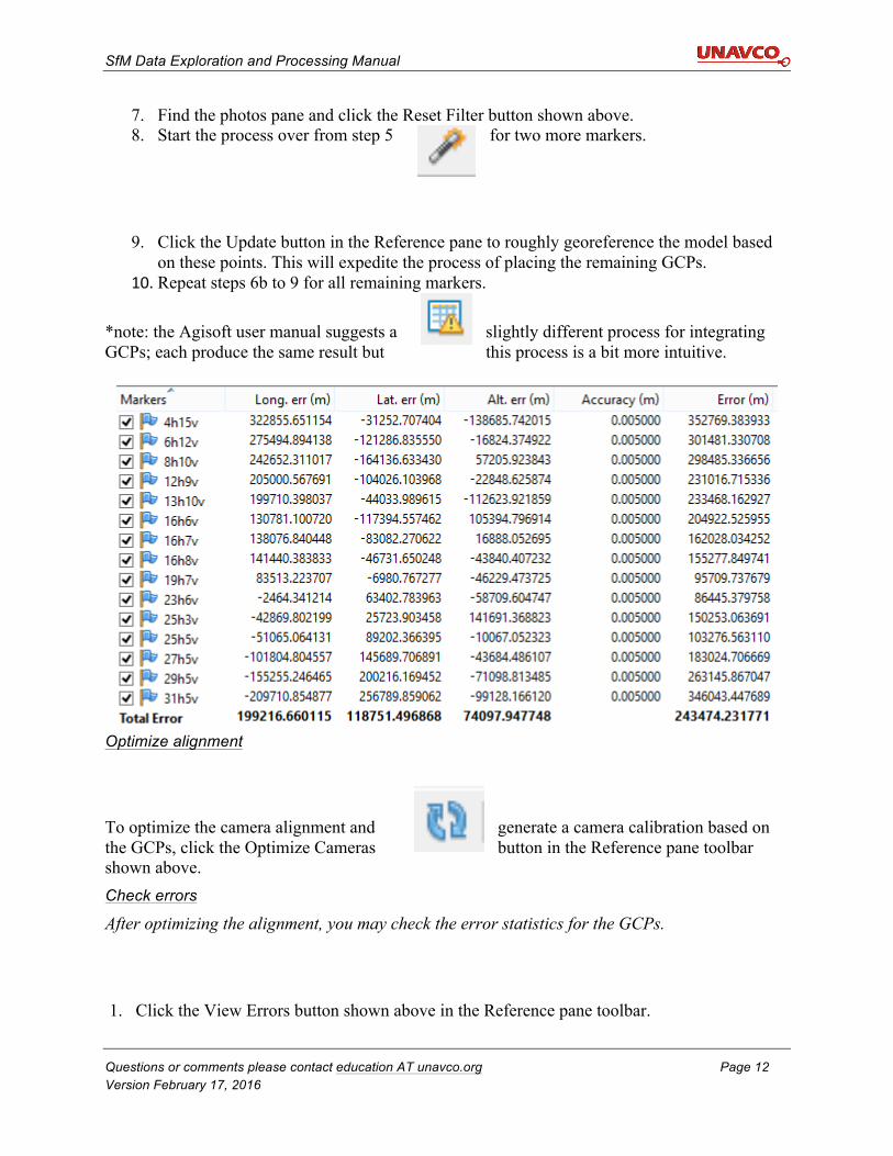
Optimize alignment

To optimize the camera alignment and generate a camera calibration based on the GCPs, click the Optimize Cameras button in the Reference pane toolbar shown above. Check errors

After optimizing the alignment, you may check the error statistics for the GCPs.

1. Click the View Errors button shown above in the Reference pane toolbar.



2. Expand the width of the pane to see the Error column, which gives the root sum of squares error for each point. The row titled Total Error gives the root mean squared errors for the easting, northing, and altitude columns for all points. The example above has very large error estimates.



VI. Build dense point cloud This step uses the camera locations and the sparse point cloud to generate a dense point cloud. Check the bounding box

Occasionally, the bounding box around the model crops out portions of the sparse point cloud. If this is the case, use the Resize Region and Rotate Region tools to resize the bounding box area. This is also useful if you would like to crop the point cloud to include less data, which makes the processing of the dense point cloud faster. Dense point cloud

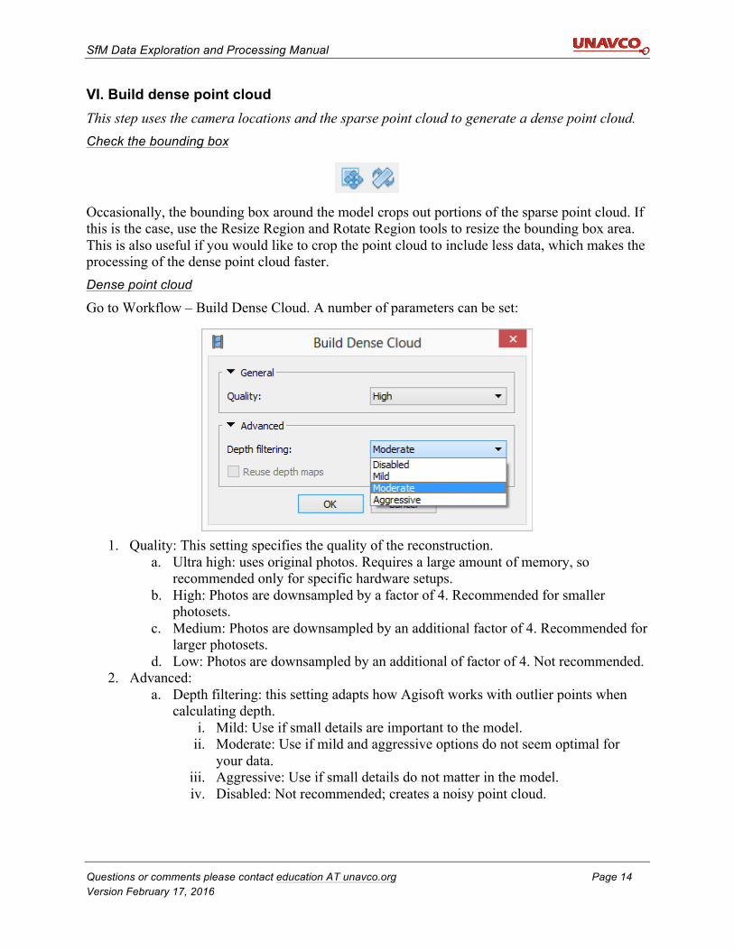
Go to Workflow – Build Dense Cloud. A number of parameters can be set:

1. Quality: This setting specifies the quality of the reconstruction.

a. Ultra high: uses original photos. Requires a large amount of memory, so recommended only for specific hardware setups.

b. High: Photos are downsampled by a factor of 4. Recommended for smaller photosets.

c. Medium: Photos are downsampled by an additional factor of 4. Recommended for larger photosets.

d. Low: Photos are downsampled by an additional of factor of 4. Not recommended. 2. Advanced:

a. Depth filtering: this setting adapts how Agisoft works with outlier points when calculating depth.

i. Mild: Use if small details are important to the model. ii. Moderate: Use if mild and aggressive options do not seem optimal for

your data. iii. Aggressive: Use if small details do not matter in the model. iv. Disabled: Not recommended; creates a noisy point cloud.



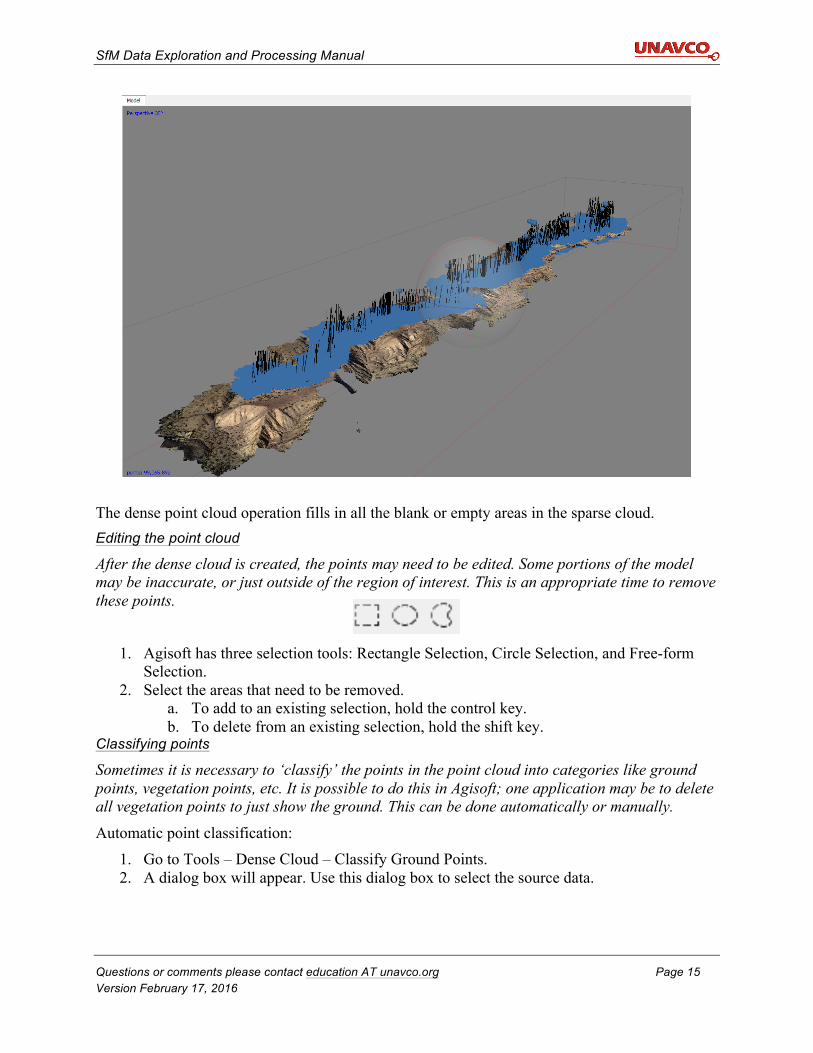
The dense point cloud operation fills in all the blank or empty areas in the sparse cloud. Editing the point cloud

After the dense cloud is created, the points may need to be edited. Some portions of the model may be inaccurate, or just outside of the region of interest. This is an appropriate time to remove these points.

1. Agisoft has three selection tools: Rectangle Selection, Circle Selection, and Free-form Selection.

2. Select the areas that need to be removed. a. To add to an existing selection, hold the control key. b. To delete from an existing selection, hold the shift key.

Classifying points

Sometimes it is necessary to ‘classify’ the points in the point cloud into categories like ground points, vegetation points, etc. It is possible to do this in Agisoft; one application may be to delete all vegetation points to just show the ground. This can be done automatically or manually.

Automatic point classification: 1. Go to Tools – Dense Cloud – Classify Ground Points. 2. A dialog box will appear. Use this dialog box to select the source data.



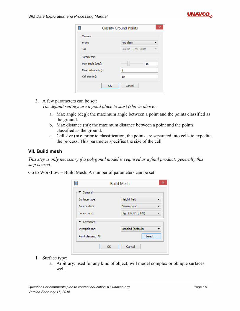
3. A few parameters can be set:

The default settings are a good place to start (shown above). a. Max angle (deg): the maximum angle between a point and the points classified as

the ground. b. Max distance (m): the maximum distance between a point and the points

classified as the ground. c. Cell size (m): prior to classification, the points are separated into cells to expedite

the process. This parameter specifies the size of the cell.

VII. Build mesh This step is only necessary if a polygonal model is required as a final product; generally this step is used.

Go to Workflow – Build Mesh. A number of parameters can be set:

1. Surface type:

a. Arbitrary: used for any kind of object; will model complex or oblique surfaces well.



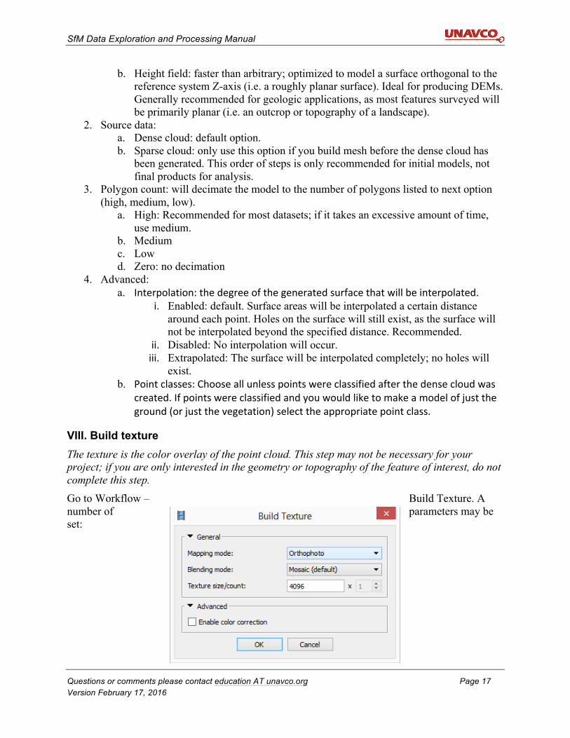
b. Height field: faster than arbitrary; optimized to model a surface orthogonal to the reference system Z-axis (i.e. a roughly planar surface). Ideal for producing DEMs. Generally recommended for geologic applications, as most features surveyed will be primarily planar (i.e. an outcrop or topography of a landscape).

2. Source data: a. Dense cloud: default option. b. Sparse cloud: only use this option if you build mesh before the dense cloud has

been generated. This order of steps is only recommended for initial models, not final products for analysis.

3. Polygon count: will decimate the model to the number of polygons listed to next option (high, medium, low).

a. High: Recommended for most datasets; if it takes an excessive amount of time, use medium.

b. Medium c. Low d. Zero: no decimation

4. Advanced: a. Interpolation:thedegreeofthegeneratedsurfacethatwillbeinterpolated.

i. Enabled: default. Surface areas will be interpolated a certain distance around each point. Holes on the surface will still exist, as the surface will not be interpolated beyond the specified distance. Recommended.

ii. Disabled: No interpolation will occur. iii. Extrapolated: The surface will be interpolated completely; no holes will

exist. b. Pointclasses:Chooseallunlesspointswereclassifiedafterthedensecloudwas

created.Ifpointswereclassifiedandyouwouldliketomakeamodelofjusttheground(orjustthevegetation)selecttheappropriatepointclass.

VIII. Build texture The texture is the color overlay of the point cloud. This step may not be necessary for your project; if you are only interested in the geometry or topography of the feature of interest, do not complete this step. Go to Workflow – Build Texture. A number of parameters may be set:



1. Mapping mode: how the texture will be generated

a. Generic: Uniform texture with no assumptions about the type of scene; best to use if the below options do not fit the feature of interest.

b. Adaptive orthophoto: The feature is assumed to have horizontal and vertical regions and these are textured separately; best results for arbitrary meshes and features (like cliffs and the ground below) with X and Z oriented surfaces.

c. Orthophoto: the feature is assumed to be primarily horizontal; this is best for horizontal outcrops as the texture is not calculated in the Z or elevation orientation.

d. Spherical: objects with a spherical form. Usually not used for geoscience applications.

e. Single photo: select a single photo from the photoset to base all texture on; this is also rarely used.

f. Keep uv: not recommended. 2. Blending mode: how the pixels from different photos of the same feature will be

combined. a. Mosaic: default; blends specific pixels from photo with best representation of

feature with pixels from other images to avoid seams in the texture. Generally recommended.

b. Average: averages all pixels from all photos containing that feature. c. Max intensity: color is chosen from photograph that has maximum intensity for

that pixel. d. Min intensity: color is chosen from photograph that has minimum intensity for

that pixel. e. Disabled: not blended; best photo of each feature is used for the coloration of that

point. 3. Texture size/count: determines the size in pixels of the resultant texture; the higher the

number, the higher the resolution. Use large numbers (4096 x 6, 7, 8) if the texture/orthophoto is the most important feature for your work. Otherwise the standard 4086 pixels is optimal.

4. Advanced: a. Enable color correction: Use when the photoset has extreme brightness variation.



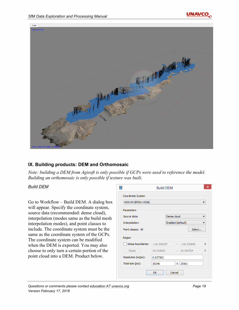
IX. Building products: DEM and Orthomosaic Note: building a DEM from Agisoft is only possible if GCPs were used to reference the model. Building an orthomosaic is only possible if texture was built.

Build DEM

Go to Workflow – Build DEM. A dialog box will appear. Specify the coordinate system, source data (recommended: dense cloud), interpolation (modes same as the build mesh interpolation modes), and point classes to include. The coordinate system must be the same as the coordinate system of the GCPs. The coordinate system can be modified when the DEM is exported. You may also choose to only turn a certain portion of the point cloud into a DEM. Product below.



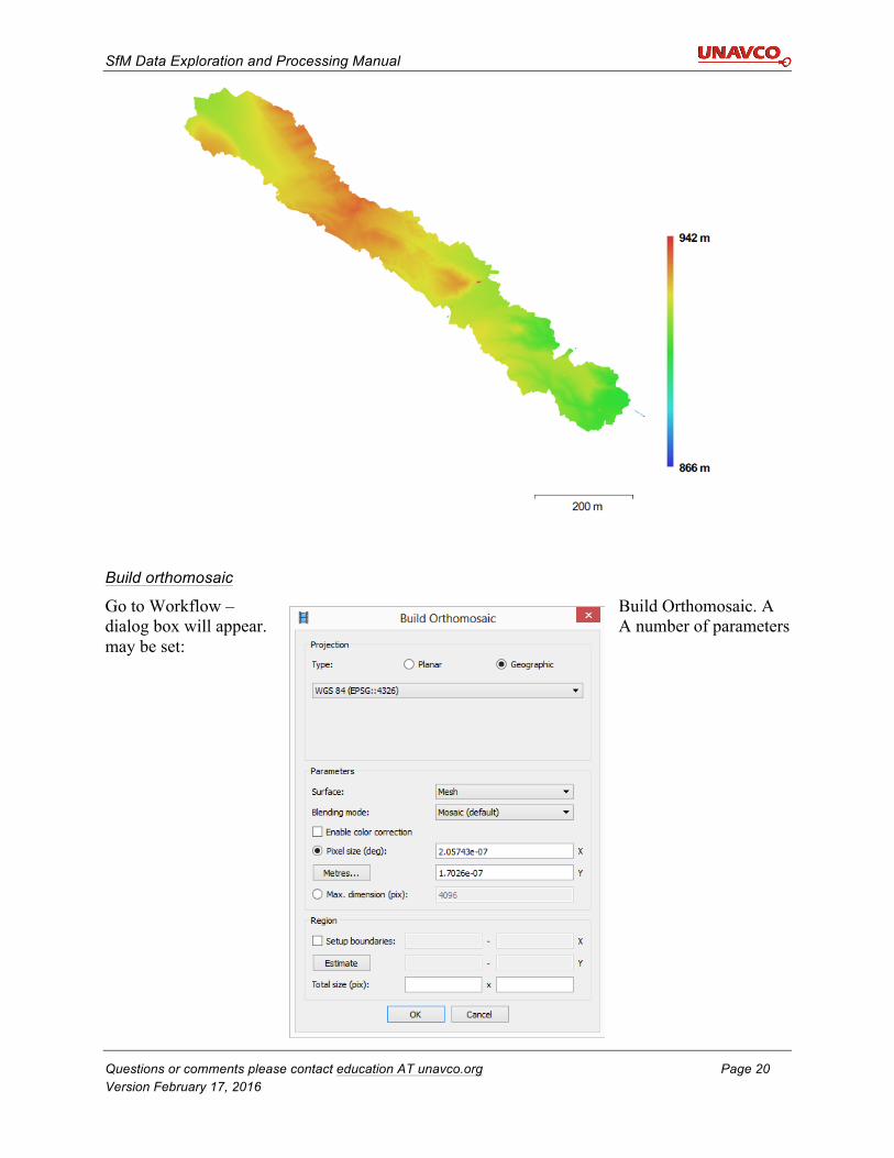
Build orthomosaic

Go to Workflow – Build Orthomosaic. A dialog box will appear. A number of parameters may be set:



1. Surface: the source of the surface for texture overlay a. DEM: best for aerial survey data or other georeferenced data. b. Mesh: best for non-georeferenced data.

2. Blending mode: how the pixels from different photos of the same feature will be combined.

a. Mosaic: default, blends specific pixels from photo with best representation of feature with pixels from other images to avoid seams in the texture.

b. Average: averages all pixels from all photos containing that feature. c. Disabled: not blended, best photo of each feature is used for the coloration of that

point. 3. Enable color correction: use when the photoset has extreme brightness variation. 4. Pixel size: recommended pixel size based on the ground sampling resolution; do not

decrease. However, if needed to reduce file size, you may increase this value. 5. Max dimension (pix): Maximum dimension for the produced file.

Product below. *Note: this will produce an orthomosaic for the whole dataset, not just the data within the bounding box. Data will need to be deleted to produce a smaller orthomosaic.



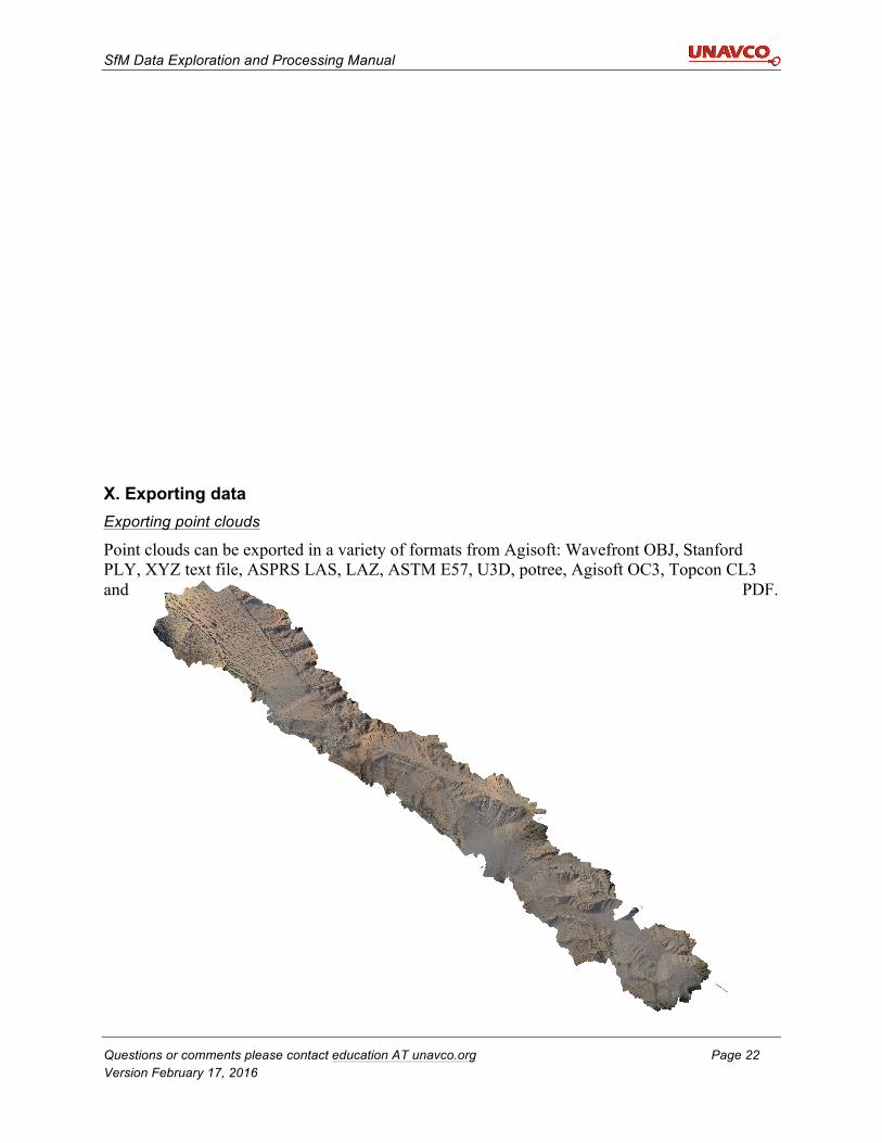
X. Exporting data Exporting point clouds

Point clouds can be exported in a variety of formats from Agisoft: Wavefront OBJ, Stanford PLY, XYZ text file, ASPRS LAS, LAZ, ASTM E57, U3D, potree, Agisoft OC3, Topcon CL3 and PDF.



Recommended file formats are LAS, LAZ, and XYZ as they work with the vast majority of point cloud viewing programs and allow for color data to be associated with each point.

Go to File – Export Points. Choose the file type, type of point cloud, and coordinate system. Exporting DEMs

Go to File – Export DEM – Export GeoTIFF/BIL/XYZ. A number of parameters may be set:

1. Coordinate system: you may choose a different coordinate system than the one GCPs were recorded in; you may also choose to do this conversion in another program.

2. Pixel size: you may adjust pixel size to be smaller than the suggested value to increase the effective resolution or larger to decrease the file size.

3. Maximum dimension in pixels 4. Split into blocks: useful for extremely large datasets 5. No-data value: -9999 if the file is going to ArcGIS, NaN is useful for MATLAB. Base this

value on the application you use for post-processing. 6. Region: you may set boundaries for what is included in the export 7. Write KML/Write World: georeferencing information; not needed if GeoTIFF is the file

format. Write KML only works for WGS84 because that is the coordinate system Google Earth supports.

Exporting orthomosaic

Go to File – Export DEM – Export JPEG/TIFF/PNG.

1. Coordinate system: you may choose a different coordinate system than the one GCPs were recorded in

2. Pixel size: keep pixel size at the recommended pixel size or greater. 3. Split into blocks: useful for extremely large datasets 4. Region: you may set boundaries for what is included in the export. 5. Compression: specify the compression needed. The exported file will be very large, so it

may be necessary to use an iterative process to adjust the compression for your post-processing needs.



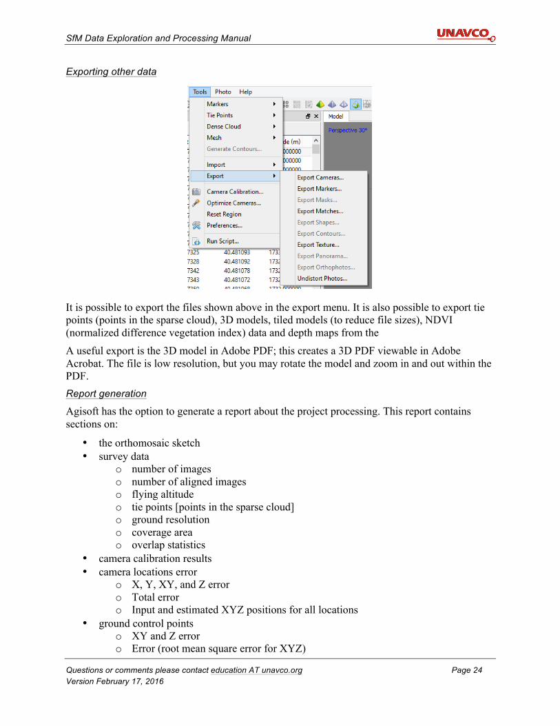
Exporting other data

It is possible to export the files shown above in the export menu. It is also possible to export tie points (points in the sparse cloud), 3D models, tiled models (to reduce file sizes), NDVI (normalized difference vegetation index) data and depth maps from the A useful export is the 3D model in Adobe PDF; this creates a 3D PDF viewable in Adobe Acrobat. The file is low resolution, but you may rotate the model and zoom in and out within the PDF. Report generation

Agisoft has the option to generate a report about the project processing. This report contains sections on:

• the orthomosaic sketch • survey data

o number of images o number of aligned images o flying altitude o tie points [points in the sparse cloud] o ground resolution o coverage area o overlap statistics

• camera calibration results • camera locations error

o X, Y, XY, and Z error o Total error o Input and estimated XYZ positions for all locations

• ground control points o XY and Z error o Error (root mean square error for XYZ)



o Projections o Total error

• DEM o Resolution o Point density

• Processing parameters o Input parameters for each step o Processing time

XI. Beyond the basics: additional useful information Chunks

Processing time in Agisoft increases significantly with increasing numbers of photos. As such, it is sometimes more efficient to split the photos into smaller portions, called chunks. The chunks can be individually processed and then merged at any step, though they are generally merged after the texture has been generated (i.e. the final step of processing). However, the Merge Chunks operation does not work optimally and may delete portions of the model or stitch the two chunks together inaccurately. If absolutely necessary to use chunks because of the number of photographs and the processing speed of your computer, the workflow below is the best to use:

• Align photos • Enter GCPs• Duplicate the chunk multiple times (good rule of thumb: take the number of photos,

divide by 250, and then duplicate the chunk that number of times). • Use the Resize Region tool to resize the bounding box in each duplicate chunk to 1/#

chunks in size. There should be some overlap between the edges of the bounding boxes to help align the chunks later.

• Then process each chunk separately for the dense cloud and the mesh steps. • Align the chunks. Merge the chunks. • Export the DEM/Orthomosaic.

Batch processing

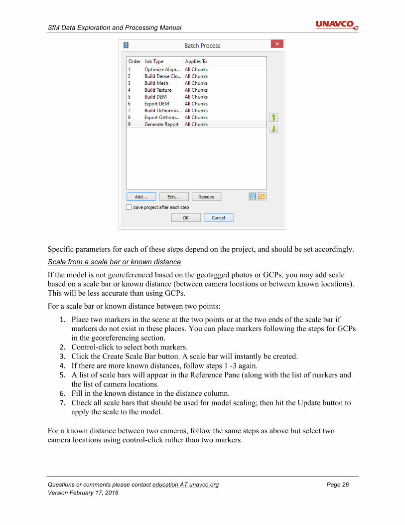
One of the most useful tools in Agisoft is the ability to batch process the data, so the workflow does not pause after every step. This also reduces the amount of hands-on time for the operator. To batch process the data, go to Workflow – Batch Process. Every automated step described in the above sections is available as a step in batch processing. To build a workflow, hit the Add button. A dialog box will appear with options to select the operation, select which chunks to apply the process, and input parameters for the operation. A suggested workflow is below.

• Align photosStart batch process here after identifying GCPs:



Specific parameters for each of these steps depend on the project, and should be set accordingly. Scale from a scale bar or known distance

If the model is not georeferenced based on the geotagged photos or GCPs, you may add scale based on a scale bar or known distance (between camera locations or between known locations). This will be less accurate than using GCPs. For a scale bar or known distance between two points:

1. Place two markers in the scene at the two points or at the two ends of the scale bar if markers do not exist in these places. You can place markers following the steps for GCPs in the georeferencing section.

2. Control-click to select both markers. 3. Click the Create Scale Bar button. A scale bar will instantly be created. 4. If there are more known distances, follow steps 1 -3 again. 5. A list of scale bars will appear in the Reference Pane (along with the list of markers and

the list of camera locations. 6. Fill in the known distance in the distance column. 7. Check all scale bars that should be used for model scaling; then hit the Update button to

apply the scale to the model.

For a known distance between two cameras, follow the same steps as above but select two camera locations using control-click rather than two markers.



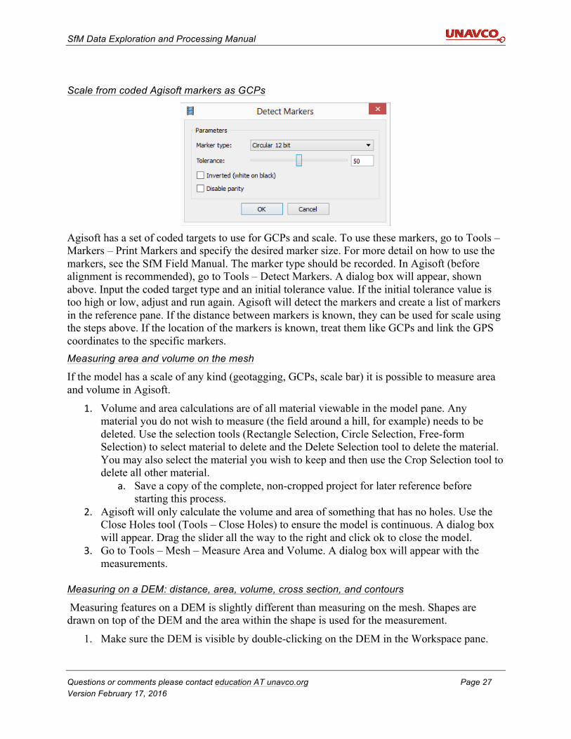
Scale from coded Agisoft markers as GCPs

Agisoft has a set of coded targets to use for GCPs and scale. To use these markers, go to Tools – Markers – Print Markers and specify the desired marker size. For more detail on how to use the markers, see the SfM Field Manual. The marker type should be recorded. In Agisoft (before alignment is recommended), go to Tools – Detect Markers. A dialog box will appear, shown above. Input the coded target type and an initial tolerance value. If the initial tolerance value is too high or low, adjust and run again. Agisoft will detect the markers and create a list of markers in the reference pane. If the distance between markers is known, they can be used for scale using the steps above. If the location of the markers is known, treat them like GCPs and link the GPS coordinates to the specific markers. Measuring area and volume on the mesh

If the model has a scale of any kind (geotagging, GCPs, scale bar) it is possible to measure area and volume in Agisoft.

1. Volume and area calculations are of all material viewable in the model pane. Any material you do not wish to measure (the field around a hill, for example) needs to be deleted. Use the selection tools (Rectangle Selection, Circle Selection, Free-form Selection) to select material to delete and the Delete Selection tool to delete the material. You may also select the material you wish to keep and then use the Crop Selection tool to delete all other material.

a. Save a copy of the complete, non-cropped project for later reference before starting this process.

2. Agisoft will only calculate the volume and area of something that has no holes. Use the Close Holes tool (Tools – Close Holes) to ensure the model is continuous. A dialog box will appear. Drag the slider all the way to the right and click ok to close the model.

3. Go to Tools – Mesh – Measure Area and Volume. A dialog box will appear with the measurements.

Measuring on a DEM: distance, area, volume, cross section, and contours

Measuring features on a DEM is slightly different than measuring on the mesh. Shapes are drawn on top of the DEM and the area within the shape is used for the measurement.

1. Make sure the DEM is visible by double-clicking on the DEM in the Workspace pane.



2. You can Draw Point, Draw Polyline, or Draw Polygon using the different tool buttons in the toolbar.

a. To finish a Polyline, double click. b. To finish a Polygon, put the last point on top of the first point. c. Finished shapes will appear in the workspace pane. d. To edit a point, line or polygon, double click the shape in the workspace pane.

This will bring up the Vertex Context menu. From here, you can delete the vertex or insert a vertex.

3. Measure a point coordinate: hold the cursor over the Point. The height of the point, as well as its X-Y coordinates, will appear.

4. Measure distance: right-click a Polyline; select Measure from the dropdown menu that appears. The value in the Perimeter box in the dialog box that appears should be the appropriate distance

5. Measure area and volume: right-click a Polygon; select Measure from the dropdown menu that appears. The value on the Planar tab is the area and the value on the volume tab is the volume.

6. Calculate a cross section: a. Create the line of section by making a Polyline. b. Right-click the Polyline and select Measure from the dropdown menu. c. Go to the Profile tab to see the cross section.

7. Create contours: Go to Tools – Generate Contours. A dialog box will appear. A number of parameters may be set:

a. Source data: DEM b. Minimal altitude c. Maximal altitude d. Interval

Contours can be show over a DEM or orthomosaic. Contours can also be exported from the Tools menu.

Bounding box alignment

The bounding box is set at an arbitrary orientation. On occasion, it is useful to modify the orientation of the bounding box to a specific reference frame. An example python script to do this is here: https://github.com/geojames/photoscan. This can be run from the command line or within Agisoft (Tools – Run Script). Python scripts

Agisoft has provided a number of Python scripts to perform additional tasks on their wiki page: http://wiki.agisoft.com/wiki/Python . This includes scripts to change the bounding box orientation (like above), to change the coordinate system to the bounding box, copy the bounding box orientation, batch export orthophotos, create masks based on specific colors, and automatically splitting data into chunks after photos are aligned and then merging chunks after the dense cloud and mesh have been built.

sfm data processing exploration v3 - UNAVCO

Documents

Transcript of sfm data processing exploration v3 - UNAVCO