arX

iv:0

807.

4129

v1 [

hep-

ph]

25

Jul 2

008

SFB/CPP-08-53TTP08-32

Feynman Integral Evaluation by a Sector

decomposiTion Approach (FIESTA)

A.V. Smirnov a,b, M.N. Tentyukov b

a Scientific Research Computing Center - Moscow State University, 119991Moscow, Russia

b Institut fur Theoretische Teilchenphysik - Universitat Karlsruhe, 76128Karlsruhe, Germany

Abstract

Up to the moment there are two known algorithms of sector decomposition: anoriginal private algorithm of Binoth and Heinrich and an algorithm made publiclast year by Bogner and Weinzierl. We present a new program performing the sectordecomposition and integrating the expression afterwards. The program takes a setof propagators and a set of indices as input and returns the epsilon-expansion ofthe corresponding integral.

PACS: 02.60.Jh; 02.70.Wz; 11.10.Gh.

Key words: Feynman diagrams; Sector decomposition; Numerical integration;Data-driven evaluation.

PROGRAM SUMMARY

Manuscript Title: Feynman integral evaluation by a sector decomposition approachAuthors: A.V. Smirnov, M.N. TentyukovProgram Title: FIESTAJournal Reference:Catalogue identifier:Licensing provisions: GPLv2Programming language: Wolfram Mathematica 6.0 and CComputer: from a desktop PC to a supercomputerOperating system: Unix, WindowsRAM: depends on the complexity of the problemNumber of processors used: the program can successfully work with a single proces-sor, however it is ready to work in a parallel environment, and the use of multi-kernelprocessor and multi-processor computers significantly speeds up the calculation

Preprint submitted to Elsevier 25 July 2008

Keywords: Feynman diagrams; Sector decomposition; Numerical integration; Data-driven evaluation.PACS: 02.60.Jh; 02.70.Wz; 11.10.Gh.Classification: 4.4 Feynman diagrams, 4.12 Other Numerical Methods, 5 ComputerAlgebra, 6.5 Software including Parallel AlgorithmsExternal routines/libraries: QLink [1], Vegas [2]Nature of problem: The sector decomposition approach to evaluating Feynman in-tegrals falls apart into the sector decomposition itself, where one has to minimizethe number of sectors; the pole resolution and epsilon expansion; and the numericalintegration of the resulting expressionSolution method: The sector decomposition is based on a new strategy. The sec-tor decomposition, pole resolution and epsilon-expansion are performed in Wolfram

Mathematica 6.0 [3]. The data is stored on hard disk via a special program, QLink[1]. The expression for integration is passed to the C-part of the code, that parsesthe string and performs the integration by the Vegas algorithm [2]. This part of theevaluation is perfectly parallelized on multi-kernel computers.Restrictions: The complexity of the problem is mostly restricted by CPU time re-quired to perform the evaluation of the integral, however there is currently a limitof maximum 11 positive indices in the integral; this restriction is to be removed infuture versions of the code.Running time: depends on the complexity of the problemReferences:

[1] http://qlink08.sourceforge.net, open source

[2] G. P. Lepage, the Cornell preprint CLNS-80/447,1980.

[3] http://www.wolfram.com/products/mathematica/index.html

2

LONG WRITE-UP

1 Introduction

Sector decomposition in alpha (Feynman) parametric representations of Feyn-man integrals originated as a tool for analyzing the convergence and provingtheorems on renormalization and asymptotic expansions of Feynman integrals[1]. The goal of this procedure is to decompose the initial integration domaininto appropriate subdomains (sectors) and introduce, in each sector, new vari-ables in such a way that the integrand factorizes, i.e. becomes equal to amonomial in new variables times a non-singular function. General mathemati-cal results on Feynman integrals exist up to now only in the case where all theexternal momenta are Euclidean. However, in practice, one often deals withFeynman integrals on a mass shell or at threshold.

Sector decomposition became a practical tool for evaluating Feynman integralsnumerically with the growth of computer power. Practical sector decomposi-tion was introduced in [2] and was used to verify several analytical results formultiloop Feynman integrals, including three-loop [3,4,5] results. For a goodreview on the sector decomposition we refer to Ref. [6].

The first public algorithm has been published by Bogner and Weinzierl [7].It proposes four strategies for the sector decomposition; three of those areguaranteed to terminate. Strategy A [8] is conceptually the simplest, howeverit results in too many sectors; strategy B (Spivakovsky’s strategy) has beendescribed in [9], strategy C has been created by Bogner and Weinzierl and isan improvement of strategy B. Strategy X is likely to share the ideas of Binothand Heinrich [2] It is not guaranteed to terminate but results in less sectors,than the other strategies.

This paper presents a new algorithm FIESTA for evaluating Feynman integralswith the use of sector decomposition. We reproduced the strategies A, B andX in the code and presented a new strategy S, based on original ideas. Ourstrategy is also guaranteed to terminate, but results in more sectors thanstrategy X, however the difference is between S and X is not so significantas with B and X. We provide an example where the strategy X does notterminate. For details and the table comparing the various strategies pleaserefer to Appendix A.

Our algorithm can successfully work with a single processor, however it isready to work in a parallel environment, and the use of multi-kernel processorsand multi-processor computers significantly speeds up the calculation.

3

To benchmark the power of FIESTA, we evaluated the triple box diagram [3](which starts from ε−6 poles) up to the finite part. We used the strategyX and took the symmetries of the diagram into account (see section 6 forthe syntax). A Xeon double processor computer was used (8 cores Intel(R)Xeon(R) CPU E5472, 3.00GHz, 1600FSB, 2x6MB L2 cache, 32 GB RAM,4.6TB local hard drive). The evaluation took less than 3 days (62.4 hours);the job used maximally 1GB of RAM and 40GB on hard drive. All the answersare within the 1 percent error estimate from the existing analytical result.

We tested FIESTA only on Windows and Linux platforms but there are noLinux-specifics; it should be possible to compile the sources on any Unix plat-form. However, we provide the pre-compiled binary files only for Windows onx86 and Linux on x86-64.

2 Theoretical background

FIESTA calculates Feynman integrals with the sector decomposition approach.It is based on the α-representation of Feynman integrals. After performingDirac and Lorentz algebra one is left with a scalar dimensionally regularizedFeynman integral [10]

F (a1, . . . , an) =∫

· · ·∫

ddk1 . . .ddkl

Ea11 . . . Ean

n

, (1)

where d = 4 − 2ε is the space-time dimension, an are indices, l is the numberof loops and 1/En are propagators. We work in Minkowski space where thestandard propagators are the form 1/(−p2 + m2 − i0). Other propagators arepermitted, for example, 1/(v · k± i0) may appear in diagrams contributing tostatic quark potentials or in HQET where v is the quark velocity. Substituting

1

Eaii

=eaiπ/2

Γ(a)

∞∫

0

dααai−1e−iEiα, (2)

changing the integration order, performing the integration over loop momenta,replacing αi with xiη and integrating over η one arrives at the following formula(see e.g. [11]):

F (a1, . . . , an) =

Γ(A − ld/2)∏n

j=1 Γ(aj)

∫

xj≥0

dxi . . . dxnδ

(

1 −n∑

i=1

xi

)

n∏

j=1

xaj−1j

UA−(l+1)d/2

F A−ld/2, (3)

4

where A =∑n

i=1 an and U and F are constructively defined polynomials of xi.The formula (3) has no sense if some of the indices are non-positive integers,so in case of those the integration is performed according to the rule

∞∫

0

dxx(a−1)

Γ(a)f(x) = f (n)(0)

where a is a non-positive integer.

After performing the decomposition of the integration region into the so-calledprimary sectors [2] and making a variable replacement, one results in a linearcombination of integrals of the following form:

1∫

xj=0

dxi . . . dxn′

n′

∏

j=1

xaj−1j

UA−(l+1)d/2

F A−ld/2(4)

If the functions UA−(l+1)d/2

F A−ld/2 had no singularities in ε, one would be able to per-form the expansion in ε and perform the numerical integration afterwards.However, in general one has to resolve the singularities first, which is not pos-sible for general U and F . Thus, one starts a process the sector decompositionaiming to end with a sum of similar expressions, but with new functions U andF which have no singularities (all the singularities are now due to the part∏n

j=1 x′a′

j−1

j ). Obviously it is a good idea to make the sector decompositionprocess constructive and to end with a minimally possible number of sectors.The way sector decomposition is performed is called a sector decomposition

strategy and is an essential part of the algorithm.

After performing the sector decomposition one can resolve the singularities byevaluating the first terms of the Taylor series: in those terms one integrationis taken analytically, and the remainder has no singularities. Afterwards theε-expansion can be performed and finally one can do the numerical integrationand return the result.

Please keep in mind that this approach works only using numerical integration:the values for all invariants should be substituted at the very early stage, aftergenerating the functions U and F .

3 Overview of the software structure

FIESTA is written in Wolfram Mathematica 6.0 and C. The user is not sup-

5

posed to use the C part directly as it is launched from Mathematica via theMathlink protocol. The C part is performing the numerical integration withthe use of the Vegas [13,14] algorithm implemented as a FORTRAN program.The Mathematica part can work independently, however the C-integration ismuch more powerful than the Mathematica built-in one. Hence to calculatecomplicated integrals one should use the C-integration.

4 Description of the individual software components

The Mathematica part is a .m file that is loaded into Mathematica simply by<<FIESTA 1.0.0.m 1 .

The Mathematica part of the program takes as input the set of loop momenta,the set of propagators, the set of indices and the required order of ε-expansionto be evaluated. It performs the differentiation (in case of negative indices),the sector decomposition, the resolution of singularities, the ε-expansion andprepares the expressions for the numerical integration. The numerical integra-tion can both be performed by Mathematica or by the C-part of FIESTA. TheMathematica integration has the advantage of being able to work with com-plex numbers (in future version this feature will also be added to the C-part),however, the C-integration is much more powerful and should be used if onegoes for complicated integrals.

The C-integration is called from Mathematica via the Mathlink protocol. Thispart of the algorithm can perfectly work in a parallel environment: one sim-ply has to specify the number of copies of CIntegrate to be launched. TheMathematica part distributes the integration tasks between those copies andcollects the result, preparing the expression of the next order at the same time.

The C-integration comes as a set of source files and should be compiled first.The binary files of CIntegrate for Linux and Windows can be downloadedfrom the web-page of the projecthttp://www-ttp.particle.uni-karlsruhe.de/∼asmirnov/FIESTA!.htm

The C-integration is using Vegas [13,14] to perform the integration. It takesa string with the expression from Mathematica as input, and performs aninternal compilation of this string to be able to evaluate the expression fastafterwards. No external compiler is required and no files are used for dataexchange.

In complicated cases one should use the QLink program [15] to store intermedi-

1 The paths to the CIntegrate binary, to the QLink[15] and the database shouldbe specified beforehand; see section 5 for details.

6

atedata from Mathematica on disk instead of RAM. QLink can be downloadedas a binary or as a source (it comes under the terms of GNU GPLv2).

5 Installation instructions

In order to install FIESTA, the user has to download the installation packagefrom the following URL:http://www-ttp.particle.uni-karlsruhe.de/∼asmirnov/data/FIESTA.tar.gz,unpack it and follow the instructions in the file INSTALL.

The Mathematica part of FIESTA requires almost no installation, one onlyneeds to copy the FIESTA 1.0.0.m file and edit the default paths QLinkPath,CIntegratePath and DataPath in this file, e.g.:

• QLinkPath="/home/user/QLink/QLink";• CIntegratePath="/home/user/FIESTA/CIntegrate";• DataPath="/tmp/user/temp";

Here QLinkPath is a path to the executable QLink file, CIntegratePath isa path to the executable CIntegrate file, and DataPath is a path to thedatabase directory. For the Windows system, these paths should look like

• QLinkPath="C:/programs/QLink/QLink.exe" 2 ;• CIntegratePath="C:/programs/FIESTA/CIntegrate.exe";• DataPath="D:/temp";

Note, the program will create a big IO traffic to the directory DataPath, thusit is better to put this directory on a fast local disk.

Alternatively, one can specify all these paths manually after loading the fileFIESTA 1.0.0.m into Mathematica.

Please note that the code requires Wolfram Mathematica 6.0 to be installedand will not work correctly under lower versions of Mathematica.

In order to work with nontrivial integrals, the user must install QLink andthe C-part of FIESTA, the CIntegrate program. The QLink [15] can be down-loaded as a binary file or compiled from the sources. If the user decides to usepre-compiled CIntegrate executable file, he has to place the file to some lo-cation and edit the paths in the file FIESTA 1.0.0.m as it is described above.If the user wants to compile the executable file himself he must have theMathematica Developer Kit installed on his computer.

2 Mathematica uses normal slashes for paths both in Unix and Windows.

7

Under Unix, the user must edit the file comdef.h to be sure that the macroWIN is not defined, i.e., comment the macrodefinition #define WIN 1. Thenthe self-explanatory file Makefile can be used by means of running the “make”command (the path to the Mathematica Developer Kit libraries should beprovided). As a result, the binary file CIntegrate appears.

For the Windows installation, the user must edit the file comdef.h to ensurethat the macro WIN is defined, #define WIN 1. The Windows makefile isprovided in the package; it is named “CIntegrate.mak” and is used with the“nmake /f CIntegrate.mak”; To run this command one has to have the Mi-crosoft Visual C++ installed (an express edition of Microsoft Visual C++ canbe downloaded for free from the Microsoft site). As an addition to the pro-grams and packages mentioned above, the user should install the MicrosoftPlatform Software Developer Kit (It can also be downloaded freely after vali-dating a genuine copy of Microsoft Windows) and the Intel Fortran compiler(an evaluation copy is also available form the Intel site).

6 Test run description

To run FIESTA load the FIESTA 1.0.0.m into Wolfram Mathematica 6.0. Toevaluate a Feynman integral one has to use the command

SDEvaluate[{U,F,l},indices,order],

where U and F are the functions from formula (3), l is the number of loops,indices is the set of indices and order is the required order of the ε-expansion.

To avoid manual construction of U and F one can use a build-in function UF

and launch the evaluation as

SDEvaluate[UF[loop momenta,propagators,subst],indices,order],

where subst is a set of substitutions for external momenta, masses and othervalues (note, the code performs numerical integrations. Thus the functions U

and F should not depend on any external values).

Example:

SDEvaluate[UF[{k},{-k2,-(k+p1)2,-(k+p1+p2)

2,-(k+p1+p2+p4)2},

{p21 →0,p2

2 →0,p24 →0, p1 p2 →-S/2,p2 p4 →-T/2,p1 p4 →(S+T)/2,

S→3,T→ 1}], {1,1,1,1},0]

performs the evaluation of the massless on-shell box diagram (Fig. 1) wherethe Maldestam variables are equal to S = 3 and T = 1. A complete log of this

8

example follows in Appendix B.

p4p2 3

2 4

p3p1 1

Fig. 1. The massless on-shell box diagram.

To clear the results from memory use the ClearResults[] command.

The code has the following options:

• UsingC: specifies whether the C-integration should be used; default value:True;

• CIntegratePath: path to the CIntegrate binary;• NumberOfLinks: number of the CIntegrate programs to be launched; de-

fault value: 1;• UsingQLink: specifies whether QLink should be used to store data on disk;

works only with UsingC=True; default value: True; please refer to Ap-pendix D on the use of QLink;

• QLinkPath: path to the QLink binary;• DataPath: path to the place where QLink stores the data; for example,

if DataPath=/temp/temp, then the code three directories: /temp/temp1,/temp/temp2 and /temp/temp3; those directories will be erased if existent;the directory /temp should exist;

• PrepareStringsWhileIntegrating: specifies whether the code should pre-pare expressions of next order in epsilon at the same time with integrating;works only with UsingC=True and UsingQLink=True; should be set to Falseon slow machines; default value: True;

• IntegrationCut: the actual low boundary of the integration domain (in-stead of zero); default value: 0;

• IfCut and VarExpansionDegree: if IfCut is nonzero then the expressionis expanded up to order VarExpansionDegree over some of the integrationvariables; the integration function is evaluated exactly if the integrationvariable is greater that IfCut, otherwise the expansion is taken instead; thedefault value of IfCut is zero, the default value of VarExpansionDegree is1;

• ForceMixingOfSectors: if set to True, forces the code to perform one in-tegration only for a given order of ε; default value is False; please refer toAppendix G;

9

• PrimarySectorCoefficients: The usage of this option allows to take thesymmetries of the diagram into account. If the diagram has symmetries,then the primary sectors corresponding to symmetrical lines result in equalcontributions to the integration result. Hence it makes sense to speed upthe calculation by specifying the coefficients before the primary sector in-tegrands. For example, if two lines in the diagram are symmetrical, onecan have a zero coefficient before one of those and 2 before the second.PrimarySectorCoefficients defines those coefficients if set; the size ofthis list should be equal to the number of primary sectors;

• STRATEGY: defines which sector decomposition strategy is used; STRATEGY 0

is not exactly a strategy, but an instruction not to perform the sector decom-position; STRATEGY A and STRATEGY B are the two strategies from Ref. [7]guaranteed to terminate; STRATEGY S (default value) is our strategy, pro-ducing better results than the preceding ones; STRATEGY X is an heuristicstrategy from [7]; likely to share the ideas of Binoth and Heinrich [2]: pow-erful but not guaranteed to terminate;

• ResolveNegativeTerms: defines whether an attempt to get rid of negativeterms in F should be performed; default value: True; see Appendix C;

• VegasSettings: a list of 4 numbers {p1, r1, p2, r2}, instructs the code toevaluate the integral r1 times with p1 sampling points for warm-up andr2 times with p2 sampling points for the final integration; default value:{10000, 5, 100000, 15}.

The code sometimes returns Indeterminate as a result. There are the follow-ing reasons possible:

• Negative function F provided ;This might happen if the propagators in the input for UF are of the form

−1/(−p2 + m2 − i0) instead of 1/(−p2 + m2 − i0);Solution: change the sign of the propagators;

• Complex number as an answer ;If the integrand has complex values, then the C integration cannot be

used with the current version of FIESTA. If complex numbers are explicitlyencountered in the integrand, the integration will produce a syntax error.Otherwise, if the expressions like log(−1) are encountered in the integrand,it the integration program returns Indeterminate;

Solution: One can try to use the UsingC=False option, however the built-in Mathematica integration cannot work in complicated examples and wedon’t guarantee correct results if complex numbers are used. The supportfor complex numbers will be provided in future versions of FIESTA;

• Special singularities;The standard sector decomposition approach works only for singularities

for small values of variables. Our code can resolve some extra singulari-ties (see Appendix C), but surely all types of singularities could not be becovered.

10

Solution: One can try different values of the ResolveNegativeTerms op-tion. If the singularity is of a special type, one can try contact the authorsin order to try to make the resolution of singularities of this type automatic.

• Numerical instability ;If all the singularities are for small values of integration variables, they

are resolved in the code. However, the numerical integration may experienceproblems with small values of variables (see Appendix E).

Solution: One should use the IntegrationCut or IfCut together withVarExpansionDegree options. See Appendix E for details.

7 Acknowledgements

The authors would like to thank V.A. Smirnov and M. Steinhauser for posingthe problem of sector decomposition and for testing in on various examples,to P. Uwer for the consultation on Vegas and numerical integration and toG. Heinrich for useful discussions.

This work was supported in part by DFG through SBF/TR 9 and RFBR08-02-01451-a.

Appendix

A Sector decomposition strategies

The sector decomposition goal may be reformulated the following way: sup-pose we have a polynomial P of n variables and a unitary hypercube U asintegration area. The task is to separate the integration region into a numberof sectors so that each of those sectors after a variable replacement turns intoa unitary cube and P in those variables turns into a product of a monomial Mand a polynomial of a proper form, i.e. having 1 as one of the summands. Thisrequirement is often sufficient for the polynomial P to have no zeros apartfrom the ones due to M (this is valid for a wide class of integrals includingthose with the same sign for all kinematic invariants).

The sector decomposition is usually performed recursively; for a given polyno-mial P one has an algorithm to define how to perform a single sector decom-position step. Such an algorithm is also called a sector decomposition strategy.

All known strategies separate U into parts the following way: a subset I =

11

{i1, . . . im} of {1, . . . , n} is chosen and m sectors are defined by

Sl = {(x1, . . . , xn) ∈ U|xil ≥ xik∀ik ∈ I},

(l = 1 . . .m). The variable replacement in Sl is defined by

xi = x′i ∀i 6∈ I

xil = x′il

xik = x′ilx′

ik∀i ∈ I, k 6= l

It is easy to verify that the integration region in the new variables x′ is againa unitary cube.

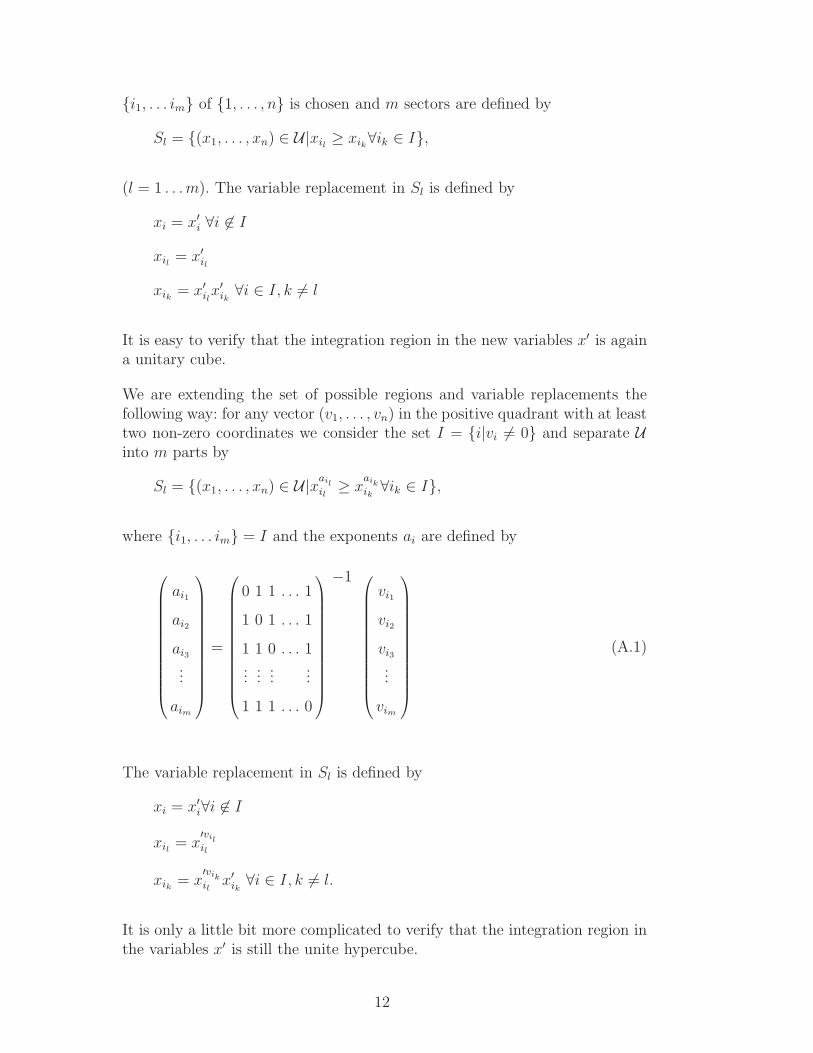
We are extending the set of possible regions and variable replacements thefollowing way: for any vector (v1, . . . , vn) in the positive quadrant with at leasttwo non-zero coordinates we consider the set I = {i|vi 6= 0} and separate Uinto m parts by

Sl = {(x1, . . . , xn) ∈ U|xailil

≥ xaikik

∀ik ∈ I},

where {i1, . . . im} = I and the exponents ai are defined by

ai1

ai2

ai3

...

aim

=

0 1 1 . . . 1

1 0 1 . . . 1

1 1 0 . . . 1...

......

...

1 1 1 . . . 0

−1

vi1

vi2

vi3

...

vim

(A.1)

The variable replacement in Sl is defined by

xi = x′i∀i 6∈ I

xil = x′vilil

xik = x′vikil

x′ik∀i ∈ I, k 6= l.

It is only a little bit more complicated to verify that the integration region inthe variables x′ is still the unite hypercube.

12

Now let us describe how we choose the vector v. We consider the set of weightsW of the polynomial P defined as the set of all possible (a1, . . . , an) wherecxa1

1 . . . xann is one of the monomials of P . We will say that a weight is higher

than another one if their difference is a set of non-negative numbers. If P hada unique lowest weight, a monomial could be factorized out and we would rep-resent P in the required form. Hence it becomes reasonable to try to minimizethe number of lowest weights of P . We consider the convex hull of W andchoose one of its facets F visible from the origin. Now v is chosen to be thenormal vector to F .

The reason of choosing such a vector is rather simple: the vectors formed bythe weights of the vectors x′

ikfor k 6= l are orthogonal to v, therefore are

lying in the facet F . Hence there is a good chance that after a single sectordecomposition step only one of the vertices of F is left to be a lowest weight.

Such a sector decomposition step is guaranteed not to increase the norm de-fined in the strategy A of [7] (the Zeillinger strategy [8]). If we can’t find afacet such that the corresponding step decreases the norm, we fall back to thestrategy A and perform one step. Hence our strategy is also guaranteed toterminate. Practice shows that the strategy A steps are applied in no morethan in five percent cases.

The following table shows the number of sectors produced by different strate-gies on various examples:

Diagram A B C S X

Box 12 12 12 12 12

Double box 755 586 586 362 293

Triple box M 114256 114256 22657 10155

D420 8898 564 564 180 F

D420 is a diagram contributing to the 2-loop static quark potential on Fig. A.1with the following set of propagators: {−k2,−(k − q)2,−l2,−(l − q)2,−(k −l)2,−vk,−vl}, where k and l are loop momenta, q2 = −1, qv = 0 and v2 = 1.

“F” means that the sector decomposition fails (we suppose an infinite loop).“M” means that the memory overflow happened during the sector decompo-sition on a 8Gb machine. We suspect D420 to be a counterexample to theSTRATEGY X

Hence we recommend leaving the default option STRATEGY=STRATEGY S (ourstrategy) or experimenting with STRATEGY=STRATEGY X (based on the ideas ofBinoth and Heinrich [2], not guaranteed to terminate).

13

Fig. A.1. A diagram contributing to the 2-loop static quark potential

B An example

Here we provide the listing of the Mathematica session for evaluation of themassless on-shell box diagram with S = 3 and T = 1 (we split some longlines).

In[1]:= << FIESTA_1.0.0.m

FIESTA, version 1.0.0

In[2]:= UsingQLink=False;

In[3]:= SDEvaluate[UF[{k},{-k^2,-(k+p1)^2,-(k+p1+p2)^2,

-(k+p1+p2+p4)^2},{p1^2->0,p2^2->0,p4^2->0,

p1 p2->-S/2,p2 p4->-T/2,p1 p4->(S+T)/2,S->3,

T->1}],{1,1,1,1},0]

External integration ready! Use CIntegrate to perform calls

FIESTA, version 1.0.0

UsingC: True

NumberOfLinks:1

UsingQLink: False

IntegrationCut: 0

IfCut: 0.

Strategy: STRATEGY_S

Integration has to be performed up to order 0

Sector decomposition..........0.0138 seconds; 12 sectors.

Variable substitution..........0.0055 seconds.

Decomposing ep-independent term..........0.0025 seconds

Pole resolution..........0.0081 seconds; 40 terms.

Expression construction..........0.0021 seconds.

Replacing variables..........0.0063 seconds.

Epsilon expansion..........0.0123 seconds.

Expanding..........0.0002 seconds.

Counting variables: 0.0002 seconds.

Preparing integration string..........0.0004 seconds.

Terms of order -2: 8 (1-fold integrals).

Numerical integration: 8 parts; 1 links;

Integrating..........0.106322 seconds; returned answer:

14

1.333333

Integration of order -2: 1.333333

(1.333333)/ep^2

Expanding..........0.0005 seconds.

Counting variables: 0.0005 seconds.

Preparing integration string..........0.001 seconds.

Terms of order -1: 28 (2-fold integrals).

Numerical integration: 12 parts; 1 links;

Integrating..........0.409080 seconds; returned answer:

-2.065743 +- 5.*^-6

Integration of order -1: -2.065743 +- 5.*^-6

(1.333333)/ep^2 + (-0.73241 +- 5.*^-6)/ep

Expanding..........0.0008 seconds.

Counting variables: 0.0009 seconds.

Preparing integration string..........0.0022 seconds.

Terms of order 0: 40 (2-fold integrals).

Numerical integration: 12 parts; 1 links;

Integrating..........0.862786 seconds; returned answer:

-3.417375 +- 0.000012

Integration of order 0: -3.417375 +- 0.000012

(1.333333)/ep^2 + (-0.73241 +- 5.*^-6)/ep +

(-4.386496 +- 0.000013)

Total time used: 1.52991 seconds.

-6

1.33333 -0.73241 + 5. 10 pm46

Out[3]= -4.3865 + ------- + -----------------------

2 ep

ep

+ 0.000013 pm47

In[4]:= Quit

The analytical answer for this integral is

4

3ε2−

2 log(3)

3ε−

4π2

9

which is equal to

1.33333331

ε2− 0.7324081

1

ε− 4.3864908.

C Dealing with negative terms in F

FIESTA has been used to verify master integrals for the three-loop static quark

15

potential [12]. A typical phenomenon when evaluating those integrals is thatthe function F can involve terms like (xi −xj)

2 = x2i −2xixj +x2

j . As a result,not all monomials of F have positive signs, resulting in extra singularities forthe integration.

To overcome those problems we added an additional feature to FIESTA: anattempt to get rid of negative summands in F before performing the sectordecomposition (those summands may lead to additional singularities that arenot treated properly by the basic approach). The code tries to find two vari-ables, xi and xj , split the unitary cube into two regions with xi ≤ xj andxi ≥ xj and do a variable replacement (e.g. for xi ≤ xj we make the replace-ment x′

i = xj − xi). In case of success, we result in a new function F withoutmonomials with negative sign.

The ideas of this type are not original; it is a common situation when certainclasses of integrals require a special treatment, in the papers of Binoth andHeinrich [2] one can find various examples where special operations preced-ing the sector decomposition are performed. Still we consider our automaticapproach to the problem to be original: one does not require to specify thesingularities of this type for the code to resolve them.

D Avoiding memory limits in Mathematica

Wolfram Mathematica, being a powerful CAS 3 is widely used among re-searchers nowadays. However, a significant drawback of the Mathematica us-age is the lack of RAM that is often encountered. FIESTA also had memoryproblems at the ε-expansion stage: an expression for a single sector can be-come huge after the expansion, and in complicated examples one can havemany thousands of sectors. To avoid memory problems we used the QLink

program to store data on hard disk.

After performing the sector decomposition we store all the expressions in adatabase via QLink. Afterwards the code never loads the whole set of expres-sions into RAM. On the contrary, the code works with sectors one by one:it loads an expression from the database, performs an operation with it andwrites it back to the database. The operation might be one of the following:singularity resolution, ε-expansion, applying the Expand function or applying“if conditions” (see appendix E).

It is worth noting that the ε-expansion does not use the Mathematica Series

function but explicit differentiation instead. This has two reasons: first of all,

3 Computer Algebra System

16

differentiation with subsequent expansion works faster in Mathematica 6.0for the expressions we consider (remember that FIESTA uses Mathematica

6.0 because of the powerful build-in integration methods that were absent in5.2). The second reason is to perform differentiation at the very beginningbut to wait with applying the Expand function (which takes more time thanthe differentiation!). The latter function can be applied simultaneously withthe integration at a later stage: we prepare expressions of order o + 1 whileintegrating expressions of order o.

Such an approach allows to keep the memory usage by Mathematica minimaland to leave most of the memory to the CIntegrate copies.

E Resolution of singularities and its influence on the convergenceof numerical integration

As it has been noted in section 2, the integrals

1∫

xj=0

dxi . . . dxn(n∏

j=1

xaj−1j )Z, (E.1)

where Z has no singularities might have singularities because of non-positiveaj . Let us assume that ai ≤ 0 and treat the integrand as a function xai−1Y (ai)with coefficients being polynomials of other variables. For readability we willomit the index i. We replace xa−1Y (a) by

Y (0)xa−1 + Y ′(0)xa + . . . +1

a!Y (−a)(0)x−1 +

xa−1(Y (a) − Y (0) − Y ′(0)x − . . . −1

a!Y (−a)(0))

The items in the first line of the expression can be analytically integratedover x leaving us with one integration less. As for the expression R(a) =xa−1(Y (a)−Y (0)−Y ′(0)x−. . .− 1

a!Y (−a)(0)), it is known to have no singularities

at x = 0, however it might result in numerical instabilities at a later stage.

After performing the resolution of singularities and the ε-expansion, one ob-tains a set of integrands depending only on integration variables over the unithypercube. The integrands arise from the expressions like R (or even morecomplicated ones in case of several integration variables).

Those integrands have no singularities, so one could expect that the integrationis performed with ease. However, one can see that for small x the xa−1 is huge

17

and the remainder is small. Hence the remainder can’t be evaluated exactlybecause it is a difference of not-so-small numbers stored with a finite numberof digits.

The first step to the solution is to expand the expressions before evaluating.It leaves similar problems (a difference of huge numbers resulting in a normalnumber), but with a smaller numerical instability. Still, in highly degener-ate examples the problem persists and prevents the code from evaluating thefunction when the variables turn small.

FIESTA has two methods to deal with the numerical instability. The firstmethod is the usage of the IntegrationCut option. This option sets the lowintegration limit to IntegrationCut (instead of zero). This approach maylead to high error estimate, so there is a more advanced method (slower butproviding better results).

The idea of the second method is to expand the integration function over theintegration variables around zero up to a certain order (not all integration vari-ables require the expansion, but only the ones with a negative exponent in thepreceding monomial). Then one can integrate the original function for valuesgreater than some fixed number and the expanded one for smaller values. Thecode is instructed to work this way by the IfCut and VarExpansionDegree

options. Please note that even for IfCut=10−2 and VarExpansionDegree=1

one results in an 10−6 relative error estimate for the remainder that is smallerthan the integration error estimate for complicated examples.

There is one more technical problem in the second approach: the usage ofthe Mathematica Series command can be quite slow. Hence to expand thefunction we need to substitute x = 0 into the function and its derivatives. Thedirect substitution is impossible for the same numerical reasons. The solutionscomes with finding the minimal possible s such that (xsf)(0) can be evaluated

numerically. Now we can define a new function g = (xsf)(s)

s!and use the fact

that f (l)(0) = C l+ss g(l)(0) to expand the function.

Please note that the error estimate in the output is the one that comes fromthe integration; if the cuts are used, one should keep in mind that the realerror might be greater for the reason that a function different from the originalone is integrated.

18

F External integration

F.1 Overview

For the integration we use the well-known Vegas algorithm [13,14] which isbased on importance sampling. It samples points from the probability distri-bution described by the function |f |, so that the points are concentrated inthe regions that make the largest contribution to the integral. In the presentversion of FIESTA we use the FORTRAN code linked with the C interface toMathematica. The VEGAS routine requires an integrand as a reference to afunction of an array of the integration variables x, the number of repetitionsand the number of sampling points.

The Mathematica part provides the integrand in a form of a long symbolicalgebraic expression consisting of the integration variables, powers and loga-rithm 4 , e.g.:

(1+x[1])*p[x[1]+x[1]*x[2],-3]+ l[x[3]]/33

where p[x[1]+x[1]*x[2],-3] stands for (x[1] + x[1] ∗ x[2])−3 and l[x[3]]

for log(x[3]).

The common approach is based on generating the corresponding C (or FOR-TRAN) code, compiling it, linking with some integration routine (VEGAS inour case), running the resulting program and reading back the answer. How-ever, in our case this approach does not work properly: it is specific to thesector decomposition that there can be many thousands of sectors. This leadsto a big overhead for loading a compiler, a linker, writing the results to a file,loading and starting the resulting program and reading the results back.

Next, the size of the corresponding expressions to be integrated may vary fromseveral bytes to hundreds of megabytes. Unfortunately, all of the existing C orFORTRAN compilers are strongly nonlinear with respect to the length of theinput expression. The reason is that these compilers usually use the so-calledAST (Abstract Syntax Tree, see [16]) which is a tree representation of thesyntax: each node represents constants or variables (leaves) and operators orstatements (inner nodes). The complexity of this tree grows rapidly with thesize of the incoming expression. In practice, it is nearly impossible to compilean expression of more then a few megabytes length.

In order to compile a huge expression one can use some stack-based program-

4 For the IfCut method (see Appendix E) the if-then-else construction is alsoused, in the form if(condition)(first branch)(second branch).

19

ming language like FORTH [17] but the performance of programs written onthese languages is usually not so good as the performance of C or FORTRANprograms.

One of the standard approaches consists in optimizing the algebraic expres-sion by means of some CAS tool like the Maple package “CodeGeneration”(formerly “codegen”)[18] and compiling the resulting C (or FORTRAN) codewithout optimization. This cannot solve our problem since the number of ex-pressions is too big, anyway, and the resulting (optimized) code sometimes isstill rather large. Moreover, the time the CAS spends to generate such an op-timized code is too large. So we decided to develop an interpreter which is ableto evaluate a given expression in a “data-driven” manner: a translator trans-lates the incoming expression into some internal representation 5 and then aninterpreter evaluates the expression many times for various input data. It isworth noting that no intermediate AST is generated, only the linear sequenceof triples. This permits our translator to be almost linear w.r.t. the length ofthe incoming expression.

F.2 Translation

The incoming expression consists of (many) terms. Each term is a productof a coefficient and a number of integration variables (possibly zero) in somepowers, some prescribed functions of these variables and subexpressions of thesame structure (recursively). The translator converts this expression into a se-quence of triples, being “an operation”, “first operand” and “second operand”;e.g. the expression 1+x[1]+x[1]*x[3] will be represented as a following se-quence of triples:

1: ’+’, 1, x[1]

2: ’*’, x[1], x[3]

3: ’+’, ^1, ^2

where ˆ1 is a reference to the result of the first triple evaluation, ˆ2 to thesecond one. A term may involve some functions and subexpressions, e.g.x[1]+p[x[1],-2]*(x[2]+x[3]) will be translated to

1: ’p’, x[1], -2

2: ’+’, x[2], x[3]

3: ’*’, ^1, ^2

4: ’+’, x[1], ^3

5 We use the triple form, see [16].

20

During translation, the subexpression optimization is performed in the fol-lowing way: the translator searches for each new triple in the dictionary. Ifthe triple has already occurred, the translator does not put the triple into theresulting sequence, referencing the old one instead. Note, the translator inputis already sorted since we get it from Mathematica so at least all coincidingmonomials will be evaluated only once.

This simple prefix optimization is surely not perfect. Let us consider the fol-lowing expression:

(1+x[1]+x[2]*x[4])*(1+x[2]*x[4]+x[2]*x[3]*x[4])

The terms are sorted but the subexpressions 1+x[2]*x[4] in brackets will notbe recognized, and x[2]*x[4] in x[2]*x[3]*x[4] also will not be identified.Of course, we might have implemented all possible combinations, but theresulting time would grow factorially w.r.t. the length of the input string,which is unacceptable for us. Hence we implemented the following strategy:

Let us consider a term. Let us assume it has an implicit coefficient 1 infront. We consider every factor as a “commuting diad” of a form “opera-tion”, “operand”, e.g. 3*x[1]*x[3]/x[2] will be considered as a set of thefollowing commuting diads:

’*’, 3

’*’, x[1]

’*’, x[3]

’/’, x[2]

Now we can re-order all these diads without affecting the result. We try toevaluate such a sequence in some “native” order, e.g. in the above examplethis would be like the following:

’*’, x[1]

’/’, x[2]

’*’, x[3]

’*’, 3

We put the coefficient to the end, so terms differing by a coefficient willbe evaluated only once. It is also worth noting that in each subexpressionMathematica already sums up all similar terms.

The same idea works out (even better) for summands, the only difference isthe implicit initial value 0 instead of 1.

This works well, reducing the number of generated triples by an order ofmagnitude. The translation procedure is in the worst case quadratic w.r.t. to

21

the length of the input string, in average it is a bit worse than linear. Typically,in a 3GHz Xeon processor the translator spends about 30 seconds to translatea gigabyte expression, which is incomparably less than the integration time.

F.3 Evaluation

The sequence of the translated triples is completely platform independent,and it is rather straightforward to generate (directly to the memory) the bi-nary executable code for any existing architecture, and execute it. For themoment, we’ve restricted ourselves by developing the interpreter suitable forevery platform.

First of all, the triple sequence we have from the translation stage, is trans-lated into the array of quadrples: “operation”, “operand 1”, “operand 2” and“result”. The fields “operand 1” and “operand 2” are pointers to some memoryaddresses. The “result” field is either the result of the quadruple evaluation(double type in C), or the address of the memory cell in which the resultmust be stored. The point is that the size of the address field on 64 bit plat-forms is the same as the size of double, and the usage of indirect referencesis rather slow, so it seems to be reasonable to use a new memory cell for eachintermediate result.

However, on a modern CPU such an approach appears to be completely wrong.Modern processors have a big write-back cache memory (megabytes), andprovided the same memory address is permanently updated it is never writtento RAM but stays in the cache. On the other hand, if we write intermediateresults every time to a new address, all this data is sooner or later writtento RAM (after the cache exhausted). That is why for “small” jobs, when allintermediate results fit into the processor cache, the interpreter stores resultsdirectly to the “result” field of a quadruple, while for “large-scale” jobs thetranslator creates some buffers and provides the quadruples with re-usableaddresses of elements of these buffers.

The algorithm switches from the “small” to “large” model when the numberof generated triples reaches some threshold which strongly depends on the sizeof the processor L2 (L3) cache per active core and it is a subject for tuningfor every specific architecture. The corresponding value is hard-coded, it canbe changed in the file scanner.h, the macroINDIRECT ADDRESSING THRESHOLD.

The complete structure of the C-part is as follows. The routine AddString()

builds the integrand step by step collecting the incoming lines. Every momentthe process may be canceled by invoking the function ClearString(). After(almost) all of the lines are collected, the routine Integrate() adds the rest

22

and invokes the translator. After the incoming expression is translated into thequadruple array the routine Integrate() invokes the VEGAS routine for 5repetitions with 10000 sampling points in order to “warmup” the grid. Finally,the VEGAS routine is invoked by the Integrate() routine for 15 repetitionswith 100000 sampling points for the real integration 6 .

G Integration of sums vs sums of integrations

The current version of FIESTA integrates in each sector separately (each sector,not just each primary sector). The results are summed up and the error esti-mate is calculated with a mean-square norm. This approach might encountera natural suspicion: the errors add up and might result in an absurd result.However practice shows that the real error of this method is normally onlyabout 20 percent greater that the error of the other approach — integratingthe sum of expressions.

The reason lies within the adaptable integration algorithms: if each of theterms is integrated individually, the algorithm can adapt to all the peaks ofthe given term. Hence the error estimate for the individual terms might begood enough. However when one tries to evaluate the whole sum at once, thepeaks and other peculiarities of the different terms collide and the integrationalgorithm cannot adapt to all of them properly.

Another reason to integrate in each sector individually is obviously the econ-omy of RAM. And even more, this approach suits well for parallel environ-ments due to much better load balancing.

For the CIntegrate interpreter short (but not so-short) expressions are alsopreferable.

At first sight, long expressions could be optimized much better than the shortones for the following reason: the longer the expression, the more commonsubexpressions are encountered, and all the subexpressions should be evalu-ated only once. But for a long expression the program must use the indirectreferencing for quadruple results (see Appendix F.3) which can slowdown theinterpreter considerably.

In general, all these effects speedup the evaluation up to an order of magnitudewhen each individual sector is integrated independently on others.

6 This is the default behavior; the exact number of sampling points can be set bythe VegasSettings option, see Section 6.

23

References

[1] N.N. Bogoliubov and O.S. Parasiuk, Izv. Akad. Nauk USSR 25 (1955) 429;N.N. Bogoliubov and D.V. Shirkov, Introduction to Theory of Quantized Fields,3rd edition, Wiley, New York, 1983;K. Hepp, Commun. Math. Phys., 2 (1966) 301;E.R. Speer, J. Math. Phys., 9 (1968) 1404;E.R. Speer, Ann. Inst. H. Poincare, 23 (1977) 1;P. Breitenlohner and D. Maison, Commun. Math. Phys., 52 (1977) 11, 39, 55;K. Pohlmeyer, J. Math. Phys., 23, (1982) 2511;V.A. Smirnov, Commun. Math. Phys., 134 (1990) 109;O.I. Zavialov, Renormalized Quantum Field Theory, Kluwer AcademicPublishers, Dodrecht, 1990;V.A. Smirnov, Applied Asymptotic Expansions in Momenta and Masses, STMP177, Springer, Berlin, Heidelberg, 2002.

[2] T. Binoth and G. Heinrich, Nucl. Phys. B, 585 (2000) 741 [hep-ph/0004013];T. Binoth and G. Heinrich, Nucl. Phys. B, 680 (2004) 375 [hep-ph/0305234];T. Binoth and G. Heinrich, Nucl. Phys. B, 693 (2004) 134 [hep-ph/0402265].

[3] V. A. Smirnov, Phys. Lett. B567 (2003) 193 [hep-ph/0305142].

[4] T. Gehrmann, G. Heinrich, T. Huber, C. Studerus, Phys. Lett. B640 (2006)252–259, [hep-ph/0607185].G. Heinrich, T. Huber and D. Maitre, Phys. Lett. B662 (2008) 344 [0711.3590].

[5] R. Boughezal and M. Czakon, Nucl. Phys. B755 (2006) 221, [hep-ph/0606232].T. Binoth and G. Heinrich, Nucl. Phys. B680 (2004) 375, [hep-ph/0305234].

[6] G. Heinrich, Int. J. of Modern Phys. A, 23 (2008) 10 [0803.4177];

[7] C. Bogner and S. Weinzierl, Comput. Phys. Commun., 178 (2008) 596[0709.4092].C. Bogner and S. Weinzierl, [0806.4307].

[8] D.Zeillinger, Enseign. Math. 52, 143 (2006).

[9] M. Spivakovsky, Progr. Math. 36, 419 (1983).

[10] G. ’t Hooft and M. Veltman, Nucl. Phys. B 44 (1972) 189;C.G. Bollini and J.J. Giambiagi, Nuovo Cim. 12 B (1972) 20.

[11] V.A. Smirnov, “Evaluating Feynman Integrals,” Springer Tracts Mod. Phys.211 (2004) 1;V.A. Smirnov, “Feynman integral calculus,” Berlin, Germany: Springer (2006)283 p.

[12] A.V. Smirnov, V.A. Smirnov and M. Steinhauser, PoS(ACAT) (2007) 024[0805.1871]A.V. Smirnov, V.A. Smirnov and M. Steinhauser, to appear in Nucl. Phys. B(Proc. Suppl.), [0807.0365]

24

[13] G. P. Lepage, J. Comp. Phys. 27, 192(1978).

[14] G. P. Lepage, the Cornell preprint CLNS-80/447,1980.

[15] QLink — open-source program by A.V. Smirnov, http://qlink08.sourceforge.net

[16] Alfred V. Aho et al., “Compilers: Principles, Techniques, and Tools (2ndEdition)”, Addison-Wesley, 2007.

[17] http://forthlinks.com

[18] K. Geddes et al., “Maple 9 Advanced Programming Guide”, Maplesoft, 2003,http://minerva.tau.ac.il/bsc/2/2130/docs/04/m9AdvancedProgrammingGuide.pdf,p. 319

25