Sewer asset management: impact of sample size and ...

Tim Maeckelberghe

decision-making multivariate modelcharacteristics on the calibration outcomes of aSewer asset management: impact of sample size and

Academic year 2013-2014Faculty of Engineering and ArchitectureChairman: Prof. Marc VanhaelstDepartment of Industrial Technology and Construction

Master of Science in de industriële wetenschappen: bouwkundeMaster's dissertation submitted in order to obtain the academic degree of

Supervisors: Prof. Patrick Ampe, dhr. Pascal Le Gauffre

PIRD - GCU/INSAL MAECKELBERGHE Tim June 2014

Gestion patrimoniale des réseaux d'assainissement: impact de l'échantillon sur la connaissance du patrimoine

Sewer asset management: impact of sample size and characteristics on the calibration outcomes of a decision-making multivariate model

Projet d’Initiation à la Recherche & Développement – juin 2014

MAECKELBERGHE Tim

Sous la direction de LE GAUFFRE Pascal

Département Génie Civil & Urbanisme

Laboratoire de Génie Civil et d'Ingénierie Environnementale (LGCIE)

20 Avenue A. Einstein, 69621 Villeurbanne Cedex, France

[email protected]

RÉSUMÉ. Plusieurs chercheurs ont développé des modèles de détérioration de la gestion patrimoniale des réseaux d'assainissement sans tenir compte de l'impact sur les résultats de l'échantillon choisi. Une étude précédente a investigué la représentativité de l'échantillon prélevé dans l'ensemble du patrimoine. Cette étude traitait de la meilleure technique d'échantillonnage et de la taille minimale de l'échantillon. L'impact de la taille des échantillons prélevés sur le modèle de régression logistique a été examiné en effectuant des tests d'analyse statistique. Ainsi, on a pu étudier les différences entre les échantillons et l'ensemble du patrimoine. L'étude a mené à plusieurs coefficients avec une valeur p supérieure à 10% pour les variables du modèle en fonction de la taille de l'échantillon.

La première partie de cet article est une suite à l'étude précédente et examine l'impact sur les résultats en éliminant des variables. Les échantillons qui ont une taille réduite mènent plutôt à des coefficients avec une valeur p supérieure à 10% des variables de la régression logistique, et peuvent être exclus. Des modèles différents dépendant de la corrélation des variables ont été investigués avec des méthodes d'échantillonnage et pour différentes tailles d'échantillons. La deuxième partie explique les effets des modifications sur le patrimoine qui sont mises en œuvre par la construction de nouveaux patrimoines virtuels afin d'arriver à des conclusions générales. Finalement quelques solutions pratiques sont proposées.

ABSTRACT. Many researchers have developed deterioration models for sewer asset management without paying attention to the impact of the chosen sample on the outcomes. Previous work has investigated the representativeness of the sample drawn out of the whole asset stock. The study tackled the best suited sampling technique and the minimum sample size. The impact of the sample size on the applied logistic regression model was investigated by performing statistical analysis tests. This way differences between the samples and the whole database were examined. The research led to various coefficients with a p value superior to 10% for variables of the model depending on the sampled size.

The first part of this paper builds on where the study left and investigates the impact on the outcome by eliminating variables. Smaller sample size leads to more coefficients with a p value superior to 10% of the variables of the logistic regression function, which can be excluded. Different models depending on the correlation of the variables are investigated with sampling techniques and for different sample sizes. The second part explains the consequences of changes in the applied database which are implemented by making virtual asset stocks, in order to draw general conclusions. As a result some practical solutions are proposed.

MOTS-CLÉS : gestion patrimoniale d'assainissement, régression logistique, analyse régression multi variable, méthodes d'échantillonnage.

KEYWORDS: sewer asset management, logistic regression, multivariable regression analysis, sampling techniques.


2

1. Introduction

Sewer systems are generally considered as the most cost intensive infrastructure system in the municipal arena. Their lack of visibility often leads to delayed rehabilitation until a catastrophic failure occurs. The repair of these failures is conducted by quick-fix solutions. The employed materials and methods primarily address immediate needs, rather than long-term needs. If the management of the sewer system has prior knowledge of the post-defect sewer segment, the choice of rehabilitation approach and materials can be based on long-term needs, resulting in cost savings (Ariatnam et al., 2001). According to report cards the wastewater infrastructure in the US received an overall bad condition, which prevents optimum working conditions. In contrast to the high emergency repair and renewal cost of the wastewater utilities, the budget is often restricted (Salem et al., 2011).

Wastewater utilities are urged to generate proactive asset management strategies and prioritize inspection, repair and renewal needs of sewer pipes to avoid high costs associated with sewer failures. In the past few years the number of municipalities implementing asset management programs has risen, but it is still in its infancy (Younis et al., 2012). Developing deterioration models is an important task to establish a proactive asset management system that provides accurate predictions regarding the current and future condition of sewer pipes (Baik et al., 2006).

To make accurate predictions good quality data is needed and appropriate computational techniques have to be used. Many studies developing deterioration models have been conducted for sewers using different modeling techniques. The application of deterioration models depends on the detail level of the available information and input data (Syachrani et al., 2012).

Another essential step in the development of a reliable sewer deterioration model is to identify and understand the factors associated with sewer structural deterioration in order to conduct proactive rehabilitation work in an effective manner (Davies et al., 2001). Many variables are plausible to affect the rate of sewer deterioration. Monitoring all of them is unfeasible from economic and practical points of view. Several studies are being carried out, each of them using their own set of variables (Ana et al., 2009).

However there is no information available on the impact of used sample on the outcomes in the literature devoted to asset management. Studies are carried out with small samples assuming these samples are representative for the whole stock. Ahmadi's work tackles the representativeness of the samples, taking into account the characteristics of the asset stock, to gain a reliable estimation of a specific property of the asset stock from the sample and examine the impact of the sample on the calibration outcomes of a multivariate model. The research was conducted by calibrating three sampling techniques for varying sample sizes (Ahmadi, 2014).

Besides the conclusion related to the work other considerations could be drawn out of the research. Tables from this work display the percentage of simulations with coefficients significantly different from zero. The tables lead to the consideration that for simulations with a small number of coefficients significantly different from zero a conclusion could be drawn similar to the one from the whole population. Subsequently some factors can be eliminated from the database for a certain sample size because their coefficients were not significant (see annex 6, table 27).

The first part of the research presented in this paper builds on the work of Mehdi Ahmadi. The second part focuses on the generation of virtual asset stocks with predetermined characteristics, for research purpose. The numerical program Matlab provides the results of the research. The regression model, the database and some of the methods are adopted from the earlier research and will further be discussed.

2. Regression model

2.1. Logistic regression

The best fitted statistical method to elaborate sewer inspection programs is the binary logistic regression. Logistic regression leads to a prediction function describing the relationship between an outcome and prediction variables. The principle of logistic regression is equivalent to linear regression with some adjustments so it will be usable for binary or dichotomous outcome variables (Agresti, 2002). A Bernoulli distribution of the outcome is supposed so that the binary logistic regression method can be adjusted (Ahmadi, 2014).


3

Assume the outcome variables Y and a set of p prediction variables X1, X2, ..., Xp. With Y from 0-1 and X from -∞ to + ∞. Let �� = � = 1� �, �, … , �� be the conditional probability, the notation can be simplified to:

�� = �� ∑ ��

�� ∑ ��

[1]

Equivalent to this equation, the log odds, called the logit, has a linear relationship (Agresti, 2002).

� !"#$��% = log )�*��)�*� =+, + +� � ++� � +⋯+ +� � [2]

2.2. Asset stock

The regression model employs data that is based on the asset stock of the metropolitan sewer district of Greater Cincinnati, USA as applied in (Salman, 2010). The database consists of 9810 segments and contains the following variables: age, material, sewer type, gradient, road class, depth, size, length and the condition grade. The factor age can be described as the difference between construction period and year of inspection. The materials which occur in the database are brick (M1), vitrified clay (M2), clay (M3), reinforced concrete (M4) and concrete (M5). The gradient is the vertical displacement of the segment per horizontal meter in percentage. The length is the total length of a segment. The difference is made for a combined sewer type and a sanitary one. The types of road classes refers to a segment located under a road and not. The condition grade '0' refers to a segment in good condition and '1' to a segment in failure state. A reference is set for the categorical variables to calculate the logistic regression, these references are: vitrified clay, sanitary sewer type and a segment under a road.

Out of the 9810 segments in the population only 1,63% is in material class M1; 2,70% in M4 and 3,22% in M5. The two largest classes are M2 with 69,56% and M3 with 22,88%. The materials with a smaller population in proportion to the whole stock shall later be referred as the small size material categories.

The correlation of the variables is examined by making a population table where the classes from two variables are set out opposite to each other. A correlation can be found with a class if the variable is unequally distributed. Table 1 indicates a correlation between M1, M4 and larger diameters. These materials also correspond with larger segments. According to annex 2, table 6 a relation between size and length is found. Larger sizes, in diameter, correspond to larger lengths of segments, what is also noted in (Salman, 2010).

3. Sampling methods

To draw a sample out of the data four methods are examined: Simple Random Sampling and three different types of Stratified Random Sampling. All samples are taken without replacement, so the sample contains no duplicates.

Table 1: Correlation tables


4

3.1. Simple random sampling

Simple Random Sampling (SRS) is the simplest sampling method. n samples will be randomly taken out of the total population. Each unit in the population has an equal chance of being in the sample (Lohr, 2010).

3.2. Stratified random sampling

In Stratified Random Sampling the population is divided into subgroups or strata. In the strata, samples will be drawn randomly. Many surveys have a natural separation within the population. In the research, material class will divide the population in strata. Three types of Stratified Random Sampling is applied: proportional stratified random sampling (PSRS), optimum allocation stratified random sampling (OSRS) and disproportional stratified random sampling (DPSRS).

The population N can be divided in m subgroups, with Ni elements in each subgroup. The population is then signified by N1 + N2 + ... + Nm = N. With each stratum having a weight of Wi = Ni/N. The total sample of size n will be divided into subsamples of each stratum, with size ni. The sampling fraction in stratum is defined be fi = ni / Ni (Cochran, 1977).

3.2.1. Proportional allocation

If the proportion of the sample taken from each stratum is equal to the proportion of each stratum in the entire population, the stratification is called stratification with proportional allocation. The sampling fraction f will be the same in all the strata.

/0/ = 10

1

3.2.2. Optimum allocation

OSRS is an alternative to PSRS in stratified random sampling (Cochran, 1977). For optimum allocation a larger sample should be taken from a given stratum if:

⋅ the stratum is more variable internally, ⋅ the relative size of the stratum is larger (greater Wi), ⋅ the sampling in the stratum is cheaper.

3.2.3. Disproportional allocation

In DPSRS the sampling units are taken so that the sampling fractions of the strata are unequal, what in contrary is to PSRS (Lohr, 2010).

To apply the sampling technique, first the amount of sampling units is calculated according to PSRS. Second a minimum amount of sampled units of each strata is set on 5 or 10% of the total sample size with the maximum being the stratum size. The other samples will proportionally be divided according to PSRS. Further on, DPSRS with a minimum boundary of 5 and 10% will be referred to as DPSRS1 and DPSRS2 respectively.

4. Statistical analysis

The regression coefficients are calculated for the whole asset stock as a reference and are called the true values. To gain a set of regression coefficients in relation to the sample size n, 1000 Monte Carlo tries are carried out for every sample size, while varying the sample size from 600 to 4200 segments in steps of 400. This procedure is performed for all sampling methods. A comparison is made between the regression coefficients gained from the sampling methods and the true values.

The main condition for a simulation to be included in the analysis is to obtain convergence of the logistic regression model. The excluded samples do not provide useful estimates of the effect of covariates, which leads to no results (Peduzzi et al., 1996).

The statistical analysis estimates the difference between the regression coefficients and their true values by judging them on the following grounds:


5

The accuracy of coefficients is investigated by assessing the average relative bias for each of the regression coefficients k and each of the converged simulations r. The lower the ratio, the more accurate the coefficients are estimated.

∑ �+23 − +2,536�738� �/�:+2,536�� [3]

The precision of coefficients is denoted in standard errors (SE). The SE is calculated for each coefficient of the converged simulations. Next the ratio of the average SE of coefficient k and the true SE are compared. The closer the ratio is to 1, the more precisely the coefficient is estimated:

�∑ ;<23/:738� �/;<2,536� [4]

To test the significance of the variables the proportion of converged simulations, containing a significant p value for the coefficient of the variable, is determined. This test is further designated as the statistical significance. The significant level for the p value is set at 0,1. This means that when in a simulation if the p value is lower than 0,1 the null hypothesis (β=0) can be rejected and the effect is said to be statistically significant. The lower the p value, the more likely that the null hypothesis will be rejected.

5. Examination of models and methods

Some factors utilized to calibrate a multivariate model have shown a small proportion of significant results for certain sample sizes. According to (Ahmadi, 2014) these factors become more significant by enlarging the sample size. Sample size plays an important role in model calibration.

Different models have been made to examine the impact when omitting variables. The methods used in chapter 4 are also applied to analyze the models and sampling techniques.

5.1. Calibration models

The variables selected for each model are based on the results of the statistical significance of their coefficients. Four models are made from the reference model each one eliminating the least statistical significant variable(s). Non-significant material classes are not deleted from the data but joined with the reference material, creating a new reference class. Size, depth and M4 were left out creating model 1, followed by road class and sewer type creating model 2, M1 and M5 creating model 3 and finally length creating model 4.

The results from the first set of models demonstrate an impossibility to eliminate material classes and the correlation between variables. Taking into account the previous set of models, a new set of four models are created. Due to the correlation between the variables length, size and materials (see chapter 2.2.); length and size are eliminated at the same moment. To create different models from the reference model, variables road class, sewer type and depth are eliminated from the reference to create model 1. For model 2 size, length and depth are eliminated from the reference. Because both of these models are based on the reference, Model 1 is further referred to as Model 1a while Model 2 is referred as Model 1b (see table 2).

Table 2: Presentation of the models

Age M1 M3 M4 M5 Size Depth Gradient RC0 Length ST

Ref. Model X X X X X X X X X X X

Model 1 X X X X X X X X

Model 2 X X X X X X

Model 3 X X X X

Model 4 X X X

Model 1a X X X X X X X X

Model 1b X X X X X X X X

Model 2 X X X X X X

Model 3 X X X X X


6

5.2. Results

In the first step, see table 3, when leaving out size, depth and M4, it is perceived that the statistical significance of length decreased. This indicates a relation between length and the left out variables. Due to this decrease other more statistical significant variables were left out in the models before leaving out length. Later, when leaving length out of the models, a transformation for the statistical significance of the materials is established. This points out another relationship between length and the materials, as is defined in chapter 2.2.

While enlarging the reference with new material classes, the statistical significance of other materials can vary. When the statistical significance from a material class increases, the logistic regression coefficients increase (see annex 3, table 16), which leads to a higher odds ratio for the material class. A material with a higher odds ratio will have a bigger probability to be in failure state in relation to the new reference. Due to the higher probability, it contributes more to the inspection of segments that are in fact in failure. More information will be gained for sewer asset management implementing the materials in the model. In contrast to an increase, a decrease leads to a lower odds ratio, which indicates that the use of the new reference in relation to the material class will lead to a loss of information.

Table 3 shows that when M1 and M5 are merged with the reference, the statistical significance of material M3 decreases which causes a loss of information. It leads to the conclusion that material classes can't be merged and can't be eliminated, even when the small size material categories can be considered as noise in smaller sample sizes. Therefore a new set of models is made.

Table 16 in annex 4 shows the coefficients from the logistic regression function for the new set of models. It indicates almost no variation for more independent variables through the different models. There is no notable transformation of the coefficients between the reference and model 1a. Due to the relation between the materials, size and length, the transition from the reference to model 1b is associated with a change. Models 2 and 3 include the same change. The intercept factor slightly varies between the models, only when eliminating the strong independent variable gradient does the transformation become notable.

5.2.1. Convergence

No notable difference occurs for the convergence between the models. One of the results shows the number of converged simulations for each sampling method (see figure 1). The number of convergence is almost equal for SRS and PSRS, while OSRS obtains poorer results as noted in (Ahmadi, 2014). For DPSRS the amount of converged simulations is much higher than for the other methods. Almost all the simulations for DPSRS2 converge for each sample size. This concludes that an unconverged simulation is caused by a lack of information for a material class, which makes it impossible to calculate the logistic regression function due to sampling. This conclusion can also be established from the convergence of the first set of models when leaving out the small size material categories as seen in annex 3, table 14.

Table 3: Statistical significance of coefficients in percentage to the amount of converged simulations calculated with SRS (see annex 3)


7

5.2.2. Precision & accuracy

The results from the accuracy and precision tests lead to equivalent conclusions for both statistical analysis methods. The general conclusions will therefore be discussed together.

Results with an equal magnitude have been obtained for SRS, PSRS and OSRS. A clear favorite can't be decided from these methods because slight variations occur depending on the variables. OSRS scores notably less accurate while DPSRS obtains clearly better results for the small size material categories. DPSRS2 achieves the most accurate and precise estimated coefficients for the small size material categories followed by DPSRS1 (see figure 2 and figure 3). The accuracy and precision for variables not related to the small size material categories show a small decrease for DPSRS2. This decrease is almost not notable for DPSRS1, it obtains results comparable to the other methods (see figure 4).

The precision and accuracy show differences for the model 1b, 2 and 3 comparing to the reference model and model 1a for the dependent variables. Model 1b, 2 and 3 show better results for precision and accuracy than the reference and model 1a, which is an unexpected result (see annex 1, remark 1).

Better results are obtained for larger sample sizes. All sampling methods have results within the same magnitude in contrast to the sampling size. Only the accuracy of DPSRS2 for disproportional materials is much higher, equal to those of the other methods but with a sample size that is one step higher.

Figure 2: Accuracy of models for n=4200; var=M4 Figure 3: Accuracy of models for n=1400; var M5

Figure 1: Convergence model 2


8

5.2.3. Statistical significance

The results from the statistical significance point out a general trend for all the sampling methods. It is shown that the proportion of significant simulation increases when the sample size increases. Some variables have more extreme results: almost all the confidence intervals of age were correct, while M4 has a small increase, as was also concluded in (Ahmadi, 2014). When eliminating variables from the reference to model 1a, all remaining variables are stable. Between the reference and model 1b an increase is noted for the material M1 and a slight decrease for material M4. Models 1b, 2 and 3 only indicate a negligible adjustment for the remaining variables for small sampling sizes (see table 4 and Annex 6).

An insignificant change between models refers to an elimination of only independent variables. Due to the elimination of size and length, which are correlated with the materials, a non-negligible modification occurres.

By comparing different sampling methods it can be seen that SRS and PSRS have similar results for the statistical significant while OSRS scores lower, particularly for the small size material categories. DPSRS has better results for the small size material categories, without obtaining a decrease for the other variables. Table 7 and table 8 in annex 2 show that an equal percentage of materials are sampled for PSRS and SRS, justifying their similar behavior.

Table 4: Percentage of converged simulations with a significant p value

Figure 4: Model 2: Accuracy of the sampling methods


9

5.2.4. Discussion

The logistic regression coefficients and the statistical significance indicate that model 1a and the reference will lead to the same results for smaller sampling sizes. By breaking the correlation and the elimination of more variables, small changes are notable for the regression coefficients as observed by model 1b, 2 and 3, compared to the reference. However the statistical significance still points out that the same conclusions can be drawn out of the different models for small sample sizes. Only the elimination of gradient has to be considered.

The results show that between SRS, PSRS and OSRS, OSRS obtains the most inaccurate estimation for the true value. DPSRS is a better predictor for the small size material categories and their related variables. DPSRS with a minimum boundary of 5% gains predictions in the same magnitude as SRS, PSRS and OSRS. DPSRS with a boundary of 10% is the best estimator for the true value of the coefficients for the small size material categories, but the worst for all the other variables.

The results improve with the sample size and show that better results can be obtained by using larger sample sizes than for different sampling methods. Only the results from DPSRS and the small size material categories can contain exceptions to this rule.

6. Generation of virtual asset stocks

Through the collection of inspection data from Cincinnati, hypotheses of the coefficients of the logistic regression model and their standard error were made. Relying on the probabilities for the segments to be in failure state, which are calculated with a hypothesis, a first model was created. This model is the reference stock which is applied for the previous calculations.

Modifications have been introduced in the applied stock to test the impact on the results and to control the generation of virtual asset stocks with predetermined characteristics. To create a virtual asset stock two methods are applied.

In the first method errors are introduced in the database by randomly changing respectively 5 or 10% of the condition grades of the segments, creating VAS1a and VAS1b. These errors can occur in a practical situation due to the interpretation of the expert responsible for the evaluation of segments.

The second method adjusts the relationship between the attributes and the condition grade of each of the segments creating VAS2a and VAS2b. The coefficients of the variables in the logistic regression are chosen to fit the condition grade with the attributes as precisely as possible (see chapter 2.1.). Each of the coefficients is estimated with a variance, what leads to a prediction interval of the normal distributed logit function. According to (Rakotomala, 2011) the prediction interval can be calculated for a 90% confidence (see figure 5) with the following formula:

� !=#> $��% ± 1,6449CDEFGH5 ; with CDEFGH5 = I∑ J�KLMN� + ∑ ∑ J 2OPK�> +QJ , +Q2��28JR�

��J8,

�J8, [5]

For each segment a new logit value is randomly drawn out of the prediction interval and the probability to be in failure state is calculated. Using the same characteristics that created the condition grade for the reference model, a new condition grade is determined with the probability. This creates a virtual asset stock.

VAS2a is conducted by applying method 2 with the hypothesis from the reference stock. To create VAS2b method 2 is used with the SE from the reference stock, multiplied by two.

Figure 5: Idea behind method 2


10

6.1. Impact

The virtual asset stocks created with the second method didn't contain a lot of adjusted segments. Therefore the differences are hardly noticeable. With the creation of VAS2a only 75 segments are adjusted, while with the creation of VAS2b only 174, this corresponds to an error of less than 1 and 2% respectively (as seen in annex , table 34).

When introducing errors in the asset stock the results show a decrease in the coefficients of the logistic regression function as seen in annex 4 (when comparing table 18 and table 19 to the reference). Also the standard error slightly decreases, something that is not expected and can be seen in annex 5.

6.1.1. Convergence

The results from the convergence test indicate that for all the virtual asset stocks the amount of converged simulations increase with the degree of error. The convergence is larger with error than without error. This is an unexpected result and is further explained in annex 1, remark 2.

6.1.2. Precision & accuracy

The precision and accuracy is calculated with the reference values of the VAS. The results indicate a deterioration for accuracy with an increasing percentage of error. Some of the variables are more vulnerable for the deterioration than others. As seen in the previous chapter, DPSRS2 scored worse for some variables. This trend disappears when increasing the percentage of error (see figure 6). Contrary to the accuracy, the precision had no notable changes.

6.1.2. Statistical significance

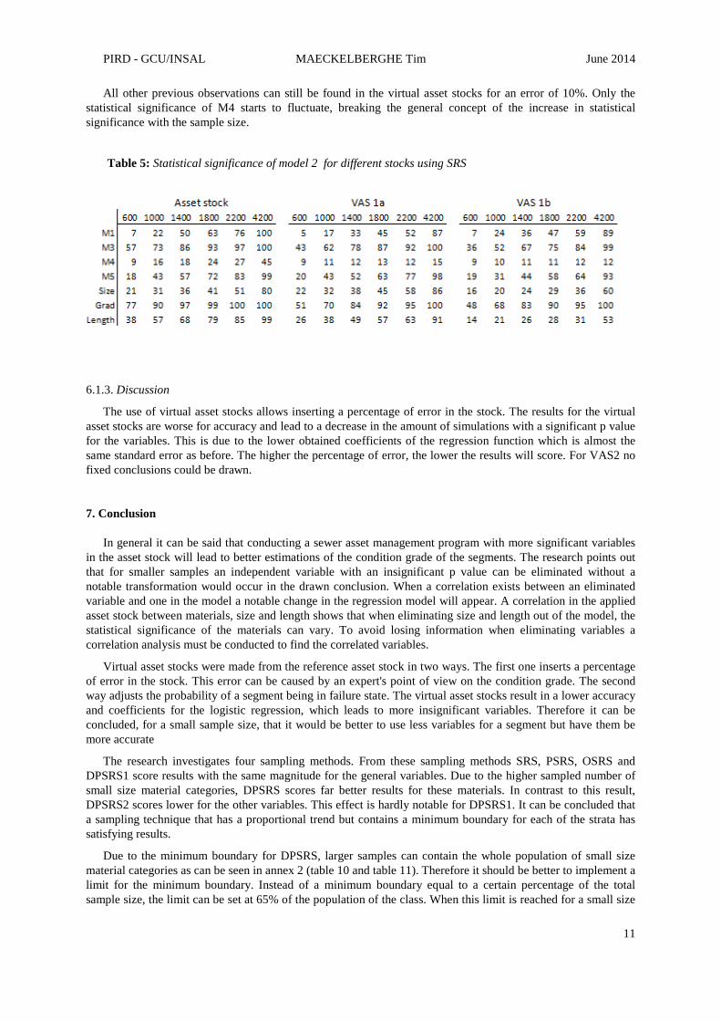
The introduced errors cause a decrease of the statistical significance in VAS1 for all sampling methods. The higher the error in the virtual asset stock, the bigger the decrease will be. Some variables are more exposed to the decrease than others. Table 5 shows that the variable size rests stable when introducing an error of 5%. By increasing the error to 10%, the variable size also will be affected. Even strong independent variables as gradient will diminish.

Despite the higher convergence the amount of simulations with a significant p value is generally still lower for the virtual asset stocks.

Changes were not notable for stronger, significant variables for VAS 2. Due to the different trend of the statistical significance for VAS 2a and VAS 2b, no fixed conclusions could be drawn for VAS 2. In VAS2a size shows a small decrease in the statistical significant (see annex 7, table 36), while for VAS2b M1, RCO and ST slightly decreased contrary to size which increased (see annex 7, table 37). When a modification occurs in the models, it could be found in all the sampling techniques.

Figure 6: Accuracy of model 0; variable=age - General stock (left), VAS1a (middle) and VAS1b (right)


11

All other previous observations can still be found in the virtual asset stocks for an error of 10%. Only the statistical significance of M4 starts to fluctuate, breaking the general concept of the increase in statistical significance with the sample size.

6.1.3. Discussion

The use of virtual asset stocks allows inserting a percentage of error in the stock. The results for the virtual asset stocks are worse for accuracy and lead to a decrease in the amount of simulations with a significant p value for the variables. This is due to the lower obtained coefficients of the regression function which is almost the same standard error as before. The higher the percentage of error, the lower the results will score. For VAS2 no fixed conclusions could be drawn.

7. Conclusion

In general it can be said that conducting a sewer asset management program with more significant variables in the asset stock will lead to better estimations of the condition grade of the segments. The research points out that for smaller samples an independent variable with an insignificant p value can be eliminated without a notable transformation would occur in the drawn conclusion. When a correlation exists between an eliminated variable and one in the model a notable change in the regression model will appear. A correlation in the applied asset stock between materials, size and length shows that when eliminating size and length out of the model, the statistical significance of the materials can vary. To avoid losing information when eliminating variables a correlation analysis must be conducted to find the correlated variables.

Virtual asset stocks were made from the reference asset stock in two ways. The first one inserts a percentage of error in the stock. This error can be caused by an expert's point of view on the condition grade. The second way adjusts the probability of a segment being in failure state. The virtual asset stocks result in a lower accuracy and coefficients for the logistic regression, which leads to more insignificant variables. Therefore it can be concluded, for a small sample size, that it would be better to use less variables for a segment but have them be more accurate

The research investigates four sampling methods. From these sampling methods SRS, PSRS, OSRS and DPSRS1 score results with the same magnitude for the general variables. Due to the higher sampled number of small size material categories, DPSRS scores far better results for these materials. In contrast to this result, DPSRS2 scores lower for the other variables. This effect is hardly notable for DPSRS1. It can be concluded that a sampling technique that has a proportional trend but contains a minimum boundary for each of the strata has satisfying results.

Due to the minimum boundary for DPSRS, larger samples can contain the whole population of small size material categories as can be seen in annex 2 (table 10 and table 11). Therefore it should be better to implement a limit for the minimum boundary. Instead of a minimum boundary equal to a certain percentage of the total sample size, the limit can be set at 65% of the population of the class. When this limit is reached for a small size

Table 5: Statistical significance of model 2 for different stocks using SRS


12

material category, new samples will be drawn from the bigger classes. It allows for a better estimation of the regression coefficients from the bigger classes, which are more decisive.

Better estimations for the true value will be obtained for larger samples sizes. The graphs from the results of the statistical analysis test show an exponential trend. The curves in the graphs for the research flatten out after n=2000. Which leads to the conclusion that satisfactory results can be obtained for a sample size of 2000. With this sample size, 1/5 of the asset stock is examined.

8. Outlook

Due to the inefficiency and costly inspection for the investigated sample methods, more practical sampling methods should be elaborated. Cluster sampling with districts as clusters is a practical suitable method, but will not obtain as precise results as PSRS (Lohr, 2010). Randomly inspecting several segments from some districts is more cost efficient than randomly selecting segments throughout the whole municipality. Districts are built in the same period and contain segments with similar characteristics (Ahmadi, 2014). The sample can be adjusted during the inspection so that every material class respects the minimum boundary. The absence of district information in the asset stock rejected the insertion of this method in the research.

Further research should be done with different asset stocks. Stocks with other variables can conclude a that certain variables are more important for predicting the condition grade. This general set can potentially be supplemented with significant variables related to the location of the asset stock. An example is Dirksen who introduced settlement data for segments located in soft soil as variables (Dirksen et al., 2014).

The asset stock is inspired on the metropolitan sewer district of the Greater Cincinnati as according to (Salman, 2010). However this asset stock contains no information about rehabilitated segments, which will be the result from sewer asset management strategies. A way to inspect and implement these segments in the stocks can be a goal for further research.

To optimistic hypotheses was taken for the generation of virtual asset stocks with method 2. It led to no fixed results due to the low degree of error implemented in the asset stock. Further research has to be conducted to better determine the relationship between the attributes and the condition grade.

I would like to thank the people who gave me the opportunity to study abroad and made this PIRD possible. In particularly I would like to thank Mr. Le Gauffre P. for the numerous hours he spent to indicate me in the work.


13

References Agresti, A. (2002). Categorical data analysis, 2nd Ed. Hoboken, NJ: Wiley.

Ahmadi, M. (2014). Sewer Asset Management: Impact of Data Quality and Models' Parameters on Condition Assessment of Assets and Asset Stocks. Thesis (PhD), L'institut national des sciences appliquées de Lyon, Lyon.

Ana, E., Bauwens, W., Pessemier, M., Thoeye, C., Smolders, S., Boonen, I., and De Geuldre, G. (2009). "An investigation of factors influencing sewer structural deterioration.", Urban Water Journal, 6(4), 303-312.

Ariaratnam, S., El-Assaly, A., and Yang, Y. (2001). “Assessment of infrastructure inspection needs using logistic models.” Journal of Infrastructure Systems., 7(4), 160 -165.

Baik, H.-S., Seok, H., and Abraham, D. M. (2006). “Estimating transition probabilities in markov chain-based deterioration models for management of wastewater systems.” Jounal of Water Resources Planning and Managemet., 132(1), 15 – 24.

Cochran, W. G. (1977). Sampling Techniques, 3th Ed. Cambridge , Massachusetts: Wiley.

Davies, J. P., Clarke, B. A., Whiter, J. T., Cunningham, R. J., and Leidi, A. (2001b). “The structural condition of rigid sewer pipes: a statistical investigation.” Urban Water Journal, 3(4), 277– 286.

Dirksen J., Egbert J. Baars, Jeroen G. Langeveld & Francois H.L.R. Clemens (2014) Quality and use of sewer invert measurements, Structure and Infrastructure Engineering: Maintenance, Management, Life-Cycle Design and Performance, 10:3, 295-304

Lohr S. L. (2010). Sampling: Design and Analysis, 2nd Ed. Boston, Massachusetts: Cengage Learning.

Peduzzi, P., Concato, J., Kemper, E., Holford, TR., Feinstein, A.R., (1996). “A simulation study of the number of events per variable in logistic regression analysis”. Journal of Clinical Epidemiologic; 49: 1373–1379.

Rakotomalala, R. (2011). Pratique de la Régression Logistique, 2nd Ed. Lyon, France: Université Lumière Lyon 2.

Salman, B., and Salem, O., (2012). “Modeling failure of wastewater collection lines using various section-level regression models”, Journal of Infrastructure Systems, ASCE, 18(2), 146-154.

Salman, B., (2010). “Infrastructure management and deterioration risk assessment of wastewater collection systems”. Thesis (PhD), University of Cincinnati, OH.

Syachrani, S., Jeong, H. S. D., and Chung, C. S. (2012). "Decision tree-based deterioration model for buried wastewater pipelines." Journal of Performance of Constructed Facilities, 27(12), 633-645.

Younis, R., and Knight, M. A. (2012). "Development and implementation of an asset management framework for wastewater collection networks.", Tunnelling and Underground Space Technology, 39 (2014), 130–143


14

Annexes

Summary

Annex 1: Remarks ............................................................................................................................................15

Annex 2: Material classes .................................................................................................................................16

Annex 3: Statistical significance for the first set of models .............................................................................18

Annex 4: Logistic regression coefficients ........................................................................................................20

Annex 5: Standard error ...................................................................................................................................22

Annex 6: Statistical significance for SRS & DPSRS1 .....................................................................................24

Annex 7: Virtual asset stocks............................................................................................................................26


15

Annex 1: Remarks

Remark 1

The precision and accuracy show differences for the model 1b, 2 and 3 comparing to the reference model and model 1 for the dependent variables. Model 1b, 2 and 3 show better results for precision and accuracy than the reference and model 1a. Even when the whole population of class M4 is present in the sample it can be seen that the precision for the reference and model 1a are not equal to 1.

When the whole stratum is sampled, the sample is expected to provide the true values for the stratum. According to formula 4, obtaining the true value will lead to a precision of 1, which is achieved by model 1b, 2 and 3 (see figure 7).

Remark 2

The results as seen in figure 8 from the convergence test indicate that for all the virtual asset stocks the amount of converged simulations increases with the degree of error. The convergence is larger with error than without error, see figure 1. This increase is notable for every sampling method, model and sample size. Due to the minority of segments in failure state, randomly adjusting the condition grade will lead to more segments in failure state. This results in more samples for the small size material categories with both the condition grades, which is the main requirement to form the logistic regression function.

Figure 7: Precision of methods for M4 n=4200

Figure 8: Amount of converged simulation per sample size; VAS1a left, VAS1b right


16

Annex 2: Material classes

Table 6: Correlation table for size and length

Table 7: Percentage of sample size for each material class for SRS

Table 8: Percentage of sample size for each material class for PSRS

Table 9: Percentage of sample size for each material class for OSRS


17

Table 10: Percentage of sample size for each material class for DPSRS1

Table 11: Percentage of sample size for each material class for DPSRS2


18

Annex 3: Statistical significance for the first set of models

Table 12: Model 1 - Statistical significance of the coefficients per converged simulations in percentage for different sample sizes calculated with SRS




19



20

Annex 4: Logistic regression coefficients

Table 16: Regression coefficients - set 1

B0 Age M1 M3 M4 M5 Size Depth Grad RCO Length ST

Ref. Model -3,353 0,0219 -1,223 -0,557 -0,449 -0,837 -0,00079 -0,042 0,0686 0,268 0,0131 0,246

Model 1 -3,591 0,0218 -1,492 -0,568 -0,804 0,0686 0,272 0,0083 0,232

Model 2 -3,382 0,0217 -1,480 -0,557 -0,801 0,0687 0,0084

Model 3 -3,400 0,0212 -0,508 0,0684 0,0088

Model 4 -3,234 0,0212 -0,380 0,0680

Table 17: Regression coefficients - set 2


Ref. Model -3,353 0,0219 -1,223 -0,557 -0,449 -0,837 -0,00079 -0,042 0,0686 0,268 0,0131 0,246

Model1a -3,251 0,0218 -1,236 -0,554 -0,469 -0,827 -0,00072 0,0686 0,0132

Model 1b -3,424 0,0218 -1,473 -0,460 -0,329 -0,866 0,0681 0,269 0,237

Model 2 -3,211 0,0217 -1,461 -0,447 -0,321 -0,863 0,0682

Model 3 -2,924 0,0217 -1,440 -0,441 -0,332 -0,864

Table 18: Regression coefficients - VAS 1a


Ref. Model -2,597 0,0169 -0,854 -0,459 -0,224 -0,713 -0,00077 -0,034 0,0483 0,216 0,0095 0,186

Model1a -2,526 0,0169 -0,865 -0,458 -0,242 -0,708 -0,00072 0,0484 0,0096

Model 1b -2,712 0,0169 -1,120 -0,419 -0,214 -0,727 0,0480 0,218 0,178

Model 2 -2,551 0,0168 -1,112 -0,410 -0,210 -0,727 0,0482

Model 3 -2,356 0,0168 -1,104 -0,407 -0,217 -0,730

Table 19: Regression coefficients - VAS 1b


Ref. Model -2,221 0,0143 -0,854 -0,380 -0,212 -0,585 -0,00054 -0,025 0,0458 0,177 0,0056 0,140

Model1a -2,166 0,0143 -0,863 -0,379 -0,226 -0,582 -0,00050 0,0459 0,0057

Model 1b -2,326 0,0143 -1,049 -0,371 -0,242 -0,590 0,0457 0,179 0,135

Model 2 -2,203 0,0142 -1,043 -0,364 -0,239 -0,590 0,0458

Model 3 -2,019 0,0143 -1,036 -0,362 -0,246 -0,595


21

Table 20: Regression coefficients - VAS 2a


Ref. Model -3,387 0,0220 -1,182 -0,569 -0,413 -0,773 -0,00070 -0,042 0,0702 0,289 0,0127 0,230

Model 1a -3,289 0,0219 -1,195 -0,566 -0,434 -0,764 -0,00064 0,0702 0,0129

Model 1b -3,441 0,0219 -1,402 -0,465 -0,274 -0,803 0,0697 0,291 0,223

Model 2 -3,232 0,0218 -1,390 -0,453 -0,267 -0,802 0,0698

Model 3 -2,938 0,0218 -1,369 -0,447 -0,279 -0,804

Table 21: Regression coefficients - VAS 2b


Ref. Model -3,273 0,0215 -0,978 -0,562 -0,451 -0,848 -0,00091 -0,041 0,0739 0,225 0,0127 0,216

Model 1a -3,197 0,0215 -0,991 -0,561 -0,469 -0,839 -0,00085 0,0739 0,0128

Model 1b -3,379 0,0214 -1,277 -0,487 -0,384 -0,871 0,0734 0,227 0,206

Model 2 -3,197 0,0214 -1,268 -0,476 -0,376 -0,869 0,0735

Model 3 -2,886 0,0213 -1,247 -0,469 -0,388 -0,87


22

Annex 5: Standard error

Table 22: SE

B0 Age M1 M3 M4 M5 Size Depth Gradient RC Length ST

Ref. Model 0,136 0,00097 0,282 0,0814 0,197 0,175 0,00021 0,021 0,00748 0,0608 0,00246 0,0534

Model 1a 0,121 0,00097 0,282 0,0812 0,196 0,174 0,00021 0,00745 0,00245

Model 1b 0,104 0,00097 0,269 0,0638 0,161 0,174 0,00746 0,0606 0,0531

Model 2 0,096 0,00096 0,268 0,0636 0,161 0,174 0,00743

Model 3 0,090 0,00096 0,267 0,0633 0,160 0,173

Table 23: SE of VAS 1a


Ref. Model 0,124 0,0009 0,243 0,0760 0,182 0,159 0,00020 0,0195 0,0072 0,0581 0,00231 0,0503

Model 1a 0,110 0,0009 0,243 0,0759 0,181 0,159 0,00020 0,0072 0,00230

Model 1b 0,094 0,0009 0,229 0,0602 0,149 0,158 0,0072 0,0580 0,0501

Model 2 0,086 0,0009 0,229 0,0600 0,149 0,158 0,0072

Model 3 0,081 0,0009 0,228 0,0599 0,149 0,158

Table 24: SE of VAS 1b


Ref. Model 0,118 0,0008 0,231 0,0725 0,175 0,1470 0,00019 0,0188 0,0070 0,0564 0,0022 0,0484

Model 1a 0,104 0,0008 0,231 0,0724 0,175 0,1468 0,00019 0,0070 0,0022

Model 1b 0,088 0,0008 0,218 0,0576 0,146 0,1464 0,0070 0,0563 0,0483

Model 2 0,081 0,0008 0,218 0,0575 0,145 0,1462 0,0070

Model 3 0,076 0,0008 0,217 0,0574 0,145 0,1459

Table 25: SE of VAS 2a


Ref. Model 0,136 0,00097 0,276 0,082 0,195 0,172 0,0002 0,0207 0,00747 0,0607 0,00246 0,0533

Model 1a 0,121 0,00097 0,275 0,081 0,195 0,171 0,0002 0,00745 0,00245

Model 1b 0,104 0,00097 0,262 0,064 0,159 0,171 0,00746 0,0605 0,0531

Model 2 0,097 0,00097 0,261 0,064 0,159 0,171 0,00743

Model 3 0,090 0,00096 0,260 0,063 0,158 0,170


23

Table 26: SE of VAS 2b


Ref. Model 0,135 0,00097 0,265 0,0815 0,198 0,175 0,00021 0,0206 0,0075 0,0610 0,00246 0,053

Model 1a 0,121 0,00096 0,264 0,0813 0,198 0,174 0,00021 0,0074 0,00246

Model 1b 0,104 0,00096 0,250 0,0641 0,163 0,174 0,0074 0,0608 0,053

Model 2 0,096 0,00096 0,249 0,0639 0,163 0,174 0,0074

Model 3 0,089 0,00096 0,248 0,0636 0,162 0,173


24

Annex 6: Statistical significance for SRS & DPSRS1

Table 27: SRS - Reference Model : Percentage of converged simulations with a significant p value which is also displayed in the work of (Ahmadi, 2014)

Table 28: SRS - Model 1a: Percentage of converged simulations with a significant p value

Table 29: SRS - Model 1b: Percentage of converged simulations with a significant p value

Table 30: SRS - Model 2: Percentage of converged simulations with a significant p value


25

Table 31: DPSRS1 - Reference Model: Percentage of converged simulations with a significant p value

Table 32: DPSRS1 - Model 1a: Percentage of converged simulations with a significant p value

Table 33: DPSRS1 - Model 1b: Percentage of converged simulations with a significant p value


26

Annex 7: Virtual asset stocks

Table 34: Number of adjusted segments from reference stock to VAS 2

Class (units) Total (9810) M1 (160) M2 (6824) M3 (2245) M4 (265) M5 (316)

VAS2a 75 5 41 21 4 4

VAS2b 174 5 110 35 12 12

Table 35: Statistical significance of VAS 1 for SRS

Reference Model - VAS 1a

Reference Model - VAS 1b

Var / n 600 1000 1400 1800 2200 4200

600 1000 1400 1800 2200 4200

Intercept 100 100 100 100 100 100

100 100 100 100 100 100

Age 100 100 100 100 100 100

100 100 100 100 100 100

M1 17 32 43 52 62 86

8 24 37 48 57 90

M3 61 76 85 91 96 100

38 51 62 73 84 99

M4 10 12 13 11 12 13

8 8 10 11 10 13

M5 41 54 65 74 82 98

18 33 44 53 63 92

Size 33 42 53 59 67 88

17 20 28 29 36 60

Depth 13 15 14 19 20 25

8 11 11 14 12 16

Gradient 70 82 91 95 97 100

50 67 80 88 94 100

RCO 33 42 48 53 62 83

22 27 32 35 41 71

Length 32 44 55 66 69 91

18 20 21 22 28 49

ST 32 39 45 55 60 84

16 23 28 32 36 61

Table 36: Comparison of the statistical significance of the reference to VAS 2a for SRS

Reference Model

Reference Model - VAS 2a

Var / n 600 1000 1400 1800 2200 4200

600 1000 1400 1800 2200 4200

Intercept 100 100 100 100 100 100

100 100 100 100 100 100

Age 100 100 100 100 100 100

100 100 100 100 100 100

M1 8 26 47 62 75 99

7 24 43 63 72 99

M3 53 75 88 93 98 100

55 76 87 95 98 100

M4 9 16 18 21 23 42

9 15 16 21 22 38

M5 22 43 60 73 84 100

15 39 55 65 78 98

Size 27 32 38 50 58 87

23 26 36 43 50 77

Depth 15 19 15 18 22 35

12 13 19 17 23 36

Gradient 73 90 98 100 100 100

76 92 98 100 100 100

RCO 27 39 51 62 67 94

27 46 58 68 74 97

Length 38 53 68 76 84 99

36 49 63 77 82 99

ST 30 41 55 62 75 97

28 39 48 60 69 94


27

Table 37: Comparison of the statistical significance of the reference to VAS 2b for SRS

Reference Model

Reference Model - VAS 2b

Var / n 600 1000 1400 1800 2200 4200

600 1000 1400 1800 2200 4200

Intercept 100 100 100 100 100 100

100 100 100 100 100 100

Age 100 100 100 100 100 100

100 100 100 100 100 100

M1 8 26 47 62 75 99

4 18 34 48 57 91

M3 53 75 88 93 98 100

52 75 87 94 98 100

M4 9 16 18 21 23 42

9 16 20 22 24 44

M5 22 43 60 73 84 100

21 47 62 72 85 99

Size 27 32 38 50 58 87

27 40 48 57 69 94

Depth 15 19 15 18 22 35

12 18 18 17 21 34

Gradient 73 90 98 100 100 100

80 92 99 100 100 100

RCO 27 39 51 62 67 94

19 32 41 49 55 84

Length 38 53 68 76 84 99

35 51 62 75 80 99

ST 30 41 55 62 75 97

28 34 45 53 65 91

Sewer asset management: impact of sample size and ...

Documents

Transcript of Sewer asset management: impact of sample size and ...