+ Chapter 6: Random Variables Section 6.2 Transforming and Combining Random Variables.

Several Random Variables
Dr. Edmund Lam
Department of Electrical and Electronic Engineering
The University of Hong Kong
ELEC2844: Probabilistic Systems Analysis
(Second Semester, 2020{21)
https://www.eee.hku.hk/~elec2844
E. Lam (University of Hong Kong) ELEC2844 Jan{Apr, 2021 1 / 98

Multiple random variables
We have mostly looked at one random variable X, including whether it
is discrete or continuous.
We have also looked at multiple random variables brie y, discussing:
Joint PMF / PDF and marginal PMF / PDF
Conditional PMF / PDF and independence
Expectation and variance of the sum of independent random
variables
Bayes' rule
In this lecture, we will further investigate topics relating to multiple
random variables.
E. Lam (University of Hong Kong) ELEC2844 Jan{Apr, 2021 2 / 98

Derived distributions
1 Derived distributions
2 Sum of random variables
3 Covariance and correlation
Covariance
A detailed example
Correlation
4 Gaussian random variables
Central limit theorem
Higher dimensional Gaussian
Generalization of Gaussian random variable
5 (Advanced Topic) Expectation and variance
Iterated expectation
Total variance
6 (Advanced Topic) Random number of independent random variables
E. Lam (University of Hong Kong) ELEC2844 Jan{Apr, 2021 3 / 98

Derived distributions
Procedure
The procedure for transforming one random variable to another is
applicable to several random variables.
Given: PDF of X and Y, and Z = g(X, Y), �nd the PDF of Z.
A two-step procedure:
FZ(z) = P(Z 6 z) = P(g(X, Y) 6 z) =∫∫
{x,y |g(x,y)6z}
fX,Y(x, y)dxdy
fZ(z) =d
dzFZ(z)
(1)
(2)
E. Lam (University of Hong Kong) ELEC2844 Jan{Apr, 2021 4 / 98

Derived distributions
Example
X ∼ U(0, 1) and Y ∼ U(0, 1), X and Y are independent, and
Z = max{X, Y}. What is the PDF of Z?
ANS: We know P(X 6 z) = P(Y 6 z) = z.
FZ(z) = P(max{X, Y} 6 z) = P(X 6 z, Y 6 z)
= P(X 6 z)P(Y 6 z) = z2
Di�erentiating,
fZ(z) =
{2z 0 6 z 6 1
0 otherwise.
E. Lam (University of Hong Kong) ELEC2844 Jan{Apr, 2021 5 / 98

Derived distributions
Example
X ∼ U(0, 1) and Y ∼ U(0, 1), X and Y are independent, and Z = Y/X.
What is the PDF of Z?
ANS: Case 1: 0 6 z 6 1. We need to �nd P(YX 6 z
)= P(Y 6 zX).
Given X = x, we have P(Y 6 zX) = zx. But we need to integrate over
all possible values of X. Therefore,
P(Y 6 zX) =∫10(zx)dx =
[12zx
2]10= 12z.
Case 2: z > 1. Let z ′ = 1/z.
P(Y/X 6 z) = P(X/Y > z ′
)= 1− P
(X/Y 6 z ′
)= 1− 1
2z′ = 1− 1
2z
y
x0
1
1
z
y
x0
1
1
1z
E. Lam (University of Hong Kong) ELEC2844 Jan{Apr, 2021 6 / 98

Derived distributions
Example
Combining,
FZ(z) = P(Y
X6 z
)=
z2 0 6 z 6 1
1− 12z z > 1
0 otherwise.
Di�erentiating,
fZ(z) =
12 0 6 z 6 112z2
z > 1
0 otherwise.
E. Lam (University of Hong Kong) ELEC2844 Jan{Apr, 2021 7 / 98

Derived distributions
Example
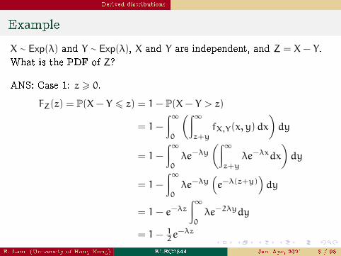
X ∼ Exp(λ) and Y ∼ Exp(λ), X and Y are independent, and Z = X− Y.
What is the PDF of Z?
ANS: Case 1: z > 0.
FZ(z) = P(X− Y 6 z) = 1− P(X− Y > z)
= 1−
∫∞0
(∫∞z+y
fX,Y(x, y)dx
)dy
= 1−
∫∞0
λe−λy(∫∞z+y
λe−λxdx
)dy
= 1−
∫∞0
λe−λy(e−λ(z+y)
)dy
= 1− e−λz∫∞0
λe−2λydy
= 1− 12e
−λz
E. Lam (University of Hong Kong) ELEC2844 Jan{Apr, 2021 8 / 98
Derived distributions
Example
X ∼ Exp(λ) and Y ∼ Exp(λ), X and Y are independent, and Z = X− Y.
What is the PDF of Z?
ANS: Case 1: z > 0.
FZ(z) = P(X− Y 6 z) = 1− P(X− Y > z)
= 1−
∫∞0
(∫∞z+y
fX,Y(x, y)dx
)dy
= 1−
∫∞0
λe−λy(∫∞z+y
λe−λxdx
)dy
= 1−
∫∞0
λe−λy(e−λ(z+y)
)dy
= 1− e−λz∫∞0
λe−2λydy
= 1− 12e
−λz
E. Lam (University of Hong Kong) ELEC2844 Jan{Apr, 2021 8 / 98

Derived distributions
Example
Case 2: z < 0. Then, −Z = Y −X which has the same distribution as Z.
FZ(z) = P(Z 6 z) = P(−Z > −z) = P(Z > −z) = 1− FZ(−z)
Since −z > 0, we can make use of case 1,
FZ(z) = 1−(1− 1
2e−λ(−z)
)= 12eλz
y
x
x− y = z
z > 0
y
x
x− y = z
z < 0
E. Lam (University of Hong Kong) ELEC2844 Jan{Apr, 2021 9 / 98

Derived distributions
Example
Combining,
FZ(z) =
{1− 1
2e−λz z > 0
12eλz z < 0
Di�erentiating,
fZ(z) =
{λ2e
−λz z > 0λ2eλz z < 0
We can express in a single formula
fZ(z) =λ
2e−λ|z| (3)
called Laplacian random variable, and denote Z ∼ Lap(λ).
E. Lam (University of Hong Kong) ELEC2844 Jan{Apr, 2021 10 / 98

Derived distributions
(4) Laplacian random variable
We can add Laplacian to our list of continuous random variables.
mean: E(X) variance: var(X)
Laplacian: X ∼ Lap(λ) 02
λ2
fX(x)
x
E. Lam (University of Hong Kong) ELEC2844 Jan{Apr, 2021 11 / 98

Derived distributions
(4) Laplacian random variable
E(X) = 0 (by symmetry)
var(X) = 2
(∫∞0
x2λ
2e−λxdx
)= λ
[(−x2
λ−2x
λ2−2
λ3
)e−λx
]∞0
=2
λ2
MX(s) =
∫∞−∞ esx
λ
2e−λ|x|dx
=λ
2
[∫0−∞ esxeλxdx+
∫∞0
esxe−λxdx
]
=λ
2
{[1
s+ λe(s+λ)x
]0−∞ +
[1
s− λe(s−λ)x
]∞0
}
=λ
2
(1
s+ λ−
1
s− λ
)=
λ2
λ2 − s2where |s| < λ
E. Lam (University of Hong Kong) ELEC2844 Jan{Apr, 2021 12 / 98

Derived distributions
Example
X ∼ N(0, 1) and Y ∼ N(0, 1), X and Y are independent, and Z = X+ iY,
where i =√−1. What are the PDFs of |Z| and ∠Z?
ANS: We work out the solution in a few steps.
Step 1: Representing X and Y in a complex plane, we can convert to
polar coordinates with random variables R > 0 and Θ ∈ [0, 2π], where
X = R cosΘ Y = R sinΘ
We also note that the joint PDF of X and Y is
fX,Y(x, y) = fX(x) fY(y) =1
2πe−(x2+y2)/2
E. Lam (University of Hong Kong) ELEC2844 Jan{Apr, 2021 13 / 98

Derived distributions
Example
Step 2: From fX,Y(x, y) we �nd FR,Θ(r, θ).
For a �xed set of (r, θ), the CDF integrates all the points (s, φ) with
0 6 s 6 r and 0 6 φ 6 θ, which is a sector of a circle with radius r
and angle θ, denoted A.
FR,Θ(r, θ) = P(R 6 r, Θ 6 θ)
=
∫∫A
1
2πe−(x2+y2)/2dxdy
=1
2π
∫θ0
∫r0
e−s2/2sdsdφ
E. Lam (University of Hong Kong) ELEC2844 Jan{Apr, 2021 14 / 98

Derived distributions
Example
Step 3: Di�erentiate FR,Θ(r, θ) to obtain fR,Θ(r, θ).
fR,Θ(r, θ) =∂2
∂r∂θFR,Θ(r, θ) =
r
2πe−r
2/2 r > 0, θ ∈ [0, 2π]
Step 4: Integrate joint PDF to �nd marginal PDF
fR(r) =
∫2π0
fR,Θ(r, θ)dθ = re−r2/2 r > 0
fΘ(θ) =
∫∞0
r
2πe−r
2/2dr =1
2π
[− e−r
2/2]∞0
=1
2πθ ∈ [0, 2π]
In our question, |Z| = R and ∠Z = Θ
E. Lam (University of Hong Kong) ELEC2844 Jan{Apr, 2021 15 / 98

Derived distributions
Example
X ∼ N(0, 1) and Y ∼ N(0, 1), X and Y are independent, and Z = X+ iY,
then
1 The angle follows a uniform distribution, Θ ∼ U(0, 2π)
2 The magnitude follows a distribution known as Rayleigh
distribution, R ∼ Ray(σ) where
fR(r) =r
σ2e−r
2/(2σ2) (4)
with σ2 being the variance of the normal distributions X and Y.
E. Lam (University of Hong Kong) ELEC2844 Jan{Apr, 2021 16 / 98

Derived distributions
(5) Rayleigh random variable
We can add Rayleigh to our list of continuous random variables.
mean: E(X) variance: var(X)
Rayleigh: X ∼ Ray(σ) σ
√π
2
4− π
2σ2
fX(x)
x
E. Lam (University of Hong Kong) ELEC2844 Jan{Apr, 2021 17 / 98

Sum of random variables
1 Derived distributions
2 Sum of random variables
3 Covariance and correlation
Covariance
A detailed example
Correlation
4 Gaussian random variables
Central limit theorem
Higher dimensional Gaussian
Generalization of Gaussian random variable
5 (Advanced Topic) Expectation and variance
Iterated expectation
Total variance
6 (Advanced Topic) Random number of independent random variables
E. Lam (University of Hong Kong) ELEC2844 Jan{Apr, 2021 18 / 98

Sum of random variables
Sum of two independent random variables
X and Y are two random variables, possibly of di�erent distributions,
but independent of each other. We are interested to know the
distribution of Z = X+ Y.
Discrete random variables:
pZ(z) = P(X+ Y = z) =∑
{(x,y) |x+y=z}
P(X = x, Y = y)
=∑x
P(X = x, Y = z− x)
=∑x
P(X = x)P(Y = z− x)
=∑x
pX(x)pY(z− x)
E. Lam (University of Hong Kong) ELEC2844 Jan{Apr, 2021 19 / 98

Sum of random variables
Sum of two independent random variables
Continuous random variables:
P(Z 6 z |X = x) = P(X+ Y 6 z |X = x)
= P(x+ Y 6 z |X = x)
= P(x+ Y 6 z)
= P(Y 6 z− x)
Di�erentiating, we get fZ |X(z | x) = fY(z− x).
fX,Z(x, z) = fX(x) fZ |X(z | x) = fX(x) fY(z− x)
fZ(z) =
∫∞−∞ fX,Z(x, z)dx =
∫∞−∞ fX(x) fY(z− x)dx
E. Lam (University of Hong Kong) ELEC2844 Jan{Apr, 2021 20 / 98
Sum of random variables
Sum of two independent random variables
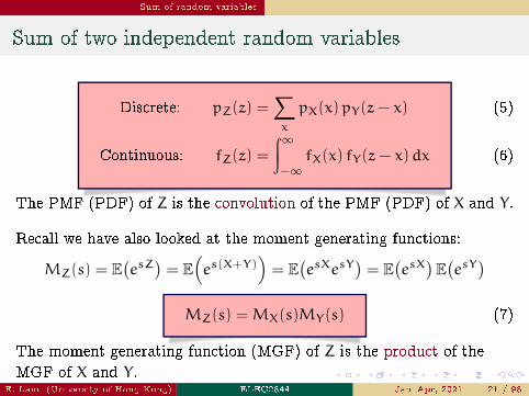
Discrete: pZ(z) =∑x
pX(x)pY(z− x)
Continuous: fZ(z) =
∫∞−∞ fX(x) fY(z− x)dx
(5)
(6)
The PMF (PDF) of Z is the convolution of the PMF (PDF) of X and Y.
Recall we have also looked at the moment generating functions:
MZ(s) = E(esZ)= E
(es(X+Y)
)= E
(esXesY
)= E
(esX)E(esY)
MZ(s) =MX(s)MY(s) (7)
The moment generating function (MGF) of Z is the product of the
MGF of X and Y.E. Lam (University of Hong Kong) ELEC2844 Jan{Apr, 2021 21 / 98

Sum of random variables
Example
Two random variables X and Y are independent and uniformly
distributed between 0 and 1. Find the PDF of Z = X+ Y.
We make use of the formula
fZ(z) =
∫∞−∞ fX(x) fY(z− x)dx
=
∫10
fY(z− x)dx
since we know that only for 0 6 x 6 1, we have fX(x) = 1.
We also require 0 6 z− x 6 1 for fY(z− x) = 1. To see the resulting
limits of the integration, we divide into two cases: 0 6 z 6 1 and1 6 z 6 2.
E. Lam (University of Hong Kong) ELEC2844 Jan{Apr, 2021 22 / 98

Sum of random variables
Example
For 0 6 z 6 1, we need to enforce 0 6 z− x, which means the upper
limit of x can only be z:
fZ(z) =
∫10
fY(z− x)dx =
∫z0
(1)dx = z
For 1 6 z 6 2, we need to enforce z− x 6 1, which means the lower
limit of x can only be z− 1:
fZ(z) =
∫10
fY(z− x)dx =
∫1z−1
(1)dx = 1− (z− 1) = 2− z
We could have done the convolution graphically:
fZ(z)
z
fY(z− x)
z
fX(x)
fZ(z)
z1 2
1
0
E. Lam (University of Hong Kong) ELEC2844 Jan{Apr, 2021 23 / 98

Sum of random variables
Example
X ∼ Exp(λ) and Y ∼ Exp(λ), X and Y are independent, and Z = X− Y.
What is the PDF of Z?
ANS: We have already seen the answer is Laplacian. But we can also
proceed by noting that Z = X+ (−Y), and f−Y(y) = fY(−y) by
symmetry, so
fZ(z) =
∫∞−∞ fX(x) f−Y(z− x)dx =
∫∞−∞ fX(x) fY(x− z)dx
Now consider z > 0, so fY(x− z) is nonzero only when x > z.
fZ(z) =
∫∞z
λe−λxλe−λ(x−z)dx = λ2eλz∫∞z
e−2λxdx
= λ2eλz1
2λe−2λz =
λ
2e−λz
The case for z < 0 is similar.
E. Lam (University of Hong Kong) ELEC2844 Jan{Apr, 2021 24 / 98

Sum of random variables
Example
X ∼ Exp(λ) and Y ∼ Exp(λ), X and Y are independent, and Z = X− Y.
What is the PDF of Z?
ANS: We have already seen the answer is Laplacian. But we can also
proceed by noting that Z = X+ (−Y), and f−Y(y) = fY(−y) by
symmetry, so
fZ(z) =
∫∞−∞ fX(x) f−Y(z− x)dx =
∫∞−∞ fX(x) fY(x− z)dx
Now consider z > 0, so fY(x− z) is nonzero only when x > z.
fZ(z) =
∫∞z
λe−λxλe−λ(x−z)dx = λ2eλz∫∞z
e−2λxdx
= λ2eλz1
2λe−2λz =
λ
2e−λz
The case for z < 0 is similar.E. Lam (University of Hong Kong) ELEC2844 Jan{Apr, 2021 24 / 98
Covariance and correlation Covariance
1 Derived distributions
2 Sum of random variables
3 Covariance and correlation
Covariance
A detailed example
Correlation
4 Gaussian random variables
Central limit theorem
Higher dimensional Gaussian
Generalization of Gaussian random variable
5 (Advanced Topic) Expectation and variance
Iterated expectation
Total variance
6 (Advanced Topic) Random number of independent random variables
E. Lam (University of Hong Kong) ELEC2844 Jan{Apr, 2021 25 / 98

Covariance and correlation Covariance
De�nition
The covariance of two random variables X and Y is denoted by
cov(X, Y), and is de�ned by
cov(X, Y) = E[(X− E[X]
)(Y − E[Y]
)](8)
cov(X, Y) = 0 =⇒ X and Y are uncorrelated.
cov(X, Y) is positive =⇒ X− E(X) and Y − E(Y) tend to have the
same sign.
cov(X, Y) is negative =⇒ X− E(X) and Y − E(Y) tend to have the
opposite sign.
Variance measures the \spread" of a random variable. Covariance
measures the \spread" across two random variables.
E. Lam (University of Hong Kong) ELEC2844 Jan{Apr, 2021 26 / 98

Covariance and correlation Covariance
De�nition
Alternative form:
cov(X, Y) = E[XY] − E[X]E[Y] (9)
Proof:
cov(X, Y) = E[(X− E[X]
)(Y − E[Y]
)]= E(XY − XE[Y] − YE[X] + E[X]E[Y])= E[XY] − E[X]E[Y] − E[X]E[Y] + E[X]E[Y]= E[XY] − E[X]E[Y]
E. Lam (University of Hong Kong) ELEC2844 Jan{Apr, 2021 27 / 98

Covariance and correlation Covariance
Properties
Some properties (a and b are scalars):
cov(X,X) = var(X)
cov(X, aY + b) = a · cov(X, Y)cov(X, Y + Z) = cov(X, Y) + cov(X,Z)
(10)
(11)
(12)
Also, since if X and Y are independent, E[XY] = E[X]E[Y], so
X and Y independent =⇒ X and Y uncorrelated
Converse is NOT true! (illustrated in the next example)
E. Lam (University of Hong Kong) ELEC2844 Jan{Apr, 2021 28 / 98

Covariance and correlation Covariance
Example
Consider four points, at (1, 0), (0, 1), (−1, 0), (0,−1), each with
probability 1/4.
They are not independent because �xing Y (e.g. Y = 1), it determines
X (X = 0).
However,
E(X) = E(Y) = 0E(XY) = 0Hence, cov(X, Y) = 0
E. Lam (University of Hong Kong) ELEC2844 Jan{Apr, 2021 29 / 98

Covariance and correlation Covariance
Covariance
If X and Y are independent (uncorrelated),
var(X+ Y) = var(X) + var(Y). But more generally,
var(X+ Y) = var(X) + var(Y) + 2cov(X, Y) (13)
Even more generally,
var
(n∑i=1
Xi
)=
n∑i=1
var(Xi) +∑
{(i,j) | i 6=j}
cov(Xi, Xj
)(14)
E. Lam (University of Hong Kong) ELEC2844 Jan{Apr, 2021 30 / 98

Covariance and correlation Covariance
Covariance
Proof: Let Xi = Xi − E(Xi).
var
(n∑i=1
Xi
)= var
(n∑i=1
Xi
)= E
( n∑i=1
Xi
)2= E
n∑i=1
n∑j=1
XiXj
=
n∑i=1
n∑j=1
E[XiXj
]=
n∑i=1
E[X2i
]+
∑{(i,j) | i 6=j}
E[XiXj
]
=
n∑i=1
var(Xi) +∑
{(i,j) | i 6=j}
cov(Xi, Xj
)E. Lam (University of Hong Kong) ELEC2844 Jan{Apr, 2021 31 / 98

Covariance and correlation A detailed example
1 Derived distributions
2 Sum of random variables
3 Covariance and correlation
Covariance
A detailed example
Correlation
4 Gaussian random variables
Central limit theorem
Higher dimensional Gaussian
Generalization of Gaussian random variable
5 (Advanced Topic) Expectation and variance
Iterated expectation
Total variance
6 (Advanced Topic) Random number of independent random variables
E. Lam (University of Hong Kong) ELEC2844 Jan{Apr, 2021 32 / 98

Covariance and correlation A detailed example
Example
In a class with n students, after the �nal exam, they were ranked from
1 to n (no two students shared the same rank). The names and the
marks were put in a spreadsheet, but a careless teacher sorted the
names in some random way without linking them to the marks.
Consequently, the matching between the student and his or her actual
rank became random. For the student originally with rank k, the new
rank now takes a discrete random variable which is uniform between 1
and n. Note that in the new rank, again no two students share the
same rank.
What is the expected number of correct ranking (i.e., new rank is the
same as original rank), and its variance?
This question is a work of �ction. Any resemblance to actual
persons, living or dead, or actual events is purely coincidental.
E. Lam (University of Hong Kong) ELEC2844 Jan{Apr, 2021 33 / 98

Covariance and correlation A detailed example
Example
Attempt #1: Test some small cases. Let X = correct ranking.
1 Two students AB; after the randomization, half the time the order
remains AB; half the time the order becomes BA.
E(X) = 12 · (2) +
12 · (0) = 1
E(X2)= 12 · (2)
2 + 12 · (0)
2 = 2
var(X) = 2− 12 = 1
2 Three students ABC; There are now 3! permutations, with 1/6
being all correct, 3/6 having one correct, and 2/6 being all wrong.
E(X) = 16 · (3) +
36 · (1) +
26 · (0) = 1
E(X2)= 16 · (3)
2 + 36 · (1)
2 + 26 · (0)
2 = 2
var(X) = 2− 12 = 1
Guess: E(X) = var(X) = 1 for all n?E. Lam (University of Hong Kong) ELEC2844 Jan{Apr, 2021 34 / 98

Covariance and correlation A detailed example
Example
Attempt #2: Analytical derivation.
Let Xi = 1 if the ith student has the correct rank, and zero otherwise.
So,
X = X1 + X2 + . . .+ Xn
For each Xi, we have P(Xi = 1) = 1/n; therefore,
E(Xi) = 1n · 1+
n−1n · 0 = 1
n
E(X) = E(X1) + . . .+ E(Xn) = 1n + . . .+ 1
n = 1
Hence, although each one having a correct rank decreases with n, there
are more students, and the net result is that the expected number of
correctness remains 1.
E. Lam (University of Hong Kong) ELEC2844 Jan{Apr, 2021 35 / 98

Covariance and correlation A detailed example
Example
The calculation of the variance is more complicated because Xi and Xjare correlated, for i 6= j. First,
var(Xi) =1
n
(1−
1
n
)(Bernoulli)
Then, let us calculate E(XiXj
)for i 6= j.
E(XiXj
)= P
(Xi = 1 and Xj = 1
)= P(Xi = 1)P
(Xj = 1 |Xi = 1
)=1
n· 1
n− 1=
1
n(n− 1)
Hence,
cov(Xi, Xj
)= E
(XiXj
)− E(Xi)E
(Xj)=
1
n(n− 1)−1
n· 1n
=1
n2(n− 1)
E. Lam (University of Hong Kong) ELEC2844 Jan{Apr, 2021 36 / 98

Covariance and correlation A detailed example
Example
Overall,
var(X) = var
(n∑i=1
Xi
)=
n∑i=1
var(Xi) +∑
{(i,j) | i 6=j}
cov(Xi, Xj
)= n
[1
n
(1−
1
n
)]+ n(n− 1)
[1
n2(n− 1)
]= 1
Hence, the variance also remains 1 irrespective of the number of
students.
Quite surprising that irrespective of n, you always expect to get 1
correct and all the rest wrong, and even with the same variance!
E. Lam (University of Hong Kong) ELEC2844 Jan{Apr, 2021 37 / 98

Covariance and correlation Correlation
1 Derived distributions
2 Sum of random variables
3 Covariance and correlation
Covariance
A detailed example
Correlation
4 Gaussian random variables
Central limit theorem
Higher dimensional Gaussian
Generalization of Gaussian random variable
5 (Advanced Topic) Expectation and variance
Iterated expectation
Total variance
6 (Advanced Topic) Random number of independent random variables
E. Lam (University of Hong Kong) ELEC2844 Jan{Apr, 2021 38 / 98

Covariance and correlation Correlation
De�nition
Often, we work with a \normalized" version of covariance, known as
correlation coe�cient:
ρ(X, Y) =cov(X, Y)√var(X) var(Y)
(15)
Assuming X and Y both have nonzero variance, the numerator
determines similar properties as covariance:
ρ(X, Y) = 0 =⇒ X and Y are uncorrelated.
ρ(X, Y) is positive =⇒ X− E(X) and Y − E(Y) tend to have the
same sign.
ρ(X, Y) is negative =⇒ X− E(X) and Y − E(Y) tend to have the
opposite sign.
E. Lam (University of Hong Kong) ELEC2844 Jan{Apr, 2021 39 / 98

Covariance and correlation Correlation
De�nition
ρ(X, Y) is normalized in the sense that
−1 6 ρ(X, Y) 6 1 (16)
|ρ| is a measure of the extent to which X− E(X) and Y − E(Y) are\correlated" (i.e., cluster together).
|ρ| = 1 if and only if
Y − E[Y] = c(X− E[X]
)where c is a constant of the same sign as ρ
E. Lam (University of Hong Kong) ELEC2844 Jan{Apr, 2021 40 / 98

Covariance and correlation Correlation
Proof of correlation coe�cient magnitude (1)
We start with a lemma known as Schwarz inequality:
(E[XY]
)26 E
[X2]E[Y2]
(17)
for any random variable X and Y.
Proof: We assume E[Y2]6= 0, because otherwise we have Y = 0 with
probability 1, and therefore E[XY] = 0, so equality holds. With this
assumption, we start with an expression
E
[(X−
E[XY]E[Y2]
Y
)2]
which must be > 0.
E. Lam (University of Hong Kong) ELEC2844 Jan{Apr, 2021 41 / 98

Covariance and correlation Correlation
Proof of correlation coe�cient magnitude (2)
Proof:
0 6 E
[(X−
E[XY]E[Y2]
Y
)2]
= E[X2 − 2
E[XY]E[Y2]
XY +(E[XY])2
(E[Y2])2Y2]
= E[X2]− 2
E[XY]E[Y2]
E[XY] +(E[XY])2
(E[Y2])2E[Y2]
= E[X2]−
(E[XY])2
E[Y2]
Therefore,(E[XY]
)26 E
[X2]E[Y2], and thus
(E[XY]
)2E[X2]E[Y2]
6 1.
E. Lam (University of Hong Kong) ELEC2844 Jan{Apr, 2021 42 / 98

Covariance and correlation Correlation
Proof of correlation coe�cient magnitude (3)
For general random variables X and Y, we �rst \center" them to form
X = X− E[X]Y = Y − E[Y]
var(X)= var(X) = E
[X2]
cov(X, Y) = E[(X− E[X]
)(Y − E[Y]
)]= E
[XY]
Then, we make use of Schwarz inequality
(ρ(X, Y)
)2=
(cov(X, Y)
)2var(X) var(Y)
=
(E[XY] )2
E[X2]E[Y2] 6 1
So |ρ(X, Y)| 6 1.
E. Lam (University of Hong Kong) ELEC2844 Jan{Apr, 2021 43 / 98

Covariance and correlation Correlation
Proof of correlation coe�cient magnitude (4)
Next, we show what happens when Y −E[Y] = c(X−E[X]
), or Y = cX:
E(XY)= cE
(X2)
E(Y2)= c2E
(X2)
Therefore,
ρ(X, Y) =cE[X2]
√c2E
[X2]E[X2] =
c
|c|=
{1 c > 0
−1 c < 0
E. Lam (University of Hong Kong) ELEC2844 Jan{Apr, 2021 44 / 98

Covariance and correlation Correlation
Proof of correlation coe�cient magnitude (5)
We now show the reverse: when ρ(X, Y) = ±1,
E
X−
E[XY]
E[Y2] Y2 = E
[X2]−
(E[XY])2
E[Y2]
= E[X2] (1− [ρ(X, Y)]2
)= 0
This means, with probability 1, X−E[XY]E[Y2]
Y is equal to zero. It follows
that, with probability 1,
X =E[XY]
E[Y2] Y =
√√√√√E[X2]
E[Y2]ρ(X, Y)Y
i.e., the ratio of X and Y is determined by the sign of ρ(X, Y).E. Lam (University of Hong Kong) ELEC2844 Jan{Apr, 2021 45 / 98

Covariance and correlation Correlation
Example
For n independent coin toss, let X be the number of heads and Y be
the number of tails. What is the correlation coe�cient ρ(X, Y)?
ANS: Since X+ Y = n, they are \perfectly correlated." We expect
ρ(X, Y) = ±1. Moreover, since X+ Y = E(X) + E(Y) = n, we have
X− E(X) = −(Y − E(Y)
)so the sign of ρ(X, Y) should be negative, i.e., it is equal to −1.
Alternatively, we can apply the formula
cov(X, Y) = E[(X− E[X])(Y − E[Y])] = −E[(X− E[X])2
]= −var(X)
and note that var(X) = var(Y), by symmetry, and therefore
ρ(X, Y) =cov(X, Y)√var(X) var(Y)
=−var(X)√
var(X) var(X)= −1
E. Lam (University of Hong Kong) ELEC2844 Jan{Apr, 2021 46 / 98

Gaussian random variables Central limit theorem
1 Derived distributions
2 Sum of random variables
3 Covariance and correlation
Covariance
A detailed example
Correlation
4 Gaussian random variables
Central limit theorem
Higher dimensional Gaussian
Generalization of Gaussian random variable
5 (Advanced Topic) Expectation and variance
Iterated expectation
Total variance
6 (Advanced Topic) Random number of independent random variables
E. Lam (University of Hong Kong) ELEC2844 Jan{Apr, 2021 47 / 98

Gaussian random variables Central limit theorem
More about Gaussian
We have already come across Gaussian r.v. with parameters (µ, σ > 0)
has PDF
fX(x) =1√2πσ
e−(x−µ)2/2σ2 (18)
Sometimes, we use a parameter β > 0, which is the inverse variance
such that β = 1/σ2, and call it precision:
fX(x) =
√β
2πe−
12β(x−µ)
2
(19)
E. Lam (University of Hong Kong) ELEC2844 Jan{Apr, 2021 48 / 98

Gaussian random variables Central limit theorem
Ubiquity of Gaussian random variables
A very important mathematical result supporting the general use of
Gaussian random variables is the central limit theorem.
Let X1, X2, . . . be a sequence of n independent, identically distributed
random variables with mean µ and variance σ2. We de�ne
Zn =X1 + · · ·+ Xn − nµ
σ√n
(20)
The central limit theorem states that Zn \converges" to N(0, 1).
E. Lam (University of Hong Kong) ELEC2844 Jan{Apr, 2021 49 / 98

Gaussian random variables Central limit theorem
Central limit theorem
We can easily show that
E(Zn) =E(X1 + · · ·+ Xn) − nµ
σ√n
= 0
var(Zn) =var(X1 + · · ·+ Xn)
σ2n=nσ2
nσ2= 1
Also, the \convergence" is in the technical sense that the CDF of Znconverges to the standard normal CDF,
limn→∞P(Zn 6 z) =
1√2π
∫z−∞ e−x
2/2dx
as n approaches in�nity. We will not be showing the proof here (which
normally uses the moment generating function).
E. Lam (University of Hong Kong) ELEC2844 Jan{Apr, 2021 50 / 98

Gaussian random variables Central limit theorem
Central limit theorem
Normal Approximation Based on the Central Limit Theorem
Let Sn = X1 + · · ·+ Xn, where the Xi are independent identicallydistributed random variables with mean µ and variance σ2. If n is
large, the probability P(Sn 6 c) can be approximated by treating Snas if it were normal, according to the following procedure:
1 Calculate the mean nµ and the variance nσ2 of Sn.
2 Calculate the normalized value z = (c− nµ)/σ√n.
3 Use the approximation
P(Sn 6 c) ≈ Φ(z)
where Φ(z) is available from standard normal CDF.
E. Lam (University of Hong Kong) ELEC2844 Jan{Apr, 2021 51 / 98

Gaussian random variables Central limit theorem
Example
We have 100 packages with independent weights uniformly distributed
between 5 and 50 kilograms. What is the (approximate) probability
that the total weight exceeds 3000 kilograms?
ANS: Each package has weight Xi, and S100 = X1 + . . .+ X100.
1 nµ = 100× (5+ 50)/2 = 2750 ; nσ2 = 100× (50− 5)2/12 = 16875
2 z =3000− 2750√
16875=
250
129.9= 1.92
3 P(S100 > 3000) = 1− P(S100 6 3000) ≈ 1−Φ(1.92) = 0.0274
E. Lam (University of Hong Kong) ELEC2844 Jan{Apr, 2021 52 / 98

Gaussian random variables Central limit theorem
Example
A 3D printer prints out di�erent designs in an amount of time that is
uniformly distributed between 1 and 5 hours, independent of each
other. Find the (approximate) probability that the number of parts
processed within 320 hours, denoted by N320, is at least 100.
ANS: Each design takes Xi, and S100 = X1 + . . .+ X100. Note that the
events {N320 > 100} and {S100 6 320} are equivalent.
1 nµ = 100× (1+ 5)/2 = 300 ; nσ2 = 100× (5− 1)2/12 = 400/3
2 z =320− 300√400/3
= 1.73
3 P(S100 6 320) ≈ Φ(1.73) = 0.9582
E. Lam (University of Hong Kong) ELEC2844 Jan{Apr, 2021 53 / 98

Gaussian random variables Higher dimensional Gaussian
1 Derived distributions
2 Sum of random variables
3 Covariance and correlation
Covariance
A detailed example
Correlation
4 Gaussian random variables
Central limit theorem
Higher dimensional Gaussian
Generalization of Gaussian random variable
5 (Advanced Topic) Expectation and variance
Iterated expectation
Total variance
6 (Advanced Topic) Random number of independent random variables
E. Lam (University of Hong Kong) ELEC2844 Jan{Apr, 2021 54 / 98

Gaussian random variables Higher dimensional Gaussian
Higher dimensional Gaussian
Often, we can deal with random variables that are jointly Gaussian.
Suppose we have two independent Gaussian random variables X and Y:
fX,Y(x, y) =1√2πσx
e−(x−µx)2/2σ2x
1√2πσy
e−(y−µy)2/2σ2y
=1
2πσxσye−
12 [(x−µx)
2/σ2x+(y−µy)2/σ2y]
The contour lines of this two-dimensional plots are concentric circles
if σx = σy. Otherwise, they are ellipses.
E. Lam (University of Hong Kong) ELEC2844 Jan{Apr, 2021 55 / 98

Gaussian random variables Higher dimensional Gaussian
Higher dimensional Gaussian
They are jointly Gaussian even if they are not independent! Suppose
they have a correlation denoted by ρ. The joint PDF is
fX,Y(x, y) =1
2πσxσy√1− ρ2
e− 1
2(1−ρ2)
[(x−µx)
2
σ2x−2ρ
(x−µx)σx
(y−µy)σy
+(y−µy)
2
σ2y
]
The contour lines of this two-dimensional plots are in general ellipses
that may be tilted at an angle with respect to the axes.
The marginal distribution is once again Gaussian!
E. Lam (University of Hong Kong) ELEC2844 Jan{Apr, 2021 56 / 98

Gaussian random variables Higher dimensional Gaussian
Higher dimensional Gaussian
The beauty (if you agree) of Gaussian random variables is that this can
be generalized to even higher dimensions, called multivariate Gaussian.
We can write in this compact form:
fX(xxx) =
√1
(2π)n det (ΣΣΣ)e−
12 (xxx−µµµ)
TΣΣΣ−1(xxx−µµµ) (21)
xxx: vector of observations
µµµ: vector of the means
ΣΣΣ: covariance matrix, which is symmetric positive de�nite
The marginal distributions are also multivariate Gaussian!
E. Lam (University of Hong Kong) ELEC2844 Jan{Apr, 2021 57 / 98

Gaussian random variables Higher dimensional Gaussian
Higher dimensional Gaussian
Note the need to invert the covariance matrix above. An alternative is
to use a precision matrix βββ as in the 1D case:
fX(xxx) =
√det (βββ)
(2π)ne−
12 (xxx−µµµ)
Tβββ(xxx−µµµ) (22)
Once again, the multivariate Gaussian is completely determined by µµµ
and ΣΣΣ or βββ, and we can e�ciently �nd the marginals from these
quantities. This computational e�ciency, together with the central
limit theorem, justi�es the very frequent use of multivariate Gaussian
when dealing with high dimensional data.
E. Lam (University of Hong Kong) ELEC2844 Jan{Apr, 2021 58 / 98

Gaussian random variables Higher dimensional Gaussian
Higher dimensional random variables
We can have relationships on the expectation and variance for higher
dimension random variables. The following is true not just for
multivariate Gaussian.
Remember that when X and Y are scalar random variable, and X has
mean µ and variance σ2, then if Y = aX+ b, we have
E(Y) = aµ+ b
var(Y) = a2σ2
When X is a vector, and Y = aaaTX+ b (where aaa is a vector of
coe�cients), and X has mean µµµ and covariance ΣΣΣ, we have
E(Y) = aaaTµµµ+ b
var(Y) = aaaTΣΣΣaaa
E. Lam (University of Hong Kong) ELEC2844 Jan{Apr, 2021 59 / 98

Gaussian random variables Higher dimensional Gaussian
Higher dimensional random variables
When X is a vector, and Y = AAAX+ bbb (where AAA is a matrix and bbb is a
vector), and X has mean µµµ and covariance ΣΣΣ, we have
E(Y) = AAAµµµ+ bbb
cov(Y) = AAAΣΣΣAAAT
Since (multivariate) Gaussian is completely determined by its mean
and (co-)variance, these expressions are useful for any linear
transformation of (multivariate) Gaussian random variables.
E. Lam (University of Hong Kong) ELEC2844 Jan{Apr, 2021 60 / 98

Gaussian random variables Generalization of Gaussian random variable
1 Derived distributions
2 Sum of random variables
3 Covariance and correlation
Covariance
A detailed example
Correlation
4 Gaussian random variables
Central limit theorem
Higher dimensional Gaussian
Generalization of Gaussian random variable
5 (Advanced Topic) Expectation and variance
Iterated expectation
Total variance
6 (Advanced Topic) Random number of independent random variables
E. Lam (University of Hong Kong) ELEC2844 Jan{Apr, 2021 61 / 98

Gaussian random variables Generalization of Gaussian random variable
Generalized Gaussian
While Gaussian distribution is extremely useful, sometimes we deal
with situations where there are \heavier tails" (more likely to be far
from the center) or \lighter tails". In such cases, we can use the
generalized Gaussian distribution:
fX(x) =β
2αΓ(1/β)e−(|x−µ|/α)β (23)
µ: mean
α: scale (positive, real)
β: shape (positive, real)
Γ(·): Gamma function. (Remember Γ(n) = (n− 1)! for integer
values of n, but it \interpolates" the non-integer values.)
It may look complicated, but let's �rst consider some special cases.E. Lam (University of Hong Kong) ELEC2844 Jan{Apr, 2021 62 / 98

Gaussian random variables Generalization of Gaussian random variable
Generalized Gaussian
Case I: β = 2
It is known that Γ(12) =√π. Then,
fX(x) =β
2αΓ(1/β)e−(|x−µ|/α)β
=2
2α√πe−(|x−µ|/α)2
=1√2πσ
e−(x−µ)2/2σ2
by letting σ = α/√2. Therefore, when β = 2, the generalized Gaussian
distribution becomes a Gaussian distribution with mean µ and
variance α2/2.
E. Lam (University of Hong Kong) ELEC2844 Jan{Apr, 2021 63 / 98

Gaussian random variables Generalization of Gaussian random variable
Generalized Gaussian
Case II: β = 1
fX(x) =β
2αΓ(1/β)e−(|x−µ|/α)β
=1
2α(0!)e−(|x−µ|/α)
=λ
2e−λ|x−µ|
by letting λ = 1/α. Therefore, when β = 1, the generalized Gaussian
distribution becomes a Laplacian distribution with mean µ and
variance 2α2.
E. Lam (University of Hong Kong) ELEC2844 Jan{Apr, 2021 64 / 98

Gaussian random variables Generalization of Gaussian random variable
Generalized Gaussian
Let's plot for di�erent values of β: (assuming µ = 0)
fX(x)
x
β = 8β = 2β = 1β = 0.5
As β→∞, the distribution approaches U(µ− α, µ+ α)
It has increasingly heavier tail when β gets small
It has increasingly lighter tail when β gets large
The measure of \tailedness" is called kurtosis
E. Lam (University of Hong Kong) ELEC2844 Jan{Apr, 2021 65 / 98

(Advanced Topic) Expectation and variance Iterated expectation
1 Derived distributions
2 Sum of random variables
3 Covariance and correlation
Covariance
A detailed example
Correlation
4 Gaussian random variables
Central limit theorem
Higher dimensional Gaussian
Generalization of Gaussian random variable
5 (Advanced Topic) Expectation and variance
Iterated expectation
Total variance
6 (Advanced Topic) Random number of independent random variables
E. Lam (University of Hong Kong) ELEC2844 Jan{Apr, 2021 66 / 98

(Advanced Topic) Expectation and variance Iterated expectation
Motivating example
A continuous random variable X has the PDF
fX(x) =
12 0 6 x 6 114 1 < x 6 3
0 otherwise.
as depicted below. What is E(X) and var(X)?
fX(x)
x1 3
1/4
1/2
E. Lam (University of Hong Kong) ELEC2844 Jan{Apr, 2021 67 / 98

(Advanced Topic) Expectation and variance Iterated expectation
Motivating example
We can solve it directly:
E(X) =∫10
x1
2dx+
∫31
x1
4dx
=1
4
[x2]10+1
8
[x2]31=1
4+9
8−1
8=5
4
E(X2)=
∫10
x21
2dx+
∫31
x21
4dx
=1
6
[x3]10+1
12
[x3]31=1
6+27
12−1
12=7
3
var(X) =7
3−
(5
4
)2=37
48
E. Lam (University of Hong Kong) ELEC2844 Jan{Apr, 2021 68 / 98

(Advanced Topic) Expectation and variance Iterated expectation
Motivating example
fX(x)
x1 3
1/4
1/2
It seems we can \divide" X in two ranges: [0, 1] and [1, 3].
Le us de�ne an auxiliary random variable Y where
Y =
{1 x < 1
2 x > 1
Can we compute E(X) and var(X) in terms of E(X |Y) and var(X |Y)?
E. Lam (University of Hong Kong) ELEC2844 Jan{Apr, 2021 69 / 98

(Advanced Topic) Expectation and variance Iterated expectation
De�nition
Let us �rst consider E[X |Y]. Remember that unconditional average =
averaging the conditional averages:
E(X) =∑y
pY(y)E(X |Y = y)
E(X) =∫∞−∞ E(X |Y = y) fY(y)dy
(24)
(25)
1 E[X |Y = y] is a constant (for a �xed value of y). So more
generally, it is a function of y.
2 E[X |Y] is therefore a function of Y, i.e., with PMF pY(y) or PDF
fY(y).
3 So, the above are formulas for expectation of E[X |Y].
E. Lam (University of Hong Kong) ELEC2844 Jan{Apr, 2021 70 / 98

(Advanced Topic) Expectation and variance Iterated expectation
De�nition
We therefore have this law of iterated expectation:
E[X] = E[E[X |Y] ] = EY [EX[X |Y] ] (26)
Note that we put in the subscript X and Y to emphasize what the
random variable is with each expectation operation. We do not always
make that designation.
E. Lam (University of Hong Kong) ELEC2844 Jan{Apr, 2021 71 / 98

(Advanced Topic) Expectation and variance Iterated expectation
Motivating example
fX(x)
x1 3
1/4
1/2
Y = 1 Y = 2
Note that P(Y = 1) = P(Y = 2) = 1/2. Also, conditioning on Y = 1 or
Y = 2, the r.v. X is uniform, such that
E(X |Y = 1) =1
2and E(X |Y = 2) = 2
Therefore,
E(X) = E(E[X |Y]) = P(Y = 1)E[X |Y = 1] + P(Y = 2)E[X |Y = 2]
=1
2
(1
2
)+1
2(2) =
5
4
E. Lam (University of Hong Kong) ELEC2844 Jan{Apr, 2021 72 / 98

(Advanced Topic) Expectation and variance Total variance
1 Derived distributions
2 Sum of random variables
3 Covariance and correlation
Covariance
A detailed example
Correlation
4 Gaussian random variables
Central limit theorem
Higher dimensional Gaussian
Generalization of Gaussian random variable
5 (Advanced Topic) Expectation and variance
Iterated expectation
Total variance
6 (Advanced Topic) Random number of independent random variables
E. Lam (University of Hong Kong) ELEC2844 Jan{Apr, 2021 73 / 98

(Advanced Topic) Expectation and variance Total variance
Total variance
There's also a law of total variance:
var(X) = E[ var(X |Y) ] + var(E[X |Y] ) (27)
Both the law of iterated expectation and law of total variance allow us
to start with expressions of E(X |Y) and var(X |Y) to arrive at E(X) andvar(X).
E. Lam (University of Hong Kong) ELEC2844 Jan{Apr, 2021 74 / 98

(Advanced Topic) Expectation and variance Total variance
Total variance
To show the law of total variance, we �rst de�ne two quantities:
X = E(X |Y)
X = X− X
(28)
(29)
X is an estimator of X given Y, whereas X is the estimation error.
In our example:
X =
{12 y = 1(0 6 X < 1)
2 y = 2(1 6 X < 3)
X =
{12 − X y = 1(0 6 X < 1)
2− X y = 2(1 6 X < 3)
E. Lam (University of Hong Kong) ELEC2844 Jan{Apr, 2021 75 / 98

(Advanced Topic) Expectation and variance Total variance
Total variance
We aim to show:
1 We can divide X into two parts, such that
var(X) = var(X)+ var
(X)
The second term var(X)is var(E(X |Y)).
2 The variance of the estimator is
var(X)= E(var(X |Y))
To show var(X) = var(X)+ var
(X), we need to demonstrate that the
estimator is uncorrelated with the estimation error. We will do that
later.
E. Lam (University of Hong Kong) ELEC2844 Jan{Apr, 2021 76 / 98

(Advanced Topic) Expectation and variance Total variance
Total variance
Instead, we �rst look at the estimator. We want to show in two steps:
1 Its expected value is zero:
E(X)= 0
2 Its variance is then:
var(X)= E
(X2)= E(var(X |Y))
E. Lam (University of Hong Kong) ELEC2844 Jan{Apr, 2021 77 / 98
(Advanced Topic) Expectation and variance Total variance
Total variance
The estimator X = E(X |Y) is unbiased, because
E(X) = E[E(X |Y)] = E(X),
and therefore E(X)= E
(X− X
)= 0.
E. Lam (University of Hong Kong) ELEC2844 Jan{Apr, 2021 78 / 98

(Advanced Topic) Expectation and variance Total variance
Total variance
The error has an expected value of 0, but what about its variance,
var(X)?
By de�nition,
var(X |Y) = E[(X− E[X |Y])2 |Y
]= E
[(X− X
)2|Y
]= E
[X2 |Y
]Therefore,
var(X)= E
(X2)− (E
(X))2 = E
(E[X2 |Y
])= E(var(X |Y))
E. Lam (University of Hong Kong) ELEC2844 Jan{Apr, 2021 79 / 98

(Advanced Topic) Expectation and variance Total variance
Total variance
The error has an expected value of 0, but what about its variance,
var(X)?
By de�nition,
var(X |Y) = E[(X− E[X |Y])2 |Y
]= E
[(X− X
)2|Y
]= E
[X2 |Y
]
Therefore,
var(X)= E
(X2)− (E
(X))2 = E
(E[X2 |Y
])= E(var(X |Y))
E. Lam (University of Hong Kong) ELEC2844 Jan{Apr, 2021 79 / 98

(Advanced Topic) Expectation and variance Total variance
Total variance
The error has an expected value of 0, but what about its variance,
var(X)?
By de�nition,
var(X |Y) = E[(X− E[X |Y])2 |Y
]= E
[(X− X
)2|Y
]= E
[X2 |Y
]Therefore,
var(X)= E
(X2)− (E
(X))2 = E
(E[X2 |Y
])= E(var(X |Y))
E. Lam (University of Hong Kong) ELEC2844 Jan{Apr, 2021 79 / 98

(Advanced Topic) Expectation and variance Total variance
Total variance
In our example:
fX(x)
x1 3
1/4
1/2
Y = 1 Y = 2
Conditioning on Y = 1 or Y = 2, the r.v. X is uniform, such that
var(X |Y = 1) =12
12and var(X |Y = 2) =
22
12
Therefore,
E(var(X |Y)) = P(Y = 1) var(X |Y = 1) + P(Y = 2) var(X |Y = 2)
=1
2
(1
12
)+1
2
(4
12
)=5
24
E. Lam (University of Hong Kong) ELEC2844 Jan{Apr, 2021 80 / 98

(Advanced Topic) Expectation and variance Total variance
Total variance
Now, we go back to show that the estimator is uncorrelated with the
estimation error:
cov(X, X
)= 0 (30)
First, we have
E(X |Y
)= E
((X− X) |Y
)= E
(X |Y
)− E(X |Y) = 0
because given Y, then X is a �xed value, and therefore E(X |Y
)= X.
The second term, E(X |Y) is X by de�nition.
E. Lam (University of Hong Kong) ELEC2844 Jan{Apr, 2021 81 / 98

(Advanced Topic) Expectation and variance Total variance
Total variance
Second, note that for any function g(·), we have
E(Xg(Y) |Y) = g(Y)E(X |Y) ,
because given the value of Y, the function g(Y) is a constant and
therefore can be pulled outside the expectation.
As a special case, we have
E(XX)= E
(E[XX |Y
])= E
(XE[X |Y
])= 0
because X is a function of Y only, and E[X |Y
]= 0 as calculated earlier.
E. Lam (University of Hong Kong) ELEC2844 Jan{Apr, 2021 82 / 98

(Advanced Topic) Expectation and variance Total variance
Total variance
Third,
cov(X, X
)= E
(XX)− E
(X)E(X)= 0− E(X) · 0 = 0
Because cov(X, X
)= 0, we can conclude
var(X) = var(X)+ var
(X)
The law of total variance is precisely the same equation:
var(X) = E[ var(X |Y) ]︸ ︷︷ ︸var(X)
+ var(E[X |Y])︸ ︷︷ ︸var(X)
E. Lam (University of Hong Kong) ELEC2844 Jan{Apr, 2021 83 / 98

(Advanced Topic) Expectation and variance Total variance
Total variance
In our example:
fX(x)
x1 3
1/4
1/2
Y = 1 Y = 2
We already note that E(X) = 54 , which we call µ here.
var(E[X |Y]) = P(Y = 1)(E[X |Y = 1] − µ
)2+ P(Y = 2)
(E[X |Y = 2] − µ
)2=1
2
(1
2−5
4
)2+1
2
(2−
5
4
)2=9
16
var(X) = E[ var(X |Y) ] + var(E[X |Y] ) =5
24+9
16=37
48
E. Lam (University of Hong Kong) ELEC2844 Jan{Apr, 2021 84 / 98
(Advanced Topic) Expectation and variance Total variance
Example
We have a biased coin where the probability of heads, denoted by Y, is
a continuous uniform random variable in the range of [0, 1]. We toss
the coin n times, and let X be the number of heads obtained. Find
E(X) and var(X).
ANS: X is dependent on Y, so Eq. (26) and (27) would be useful.
Since E(X |Y = y) = ny, we have E(X |Y) = nY.
E(X) = E(E[X |Y]) = E(nY) = nE(Y) =n
2
E. Lam (University of Hong Kong) ELEC2844 Jan{Apr, 2021 85 / 98

(Advanced Topic) Expectation and variance Total variance
Example
Similarly, since var(X |Y = y) = ny(1− y), so var(X |Y) = nY(1− Y).
E(var(X |Y)) = E(nY(1− Y)) = nE(Y) − nE(Y2)=n
2−n
3=n
6
because E(Y2)= var(Y) + (E(Y))2 = 1
12 + (12)2 = 1
3 . Also,
var(E[X |Y]) = var(nY) = n2 · 112
Combining,
var(X) = E[ var(X |Y) ] + var(E[X |Y] ) =n
6+n2
12
E. Lam (University of Hong Kong) ELEC2844 Jan{Apr, 2021 86 / 98

(Advanced Topic) Random number of independentrandom variables
1 Derived distributions
2 Sum of random variables
3 Covariance and correlation
Covariance
A detailed example
Correlation
4 Gaussian random variables
Central limit theorem
Higher dimensional Gaussian
Generalization of Gaussian random variable
5 (Advanced Topic) Expectation and variance
Iterated expectation
Total variance
6 (Advanced Topic) Random number of independent random variables
E. Lam (University of Hong Kong) ELEC2844 Jan{Apr, 2021 87 / 98

(Advanced Topic) Random number of independentrandom variables
Example
You visit a number of bookstores in search of a particular textbook on
probability. Any given bookstore carries the book with probability p,
independent of the others. In a typical bookstore, the amount of time
you spend is exponentially distributed with parameter λ, and
independent of the time you spend in other bookstores. You will keep
on visiting bookstores until you �nd the book (because the lectures are
too boring, you'd rather learn from a book). What are the mean,
variance, and PDF of the total time spent in search of the book?
It is a sum of a geometric number of independent exponential random
variables.
We have su�cient tools now to approach such type of problems
involving summing of a random number of independent random
variables.
E. Lam (University of Hong Kong) ELEC2844 Jan{Apr, 2021 88 / 98

(Advanced Topic) Random number of independentrandom variables
Setting
We consider
Y = X1 + . . .+ XN
where
N is a random variable that takes nonnegative integer values.
X1, X2, . . . are identically distributed random variables.
N,X1, X2, . . . are independent, meaning that any �nite
subcollection of these random variables are independent.
E(X) and var(X) are the common mean and variance of each Xi.
E. Lam (University of Hong Kong) ELEC2844 Jan{Apr, 2021 89 / 98

(Advanced Topic) Random number of independentrandom variables
Expectation
We �rst calculate E(Y):
E(Y |N = n) = E(X1 + . . .+ XN |N = n)
= E(X1 + . . .+ Xn |N = n)
= E(X1 + . . .+ Xn)= nE(X)
This is true for every nonnegative integer n and, therefore,
E(Y |N) = NE(X)
Using the law of iterated expectations, we obtain
E(Y) = E(E[Y |N]) = E(NE[X]) = E(N)E(X)
E. Lam (University of Hong Kong) ELEC2844 Jan{Apr, 2021 90 / 98

(Advanced Topic) Random number of independentrandom variables
Variance
Similarly, to compute var(Y):
var(Y |N = n) = var(X1 + . . .+ XN |N = n)
= var(X1 + . . .+ Xn |N = n)
= var(X1 + . . .+ Xn)
= nvar(X)
This is true for every nonnegative integer n and, therefore,
var(Y |N) = Nvar(X)
Using the law of total variance, we obtain
var(Y) = E[var(Y |N)] + var(E[Y |N])
= E[Nvar(X)] + var(NE[X])= E(N) var(X) + (E[X])2var(N)
E. Lam (University of Hong Kong) ELEC2844 Jan{Apr, 2021 91 / 98

(Advanced Topic) Random number of independentrandom variables
Putting together
Summary:
E(Y) = E(N)E(X)var(Y) = E(N) var(X) + (E[X])2var(N)
(31)
(32)
Furthermore, through the transform method, we can derive the overall
distribution.
E. Lam (University of Hong Kong) ELEC2844 Jan{Apr, 2021 92 / 98

(Advanced Topic) Random number of independentrandom variables
Moment generating function
To �nd MY(s):
E(esY |N = n
)= E
(es(X1+...+XN) |N = n
)= E
(esX1 · · · esXn |N = n
)= E
(esX1
)· · ·E
(esXn
)=(MX(s)
)nwhere MX(s) is the transform associated with (identically distriuted)
Xi for each i. Later on, we will also make use of the representation(MX(s)
)n= elog
(MX(s)
)n= en logMX(s)
E. Lam (University of Hong Kong) ELEC2844 Jan{Apr, 2021 93 / 98

(Advanced Topic) Random number of independentrandom variables
Moment generating function
Now, we consider two formulas:
MY(s) = E(esY)= E
(E[esY |N = n
])= E
((MX(s)
)N)=
∞∑n=0
(MX(s)
)nfN(n)
=
∞∑n=0
en logMX(s)fN(n)
MN(n) = E(esN
)=
∞∑n=0
ensfN(n)
So we can conclude
MY(s) =MN
(logMX(s)
)(33)
E. Lam (University of Hong Kong) ELEC2844 Jan{Apr, 2021 94 / 98

(Advanced Topic) Random number of independentrandom variables
Example
You visit a number of bookstores in search of a particular textbook on
probability. Any given bookstore carries the book with probability p,
independent of the others. In a typical bookstore, the amount of time
you spend is exponentially distributed with parameter λ, and
independent of the time you spend in other bookstores. You will keep
on visiting bookstores until you �nd the book (because the lectures are
too boring, you'd rather learn from a book). What are the mean,
variance, and PDF of the total time spent in search of the book? =⇒A sum of a geometric number of independent exponential random
variables
N = number of bookstores ∼ Geo(p)
Y = total time spent
E. Lam (University of Hong Kong) ELEC2844 Jan{Apr, 2021 95 / 98

(Advanced Topic) Random number of independentrandom variables
Example
Now we make use of the results derived above, and that
MX(s) =λ
λ− sMN(s) =
pes
1− (1− p)es,
we can derive
E(Y) = E(N)E(X) =1
p· 1λ
var(Y) = E(N) var(X) + (E[X])2var(N) =1
p· 1λ2
+1
λ2· 1− pp2
=1
λ2p2
MY(s) =MN
(logMX(s)
)=
p · λλ−s
1− (1− p) λλ−s
=pλ
pλ− s
which is the transform of an exponentially distributed r.v. with
parameter pλ,
fY(y) = pλe−pλy y > 0
E. Lam (University of Hong Kong) ELEC2844 Jan{Apr, 2021 96 / 98

(Advanced Topic) Random number of independentrandom variables
Example
How about a sum of a geometric number of independent geometric
random variables?
N ∼ Geo(p)
Xi ∼ Geo(q)
Y = X1 + . . .+ XN
We have
MY(s) =MN
(logMX(s)
)=
p qes
1−(1−q)es
1− (1− p) qes
1−(1−q)es
=pqes
1− (1− pq)es
which is the transform of a geometrically distributed r.v. with
parameter pq.
E. Lam (University of Hong Kong) ELEC2844 Jan{Apr, 2021 97 / 98

(Advanced Topic) Random number of independentrandom variables
Example
How about a sum of a geometric number of independent geometric
random variables?
N ∼ Geo(p)
Xi ∼ Geo(q)
Y = X1 + . . .+ XN
We have
MY(s) =MN
(logMX(s)
)=
p qes
1−(1−q)es
1− (1− p) qes
1−(1−q)es
=pqes
1− (1− pq)es
which is the transform of a geometrically distributed r.v. with
parameter pq.E. Lam (University of Hong Kong) ELEC2844 Jan{Apr, 2021 97 / 98

(Advanced Topic) Random number of independentrandom variables
Conclusions
By now, we have covered both basic and several advanced topics
dealing with discrete and continuous random variables, including cases
involving multiple random variables and their interactions.
E. Lam (University of Hong Kong) ELEC2844 Jan{Apr, 2021 98 / 98