Setting up Nova - California Institute of Technologymmrc.caltech.edu/AutoLab/Manuals/Nova 1.10...
238
NOVA Getting started
Transcript of Setting up Nova - California Institute of Technologymmrc.caltech.edu/AutoLab/Manuals/Nova 1.10...

NOVA Getting started


NOVA Getting started
3 | P a g e
Table of contents
Introduction .......................................................................................................... 7 The philosophy of Nova ........................................................................................ 8 1 – Nova installation ........................................................................................... 11
1.1 – Requirements ......................................................................................... 11 1.2 – Software installation .............................................................................. 11
1.2.1 – .NET 4.0 framework installation ....................................................... 11 1.2.2 – Nova installation .............................................................................. 13 1.2.3 – USB Drivers installation .................................................................... 15 1.2.4 – GPES/FRA and older NOVA versions compatibility ............................ 19 1.2.5 – Multiple instruments ........................................................................ 22
1.3 – Connection to the instrument(s) ............................................................. 25 1.3.1 – Connection and identification of individual instruments ................... 27 1.3.2 – Connection and identification of the Multi Autolab ......................... 28 1.3.3 – Hardware setup ............................................................................... 29
1.4 – FRA2 calibration file ............................................................................... 31 1.5 – Diagnostics ............................................................................................. 35
1.5.1 – Autolab Firmware Update................................................................ 43 1.6 – Module test in NOVA ............................................................................. 44
1.6.1 – Test of the Autolab PGSTAT............................................................. 46 1.6.1.1 – Test of the Autolab PGSTAT128N, 302N, 302F (normal mode), 100N, 204 and µAutolab III ......................................................................... 46 1.6.1.2 – Test of the Autolab PGSTAT101 and M101 .................................. 49 1.6.1.3 – Test of the Autolab PGSTAT302F in floating mode ....................... 52 1.6.2 – Test of the ADC750 or the ADC10M ............................................... 55 1.6.3 – Test of BA ........................................................................................ 57 1.6.4 – Test of BIPOT ................................................................................... 60 1.6.5 – Test of ARRAY ................................................................................. 61 1.6.6 – Test of the Booster10A and the Booster20A .................................... 62 1.6.7 – Test of ECD ...................................................................................... 64 1.6.8 – Test of ECN ..................................................................................... 65 1.6.9 – Test of FI20-Filter ............................................................................. 67 1.6.10 – Test of FI20-Integrator ................................................................... 68 1.6.11 – Test of FI20-Integrator-PGSTAT101 ............................................... 70 1.6.12 – Test of FRA .................................................................................... 73 1.6.13 – Test of MUX .................................................................................. 78 1.6.14 – Test of pX and pX1000 .................................................................. 80 1.6.15 – Test of the SCANGEN or the SCAN250 .......................................... 82 1.6.16 – Test of the SCANGEN or the SCAN250 in combination with the ACD750 or the ADC10M ............................................................................. 83 1.6.17 – Test of the EQCM .......................................................................... 86 1.6.18 – Determination of the C1 and C2 factors of the Autolab ................. 89 1.6.18.1 – Determination of C1 ................................................................... 91 1.6.18.2 – Determination of C2 ................................................................... 95
2 – A typical Nova measurement ........................................................................ 99 2.1 – Starting up the software (installation required, see Chapter 1) ............... 99 2.2 – Running cyclic voltammetry on the dummy cell .................................... 101

NOVA Getting started
4 | P a g e
2.2.1 – Setting up the experiment ............................................................. 102 2.2.2 – Viewing the measured data ........................................................... 106 2.2.3 – Analyzing the measured data ........................................................ 108 2.2.4 – Using the data grid ........................................................................ 114 2.2.5 – Saving to the database .................................................................. 122
3 – The Autolab procedures group .................................................................... 123 3.1 – Cyclic voltammetry potentiostatic ......................................................... 126 3.2 – Cyclic voltammetry galvanostatic .......................................................... 128 3.3 – Cyclic voltammetry current integration ................................................. 130 3.4 – Cyclic voltammetry linear scan .............................................................. 131 3.5 – Cyclic voltammetry linear scan high speed ............................................ 131 3.6 – Linear sweep voltammetry potentiostatic ............................................. 132 3.7 – Linear sweep voltammetry galvanostatic .............................................. 134 3.8 – Linear polarization ................................................................................ 136 3.9 – Hydrodynamic linear sweep.................................................................. 138 3.10 – Differential pulse voltammetry ............................................................ 141 3.11 – Square wave voltammetry .................................................................. 141 3.12 – Sampled DC polarography .................................................................. 141 3.13 – Chrono amperometry (∆t > 1 ms) ....................................................... 142 3.14 – Chrono potentiometry (∆t > 1 ms) ...................................................... 144 3.15 – Chrono amperometry fast .................................................................. 145 3.16 – Chrono potentiometry fast ................................................................. 149 3.17 – Chrono coulometry fast ...................................................................... 151 3.18 – Chrono amperometry high speed ....................................................... 151 3.19 – Chrono potentiometry high speed ...................................................... 152 3.20 – Chrono charge discharge ................................................................... 152 3.21 – i-Interrupt ........................................................................................... 154 3.22 – i-Interrupt high speed ......................................................................... 154 3.23 – Positive feedback ............................................................................... 155 3.24 – FRA impedance potentiostatic ............................................................ 155 3.25 – FRA impedance galvanostatic ............................................................. 156 3.26 – FRA potential scan ............................................................................. 156
4 – Autolab Hardware information ................................................................... 157 4.1 – Overview of the Autolab instrument ..................................................... 157
4.1.1 – Event timing in the Autolab ........................................................... 161 4.2 – Consequence of the digital base of the Autolab ................................... 163 4.3 – Autolab PGSTAT information ................................................................ 164
4.3.1 – Front panel and cell cable connection ............................................ 164 4.3.2 – Power up ....................................................................................... 167 4.3.3 – Connections for analog signals ...................................................... 167 4.3.3.1 – Connections for analog signals (front panel) ............................... 167 4.3.3.2 – Connections for analog signals (monitor cable) ........................... 168 4.3.4 – High stability, High speed and Ultra high speed ............................. 170 4.3.5 – RE input impedance and stability ................................................... 172 4.3.6 – Galvanostatic FRA measurements .................................................. 173 4.3.7 – Galvanostat, potentiostat and iR-compensation bandwidth ........... 173 4.3.8 – Galvanostatic operation and current range linearity ....................... 174 4.3.9 – Oscillation detection ...................................................................... 176

NOVA Getting started
5 | P a g e
4.3.10 – Maximum reference electrode voltage ......................................... 177 4.3.11 – Active cells .................................................................................. 178 4.3.12 – Grounded cells ............................................................................ 178 4.3.13 – Environmental conditions ............................................................ 178 4.3.14 – Temperature overload ................................................................. 178 4.3.15 – Noise ........................................................................................... 179
4.4 – Autolab PGSTAT302F information ........................................................ 180 4.4.1 – Front panel and cell cable connection ............................................ 181 4.4.2 – Power up ....................................................................................... 182 4.4.3 – Connections for analog signals ...................................................... 183 4.4.3.1 – Connections for analog signals (front panel) ............................... 183 4.4.3.2 – Connections for analog signals (monitor cable) ........................... 184 4.4.4 – High stability and High speed ........................................................ 185 4.4.5 – RE input impedance and stability ................................................... 187 4.4.6 – Galvanostatic FRA measurements .................................................. 188 4.4.7 – Galvanostat, potentiostat and iR-compensation bandwidth ........... 188 4.4.8 – Galvanostatic operation and current range linearity ....................... 189 4.4.9 – Oscillation detection ...................................................................... 190 4.4.10 – Maximum reference electrode voltage ......................................... 192 4.4.11 – Active cells .................................................................................. 192 4.4.12 – Grounded cells and grounded working electrodes ....................... 193 4.4.13 – Environmental conditions ............................................................ 194 4.4.14 – Temperature overload ................................................................. 194 4.4.15 – Noise ........................................................................................... 194
4.5 – Autolab PGSTAT101 and M101 information ......................................... 195 4.5.1 – Front panel and cell cable connection (PGSTAT101) ...................... 195 4.5.2 – Front panel and cell cable connection (M101) ............................... 196 4.5.3 – Power up ....................................................................................... 198 4.5.4 – Connections for analog signals ...................................................... 198 4.5.5 – High stability, High speed and Ultra high speed ............................. 200 4.5.6 – RE input impedance and stability ................................................... 202 4.5.7 – Galvanostat, potentiostat and iR-compensation bandwidth ........... 202 4.5.8 – Galvanostatic operation and current range linearity ....................... 203 4.5.9 – Maximum reference electrode voltage ........................................... 204 4.5.10 – Active cells .................................................................................. 204 4.5.11 – Grounded cells ............................................................................ 205 4.5.12 – Environmental conditions ............................................................ 205 4.5.13 – Noise ........................................................................................... 205
4.6 – Autolab PGSTAT204 information .......................................................... 206 4.6.1 – Front panel and cell cable connections .......................................... 206 4.6.2 – Power up ....................................................................................... 208 4.6.3 – Connections for analog signals ...................................................... 208 4.6.4 – High stability, High speed and Ultra high speed ............................. 209 4.6.5 – RE input impedance and stability ................................................... 211 4.6.6 – Galvanostat, potentiostat and iR-compensation bandwidth ........... 211 4.6.7 – Galvanostatic operation and current range linearity ....................... 211 4.6.8 – Maximum reference electrode voltage ........................................... 214 4.6.9 – Active cells .................................................................................... 214

NOVA Getting started
6 | P a g e
4.6.10 – Grounded cells ............................................................................ 214 4.6.11 – Environmental conditions ............................................................ 214 4.6.12 – Noise ........................................................................................... 215 4.6.13 – Temperature overload ................................................................. 215
4.7 – µAutolab information ........................................................................... 216 4.7.1 – Front panel and cell cable connection ............................................ 216 4.7.2 – Power up ....................................................................................... 217 4.7.3 – Connections for analog signals ...................................................... 217 4.7.4 – High stability and High speed ........................................................ 218 4.7.5 – RE input impedance and stability ................................................... 220 4.7.6 – Galvanostat and bandwidth ........................................................... 220 4.7.7 – Galvanostatic operation and current range linearity ....................... 221 4.7.8 – Maximum reference electrode voltage ........................................... 222 4.7.9 – Active cells .................................................................................... 223 4.7.10 – Grounded cells ............................................................................ 223 4.7.11 – Environmental conditions ............................................................ 223 4.7.12 – Noise ........................................................................................... 223
4.8 – Noise considerations ............................................................................ 224 4.8.1 – Problems with the reference electrode .......................................... 224 4.8.2 – Problems with unshielded cables ................................................... 224 4.8.3 – Faraday cage ................................................................................. 224 4.8.4 – Grounding of the instrument ......................................................... 224 4.8.5 – Magnetic stirrer ............................................................................. 224 4.8.6 – Position of the cell, Autolab and accessories .................................. 224 4.8.7 – Measurements in a glove box ........................................................ 225
4.9 – Cleaning and inspection ....................................................................... 225 5 – Warranty and conformity ............................................................................ 227
5.1 – Safety practices .................................................................................... 227 5.2 – General specifications ........................................................................... 228 5.3 – Warranty .............................................................................................. 229 5.4 – EU Declaration of conformity ............................................................... 231

NOVA Getting started
7 | P a g e
Introduction
Nova is designed to control all the Autolab potentiostat/galvanostat instruments with a USB connection. It is the successor of the GPES/FRA software and integrates two decades of user experience and the latest .NET software technology.
Nova brings more power and more flexibility to the Autolab instrument, without any hardware upgrade.
Nova is designed to answer the demands of both experienced electrochemists and newcomers alike. Setting up an experiment, measuring data and performing data analysis to produce publication ready graphs can be done in a few mouse clicks.
Nova is different from other electrochemical software packages. As all electrochemical experiments are different and unique, Nova provides an innovative and dynamic working environment, capable of adapting itself to fit your experimental requirements.
The design of Nova is based on the latest object-oriented software architecture. Nova is designed to give the user total control of the experimental procedure and a complete flexibility in the setup of the experiment.
This getting started manual provides installation instructions for the Nova software and the Autolab hardware. It also includes a quick walkthrough tutorial and a description of the Autolab procedures. Five chapters are included in this document:
• Chapter 1 provides installation instructions for Nova and the Autolab • Chapter 2 describes a quick cyclic voltammetry measurement • Chapter 3 describes the Autolab standard procedures • Chapter 4 provides information about the Autolab hardware • Chapter 5 provides information regarding Warranty and Conformity
Warning
Please read the Warranty and Conformity carefully before operating the Autolab equipment.

NOVA Getting started
8 | P a g e
The philosophy of Nova
Nova differs from most software packages for electrochemistry.
The classic approach used in existing electrochemical applications is to code a number of so-called Use cases or Electrochemical methods in the software. The advantage of this approach is that it provides a specific solution for well-defined experimental conditions. The disadvantage is that it is not possible to deviate from the methods provided in the software. Moreover, it is not possible to integrate all the possible electrochemical methods, since new experimental protocols are developed on a daily basis. This means that this type of software will require periodical updates and will necessitate significant maintenance efforts.
Figure 1 shows a typical overview of a classic, method-based application for electrochemistry.
Figure 1 – Schematic overview of a method-based software
In a method-based application, the user chooses one of the n available methods and defines the available parameters for the method. When the measurement starts, the whole method is uploaded to the instrument where it is decomposed into individual, low-level instructions. These are then executed sequentially until the measurement is finished.
If the method required by the user is not available, the user will have to wait until the method is implemented in a future release.
Method #5Impedance
Method #n…
Method #4LSV staircase
Method #3CV linear
scan
Method #2CV staircase
with pH
Method #1CV staircase …
AmplitudeFrequency range
Automatic current ranging DC potential
PotentiostatSet cell
ONSet E DC Wait…
Apply frequency
Measure ZSet cell
OFF
Repeat for each frequency

NOVA Getting started
9 | P a g e
Nova has been designed with a completely different philosophy. Rather than implementing well defined methods in the software, Nova provides the users with a number of basic Objects corresponding to the low-level functions of the electrochemical instrument. These objects can be used as building blocks and can be combined with one another according to the requirements of the user in order to create a complete experimental method. In essence, the scientist uses Nova as a programming language for electrochemistry, building simple or complex procedures out of individual commands. The instructions can be combined in any way the user sees fit. Rather than providing specific electrochemical methods to the user, Nova uses a generic approach, in which, in principle, any method or any task can be constructed using the available commands.
Figure 2 shows the Nova strategy, schematically.
Figure 2 – Schematic overview of the object-based design of Nova
The Nova approach allows the user to program an electrochemical method in the same language used by the instrument.
This new object-based design philosophy has led to the current version of Nova. As any task can be solved generically, the software is slightly less intuitive than a method-based application. Depending on the complexity of the experiments, the learning curve can be more or less long. For this reason, we advise you to carefully study this Getting started manual as well as the User manual.
Because of the large number of possibilities provided by this application, it is not possible to include the information required to solve each individual use case.
Library of individual objects
User definedImpedance
AmplitudeFrequency range
Automatic current ranging DC potential
Potentiostat
Wait
Measure Z
Repeat
Set cell
Apply frequency
Set E

NOVA Getting started
10 | P a g e
A number of typical situations are explained using stand-alone tutorials (refer to the Help menu – Tutorials). These tutorials provide practical examples.
In case of missing information, do not hesitate to contact Metrohm Autolab at the dedicated [email protected] email address.

NOVA Getting started
11 | P a g e
Setting up Nova
1 – Nova installation
This chapter describes the steps required for the installation of NOVA and the Autolab instrument.
1.1 – Requirements
Nova requires Windows XP, Windows Vista, Windows 7 or Windows 8 as operating systems in order to run properly. Minimum RAM requirement is 1 GB and the recommended amount is 2 GB. Only the instruments1 with a USB interface (internal or USB interface box) are supported.
1.2 – Software installation
Insert the Nova CD-ROM in the optical drive of your computer. Open the Windows explorer and browse the contents of the disk. Locate the Setup.exe program and double click to install Nova on your hard drive.
1.2.1 – .NET 4.0 framework installation2
The Microsoft .NET Framework is a component of the Microsoft Windows operating system. It provides a large body of pre-coded solutions to common program requirements, and manages the execution of programs written specifically for the framework. The .NET Framework is a key Microsoft offering, and is intended to be used by most new applications created for the Windows platform.
1 The following hardware is not supported in NOVA: µAutolab type I and PSTAT10, instruments with ADC124, DAC124 or DAC168 and FRA modules (1st generation FRA). Contact you Autolab distributor for more information. 2 Please make sure that your copy of Windows has been updated to the latest version.
Warning
Leave the Autolab switched off during the installation of the software.
Note
Installation of the .NET 4.0 framework is required in order to install Nova. If the .NET framework is already installed on your computer, the install wizard will directly install Nova (skip to Section 1.2.2). Otherwise you will be prompted to accept the installation of the .NET 4.0 framework (see .NET framework installation).

NOVA Getting started
12 | P a g e
If the .NET framework 4.0 installation is required, the following window will be displayed (see Figure 1.1). This package is provided by Microsoft and you can read the license agreement by clicking the View EULA for printing button.
Figure 1.1 – The .NET framework installation wizard
The installation of the .NET framework can take some time. A progress bar is displayed during the installation (see Figure 1.2).
Figure 1.2 – Installing the .NET framework 4.0

NOVA Getting started
13 | P a g e
When the .NET framework is installed, the installation of Nova will continue.
1.2.2 – Nova installation
If the .NET framework is correctly installed on your computer, the installation wizard starts the setup of Nova (see Figure 1.3).
Figure 1.3 – The Nova Setup wizard
Click the button to continue the installation. You will be prompted to enter the location of the installation folder or to validate the default setting (see Figure 1.4). Press the button to change the installation folder or press the Next button to accept the default.

NOVA Getting started
14 | P a g e
Figure 1.4 – Setting the installation folder
Click the button to confirm the installation of Nova. A progress bar will be displayed during the installation. When the software setup is completed, the Installation Complete window will appear (see Figure 1.5). Click the button to finish the installation process.

NOVA Getting started
15 | P a g e
Figure 1.5 – Installation finished
A shortcut to Nova will be added to your desktop or on the Windows 8 menu.
1.2.3 – USB Drivers installation
After Nova has been successfully installed, connect the Autolab instrument to the computer using an available USB port. Switch on the instrument. Windows will attempt to find a suitable driver for the instrument. Since the Autolab is not automatically recognized by Windows, no drivers will be installed at this point.
Start the Autolab Driver manager application by using the shortcut provided in the Start menu (All Programs – Autolab – Tools – Driver manager 1.10) or by using the shortcut tile on the Windows 8 Menu (see Figure 1.6).

NOVA Getting started
16 | P a g e
Figure 1.6 – Use the shortcut tile to start the Driver Manager application
This will start the Driver Manager application (see Figure 1.7).
Figure 1.7 – The driver manager application
NOVA Getting started
17 | P a g e
The Driver Manager can be used at any time to select the driver to use to control the Autolab.
Two drivers are available:
• NOVA only (recommended setup): this is the latest driver for the Autolab, allowing up to 16 instruments to be connected to the computer and faster data transfer. This driver is compatible with 64 Bit versions of Windows.
• GPES compatible: this is an older driver version. No further developments are planned for this driver. The maximum number of devices connected to the same computer is 8. Data transfer is slower than with the NOVA only driver. This driver is only compatible with 32 Bit versions of Windows.
To install one of the drivers, click either one of the buttons in the Driver manager (see Figure 1.8).
Warning
The GPES compatible driver is not available on a 64 Bit version of Windows.
Warning
The GPES and FRA software only work using the GPES compatible driver.

NOVA Getting started
18 | P a g e
Figure 1.8 – Click one of the two buttons of the Driver Manager to install the driver
A message will be displayed, as shown in Figure 1.9.
Note
The NOVA only driver should be preferably installed.

NOVA Getting started
19 | P a g e
Figure 1.9 – Click the button to install the driver software
When the driver installation is completed, a message will be displayed (see Figure 1.10).
Figure 1.10 – A message is displayed when the installation of the driver is finished
1.2.4 – GPES/FRA and older NOVA versions compatibility3
The driver installation description provided in the previous section installs NOVA only drivers on the computer. These drivers are not compatible with the old Autolab GPES or FRA software and with previous versions of NOVA (NOVA 1.6 and older).
If necessary, it is possible to use the GPES compatible driver. This driver can be selected at any time using the Autolab Driver Manager installed on the computer.
3 Read this section carefully if you are using GPES/FRA or older versions of NOVA on the same computer.
Note
If no connection can be established with the Autolab when using GPES/FRA or older versions of NOVA, check the selected driver using the Autolab Driver Manager.

NOVA Getting started
20 | P a g e
The Driver Manager is displayed in Figure 1.11. It can be used at any time to select the driver to use to control the Autolab.
Figure 1.11 – The Autolab Driver Manager can be used to switch drivers
Clicking the GPES compatible button will trigger the installation of the GPES compatible driver for the connected instrument.
A warning will be displayed indicating that the driver cannot be verified (see Figure 1.12).
Warning
The GPES compatible driver is not available on a 64 Bit version of Windows.

NOVA Getting started
21 | P a g e
Figure 1.12 – A warning is provided when the GPES compatible driver is installed
Select the Install this driver software anyway option to proceed with the installation. At the end of the installation, a message will be displayed indicating that the driver has been successfully installed (see Figure 1.13).
Figure 1.13 – A message is displayed at the end of the driver update process
Note
The status of the drivers used to control the connected devices, displayed at the bottom of the driver manager window, is updated automatically (see Figure 1.14).

NOVA Getting started
22 | P a g e
Figure 1.14 – The Driver Manager displays the driver information at the bottom of the window
1.2.5 – Multiple instruments
When the Driver Manager is used on a computer connected to multiple Autolab devices, the drivers will be updated for all the instruments. For example, Figure 1.15 shows that two instruments are connected to the computer. One device is using the NOVA only driver, while the other one is using the GPES compatible driver.

NOVA Getting started
23 | P a g e
Figure 1.15 – Using the Driver Manager in combination with multiple instruments will update the driver for all the instruments
Clicking either one of the two buttons in the Driver Manager will update the driver, for both instruments, to NOVA only or GPES compatible (depending on the selected driver). In Figure 1.16 all the connected instruments have been updated to NOVA only driver.

NOVA Getting started
24 | P a g e
Figure 1.16 – Updating the driver for all the connected instruments
Note
When more than 8 instruments are connected to the same computer through the GPES compatible driver, NOVA will initialize the first 8 instruments and will provide a connection error message in the user log for the remaining instruments (see Figure 1.17).

NOVA Getting started
25 | P a g e
Figure 1.17 - Error messages are provided when more than 8 instruments are connected to the same computer using the GPES compatible driver
The available instruments will be selected randomly depending on the initialization speed of each Autolab. The excess instruments will not be available for measurements.
1.3 – Connection to the instrument(s)
When the installation of Nova is finished, start the software by double clicking on the Nova shortcut located on the desktop or by clicking the Nova shortcut located in the Start menu (Start – All Programs – Autolab – Nova) or by using the shortcut tile on the Windows 8 Menu (see Figure 1.18).
Figure 1.18 – Use the shortcut tile to start NOVA
Note
More information on the control of multiple instruments in NOVA can be found in the Multi Autolab tutorial, available from the Help menu.

NOVA Getting started
26 | P a g e
The software will start and will initiate communication with all the connected instruments (see Figure 1.19).
Figure 1.19 – Autolab initialization (top: NOVA only driver in use, bottom: finished initialization)
The initialization can take a few seconds. When it is completed, the serial number of the connected instrument should be displayed, together with the version of the control software (see Figure 1.19).
During the initialization of the instruments, Nova will try to automatically configure each device by detecting the installed modules and type of instrument. This automatic configuration will be triggered whenever an instrument is connected for the very first time. The information about this process is provided in the User log, after initialization (see Figure 1.20).
Figure 1.20 – Nova creates the hardware setup automatically for instruments connected the first time
Note
The upload dialog indicates the USB driver used to control the instrument (GPES for the GPES compatible driver and NOVA for the Nova only driver). Please refer to Section 1.2.5 for more information on the two drivers that can be used to control the Autolab.

NOVA Getting started
27 | P a g e
1.3.1 – Connection and identification of individual instruments
Individual instruments4 connected to the computer are identified by a unique serial number after the initialization process. Depending on the type of instrument and the configuration, several identification strategies can be encountered.
Instruments with serial number beginning with AUT9 or with µ2AUT7, connected through an external USB interface, are identified by the serial number of the interface, USB7XXXX. Instruments with an internal USB interface, or instruments with serial number beginning with AUT7 connected through an external USB interface, are identified by their own serial number.
Table 1.1 shows an overview of different situations that can be encountered during the initialization of an instrument.
Instrument serial number USB serial number Identified as AUT960512 USB70128 USB70128 AUT71024 USB70256 AUT71024 AUT72048 Internal AUT72048 AUT84096 Internal AUT84096 µ2AUT70256 USB70512 USB70512 µ3AUT70384 Internal µ3AUT70384 AUT40064 Internal AUT40064 AUT50450 Internal AUT50450
Table 1.1 – Autolab and USB interface serial number identification examples
4 This does not apply to the Multi Autolab cabinet, see Section 1.3.2 for more information.
Note
Not all the modules and instruments can be detected automatically. It is always recommended to check the hardware setup after initialization to verify configuration (see Section 1.3.3).
Note
If the computer is connected to the internet, NOVA will automatically check if a new version is available for download on the Metrohm Autolab website.

NOVA Getting started
28 | P a g e
1.3.2 – Connection and identification of the Multi Autolab
M101 modules installed in a Multi Autolab cabinet5 connected to the computer are identified by a unique composite serial number after the initialization process. The serial number depends on the position of each module in the cabinet, as shown in Figure 1.21.
Figure 1.21 – Overview of the Multi Autolab with M101 modules (the module bay labels are indicated by the arrows)
Positions 1 to 6 are known as Parent positions. Positions A to F are daughter positions. Each M101 module in the cabinet is identified by a unique serial number defined by the position of the module and the serial number of the Multi Autolab cabinet6 (see Table 1.2).
Instrument serial number USB serial number Identified as
MAC80001 Internal MAC80001#1 – 6 (Parent positions)
MAC80001 Internal MAC80001#A – F (Daughter positions)
Table 1.2 – Multi Autolab serial number identification example
5 This applies to the Multi Autolab cabinet only, see Section 1.3.1 for more information on the other instruments. 6 Please refer to the Multi Autolab tutorial, available from the Help menu, for more information.

NOVA Getting started
29 | P a g e
1.3.3 – Hardware setup
After the software has started, you should see the following screen, which is called the Setup view (see Figure 1.22).
Figure 1.22 – The Setup view of Nova
Locate the Tools menu in the toolbar and select the Hardware setup from the menu (see Figure 1.22). This will open the Hardware setup window. Check the boxes that correspond to your hardware configuration (see Figure 1.23).
Note
This version of Nova supports all the Autolab instruments (except the µAutolab type I and the PSTAT10) with a USB interface, either internal or through a USB interface box. All the Autolab modules are supported, except the ADC124, DAC124, DAC168 and the first generation FRA.

NOVA Getting started
30 | P a g e
Figure 1.23 – The hardware setup in Nova
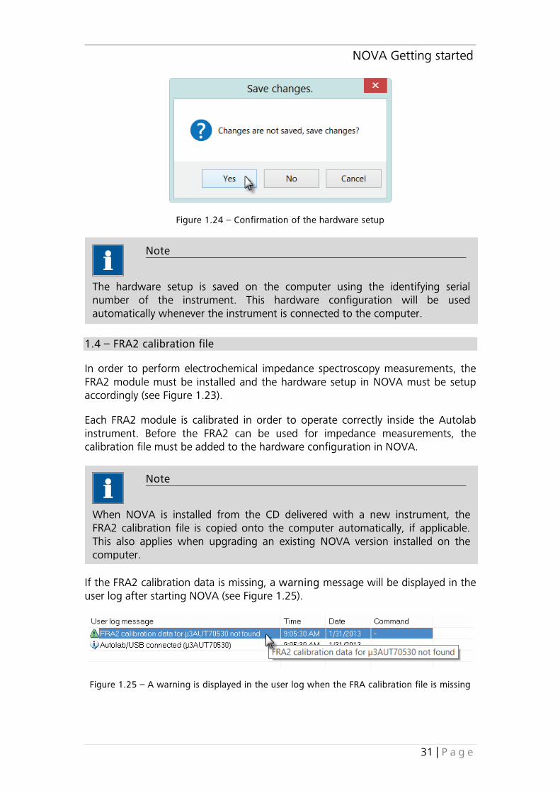
Click the OK button to close the hardware setup. You will be prompted to confirm the hardware setup (see Figure 1.24).
Note
Adjust the Power Supply Frequency according to your regional settings (50 Hz, 60 Hz).
NOVA Getting started
31 | P a g e
Figure 1.24 – Confirmation of the hardware setup
1.4 – FRA2 calibration file
In order to perform electrochemical impedance spectroscopy measurements, the FRA2 module must be installed and the hardware setup in NOVA must be setup accordingly (see Figure 1.23).
Each FRA2 module is calibrated in order to operate correctly inside the Autolab instrument. Before the FRA2 can be used for impedance measurements, the calibration file must be added to the hardware configuration in NOVA.
If the FRA2 calibration data is missing, a warning message will be displayed in the user log after starting NOVA (see Figure 1.25).
Figure 1.25 – A warning is displayed in the user log when the FRA calibration file is missing
Note
The hardware setup is saved on the computer using the identifying serial number of the instrument. This hardware configuration will be used automatically whenever the instrument is connected to the computer.
Note
When NOVA is installed from the CD delivered with a new instrument, the FRA2 calibration file is copied onto the computer automatically, if applicable. This also applies when upgrading an existing NOVA version installed on the computer.

NOVA Getting started
32 | P a g e
In this case, the FRA2 calibration file must be imported manually. This file (fra2cal.ini) can be found in two different locations:
• If the GPES/FRA software is already installed on the computer, the fra2cal.ini file can be found in the C:\autolab folder.
• Alternatively, the fra2cal.ini file can be found on the GPES/FRA 4.9 installation CD matching the serial number of the instrument7, in the D:\install\disk1 folder.
To import the FRA2 calibration file, select the Hardware setup from the Tools menu. In the Hardware setup window, click the button and locate the file fra2cal.ini (see Figure 1.26). Browse to the folder containing the calibration file and click the Open button to load the file.
Figure 1.26 – Import the FRA2 calibration file
7 The serial number of the instrument can be found on label(s) attached to the cell cables or on the back panel of the instrument.
Warning
If the fra2cal.ini file cannot be located, contact your local distributor (serial number of the instrument required).

NOVA Getting started
33 | P a g e
You will be prompted to define the type of instrument for which the fra2cal.ini file is intended (see Figure 1.27).
Figure 1.27 – Selecting the instrument type for the fra2cal.ini file
Click the OK button to confirm the selection of the instrument8 and the OK button in the Nova options window to complete the installation of the FRA2 module calibration file.
Figure 1.28 – Replacement of a previously defined fra2cal.ini file
8 See the front panel of the instrument.
Note
If a calibration file was previously imported in Nova, an overwrite warning will be displayed. Click the Yes button to confirm the replacement of the file (see Figure 1.28).

NOVA Getting started
34 | P a g e
Figure 1.29 – Adjusting the FRA offset DAC range
Note
The FRA2 calibration file is saved in the hardware setup file of the connected instrument. This calibration data will be automatically whenever the instrument is connected to the computer.
Warning
Depending of the type of FRA2 module, the FRA offset DAC range needs to be adjusted to the correct value. FRA2 modules labeled FRA2 V10 on the front panel must be set to 10V offset DAC range. FRA2 modules labeled FRA2 on the front panel must be set to 5V (see Figure 1.36). This does not apply to FRA2 modules installed in the µAutolab type III, for which this field is greyed out.
Note
Some FRA2 modules, originally fitted with a 5V range have been modified to the 10V range for special applications.

NOVA Getting started
35 | P a g e
1.5 – Diagnostics
Nova includes a diagnostics tool that can be used to test the Autolab instrument. This tool is provided as a standalone application and can be accessed from the start menu, in the Autolab group (Start menu – All programs – Autolab – Tools).
The diagnostics tool can be used to troubleshoot an instrument or perform individual tests to verify the correct operation of the instrument. Depending on the instrument type, the following items are required:
• µAutolab type II, µAutolab type III and µAutolab type III/FRA2: the standard Autolab dummy cell. For the diagnostics test, the circuit (a) is used.
• PGSTAT101 and M101 module: the internal dummy cell is used during the test, no additional items are required.
• PGSTAT204: the standard Autolab dummy cell. For the diagnostics test, the circuit (a) is used.
• Other PGSTATs: the standard Autolab dummy cell and a 50 cm BNC cable. For the diagnostics test, the circuit (a) is used. The BNC cable must be connected between the ADC164 channel 2 and the DAC164 channel 2 on the front panel of the instrument9.
9 In the case of a PGSTAT with serial number not starting with AUT7 or AUT8, connect the BNC cable between DAC channel 4 and ADC channel 4.
Warning
For the FRA2 module make sure that the FRA2 offset DAC range property is set properly in the hardware setup. For FRA2 modules, the correct value is 5 V. For FRA2.V10 modules, the correct value is 10 V. Failure to set this value properly may result in faulty data at frequencies of 25 Hz and lower (refer to front panel labels of the FRA2 module on the instrument).
Note
The PGSTAT302F must be tested in normal mode.

NOVA Getting started
36 | P a g e
The Diagnostics application supports multiple Autolab instruments. When the application starts it detects all available instruments connected to the computer (see Figure 1.30).
Figure 1.30 – The Diagnostics application automatically scans for all the connected instruments
If more than one instrument is detected, a selection menu is displayed before the Diagnostics starts (see Figure 1.31).
Figure 1.31 – A selection menu is displayed if more than one instrument is detected
The test can only be performed on a single instrument at a time. Select the instrument that needs to be tested and click the button to proceed.
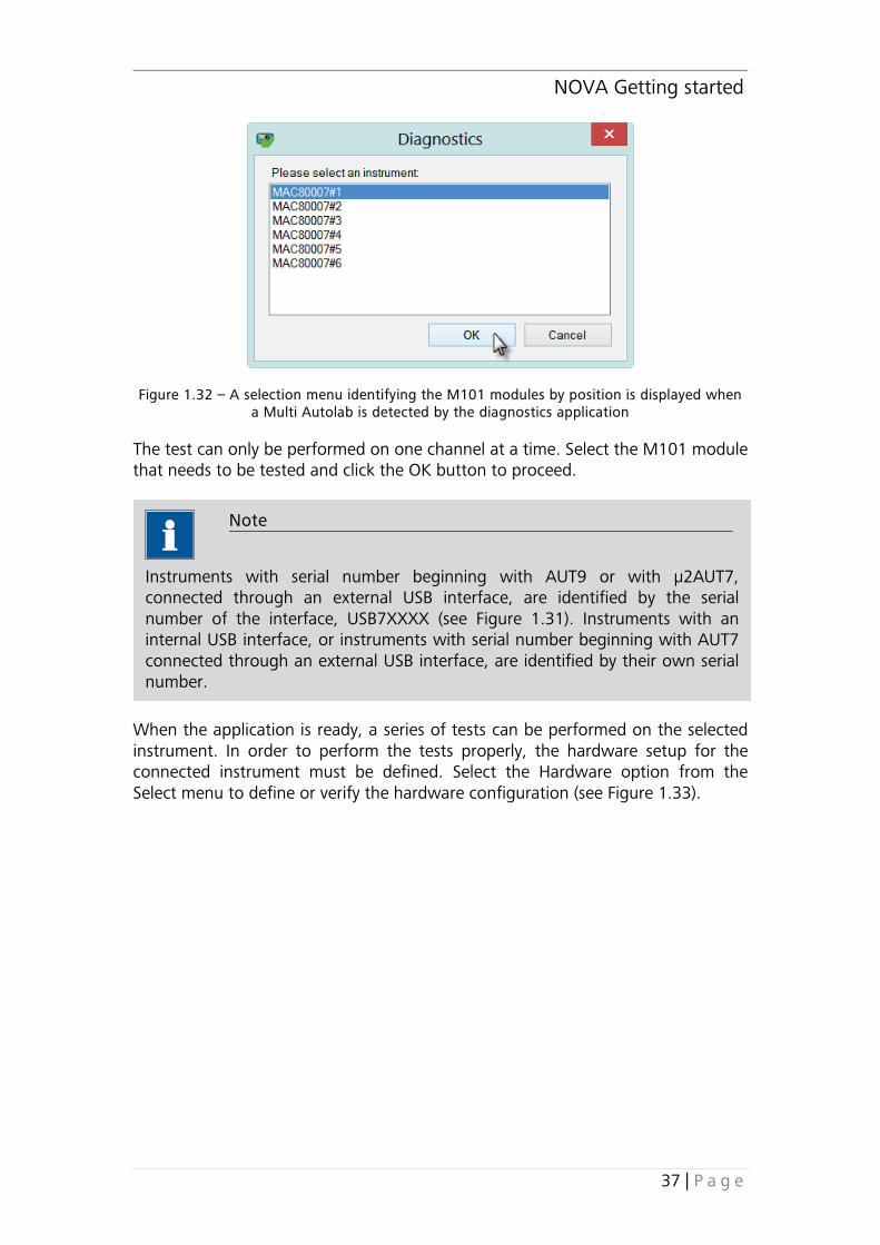
When the diagnostics application is started with a Multi Autolab connected, the application will search for the available M101 modules installed in the Multi Autolab and will list the available modules as shown in Figure 1.32.
NOVA Getting started
37 | P a g e
Figure 1.32 – A selection menu identifying the M101 modules by position is displayed when a Multi Autolab is detected by the diagnostics application
The test can only be performed on one channel at a time. Select the M101 module that needs to be tested and click the OK button to proceed.
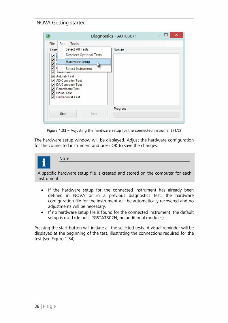
When the application is ready, a series of tests can be performed on the selected instrument. In order to perform the tests properly, the hardware setup for the connected instrument must be defined. Select the Hardware option from the Select menu to define or verify the hardware configuration (see Figure 1.33).
Note
Instruments with serial number beginning with AUT9 or with µ2AUT7, connected through an external USB interface, are identified by the serial number of the interface, USB7XXXX (see Figure 1.31). Instruments with an internal USB interface, or instruments with serial number beginning with AUT7 connected through an external USB interface, are identified by their own serial number.
NOVA Getting started
38 | P a g e
Figure 1.33 – Adjusting the hardware setup for the connected instrument (1/2)
The hardware setup window will be displayed. Adjust the hardware configuration for the connected instrument and press OK to save the changes.
• If the hardware setup for the connected instrument has already been defined in NOVA or in a previous diagnostics test, the hardware configuration file for the instrument will be automatically recovered and no adjustments will be necessary.
• If no hardware setup file is found for the connected instrument, the default setup is used (default: PGSTAT302N, no additional modules).
Pressing the start button will initiate all the selected tests. A visual reminder will be displayed at the beginning of the test, illustrating the connections required for the test (see Figure 1.34).
Note
A specific hardware setup file is created and stored on the computer for each instrument.

NOVA Getting started
39 | P a g e
Figure 1.34 – A visual reminder is shown at the beginning of the Diagnostics test
During the test, the progress will be displayed and a successful test will be indicated by a green symbol (see Figure 1.35).

NOVA Getting started
40 | P a g e
Figure 1.35 – The diagnostics report after all the tests have been performed successfully
If one or more of the tests fails, a red symbol will be used to indicate which test failed and what the problem is. Figure 1.36 shows the output of the diagnostics tool for a failed PSTAT and GSTAT test.
Figure 1.36 – A failed test will be indicated in the diagnostics tool
It is possible to print the test report or to save it as a text file by using the File menu and selecting the appropriate action (see Figure 1.37).

NOVA Getting started
41 | P a g e
Figure 1.37 – It is possible to save or print the diagnostics report
Note
At the end of the test, it is possible to perform the diagnostics test on another device, if applicable. Use the Select instrument option from the Edit menu to restart the instrument detection (see Figure 1.38). The list of available devices will be displayed after the detection process is finished (see Figure 1.30 and Figure 1.31).

NOVA Getting started
42 | P a g e
Figure 1.38 – It is possible to restart the instrument detection at the end of the test to diagnose another device
When a FI20-Integrator10 is specified in the Hardware setup (for instruments with a FI20 module or an on-board integrator), a message will be displayed at the end of the Integrator test (see Figure 1.39).
Figure 1.39 – The value of the measured Integrator calibration factor is displayed at the end of the integrator test (left: calibration factor different from stored value, right: calibration
factor unchanged)
Click OK to save the measured value in the hardware setup file of the instrument.
10 The determination of the integrator calibration factor does not replace the full test of the module. Please refer to Sections 1.6.9-1.6.11 or to the Module test document, available from the Help menu for more information on the complete test of the FI20-Integrator.

NOVA Getting started
43 | P a g e
1.5.1 – Autolab Firmware Update
For some instruments, a firmware update may be required. If this is the case of the connected instrument, a message will be displayed during the Diagnostics test (see Figure 1.40).
During Diagnostics, an update message will be displayed if the outdated firmware is detected. Clicking the Yes button when prompted will silently update the firmware (see Figure 1.40).
Figure 1.40 – An upgrade message is displayed when the outdated firmware is detected
The firmware update is permanent. The Firmware Update window will close automatically at the end of the update and the diagnostics test will continue.
Important
Do not switch off the instrument or disconnect the instrument during the firmware update since this will damage the instrument.

NOVA Getting started
44 | P a g e
1.6 – Module test in NOVA
Nova includes a number of procedures designed to verify the basic functionality of the different hardware modules installed in the instrument. These tests can be performed at any time using the Autolab dummy cell11.
These procedures are located in the Module test database located in the C:\Program Files\Metrohm Autolab\Nova 1.10\Shared DataBases\ folder. To use these procedures, define the location of the Module test folder as the Standard database, using the Database manager, available from the Tools menu (see Figure 1.41).
Figure 1.41 – Loading the Module test database
A total of 25 procedures are provided in the Module test database (see Figure 1.42).
11 Except for the Autolab PGSTAT101, the Autolab M101 module and the Autolab EQCM module.

NOVA Getting started
45 | P a g e
Figure 1.42 – The Module test procedures
The first two procedures (PGSTAT C1 calibration and PGSTAT C2 calibration) are special procedures used to determine the C1 and C2 factors required for the operation of the FRA32M or the FRA2 module in combination with the Autolab. These procedures are intended to be used under the experimental conditions described in the module installation documentation. Please refer to Section 1.6.18 for more information.
The other 23 procedures can be used at any time to test the different hardware modules installed in the instrument.
This section provides a short description of the test procedures included in the Hardware test database.
Note
Make sure that the hardware setup is defined correctly (see Section 1.3).

NOVA Getting started
46 | P a g e
1.6.1 – Test of the Autolab PGSTAT 1.6.1.1 – Test of the Autolab PGSTAT128N, 302N, 302F (normal mode), 100N, 204 and µAutolab III
This simple test is designed to verify the basic functionality of the potentiostat12. It can be used to test all the Autolab PGSTAT instruments except the Autolab PGSTAT101, the Autolab M101 potentiostat/galvanostat module13 and the PGSTAT302F in normal mode14.
Load the TestCV procedure from the Standards database, connect dummy cell (a) and press the start button (see Figure 1.43).
Figure 1.43 – The TestCV procedure requires connection to the dummy cell (a)
12 This test is also used to test earlier Autolab instruments (PGSTAT10, 20, 12, 30, 302, 100) and the µAutolabII. 13 A specific test for the PGSTAT101 and the M101 is provided (see section 1.6.1.2). 14 A specific test for the PGSTAT302F in floating mode is provided (see section 1.6.1.3).
SCE
RE
WE
CE
RE
WE(+S)(e)
WE(+S)(c)
WE(+S)(b)
WE(+S)(a)
WE(+S)(d)
DUMMY CELL2
R2
R1
R4
R3
R5
R6
C1
C4
R710kΩ
1µF
C2 1µF
C3 1µF
1µF
100Ω
100Ω
1MΩ
1MΩ
1kΩ
5kΩ

NOVA Getting started
47 | P a g e
A message will be displayed when the measurement starts (see Figure 1.44).
Figure 1.44 – A message is displayed at the beginning of the measurement
The test uses the cyclic voltammetry staircase method and performs a single potential scan starting from 0 V, between 1 V and -1V. At the end of the measurement, switch to the Analysis view and load the data for evaluation.
The data set includes three groups of data points (see Figure 1.45).
Figure 1.45 – The data obtained with the TestCV procedure
The first group, located under TestCV (Measured data) contains the measured curve and the data after baseline correction (see Figure 1.46).

NOVA Getting started
48 | P a g e
Figure 1.46 – The data points recorded during the TestCV measurement (left) and the data points after linear baseline correction (right)
The difference between the maxima observed in the residual current plot should be < 40 nA.
The second group, located under TestCV (Reference data) contains data from a reference measurement. This data can be used for comparison with the data points obtained during the test. Two reference curves are provided: the i vs E plot and the Residual plot after baseline correction.
The third group, located under Limits, contains the absolute maximum and minimum limit allowed for the residual current calculated from the measured data points.
Figure 1.47 shows an overlay of the residual current calculated from the measured data, the residual current plot provided as reference data and the absolute limits allowed for the residual current.

NOVA Getting started
49 | P a g e
Figure 1.47 – An overlay of the residual current obtained from the measured data (blue curve), the residual current from the reference data (red curve) and the absolute limits (green
lines)
1.6.1.2 – Test of the Autolab PGSTAT101 and M101
This simple test is designed to verify the basic functionality of the Autolab PGSTAT101 and the Autolab M101 potentiostat/galvanostat module15.
Load the TestCV PGSTAT101 procedure from the Standards database. This test uses the internal dummy cell of the instrument. Connect the CE and the RE electrode leads and the WE and S from the cell cable as shown in Figure 1.48 and press the start button.
15 For testing the PGSTAT302F in floating mode please refer to section 1.6.1.3. For testing all the other Autolab instruments, please refer to section 1.6.1.1.

NOVA Getting started
50 | P a g e
Figure 1.48 – The connections required for the PGSTAT101 test
A warning message, indicating that the internal dummy cell is used, will be shown during validation (see Figure 1.49). This warning is provided as a reminder and the OK button can be clicked to proceed with the measurement.
Figure 1.49 – A warning message is shown during validation
A message will be displayed when the measurement starts (see Figure 1.50).
CE
RE
SW
E

NOVA Getting started
51 | P a g e
Figure 1.50 – A message is displayed at the beginning of the measurement
The test uses the cyclic voltammetry staircase method and performs a single potential scan starting from 0 V, between 1 V and -1V. At the end of the measurement, switch to the Analysis view and load the data for evaluation.
The data set includes two groups of data points (see Figure 1.51).
Figure 1.51 – The data obtained with the TestCV PGSTAT101 procedure
The first group contains the measured data points. The other group contains data points from a reference measurement. This data can be used for comparison with the data points obtained during the test.
The measured data should be similar to the reference data provided for comparison, as shown in Figure 1.52.
NOVA Getting started
52 | P a g e
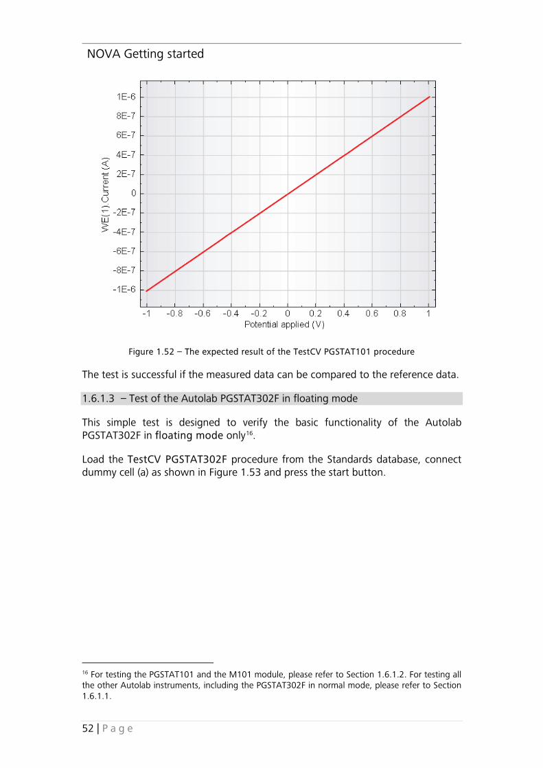
Figure 1.52 – The expected result of the TestCV PGSTAT101 procedure
The test is successful if the measured data can be compared to the reference data.
1.6.1.3 – Test of the Autolab PGSTAT302F in floating mode
This simple test is designed to verify the basic functionality of the Autolab PGSTAT302F in floating mode only16.
Load the TestCV PGSTAT302F procedure from the Standards database, connect dummy cell (a) as shown in Figure 1.53 and press the start button.
16 For testing the PGSTAT101 and the M101 module, please refer to Section 1.6.1.2. For testing all the other Autolab instruments, including the PGSTAT302F in normal mode, please refer to Section 1.6.1.1.

NOVA Getting started
53 | P a g e
Figure 1.53 – The connections to the dummy cell (a) required to test the PGSTAT302F in floating mode
A message will be displayed when the measurement starts (see Figure 1.54).
Figure 1.54 – A message is displayed at the beginning of the measurement
The test uses the cyclic voltammetry staircase method and performs a single potential scan starting from 0 V, between 1 V and -1V. At the end of the measurement, switch to the Analysis view and load the data for evaluation.
The data set includes three groups of data points (see Figure 1.55).
SWE
RE
CE
CE
RE
WE(+S)(e)
WE(+S)(c)
WE(+S)(b)
WE(+S)(a)
WE(+S)(d)
DUMMY CELL2
R2
R1
R4
R3
R5
R6
C1
C4
R710kΩ
1µF
C2 1µF
C3 1µF
1µF
100Ω
100Ω
1MΩ
1MΩ
1kΩ
5kΩ

NOVA Getting started
54 | P a g e
Figure 1.55 – The data obtained with the TestCV procedure
The first group, located under TestCV PGSTAT302F (Measured data) contains the measured curve and the data after baseline correction.
The second group, located under TestCV PGSTAT302F (Reference data) contains data from a reference measurement. This data can be used for comparison with the data points obtained during the test. Two reference curves are provided: the i vs E plot and the Residual plot after baseline correction.
The third group, located under Limits, contains the absolute maximum and minimum limit allowed for the residual current calculated from the measured data points.
Figure 1.56 shows an overlay of the residual current calculated from the measured data, the residual current plot provided as reference data and the absolute limits allowed for the residual current.

NOVA Getting started
55 | P a g e
Figure 1.56 – An overlay of the residual current obtained from the measured data (blue curve), the residual current from the reference data (red curve) and the absolute limits (green
lines)
1.6.2 – Test of the ADC750 or the ADC10M
Two procedures, TestADC750 and TestADC10M can be used to test the correct functionality of the fast sampling ADC module (ADC750 or ADC10M, respectively).
Load the TestADC750 or the TestADC10M procedure depending on the module to test from the Standards database, connect dummy cell (c) and press the start button.
A message will be displayed when the measurement starts (see Figure 1.57).
Figure 1.57 – A message is displayed at the beginning of the measurement

NOVA Getting started
56 | P a g e
The test uses the chrono amperometry high speed method and performs a total of four potential steps. At the end of the measurement, switch to the Analysis view and load the data for evaluation.
The data set includes two groups of data points (see Figure 1.58).
Figure 1.58 – The data obtained with the TestADC10M procedure
The first group, located under TestADC10M (Measured data) contains the measured current and measured potential plotted versus corrected time. The second group contains data from a reference measurement. This data can be used for comparison with the data points obtained during the test.
The measured data should be similar to the reference data provided for comparison as shown in Figure 1.59.
Note
No data points can be shown real time during measurements with the fast-sampling ADC module.
Note
The data for the TestADC750 is displayed in a similar way.
Note
Small deviation can be observed between the measured data points and the reference data because of the tolerance of the capacitance included in the dummy cell (± 5%).
NOVA Getting started
57 | P a g e
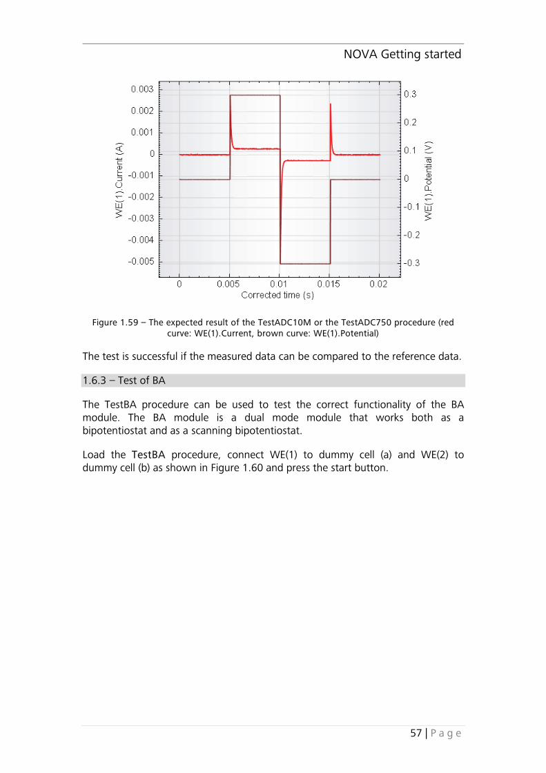
Figure 1.59 – The expected result of the TestADC10M or the TestADC750 procedure (red curve: WE(1).Current, brown curve: WE(1).Potential)
The test is successful if the measured data can be compared to the reference data.
1.6.3 – Test of BA
The TestBA procedure can be used to test the correct functionality of the BA module. The BA module is a dual mode module that works both as a bipotentiostat and as a scanning bipotentiostat.
Load the TestBA procedure, connect WE(1) to dummy cell (a) and WE(2) to dummy cell (b) as shown in Figure 1.60 and press the start button.

NOVA Getting started
58 | P a g e
Figure 1.60 – Overview of the connections to the dummy cell required for the TestBA, TestBIPOT and TestARRAY procedures
A message will be displayed when the measurement starts.
The test uses the cyclic voltammetry staircase method and performs a total of two potential scans. During the first scan, the BA is set to Bipotentiostat mode (potential of WE(2) is expressed relative to the potential of the reference electrode). During the second scan, the BA is set to scanning bipotentiostat mode (potential of WE(2) is expressed relative to the potential of WE(1)). In both measurements, the offset potential used for WE(2) is 1 V.
At the end of the measurement, switch to the Analysis view and load the data for evaluation.
The data set includes four groups of data points (see Figure 1.61).
WE2
SCE
RE
WE
CE
RE
WE(+S)(e)
WE(+S)(c)
WE(+S)(b)
WE(+S)(a)
WE(+S)(d)
DUMMY CELL2
R2
R1
R4
R3
R5
R6
C1
C4
R710kΩ
1µF
C2 1µF
C3 1µF
1µF
100Ω
100Ω
1MΩ
1MΩ
1kΩ
5kΩ
Note
Two measurements are performed during the test.

NOVA Getting started
59 | P a g e
Figure 1.61 – The data obtained with the TestBA procedure
The first two groups contain the measured data points for the WE(2).Current in Bipot mode and in Scanning Bipot mode. The other two groups contain data points for the WE(2).Current from a reference measurement. This data can be used for comparison with the data points obtained during the test.
The measured data should be similar to the reference data provided for comparison as shown in Figure 1.62.
Figure 1.62 – The expected result of the TestBA procedure (red curve: WE(2).Current (Bipot mode), brown curve: WE(2).Current (Scanning Bipot mode))
The test is successful if the measured data can be compared to the reference data.

NOVA Getting started
60 | P a g e
1.6.4 – Test of BIPOT
The TestBIPOT procedure can be used to test the correct functionality of the BIPOT module.
Load the TestBIPOT procedure, connect WE(1) to dummy cell (a) and WE(2) to dummy cell (b) as shown in Figure 1.60 and press the start button.
A message will be displayed when the measurement starts. The test uses the cyclic voltammetry staircase method and performs a single potential scan. During this scan the potential of the WE(2) is controlled with respect to the potential of the reference electrode, with a potential offset of 1 V.
At the end of the measurement, switch to the Analysis view and load the data for evaluation.
The data set includes two groups of data points (see Figure 1.63).
Figure 1.63 – The data obtained with the TestBIPOT procedure
The first group contains the measured data points. The other group contains data points for the WE(2).Current from a reference measurement. This data can be used for comparison with the data points obtained during the test.
The measured data should be similar to the reference data provided for comparison as shown in Figure 1.64.

NOVA Getting started
61 | P a g e
Figure 1.64 – The expected result of the TestBIPOT procedure
The test is successful if the measured data can be compared to the reference data.
1.6.5 – Test of ARRAY
The TestARRAY procedure can be used to test the correct functionality of the ARRAY module17.
Load the TestARRAY procedure, connect WE(1) to dummy cell (a) and WE(2) to dummy cell (b) as shown in Figure 1.60 and press the start button.
A message will be displayed when the measurement starts. The test uses the cyclic voltammetry staircase method and performs a single potential scan. During this scan the potential of the WE(2) is controlled with respect to the potential of WE(1), with a potential offset of 1 V.
At the end of the measurement, switch to the Analysis view and load the data for evaluation.
17 If the BIPOT module is equipped with a switch on the front panel of the instrument, the TestBIPOT can be used to test the bipotentiostat mode and the TestARRAY can be used to test the scanning bipotentiostat mode.

NOVA Getting started
62 | P a g e
The data set includes two groups of data points (see Figure 1.65).
Figure 1.65 – The data obtained with the TestARRAY procedure
The first group contains the measured data points. The other group contains data points for the WE(2).Current from a reference measurement. This data can be used for comparison with the data points obtained during the test.
The measured data should be similar to the reference data provided for comparison as shown in Figure 1.66.
Figure 1.66 – The expected result of the TestARRAY procedure
The test is successful if the measured data can be compared to the reference data.
1.6.6 – Test of the Booster10A and the Booster20A
The TestBooster10A and TestBooster20A procedures can be used to test the correct functionality of the Booster10A and Booster20A, respectively. Before these tests can be performed, make sure that the hardware setup is defined properly and that the Booster is installed correctly.
Load the TestBooster10A or TestBooster20A procedure depending on the type of Booster. Connect the PGSTAT and the Booster to the special booster test cell. Press the start button to begin the measurement.

NOVA Getting started
63 | P a g e
A message will be displayed when the measurement starts. The test uses the cyclic voltammetry staircase method and performs a single potential scan. During this scan the potential of the working electrode is scanning between -1 V and 1 V.
At the end of the measurement, switch to the Analysis view and load the data for evaluation.
The data set includes two groups of data points (see Figure 1.67).
Figure 1.67 – The data obtained with the TestBooster10A procedure
The first group contains the measured data points. The other group contains data points from a reference measurement. This data can be used for comparison with the data points obtained during the test.
The measured data should be similar to the reference data provided for comparison as shown in Figure 1.68.
Note
The data for the TestBooster20A is displayed in a similar way.
Note
Small deviation can be observed between the measured data points and the reference data because of the tolerance of the resistance included in the special booster test cell (± 5%).

NOVA Getting started
64 | P a g e
Figure 1.68 – The expected result of the TestBooster10A procedure (left) and the TestBooster20A procedure (right)
The test is successful if the measured data can be compared to the reference data.
1.6.7 – Test of ECD
The TestECD procedure can be used to test the correct functionality of the ECD module.
Load the TestECD procedure, connect WE(1) to dummy cell (a) and press the start button.
A message will be displayed when the measurement starts. The test uses the cyclic voltammetry staircase method and performs a single potential scan. During this scan the potential of the working electrode is scanning between -1 V and 1 V.
At the end of the measurement, switch to the Analysis view and load the data for evaluation.
The data set includes two groups of data points (see Figure 1.69).
Figure 1.69 – The data obtained with the TestECD procedure
The first group contains the measured data points. The other group contains data points from a reference measurement. This data can be used for comparison with the data points obtained during the test.
The measured data should be similar to the reference data provided for comparison as shown in Figure 1.70.

NOVA Getting started
65 | P a g e
Figure 1.70 – The expected result of the TestECD procedure
The test is successful if the measured data can be compared to the reference data.
1.6.8 – Test of ECN
The TestECN procedure can be used to test the correct functionality of the ECN module.
Load the TestECN procedure, connect the ECN cable to the --> E input of the ECN module. Connect the red plug of the ECN cable to dummy cell (a). Connect the black plug of the ECN cable to the CE connector of the dummy cell. Connect the RE, CE and S and WE from the PGSTAT to dummy cell (a) (see Figure 1.71).

NOVA Getting started
66 | P a g e
Figure 1.71 – Overview of the connections to the dummy cell required for the TestECN procedure
Press the start button to start the measurement. A message will be displayed when the measurement starts. The test uses the cyclic voltammetry staircase method and performs a single potential scan. During this scan the potential of the working electrode is scanning between -1 V and 1 V. The potential between the counter electrode and the working electrode is recorded by the ECN module.
At the end of the measurement, switch to the Analysis view and load the data for evaluation.
The data set includes two groups of data points (see Figure 1.72).
Figure 1.72 – The data obtained with the TestECN procedure
The first group contains the measured data points. The other group contains data points from a reference measurement. This data can be used for comparison with the data points obtained during the test.
The measured data should be similar to the reference data provided for comparison as shown in Figure 1.73.
WECE S
RE
CE
RE
WE(+S)(e)
WE(+S)(c)
WE(+S)(b)
WE(+S)(a)
WE(+S)(d)
DUMMY CELL2
R2
R1
R4
R3
R5
R6
C1
C4
R710kΩ
1µF
C2 1µF
C3 1µF
1µF
100Ω
100Ω
1MΩ
1MΩ
1kΩ
5kΩ
To E ECN To E ECN

NOVA Getting started
67 | P a g e
Figure 1.73 – The expected result of the TestECN procedure
The test is successful if the measured data can be compared to the reference data.
1.6.9 – Test of FI20-Filter
The TestFI20-Filter procedure can be used to test the correct functionality of the filter circuit of the FI20-Filter module.
Load the TestFI20-Filter procedure, connect dummy cell (a) and press the start button.
A message will be displayed when the measurement starts. The test uses the cyclic voltammetry staircase method and performs a single potential scan. During this scan the potential of the working electrode is scanning between -1 V and 1 V. During this measurement, the filter is switched on and a filter time-constant of 0.1 s is used.
At the end of the measurement, switch to the Analysis view and load the data for evaluation.
The data set includes two groups of data points (see Figure 1.74).
Figure 1.74 – The data obtained with the TestFI20-Filter procedure

NOVA Getting started
68 | P a g e
The first group contains the measured data points. The other group contains data points from a reference measurement. This data can be used for comparison with the data points obtained during the test.
The measured data should be similar to the reference data provided for comparison as shown in Figure 1.75.
Figure 1.75 – The expected result of the TestFI20-Filter procedure
The test is successful if the measured data can be compared to the reference data.
1.6.10 – Test of FI20-Integrator
The TestFI20-Integrator procedure can be used to test the correct functionality of the integrator circuit of the FI20-Integrator module for the Autolab PGSTAT series (except the PGSTAT101 for which a specific test is provided, see Section 1.6.11) and the µAutolab II and III.
Load the TestFI20-Integrator procedure, connect dummy cell (a) and press the start button.
Note
The FI20-Integrator needs to be properly calibrated before the test. Integrator calibration is performed in the Diagnostics application. Please refer to Section 1.5 of the Getting Started manual or the FI20 tutorial for more information.

NOVA Getting started
69 | P a g e
A message will be displayed when the measurement starts. The test uses the cyclic voltammetry current integration staircase method and performs a single potential scan. During this scan the potential of the working electrode is scanning between -1 V and 1 V. During this measurement, an integration time-constant of 0.01 s is used.
At the end of the measurement, switch to the Analysis view and load the data for evaluation.
The data set includes two groups of data points (see Figure 1.76).
Figure 1.76 – The data obtained with the TestFI20-Integrator procedure
The first group contains the measured data points. The other group contains data points from a reference measurement. This data can be used for comparison with the data points obtained during the test.
The measured data should be similar to the reference data provided for comparison as shown in Figure 1.77.
Figure 1.77 – The expected result of the TestFI20-Integrator procedure
The test is successful if the measured data can be compared to the reference data.

NOVA Getting started
70 | P a g e
1.6.11 – Test of FI20-Integrator-PGSTAT101
The TestFI20-Integrator-PGSTAT101 procedure can be used to test the correct functionality of the on-board integrator of the PGSTAT101 and the Autolab M101 potentiostat/galvanostat module.
Load the TestFI20-Integrator-PGSTAT101 procedure.
This test uses the internal dummy cell of the instrument. Connect the CE and the RE electrode leads and the WE and S from the cell cable as shown in Figure 1.78 and press the start button.
Note
The current recorded during current integration cyclic voltammetry strongly depends on the value of the capacitance included in the circuit of dummy cell (a). This capacitance has a tolerance of ± 5 %. The measured data points should therefore by qualitatively compared to the reference data provided with the test.
Note
The FI20-Integrator needs to be properly calibrated before the test. Integrator calibration is performed in the Diagnostics application. Please refer to Section 1.5 of the Getting Started manual or the FI20 tutorial for more information.
Warning
This test is designed for the PGSTAT101 and M101 only. For all the other Autolab instruments fitted with a FI20 module, please use the TestFI20-Integrator procedure (see Section 1.6.10).

NOVA Getting started
71 | P a g e
Figure 1.78 – The connections required for the TestFI20-Integrator-PGSTAT101 procedure
A warning message, indicating that the internal dummy cell is used, will be shown during validation (see Figure 1.79). This warning is provided as a reminder and the OK button can be clicked to proceed with the measurement.
Figure 1.79 – A warning is displayed at the beginning of the procedure
A message will be displayed when the measurement starts (see Figure 1.80).
CE
RE
SW
E

NOVA Getting started
72 | P a g e
Figure 1.80 – A message is displayed at the beginning of the test
The test uses the cyclic voltammetry current integration staircase method and performs a single potential scan. During this scan the potential of the working electrode is scanning between -1 V and 1 V. During this measurement, an integration time-constant of 0.01 s is used.
At the end of the measurement, switch to the Analysis view and load the data for evaluation.
The data set includes two groups of data points (see Figure 1.81).
Figure 1.81 – The data obtained with the TestFI20-Integrator-PGSTAT101 procedure
The first group contains the measured data points. The other group contains data points from a reference measurement. This data can be used for comparison with the data points obtained during the test.
The measured data should be similar to the reference data provided for comparison as shown in Figure 1.82.

NOVA Getting started
73 | P a g e
Figure 1.82 – The expected result of the TestFI20-Integrator-PGSTAT101 procedure
The test is successful if the measured data can be compared to the reference data.
1.6.12 – Test of FRA
The TestFRA procedure can be used to test the correct functionality of the FRA32M and the FRA2 module18.
18 When the FRA32M or FRA2 is installed in a PGSTAT302F, make sure that the PGSTAT302F is set to Normal mode.
Note
The current recorded during current integration cyclic voltammetry strongly depends on the value of the capacitance included in the circuit of dummy cell (a). This capacitance has a tolerance of ± 5 %. The measured data points should therefore be qualitatively compared to the reference data provided with the test.

NOVA Getting started
74 | P a g e
Load the TestFRA procedure, connect dummy cell (c) and press the start button.
A message will be displayed when the measurement starts. The test uses a potentiostatic frequency scan from 10 kHz to 0.1 Hz with a 10 mV amplitude. The frequency scan contains 50 frequencies with a logarithmic distribution. The measurement takes about four minutes to finish.
Click the OK button to continue with the measurement. During the experiment, four plots are shown in the measurement view (see Figure 1.83). Plot #1 corresponds to the Nyquist plot (-Z” vs Z’), plot #2 corresponds to the Bode plot (|Z| and -φ vs frequency), plot #3 corresponds to the resolution plot (i(resolution) vs t and E(resolution) vs t) and plot #4 corresponds to the Lissajous plot (i(AC) vs E(AC)).
Warning
For the FRA2 module make sure that the FRA2 offset DAC range property is set properly in the hardware setup. For FRA2 modules, the correct value is 5 V. For FRA2.V10 modules, the correct value is 10 V. Failure to set this value properly may result in faulty data at frequencies of 25 Hz and lower (refer to front panel labels of the FRA2 module on the instrument).
Note
Switch the measurement view to Four plots mode by pressing the button in the toolbar.

NOVA Getting started
75 | P a g e
Figure 1.83 – The measured values are displayed as a Nyquist plot (plot #1), Bode plot (plot #2), Resolution plot vs time (plot #3) and Lissajous plot (plot #4)
At the end of the measurement, the data is automatically fitted using a R(RC) equivalent circuit and the calculated values of the circuit elements are displayed in a message box (see Figure 1.84).
Figure 1.84 – The fitted values are shown in a message box at the end of the measurement (the reference values are shown in round brackets)
Reference values are shown in round brackets in the message box. The resistance values should be within ± 1% of the reference value and the capacitance value should be within ± 5% of the reference value. The calculated χ2 value should be smaller than 0.001.
Switch to the Analysis view to inspect the measured and fitted data in detail. The data set includes the measured data points and the result of an automatic fit of the impedance data with the R(RC) equivalent circuit (see Figure 1.85).

NOVA Getting started
76 | P a g e
Figure 1.85 – The data obtained with the TestFRA procedure
The value of Rs, Rp, Cdl and χ2 displayed in the explorer frame. Select the Fit and Simulation item in the data explorer and click the button located on the left hand side of the plot area to open the Equivalent Circuit Editor window (see Figure 1.86).
Figure 1.86 – Opening the results of the Fitting of the data
The results of the calculation are graphically shown in the Equivalent Circuit Editor. Select the Generate Report option from the Tools menu to display a short report table for the fitted data (see Figure 1.87). The values shown in the last column corresponds to the estimated errors on the different circuit elements, in %.

NOVA Getting started
77 | P a g e
Figure 1.87 – The Equivalent Circuit Editor window can be used to display the details of the calculation
The errors on the estimated parameters from the fitting algorithm must be smaller than 0.2 %.

NOVA Getting started
78 | P a g e
1.6.13 – Test of MUX
The TestMUX procedure can be used to test the correct functionality of the MUX module. This procedure can be used to test any type of MUX configuration.
Load the TestMUX procedure, connect Channel 1 to dummy cell (a) and Channel 2 to dummy cell (c) as shown in Figure 1.88.
Figure 1.88 – Overview of the connections to the dummy cell required for the TestMUX procedure (left: MULTI4, right: SCNR16)
Press the start button. A message will be displayed when the measurement starts. The test uses the cyclic voltammetry staircase method and performs two single potential scans. The first scan is performed on Channel 1 and the second scan is performed on Channel 2.
During each scan the potential of the working electrode is scanning between -1 V and 1 V. The recorded data points for Channel 1 are displayed on plot #1 and the data points for Channel 2 are displayed on plot #2.
At the end of the measurement, switch to the Analysis view and load the data for evaluation.
S2WE2
RE2
CE2 S1WE1
RE1
CE1
CE
RE
WE(+S)(e)
WE(+S)(c)
WE(+S)(b)
WE(+S)(a)
WE(+S)(d)
DUMMY CELL2
R2
R1
R4
R3
R5
R6
C1
C4
R710kΩ
1µF
C2 1µF
C3 1µF
1µF
100Ω
100Ω
1MΩ
1MΩ
1kΩ
5kΩ
WE2
CE
RE
WE1
CE
RE
WE(+S)(e)
WE(+S)(c)
WE(+S)(b)
WE(+S)(a)
WE(+S)(d)
DUMMY CELL2
R2
R1
R4
R3
R5
R6
C1
C4
R710kΩ
1µF
C2 1µF
C3 1µF
1µF
100Ω
100Ω
1MΩ
1MΩ
1kΩ
5kΩ
Note
Switch the measurement view to Two plots vertically tiled mode by pressing the button in the toolbar.
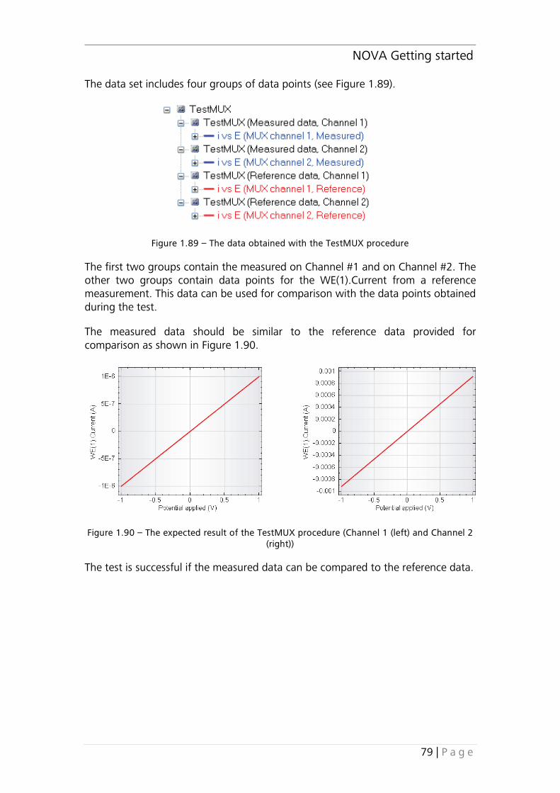
NOVA Getting started
79 | P a g e
The data set includes four groups of data points (see Figure 1.89).
Figure 1.89 – The data obtained with the TestMUX procedure
The first two groups contain the measured on Channel #1 and on Channel #2. The other two groups contain data points for the WE(1).Current from a reference measurement. This data can be used for comparison with the data points obtained during the test.
The measured data should be similar to the reference data provided for comparison as shown in Figure 1.90.
Figure 1.90 – The expected result of the TestMUX procedure (Channel 1 (left) and Channel 2 (right))
The test is successful if the measured data can be compared to the reference data.

NOVA Getting started
80 | P a g e
1.6.14 – Test of pX and pX1000
The TestpX and TestpX1000 procedures can be used to test the correct functionality of the pX and pX1000 modules, respectively. Both tests are performed on the dummy cell.
Load the TestpX or the TestpX1000 procedure depending on the module to test from the Standards database. Connect the pX/pX1000 cable to the module, on the front panel of the instrument. Connect the V+ lead from the pX/pX1000 cable (red lead) to dummy cell (a) and the V- lead from the pX/pX1000 cable (black lead) to the CE connector on the dummy cell. Connect the PGSTAT cables to dummy cell (a) (see Figure 1.91).
Figure 1.91 – Overview of the connections to the dummy cell required for the TestpX and the TestpX1000
Press the start button to start the measurement.
A message will be displayed when the measurement starts. The test uses the cyclic voltammetry staircase method and performs a single potential scan. During this scan the potential of the working electrode is scanning between -1 V and 1 V. The potential between the counter electrode and the working electrode is recorded by the pX/pX1000 module.
At the end of the measurement, switch to the Analysis view and load the data for evaluation.
WECE S
RE
CE
RE
WE(+S)(e)
WE(+S)(c)
WE(+S)(b)
WE(+S)(a)
WE(+S)(d)
DUMMY CELL2
R2
R1
R4
R3
R5
R6
C1
C4
R710kΩ
1µF
C2 1µF
C3 1µF
1µF
100Ω
100Ω
1MΩ
1MΩ
1kΩ
5kΩ
To pX1000 module To pX1000 module
V+V-
Warning
During the TestpX procedure, designed to verify the functionality of the pX module, make sure that the 50 Ohm resistor BNC shunt is NOT connected to the G BNC input on the front panel of the pX module.

NOVA Getting started
81 | P a g e
The data set includes two groups of data points (see Figure 1.92).
Figure 1.92 – The data obtained with the TestpX/TestpX1000 procedure
The first group contains the measured data points. The other group contains data points from a reference measurement. This data can be used for comparison with the data points obtained during the test.
The measured data should be similar to the reference data provided for comparison as shown in Figure 1.93.
Figure 1.93 – The expected result of the TestpX or the TestpX1000 procedure
The test is successful if the measured data can be compared to the reference data.
Note
The data for the TestpX is displayed in a similar way.

NOVA Getting started
82 | P a g e
1.6.15 – Test of the SCANGEN or the SCAN250
Two procedures, TestSCANGEN and TestSCAN250 can be used to test the correct functionality of the linear scan generator module (SCANGEN or SCAN250, respectively).
Load the TestSCANGEN or the TestSCAN250 procedure depending on the module to test from the Standards database, connect dummy cell (a) and press the start button.
A message will be displayed when the measurement starts.
The test uses the cyclic voltammetry linear scan method and performs a potential scan starting from 0 V, between an upper vertex potential of 1 V and a lower vertex potential of -1 V. After the first potential scan, the measurement stops at the upper vertex potential, 1 V. At the end of the measurement, switch to the Analysis view and load the data for evaluation.
The data set includes two groups of data points (see Figure 1.94).
Figure 1.94 – The data obtained with the TestSCAN250 procedure
The first group, located under TestSCAN250 (Measured data) contains the measured current plotted versus the measured potential. The second group contains data from a reference measurement. This data can be used for comparison with the data points obtained during the test.
The measured data should be similar to the reference data provided for comparison as shown in Figure 1.95.
Note
The data for the TestSCANGEN is displayed in a similar way.

NOVA Getting started
83 | P a g e
Figure 1.95 - The expected result of the TestSCAN250 or the TestSCANGEN procedure
The test is successful if the measured data can be compared to the reference data.
1.6.16 – Test of the SCANGEN or the SCAN250 in combination with the ACD750 or the ADC10M
The TestADC/SCAN procedure can be used to test the correct functionality of the linear scan generator module (SCANGEN or SCAN250) in combination with the fast sampling ADC module (ADC750 or ADC10M) for high speed linear scan cyclic voltammetry measurements.
Load the TestADC/SCAN procedure, connect dummy cell (a) and press the start button.
A message will be displayed when the measurement starts.
Note
the current recorded during a measurement with the SCANGEN or the SCAN250 module strongly depends on the value of the capacitance included in the circuit of dummy cell (a). This capacitance has a tolerance of ± 5 %. The measured data points should therefore be qualitatively compared to the reference data provided with the test.

NOVA Getting started
84 | P a g e
The test uses the cyclic voltammetry linear scan high speed method and performs a potential scan starting from 0 V, between an upper vertex potential of 1 V and a lower vertex potential of -1 V. After the first potential scan, the measurement stops at the upper vertex potential, 1 V at 100 V/s. At the end of the measurement, switch to the Analysis view and load the data for evaluation.
The data set includes two groups of data points (see Figure 1.96).
Figure 1.96 – The data obtained with the TestADC/SCAN procedure
The first group, located under TestADC/SCAN (Measured data) contains the measured current plotted versus the measured potential. The second group contains data from a reference measurement. This data can be used for comparison with the data points obtained during the test.
Note
No data points can be shown real time during measurements with the fast-sampling ADC module.

NOVA Getting started
85 | P a g e
The measured data should be similar to the reference data provided for comparison as shown in Figure 1.97.
Figure 1.97 – The expected result of the TestADC/SCAN procedure
The test is successful if the measured data can be compared to the reference data.
Note
The current recorded during a measurement during the TestADC/SCAN procedure strongly depends on the value of the capacitance included in the circuit of dummy cell (a). This capacitance has a tolerance of ± 5 %. The measured data points should therefore be qualitatively compared to the reference data provided with the test.

NOVA Getting started
86 | P a g e
1.6.17 – Test of the EQCM
The TestEQCM procedure can be used to test the correct functionality of the filter circuit of the EQCM.
Load the TestEQCM procedure and insert a 6 MHz EQCM crystal in the EQCM cell. Fill the cell with ca. 2 ml of water and check for leakage. Connect the cell to the EQCM oscillator and the oscillator to the Autolab PGSTAT using the provided cable. Leave the cell connectors from the PGSTAT disconnected. Please refer to the EQCM user manual for more information.
Press the start button to start the measurement. Two messages will be displayed when the measurement starts (see Figure 1.98).
Figure 1.98 – Two messages are displayed at the beginning of the measurement
When the second message appears, verify that the LED on the EQCM oscillator box is ON (red or green).
Click OK to continue. The Determine EQCM zero frequency window will appear (see Figure 1.99).
Warning
This procedure cannot be performed on the dummy cell and it requires about 2 ml of water.
Warning
Wait 15 minutes for the EQCM to warm up.

NOVA Getting started
87 | P a g e
Figure 1.99 – The determine EQCM zero frequency window can be used to adjust the driving force
Using the provided adjustment tool, rotate the trimmer on the EQCM oscillator in order to minimize the driving force (refer to the EQCM user manual for more information).
When the driving force has been properly minimized, the LED on the EQCM oscillator must be green. Click the button in the Determine EQCM zero frequency window to zero the value of the EQCM(1).∆Frequency signal.
After minimizing the ∆Frequency signal click the OK button to proceed with the measurement. The procedure records the three signals provided by the EQCM module during ten seconds. The EQCM(1).∆Frequency and EQCM(1).Temperature signals are shown on plot #1 and the EQCM(1).Driving force signal is shown on plot #2 (see Figure 1.100).

NOVA Getting started
88 | P a g e
Figure 1.100 – The data recorded during the TestEQCM procedure
At the end of the measurement, a message is displayed, providing qualitative validation criteria for the measured data (see Figure 1.101).
Figure 1.101 – A message is displayed at the end of the measurement
Switch to the Analysis view and load the data for evaluation. The data set includes two groups of data points (see Figure 1.102).
Note
Switch the measurement view to Two plots vertically tiled mode by pressing the button in the toolbar.

NOVA Getting started
89 | P a g e
Figure 1.102 – The data obtained with the TestEQCM procedure
The first group contains the measured data points. The other group contains data points from a reference measurement. This data can be used for comparison with the data points obtained during the test.
The EQCM measurements depend on the temperature and the crystal used during the experiment. Comparison with the provided reference data points should be performed qualitatively.
1.6.18 – Determination of the C1 and C2 factors of the Autolab
When the FRA32M or FRA2 module is used in combination with the Autolab19, the C1 and C2 factors need to be determined. These factors can be determined with the following procedures, included in the Module test database:
• PGSTAT C1 calibration • PGSTAT C2 calibration
These procedures can be used in combination with the Autolab dummy cell.
19 When the FRA32M or FRA2 is installed in a PGSTAT302F, make sure that the PGSTAT302F is set to Normal mode.
Note
The C1 and C2 are predetermined when FRA32M or FRA2 module is preinstalled. The C1 and C2 factors must be determined experimentally when a FRA32M or FRA2 module is installed into an existing instrument. This determination must only be carried out upon installation of the module.
Note
The C1 and C2 determination in not required for the M101 and the PGSTAT204.
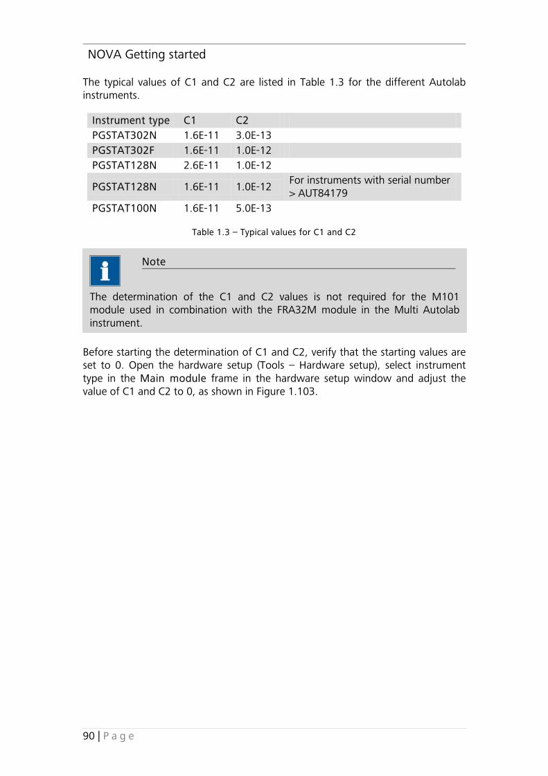
NOVA Getting started
90 | P a g e
The typical values of C1 and C2 are listed in Table 1.3 for the different Autolab instruments.
Instrument type C1 C2 PGSTAT302N 1.6E-11 3.0E-13 PGSTAT302F 1.6E-11 1.0E-12 PGSTAT128N 2.6E-11 1.0E-12
PGSTAT128N 1.6E-11 1.0E-12 For instruments with serial number > AUT84179
PGSTAT100N 1.6E-11 5.0E-13
Table 1.3 – Typical values for C1 and C2
Before starting the determination of C1 and C2, verify that the starting values are set to 0. Open the hardware setup (Tools – Hardware setup), select instrument type in the Main module frame in the hardware setup window and adjust the value of C1 and C2 to 0, as shown in Figure 1.103.
Note
The determination of the C1 and C2 values is not required for the M101 module used in combination with the FRA32M module in the Multi Autolab instrument.

NOVA Getting started
91 | P a g e
Figure 1.103 – The value of C1 and C2 must be set to 0 before starting the measurements
The determination of C1 and C2 requires the following items:
• Autolab Dummy cell • Faraday cage20
1.6.18.1 – Determination of C1
Follow the steps described in this section to determine the value of the C1 parameter.
1. Start the Nova software. 2. Load the procedure PGSTAT C1 calibration from the Module test database. 3. Connect the Autolab Dummy cell as shown in Figure 1.104. Connect the
ground lead from the PGSTAT to the Faraday cage.
20 Please contact your Autolab distributor if you need assistance.
Note
Do not connect the ground lead from the PGSTAT to the Dummy cell. Place the dummy cell in the Faraday cage.

NOVA Getting started
92 | P a g e
Figure 1.104 – Overview of the connections required for the determination of C1
4. Start the measurement and wait until it has been finished. Ignore the warning displayed during the procedure validation (see Figure 1.105).
Figure 1.105 – Ignore the warning shown during the validation of the procedure
5. A reminder message is shown at the beginning of the measurement (see Figure 1.106).
WE S
CE
RE
CE
RE
WE(+S)(e)
WE(+S)(c)
WE(+S)(b)
WE(+S)(a)
WE(+S)(d)
DUMMY CELL2
R2
R1
R4
R3
R5
R6
C1
C4
R710kΩ
1µF
C2 1µF
C3 1µF
1µF
100Ω
100Ω
1MΩ
1MΩ
1kΩ
5kΩ

NOVA Getting started
93 | P a g e
Figure 1.106 – A reminder message is shown at the beginning of the measurement
6. During the measurement, the measured data will be plotted as a Bode plot should be similar to the example shown in Figure 1.107.
Figure 1.107 – Typical Bode plot obtained during the C1 calibration
7. The data is automatically fitted and the results of the fitting are reported in a Message box at the end of the measurement (see Figure 1.108).

NOVA Getting started
94 | P a g e
Figure 1.108 – The experimentally determined value of C1 is reported in a Message box at the end of the measurement
8. Open the Hardware setup of Nova (Tools – Hardware setup). Select the instrument type in the Main Module frame in the hardware setup window and adjust the value of C1 to the value reported in the Message box (see Figure 1.109).
Figure 1.109 – Change the value of C1 to the value reported in the Message box
9. Click OK to save the changes and wait for the Autolab to be reinitialized using the updated Hardware setup.
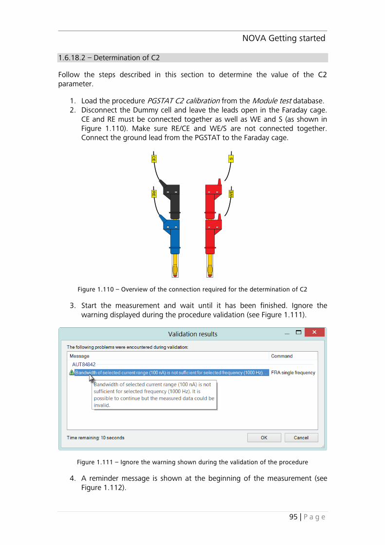
NOVA Getting started
95 | P a g e
1.6.18.2 – Determination of C2
Follow the steps described in this section to determine the value of the C2 parameter.
1. Load the procedure PGSTAT C2 calibration from the Module test database. 2. Disconnect the Dummy cell and leave the leads open in the Faraday cage.
CE and RE must be connected together as well as WE and S (as shown in Figure 1.110). Make sure RE/CE and WE/S are not connected together. Connect the ground lead from the PGSTAT to the Faraday cage.
Figure 1.110 – Overview of the connection required for the determination of C2
3. Start the measurement and wait until it has been finished. Ignore the warning displayed during the procedure validation (see Figure 1.111).
Figure 1.111 – Ignore the warning shown during the validation of the procedure
4. A reminder message is shown at the beginning of the measurement (see Figure 1.112).
CE
RE
SW
E

NOVA Getting started
96 | P a g e
Figure 1.112 – A reminder message is shown at the beginning of the measurement
5. During the measurement, the measured data will be plotted as a Bode plot should be similar to the example shown in Figure 1.113.
Figure 1.113 – Typical Bode plot obtained during the C2 calibration
6. The data is automatically fitted and the results of the fitting are reported in a Message box at the end of the measurement (see Figure 1.114).

NOVA Getting started
97 | P a g e
Figure 1.114 – The experimentally determined value of C2 is reported in a Message box at the end of the measurement
7. Open the Hardware setup of Nova (Tools – Hardware setup). Select the instrument type in the Main Module frame in the hardware setup window and adjust the value of C2 to the value reported in the Message box (see Figure 1.115).
Figure 1.115 – Change the value of C2 to the value reported in the Message box
8. Click OK to save the changes and wait for the Autolab to be reinitialized using the updated Hardware setup.

NOVA Getting started
98 | P a g e

NOVA Getting started
99 | P a g e
Nova Getting started
The aim of the NOVA Getting started is to give new users a feel of the main features of the software as well as to introduce them to its mechanics. It is also intended to test the installation of the software. The example illustrated in this section will be presented without a specific clarification for each instruction or command. This chapter is meant to be used as a walkthrough for first time users. All of the aspects of the software are discussed in more detail in the User Manual. The document can be accessed in Nova by pressing the F1 key or through the Help menu.
2 – A typical Nova measurement
A typical Nova measurement starts with a procedure. This procedure must be selected, modified if necessary and executed. Nova will run through the instructions of the procedure and carry them out sequentially. While this happens, the collected data points will be displayed in real time. At the end of the measurement the data points will be available for further analysis.
For this quick start the Autolab is used in conjunction with the dummy cell.
2.1 – Starting up the software (installation required, see Chapter 1)
Nova can be started by double clicking the Nova shortcut on the computer desktop. If an Autolab is already connected to the computer through the USB connection and turned on, the software will automatically identify the instrument and upload the required control software.
If no instrument is connected after starting Nova, connecting the Autolab to the computer using the USB and turning it on will trigger the initialization process automatically (see Chapter 1 for further details on the USB communication with the instrument).
By default, Nova will start in the Setup view. The Setup view is one of the four views the user can select while operating Nova. The other three are the Measurement view (used to display the data in real time during a measurement),
Note
GPES users are used to start a measurement by selecting a pre-defined method from a list of available techniques. Nova is designed to perform complex measurements, seamlessly switching from one electrochemical method to another in a single procedure (see Chapter 2 of the User manual for further information). Therefore the electrochemical method selection becomes obsolete (ready to use template procedures are included, see Chapter 3 for more information).

NOVA Getting started
100 | P a g e
the Analysis view (used to perform data analysis) and the Multi Autolab view (used to control the Multi Autolab or more than one instrument at the same time).
The Setup view contains several areas (also called frames). Figure 2.1 shows an overview of the Setup view.
Figure 2.1 – Overview of the Setup view of Nova
More information regarding the Setup view of Nova can be found in Chapter 2 of the User Manual.
The procedure browser frame displays a number of available procedures, in the Autolab group. Figure 2.2 shows a more detailed view of the Setup view.
Toolbar
Procedure editor frame
User logStart / Stop button
Procedure & Command browser
Quick access toolbar

NOVA Getting started
101 | P a g e
Figure 2.2 – Details of the Setup view
The procedures visible in the Autolab group in the browser are standard factory procedures. These procedures are always visible and cannot be changed or removed.
2.2 – Running cyclic voltammetry on the dummy cell
The purpose of this quick start is to perform staircase cyclic voltammetry on the Autolab dummy cell. In the example discussed below, the dummy cell (c) is used. The cell cables should therefore be connected to the dummy cell as displayed in Figure 2.3.
Note
The actual number of procedures listed in the Autolab group of procedures in the Setup view depends on the active profile. By default, the Cyclic voltammetry potentiostatic procedure should be visible in this group, unless it has been hidden on purpose. Please refer to the User manual for more information on the use of profiles in Nova.

NOVA Getting started
102 | P a g e
Figure 2.3 – Dummy cell connections
2.2.1 – Setting up the experiment
To perform a cyclic voltammetry experiment, the default Cyclic voltammetry potentiostatic procedure must be loaded into the Procedure editor. Right clicking the Cyclic voltammetry potentiostatic procedure in the browser brings up a context menu, displaying the Open for editing option (see Figure 2.4).
Figure 2.4 – Loading a procedure in the Editor frame (part 1)
S
CE
RE
WE
CE
RE
WE(+S)(e)
WE(+S)(c)
WE(+S)(b)
WE(+S)(a)
WE(+S)(d)
DUMMY CELL2
R2
R1
R4
R3
R5
R6
C1
C4
R710kΩ
1µF
C2 1µF
C3 1µF
1µF
100Ω
100Ω
1MΩ
1MΩ
1kΩ
5kΩ
Note
The PGSTAT101 is not equipped with the Autolab dummy cell. An optional external dummy cell can be obtained (Contact your Autolab distributor for more information). For the PGSTAT101, use the procedure TestCV PGSTAT101 available in the Module test database (Refer to the Module test with Nova document, available from the Help – Tutorials menu).

NOVA Getting started
103 | P a g e
Clicking this instruction will load the procedure in the editor frame. The name of procedure will change from New procedure to Cyclic voltammetry potentiostatic. A series of commands will be displayed under the Cyclic voltammetry potentiostatic procedure in the editor frame (see Figure 2.5).
These commands form the procedure and will be executed sequentially when the procedure is started.
Figure 2.5 – Loading a procedure in the Editor frame (part 2)
Once the procedure is loaded in the procedure editor frame, it can be executed. This procedure will perform a single potential scan, between -1 V and 1 V on the dummy cell, starting at a potential of 0 V, with a scan rate of 100 mV/s.
When the procedure is loaded in the procedure editor frame it can be modified and started. It is convenient to name each experiment in a unique way, for bookkeeping purposes. To change the name of the cyclic voltammetry potentiostatic procedure to a custom name, click the cyclic voltammetry potentiostatic name in the procedure editor and change it to Quick start Cyclic voltammetry (see Figure 2.6).
Note
In Nova, a procedure is defined as the combination of a signal sampler and a series of commands. The signal sampler defines which signals (current, potential, time, pH, …) will be sampled during the measurement and the commands define how these signals will be sampled.

NOVA Getting started
104 | P a g e
Figure 2.6 – Editing the procedure name
After the title has been edited, validate with the Enter key and save the procedure, using the File menu – Save procedure as New (see Figure 2.7).
Figure 2.7 – Save the procedure
The procedure will be added to the My procedures database (see Figure 2.8).

NOVA Getting started
105 | P a g e
Figure 2.8 – Adding the quick start cyclic voltammetry procedure
The procedure can now be started. Click the Start button located at the bottom of the screen to begin the experiment. The procedure is first validated, which can take a few seconds depending on the amount of commands in the procedure. If no errors are detected, the measurement starts. The software will automatically switch to the Measurement view where the measured data points are displayed in real time.
You can also switch to the Measurement view at any time by clicking the measurement view button in the toolbar (see Figure 2.9).
Figure 2.9 – Switching from the setup view to the measurement view

NOVA Getting started
106 | P a g e
2.2.2 – Viewing the measured data
The measurement view displays the measured data in real time. The default display settings for a cyclic voltammetry experiment are the potential (Potential applied) on the X-axis and the measured current on the Y-axis (WE(1).Current). The scale of the plot is automatically adjusted during the measurement.
When the measurement is running, the start button is replaced by a stop button that can be pressed to abort the experiment. Figure 2.10 shows the measurement view during the Quick start experiment.
Figure 2.10 – The Measurement view
It is possible, at any time, to pick the Autolab display option from the View menu (or to press the F10 shortcut key), as shown in Figure 2.11.
Toolbar
Measurement frame
User logStart / Stop button
Parameter editor
Quick access toolbar
Procedure progress

NOVA Getting started
107 | P a g e
Figure 2.11 – Select the Autolab display option in the View menu or use the dedicated button in the toolbar to show or hide the Autolab display window
Figure 2.12 shows the Autolab display during the measurement.
Figure 2.12 – The Autolab display

NOVA Getting started
108 | P a g e
The Autolab display provides real-time information about the sampled signals and the hardware settings and provides additional controls, like the button, which can be used to reverse the scan direction21.
The procedure used in this quick start guide performs a single scan on the dummy cell. When the scan is finished, the stop button becomes a start button again, indicating that Nova is ready to perform a new measurement.
At the end of the measurement, the User log can be updated, depending on the events that occurred during the measurement. For example, if a current overload occurred during the experiment, a message will be shown in the log (see Figure 2.13).
Figure 2.13 – The User log is automatically updated at the end of the experiment
Although the measurement view displays the measured data during and after the experiment, it is not meant for data analysis. Data analysis is performed in the dedicated analysis view. Switching to the analysis view can be done by clicking the corresponding button on the toolbar (see Figure 2.14).
Figure 2.14 – Switching from the measurement view to the analysis view
2.2.3 – Analyzing the measured data
The analysis view is used to manage experimental data and perform data analysis. Figure 2.15 shows the default layout.
21 Please refer to the Cyclic voltammetry tutorial, available from the Help – Tutorials menu, for more information.

NOVA Getting started
109 | P a g e
Figure 2.15 – The analysis view
The analysis view has several noteworthy features, the most important of which is the database. Every measurement is stored in the database automatically. Each entry of the database corresponds to a measurement and is logged together with the time and date, as well as a Remarks field and the serial number of the instrument used in the experiment. An additional field, Instrument description can be used to provide a description of the instrument (see Figure 2.16).
Figure 2.16 – Database entries are logged by Procedure name, Time stamp, Remarks, Instrument and Instrument description
The database consists of one single folder. However, if required, a specific entry of the database can be exported as a single file22.
22 Please refer to the User Manual for more information.
Toolbar
Database frame
User logStart / Stop button
Plot area
Data explorer frame
Analysis frame
Quick access toolbar

NOVA Getting started
110 | P a g e
The analysis view features a dedicated toolbar (see Figure 2.17).
Figure 2.17 – The analysis view toolbar (highlighted)
To view and analyze the data from a measurement, the corresponding entry of the database has to be loaded in the Data explorer frame.
Double click the Quick start Cyclic voltammetry entry of your database to load it in the data explorer frame. The database entry will appear in this frame as shown in Figure 2.18.
Figure 2.18 – Loading the measured data in the data explorer
Once the data from the database has been loaded into the data explorer frame, it is available for data analysis. To view the data, click the blue i vs E item in the data explorer. The measured data will be displayed using the default settings, i.e., plotting the Potential applied on the X-axis and the measured current, WE(1).Current on the Y-axis. The measured data should be displayed in the data analysis frame like in Figure 2.19.

NOVA Getting started
111 | P a g e
Figure 2.19 – Displaying the measured data in the analysis view
The final part of this quick start guide will illustrate some of the features of the analysis view. More information can be found in Chapter 4 of the User Manual.
During this experiment, the Autolab instrument recorded values for time, current and potential. These experimental values are known in Nova as Signals. These signals can be used in any combination to control the way the data is plotted.
Click the symbol next to the blue i vs E line in the data explorer frame to reveal the signals currently used for this plot (see Figure 2.20).
Figure 2.20 – Expanding the Signal set line in the data explorer frame
Figure 2.20 shows that for the current plot, the Potential applied signal is used for the X-axis and the WE(1).Current signal is used for the Y-axis. The WE(1).Current signal used for the Z-axis is not relevant for a 2D plot.
It might be useful to show the applied potential (on the Y-axis) as a function of time (on the X-axis). This can be easily done within the analysis view by right clicking the active setting for the X-axis (the WE(1).Potential applied) in the data explorer frame and replacing it by the time. The same can be done to change the signal plotted on the Y-axis from the measured WE(1).Current to the WE(1).Potential (see Figure 2.21).

NOVA Getting started
112 | P a g e
Figure 2.21 – Changing the plot settings
After changing these settings, the plot should be similar to Figure 2.22.
Figure 2.22 – Plotting the applied potential as a function of time
The familiar saw-tooth profile of a cyclic voltammogram can be easily recognized.
Nova also provides a 3D plot engine. To switch to a 3D plot, click the corresponding button of the data analysis view toolbar (see Figure 2.23).
Figure 2.23 – Showing the data in 3D
The 3D plot displays time, current, and potential on the same plot (use the WE(1).Current as the Signal for the Z-axis). This plot can be turned and rotated by

NOVA Getting started
113 | P a g e
clicking the graph and moving the mouse around while holding the left button (see Figure 2.24).
Figure 2.24 – Spinning the 3D graph around
Feel free to try to change the plot, either in the 2D or the 3D view. We recommend that you take the time to get familiar with the Nova basics before exploring the rest of the manual for more information.
Note
While holding the left mouse button, the mouse pointer changes to the pointer highlighted in Figure 2.24.

NOVA Getting started
114 | P a g e
2.2.4 – Using the data grid
A very important feature of Nova is the Data grid and its functionality. During a measurement, several signals are sampled and are stored in the database when the measurement is completed. These signals are then available in the analysis view for plotting purposes, as shown in the previous section.
For the standard Cyclic voltammetry potentiostatic measurement, these signals are:
• Potential applied • WE(1).Current • WE(1).Potential • Scan • Time • Index
The data grid provides an overview of all the signals. To access the data grid, click the corresponding button, , in the toolbar (see Figure 2.25).
Figure 2.25 – Selecting the data grid
The data grid displays all the values of each signal that was recorded during the measurement. Scrolling down the list allows you to inspect all the data points (see Figure 2.26).
Figure 2.26 – The data grid displays the values of the signals

NOVA Getting started
115 | P a g e
Using the data grid, it is possible to export the measured data points to other software’s for data analysis (Excel, Origin, SigmaPlot, …). This can be done by right-clicking the data grid and by choosing the Export ASCII data option from the context menu (see Figure 2.27).
Figure 2.27 – Exporting the data to ASCII or Excel
It is also possible to create new signals based on calculations performed on the existing signals. For example, it can be useful to calculate the logarithm of the measured current.
The data grid can be used like a spreadsheet. It comes with a signal calculator which can be used to create a new signal based on an existing signal and a mathematical operation.
To create a new signal, click the CV staircase item in the data explorer frame and select the Calculate signal tool from the quick access toolbar by clicking the button (see Figure 2.28).
Figure 2.28 – Adding a calculate signal to the CV staircase

NOVA Getting started
116 | P a g e
Alternatively, it is also possible to click the button located in the toolbar in the frame on the right-hand side of the data grid (see Figure 2.29).
Figure 2.29 – Opening the Calculate signal tool
The Calculate signal window will be displayed (see Figure 2.30).
Figure 2.30 – The Calculate signal window

NOVA Getting started
117 | P a g e
The calculate signal window works as an electrochemical calculator. It has several fields which are used to create a new signal:
• Name: this is the name of the new signal (a name is mandatory) • Single value: this checkbox can be used to force the calculate signal to
return a single value • Unit: the unit of the new signal • Expression: this is the mathematical expression used to calculate the new
signal • Parameters: a list of identified parameters used in the expression • Functions: a list of common mathematical functions that can be used to
calculate the new signal • Trigonometric functions: a list of common trigonometric functions • Signals: this is a list of the available signals in the data set
As an example, we are going to calculate the logarithm of the current in order to create a Tafel plot.
In the calculate signal window, type log(i) as a name to identify the new signal. Then, scroll down the list of functions to locate the 10LOG function and double click it to add it to the expression builder (see Figure 2.31).

NOVA Getting started
118 | P a g e
Figure 2.31 – Creating the log(i) signal – part 1: Defining the expression
Next, double click the ABS function, located under the 10LOG function, in order to add it to the expression. Finally, in the expression, change the [parameter1] text to i and click the parameters frame in the expression builder. The expression builder will identify the parameter, i, as the only parameter of the expression. This parameter will be displayed in the Parameters frame (see Figure 2.32).

NOVA Getting started
119 | P a g e
Figure 2.32 – Creating the log(i) signal – part 2: Identifying the parameters of the expression
The final step in the expression building process consists in linking the parameter(s) of the expression to existing signal(s). Expand the CV staircase list of available signals and double click the WE(1).Current signal to link it to the parameter i (see Figure 2.33).

NOVA Getting started
120 | P a g e
Figure 2.33 – Creating the log(i) signal – part 3: Linking the parameters of the expression to the available signals
The linked parameter will be displayed between brackets next to the name of the signal. The name of the signal will be displayed in red, indicating that it is linked to a parameter (see Figure 2.34).
Figure 2.34 – A detailed view of the expression builder

NOVA Getting started
121 | P a g e
Click the OK button to finish the calculation of the new signal. The contents of the data grid will be updated indicating that the new signal has been added to the list of available signals (see Figure 2.35). The expression used to calculate this signal is displayed in the calculation frame.
Figure 2.35 – The log(i) signal added to the data grid
The newly created log(i) signal can now be used as any other signal to plot the data either in 2D or 3D. Switch to the 2D plot by clicking the button in the toolbar. Set the plot settings for the X-axis to WE(1).Potential applied and for the Y-axis to log(i) as shown in Figure 2.36.
Figure 2.36 – Changing the plot settings to create the Tafel plot
Note
The log(i) has been added to the list of signals available using the right click menu.

NOVA Getting started
122 | P a g e
2.2.5 – Saving to the database
In Nova, it is possible to save the changes in the database at any time. This allows you to keep all the modifications on a given data set, as well as the results of data analysis tools or additions to the data. To update a database entry, click the located in the analysis toolbar (see Figure 2.37).
Figure 2.37 – Saving the modifications in the data base
Note
Saving the changes to the database in this case adds the log(i) signal to the data set as well as the plot settings (Tafel plot).
Note
We advise to go through the User Manual, chapter by chapter, since it provides in-depth information on procedures setup, measurements and data analysis. Alternatively, you could skip to chapter 4 of the User Manual, which explores the Data analysis features of Nova in detail to further practice on the dummy cell data obtained in the course of this quick start.

NOVA Getting started
123 | P a g e
Autolab procedures
Nova comes with a series of factory standard procedures, located in the Autolab group, that are available to every user and are intended both as examples and as simple measurement procedures.
This chapter provides an overview of the available factory standard procedures.
3 – The Autolab procedures group
The Autolab procedures group, located in the procedure browser frame contains a series of factory standard procedures. These procedures are intended to perform simple measurements and can be used for routine experiments or as templates for more elaborate procedures. The current version of Nova provides 26 Factory standard procedures (see Figure 3.1).
Figure 3.1 – The Autolab procedures group in the Procedure browser frame

NOVA Getting started
124 | P a g e
The available procedures are:
• Cyclic voltammetry potentiostatic • Cyclic voltammetry galvanostatic • Cyclic voltammetry current integration23 • Cyclic voltammetry linear scan24 • Cyclic voltammetry linear scan high speed24, 25 • Linear sweep voltammetry potentiostatic • Linear sweep voltammetry galvanostatic • Linear polarization • Hydrodynamic linear sweep26 • Differential pulse voltammetry27 • Square wave voltammetry27 • Sampled DC polarography27 • Chrono amperometry (∆t > 1 ms) • Chrono potentiometry (∆t > 1 ms) • Chrono amperometry fast • Chrono potentiometry fast • Chrono coulometry fast23 • Chrono amperometry high speed25 • Chrono potentiometry high speed25 • Chrono charge discharge • i-Interrupt28 • i-Interrupt high speed25, 28 • Positive feedback28 • FRA impedance potentiostatic29 • FRA impedance galvanostatic29 • FRA potential scan29
23 Requires the FI20 module or the on-board integrator (µAutolab II/III and PGSTAT101). 24 Requires the SCANGEN or the SCAN250 module. 25 Requires the ADC750 or the ADC10M. 26 This procedure is intended to be used in combination with the Autolab RDE, using the Remote control option on the Autolab motor controller. 27 The IME663 or the IME303 module must be declared in the Hardware setup. 28 Not available on the µAutolab II/III and PGSTAT10. 29 Requires the FRA2 or FRA32M module.
Note
The actual number of procedures listed in the Autolab group of procedures in the Setup view depends on the active profile (Please refer to the User manual for more information on the use of profiles in Nova.). For example, if the Hardware based profile is active, only the procedures that are compatible with the connected Autolab are shown. Profiles can be selected from the Profile menu (see Figure 3.2).

NOVA Getting started
125 | P a g e
Figure 3.2 – The profile menu can be used to set one or more profiles active
This section provides information on the Autolab procedures. Some of these procedures are illustrated using the Autolab dummy cell. Procedures requiring additional hardware are not detailed. More information regarding the use of the optional modules is provided in the dedicated tutorials, available from the Help – Tutorials menu.
Each sub-section provides information on a specific procedure. A table is provided for each procedure listing the profile tags and hardware requirements (see Table 3.1).
Hardware Tags None Profile Tags Basic Application Tags Energy
Table 3.1 – Table used to indicate the tags for an Autolab procedure (Cyclic voltammetry galvanostatic)
Table 3.1 shows the tags for the Autolab Cyclic voltammetry galvanostatic procedure. This procedure normally appears in the Basic profile and is also used in the Energy application profile. Furthermore, this procedure does not require additional hardware.

NOVA Getting started
126 | P a g e
3.1 – Cyclic voltammetry potentiostatic
Hardware Tags None Profile Tags Basic Application Tags Corrosion, Education, Electroanalysis, Energy,
Interfacial electrochemistry, Semiconductors
The standard Cyclic voltammetry potentiostatic procedure is the first procedure located in the Autolab group of procedures. It is a typical potentiostatic staircase cyclic voltammetry procedure. The procedure has the following parameters:
• Preconditioning potential: 0 V • Duration: 5 s • CV Staircase:
o Start potential: 0 V o Upper vertex potential: 1 V o Lower vertex potential: -1 V o Stop potential: 0 V o Number of stop crossings: 2 o Step potential: 2.44 mV o Scan rate: 100 mV/s
Figure 3.3 shows an overview of the Cyclic voltammetry potentiostatic procedure.

NOVA Getting started
127 | P a g e
Figure 3.3 – The Cyclic voltammetry potentiostatic procedure
The signals sampled during this procedure are:
• Potential applied • Time • WE(1).Current • Scan • WE(1).Potential • Index
The procedure uses the Automatic current ranging option and displays the measured data as WE(1).Current vs Potential applied in the measurement view. Figure 3.4 shows a measurement on the dummy cell (a) with the Autolab Cyclic voltammetry potentiostatic procedure.
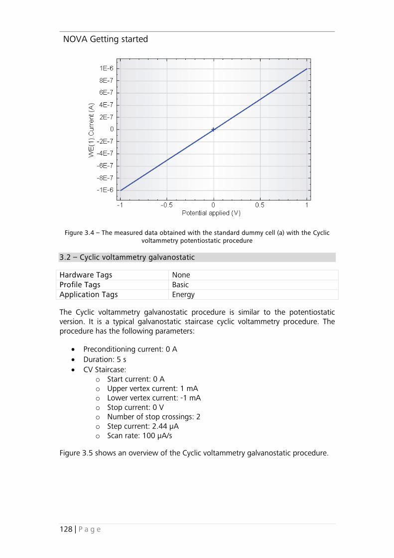
NOVA Getting started
128 | P a g e
Figure 3.4 – The measured data obtained with the standard dummy cell (a) with the Cyclic voltammetry potentiostatic procedure
3.2 – Cyclic voltammetry galvanostatic
Hardware Tags None Profile Tags Basic Application Tags Energy
The Cyclic voltammetry galvanostatic procedure is similar to the potentiostatic version. It is a typical galvanostatic staircase cyclic voltammetry procedure. The procedure has the following parameters:
• Preconditioning current: 0 A • Duration: 5 s • CV Staircase:
o Start current: 0 A o Upper vertex current: 1 mA o Lower vertex current: -1 mA o Stop current: 0 V o Number of stop crossings: 2 o Step current: 2.44 µA o Scan rate: 100 µA/s
Figure 3.5 shows an overview of the Cyclic voltammetry galvanostatic procedure.

NOVA Getting started
129 | P a g e
Figure 3.5 – The Cyclic voltammetry galvanostatic procedure
The signals sampled during this procedure are:
• Current applied • Time • Scan • WE(1).Potential • WE(1).Current • Index
Note
The automatic current ranging option is not available in galvanostatic mode (Please refer to Chapter 4 of this manual for more information on the Galvanostatic control restrictions.). This procedure uses the Autolab control command to set the instrument to galvanostatic mode and in the 1 mA current range before the measurement starts.

NOVA Getting started
130 | P a g e
Figure 3.6 shows a measurement on the dummy cell (c) with the Autolab Cyclic voltammetry galvanostatic procedure.
Figure 3.6 – The measured data obtained with the standard dummy cell (c) with the Cyclic voltammetry galvanostatic procedure
3.3 – Cyclic voltammetry current integration
Hardware Tags FI20 or on-board integrator Profile Tags Basic Application Tags Education, Energy, Interfacial electrochemistry
This procedure requires the optional FI20 module or the on-board integrator for the µAutolabII/III and the PGSTAT101. The procedure can be used to perform a cyclic voltammogram using the current integration method. This measurement technique uses a staircase potential profile but rather than sampling the current at the end of each step to minimize capacitive currents, the total current is accumulated in the analog integrator.
At the end of each step, the accumulated charge is reconverted in current. This integrated current includes both the Faradaic and the capacitive currents passed during the potential step. If the interval time is large (typically > 20 ms), the current response measured during a current integration cyclic voltammetry experiment can be compared, in first approximation, to the current measured with a true linear scan potential profile. More information about the use of the analog integrator is provided in the Filter and Integrator tutorial, available from the Help menu in NOVA.

NOVA Getting started
131 | P a g e
3.4 – Cyclic voltammetry linear scan
Hardware Tags SCAN250 or SCANGEN module Profile Tags Basic Application Tags Education, Energy, Interfacial electrochemistry
This procedure requires the optional SCAN250 or SCANGEN module. Both modules are linear scan generators. The procedure can be used to perform a cyclic voltammogram using a true linear scan potential profile rather than a staircase potential profile. More information about the use of these modules is provided in the Cyclic voltammetry linear scan tutorial, available from the Help menu in NOVA.
3.5 – Cyclic voltammetry linear scan high speed
Hardware Tags SCAN250 or SCANGEN in combination with ADC10M or ADC750 module
Profile Tags Basic Application Tags None
This procedure requires the optional SCAN250 or SCANGEN module and the optional ADC10M or ADC750 module. The SCAN250 and the SCANGEN are both linear scan generators. The ADC10M and the ADC750 are fast sampling analog to digital converters. The procedure can be used to perform a cyclic voltammogram using a true linear scan potential profile rather than a staircase potential profile, at high scan rate30. More information about the use of these modules is provided in the Cyclic voltammetry linear scan tutorial, available from the Help menu in NOVA.
30 Up to 10 kV/s with the SCANGEN+ADC750 or ADC10M and the SCAN250+ADC750; up to 250 kV/s with the SCAN250 + ADC10M.

NOVA Getting started
132 | P a g e
3.6 – Linear sweep voltammetry potentiostatic
Hardware Tags None Profile Tags Basic Application Tags Corrosion, Education, Electroanalysis, Energy,
Interfacial electrochemistry, Semiconductors
This procedure is a typical example of a staircase linear sweep voltammetry experiment in potentiostatic conditions. The procedure has the following parameters:
• Preconditioning potential: 0 V • Duration: 5 s • CV Staircase:
o Start potential: 0 V o Stop potential: 1 V o Step potential: 2.44 mV o Scan rate: 100 mV/s
Figure 3.7 shows an overview of the Linear sweep voltammetry potentiostatic procedure.
Figure 3.7 – The Linear sweep voltammetry potentiostatic procedure

NOVA Getting started
133 | P a g e
The signals sampled during this procedure are:
• Potential applied • Time • WE(1).Current • WE(1).Potential • Index
The procedure uses the Automatic current ranging option and displays the measured data as WE(1).Current vs Potential applied in the measurement view. Figure 3.8 shows a measurement on the dummy cell (a) with the Autolab Linear sweep voltammetry potentiostatic procedure.
Figure 3.8 – The measured data obtained with the standard dummy cell (a) with the Linear sweep voltammetry potentiostatic procedure

NOVA Getting started
134 | P a g e
3.7 – Linear sweep voltammetry galvanostatic
Hardware Tags None Profile Tags Basic Application Tags Energy
This procedure is a typical example of a staircase linear sweep voltammetry experiment in galvanostatic conditions. The procedure has the following parameters:
• Preconditioning current: 0 A • Duration: 5 s • CV Staircase:
o Start current: 0 A o Stop current: 1 mA o Step current: 2.44 µA o Scan rate: 100 µA/s
Figure 3.9 shows an overview of the Linear sweep voltammetry galvanostatic procedure.
Figure 3.9 – The Linear sweep voltammetry galvanostatic procedure

NOVA Getting started
135 | P a g e
The signals sampled during this procedure are:
• Current applied • Time • WE(1).Potential • WE(1).Current • Index
Figure 3.10 shows a measurement on the dummy cell (c) with the Autolab Linear sweep voltammetry galvanostatic procedure.
Figure 3.10 – The measured data obtained with the standard dummy cell (c) with the Linear sweep voltammetry galvanostatic procedure
Note
The automatic current ranging option is not available in galvanostatic mode (Please refer to Chapter 4 of this manual for more information on the Galvanostatic control restrictions.). This procedure uses the Autolab control command to set the instrument to galvanostatic mode and in the 1 mA current range before the measurement starts.

NOVA Getting started
136 | P a g e
3.8 – Linear polarization
Hardware Tags None Profile Tags Basic Application Tags Corrosion
The Linear polarization procedure measures the OCP potential (using the OCP determination command31) for the sample and then uses the Set reference potential command set the potential values of the linear sweep voltammetry relative to the averaged OCP (a moving average of 5 seconds is used).
The Linear polarization procedure has the following parameters:
• Measure OCP for 120 seconds with cutoff when dOCP/dt < 1 µV/s • Preconditioning potential: -100 mV (vs. OCP) • Duration: 5 s • LSV Staircase:
o Start potential: -100 mV (vs. OCP) o Stop potential: 100 mV (vs. OCP) o Step potential: 1 mV o Scan rate: 1 mV/s
Figure 3.11 shows an overview of the Linear polarization procedure.
31 Please refer to the Open circuit potential Tutorial, available from the Help menu, for more information on the OCP determination command.

NOVA Getting started
137 | P a g e
Figure 3.11 – The standard Linear polarization procedure
During the OCP determination, the following signals are sampled:
• Time • WE(1).Potential
The signals sampled during the linear sweep voltammetry measurement are:
• Potential applied • Time • WE(1).Current • WE(1).Potential • Index
At the end of the measurement, a corrosion rate calculation is performed.
Figure 3.12 shows a measurement on the dummy cell (c) with the Autolab Linear polarization procedure.

NOVA Getting started
138 | P a g e
Figure 3.12 – The measured data obtained with the standard dummy cell (a) with the Linear polarization procedure
3.9 – Hydrodynamic linear sweep
Hardware Tags Autolab RDE connected to DAC164 or Vout of Autolab
Profile Tags Basic Application Tags Corrosion, Education, Electroanalysis, Energy,
Interfacial electrochemistry
The Hydrodynamic linear sweep voltammetry procedure performs a linear sweep voltammetry using the Autolab RDE, with six different rotation rates. The rotation rate of the Autolab RDE is set using the Control Autolab RDE command linked to the values of a repeat for each value command32.
This procedure is intended to be used with the Remote switch of the Autolab motor controller enabled (on the back plane of the controller) and with a BNC cable connected between the DAC164 1 connector (Vout for the µAutolab II, III, the PGSTAT101, PGSTAT204 and the Multi Autolab) and the Remote input plug on the back plane of the Autolab RDE motor controller (see Figure 3.13).
32 Remote control of the Autolab RDE requires a BNC cable between the Autolab and the Autolab motor controller.

NOVA Getting started
139 | P a g e
Figure 3.13 – The Hydrodynamic linear sweep Voltammetry is intended to be used with the Autolab RDE and motor controller
Please refer to the Autolab RDE User Manual for more information.
The Hydrodynamic linear sweep voltammetry has the following parameters:
• Preconditioning potential: 1 V • Set RDE rotation rate to 0 RPM • Duration: 15 s • Repeat for each value
o Set RDE rotation rate o Wait 15 s o LSV Staircase
• Start potential: 1 V • Stop potential: 0 V • Step potential: -2.44 mV • Scan rate: 100 mV/s
Figure 3.14 shows an overview of the Hydrodynamic linear sweep voltammetry procedure.

NOVA Getting started
140 | P a g e
Figure 3.14 – The standard Hydrodynamic linear sweep procedure
The signals sampled during this procedure are:
• Potential applied • Time • WE(1).Current • WE(1).Potential • Index

NOVA Getting started
141 | P a g e
3.10 – Differential pulse voltammetry
Hardware Tags IME663 or IME303 interface Profile Tags Basic Application Tags Electroanalysis
This procedure, intended to be used in combination with a Mercury Drop Electrode (MDE) stand (Metrohm 663 VA, Princeton Applied Research 303/303A or other compatible MDE) provides an example of a differential pulse voltammetry measurement in NOVA.
This procedure requires the optional IME663 or IME303 module to be selected in the Hardware setup. More information about the use of these Autolab accessories is provided in the Voltammetric analysis tutorial, available from the Help menu in NOVA.
3.11 – Square wave voltammetry
Hardware Tags IME663 or IME303 interface Profile Tags Basic Application Tags Electroanalysis
This procedure, intended to be used in combination with a MDE stand (Metrohm 663 VA, Princeton Applied Research 303/303A or other compatible MDE) provides an example of a square wave voltammetry measurement in NOVA.
This procedure requires the optional IME663 or IME303 module to be selected in the Hardware setup. More information about the use of these Autolab accessories is provided in the Voltammetric analysis tutorial, available from the Help menu in NOVA.
3.12 – Sampled DC polarography
Hardware Tags IME663 or IME303 interface Profile Tags Basic Application Tags Electroanalysis
This procedure, intended to be used in combination with a MDE stand (Metrohm 663 VA, Princeton Applied Research 303/303A or other compatible MDE) provides
Note
The step value used in the Hydrodynamic linear sweep voltammetry procedure is negative because the sweep goes from 1 V to 0 V.

NOVA Getting started
142 | P a g e
an example of a sampled DC polarography measurement in NOVA. During this procedure, a new Hg drop is created at the end of each potential step.
This procedure requires the optional IME663 or IME303 module to be selected in the Hardware setup. More information about the use of these Autolab accessories is provided in the Voltammetric analysis tutorial, available from the Help menu in NOVA.
3.13 – Chrono amperometry (∆t > 1 ms)
Hardware Tags None Profile Tags Basic Application Tags Corrosion, Education, Electroanalysis, Energy,
Interfacial electrochemistry, Semiconductors
The Chrono amperometry (∆t > 1 ms) procedure has three consecutive potential steps. After each potential step, the current response is recorded during five seconds, with an interval time of 10 ms. The Record signals (>1 ms) command is used to measure the electrochemical signals. This command samples the signals with a smallest possible interval time of 1.30 ms.
The procedure has the following parameters:
• Preconditioning potential: 0 V • Duration: 5 s • Potential step 1: 0 V • Potential step 2: 0.5 V • Potential step 3: -0.5 V
Figure 3.15 shows an overview of the Chrono amperometry (∆t > 1 ms) procedure.
Figure 3.15 – The Chrono amperometry (∆t > 1 ms) procedure

NOVA Getting started
143 | P a g e
The signals sampled during this procedure are:
• Corrected time • WE(1).Potential • WE(1).Current • Time • Index
Figure 3.16 shows a measurement on the dummy cell (a) with the Autolab Chrono amperometry (∆t > 1 ms) procedure.
Figure 3.16 – The measured data obtained with the standard dummy cell (a) with the Chrono amperometry (∆t > 1 ms) procedure

NOVA Getting started
144 | P a g e
3.14 – Chrono potentiometry (∆t > 1 ms)
Hardware Tags None Profile Tags Basic Application Tags Corrosion, Energy, Interfacial electrochemistry
The Chrono potentiometry (∆t > 1 ms) procedure has three consecutive current steps. After each current step, the potential response is recorded during five seconds, with an interval time of 10 ms. The Record signals (>1 ms) command is used to measure the electrochemical signals. This command samples the signals with a smallest possible interval time of 1.30 ms.
The procedure has the following parameters:
• Preconditioning current: 0 A • Duration: 5 s • Potential step 1: 0 A • Potential step 2: 0.5 mA • Potential step 3: -0.5 mA
Figure 3.17 shows an overview of the Chrono potentiometry (∆t > 1 ms) procedure.
Figure 3.17 – The Chrono potentiometry (∆t > 1 ms) procedure
The signals sampled during this procedure are:
• Corrected time • WE(1).Potential • WE(1).Current • Time • Index

NOVA Getting started
145 | P a g e
Figure 3.18 shows a measurement on the dummy cell (c) with the Autolab Chrono potentiometry (∆t > 1 ms) procedure.
Figure 3.18 – The measured data obtained with the standard dummy cell (c) with the Chrono potentiometry (∆t > 1 ms) procedure
3.15 – Chrono amperometry fast
Hardware Tags None Profile Tags Basic Application Tags Interfacial electrochemistry
The Chrono amperometry fast procedure uses the Chrono methods command instead of the Record signals command. The Chrono methods command can be used for fast electrochemical measurements. The interval time can be lower than 1 ms33. Because this command works with higher sampling rates compared to the Record signals command, the data cannot be plotted real-time. The measured data is displayed at the end of the measurement.
The procedure has the following parameters:
• Preconditioning potential: 0 V • Duration: 5 s • Potential step 1: 0 V • Potential step 2: 0.3 V • Potential step 3: -0.3 V • Potential step 4: 0 V
33 Down to ~ 100 µs.

NOVA Getting started
146 | P a g e
The response of the cell is measured with an interval time of 100 µs. At the end of the measurement, switch to the analysis view to see the measured data points.
Figure 3.19 shows an overview of the Chrono amperometry fast procedure.
Figure 3.19 – The Chrono amperometry fast procedure
The levels used in this procedure are shown in Figure 3.20.

NOVA Getting started
147 | P a g e
Figure 3.20 – Overview of the levels used in the Chrono amperometry fast procedure
The signals sampled during this procedure are:
• Corrected time • Level • Time • WE(1).Current • Index
Figure 3.21 shows a measurement on the dummy cell (c) with the Autolab Chrono amperometry fast procedure.
Note
The automatic current ranging option is not available during the chrono methods measurement. This procedure uses the Autolab control command to set the instrument high speed and in the 1 mA current range before the measurement starts.

NOVA Getting started
148 | P a g e
Figure 3.21 – The measured data obtained with the standard dummy cell (c) with the Chrono amperometry fast procedure
Note
More information on time resolved measurements can be found in the Chrono methods tutorial, available from the Help menu in NOVA.
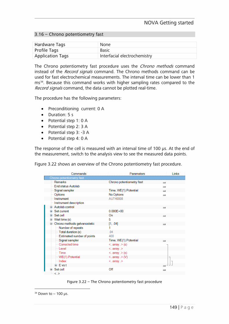
NOVA Getting started
149 | P a g e
3.16 – Chrono potentiometry fast
Hardware Tags None Profile Tags Basic Application Tags Interfacial electrochemistry
The Chrono potentiometry fast procedure uses the Chrono methods command instead of the Record signals command. The Chrono methods command can be used for fast electrochemical measurements. The interval time can be lower than 1 ms34. Because this command works with higher sampling rates compared to the Record signals command, the data cannot be plotted real-time.
The procedure has the following parameters:
• Preconditioning current: 0 A • Duration: 5 s • Potential step 1: 0 A • Potential step 2: 3 A • Potential step 3: -3 A • Potential step 4: 0 A
The response of the cell is measured with an interval time of 100 µs. At the end of the measurement, switch to the analysis view to see the measured data points.
Figure 3.22 shows an overview of the Chrono potentiometry fast procedure.
Figure 3.22 – The Chrono potentiometry fast procedure
34 Down to ~ 100 µs.
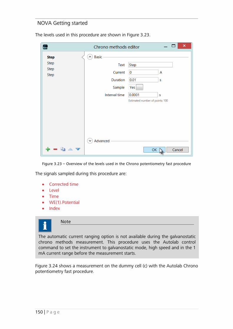
NOVA Getting started
150 | P a g e
The levels used in this procedure are shown in Figure 3.23.
Figure 3.23 – Overview of the levels used in the Chrono potentiometry fast procedure
The signals sampled during this procedure are:
• Corrected time • Level • Time • WE(1).Potential • Index
Figure 3.24 shows a measurement on the dummy cell (c) with the Autolab Chrono potentiometry fast procedure.
Note
The automatic current ranging option is not available during the galvanostatic chrono methods measurement. This procedure uses the Autolab control command to set the instrument to galvanostatic mode, high speed and in the 1 mA current range before the measurement starts.

NOVA Getting started
151 | P a g e
Figure 3.24 – The measured data obtained with the standard dummy cell (c) with the Chrono potentiometry fast procedure
3.17 – Chrono coulometry fast
Hardware Tags FI20 or on-board integrator Profile Tags Basic Application Tags Interfacial electrochemistry
This procedure requires the optional FI20 module or the on-board integrator for the µAutolabII/III, the PGSTAT101 and Multi Autolab with M101. The procedure can be used to perform chrono coulometric measurements. The integrator module provides a direct measurement of the charge. More information about the use of the analog integrator is provided in the Filter and Integrator tutorial, available from the Help menu in NOVA.
3.18 – Chrono amperometry high speed
Hardware Tags ADC10M or ADC750 module Profile Tags Basic Application Tags None
The Chrono amperometry high speed procedure uses the Chrono methods high speed command. This command requires the optional ADC10M or ADC750 module. Depending on the module, the shortest interval time is 100 ns (ADC10M) or 1.33 µs (ADC750).
More information about the use of these modules is provided in the Chrono methods high speed tutorial, available from the Help menu in NOVA.

NOVA Getting started
152 | P a g e
3.19 – Chrono potentiometry high speed
Hardware Tags ADC10M or ADC750 Profile Tags Basic Application Tags None
The Chrono potentiometry high speed procedure uses the Chrono methods high speed command. This command requires the optional ADC10M or ADC750 module. Depending on the module, the shortest interval time is 100 ns (ADC10M) or 1.33 µs (ADC750).
More information about the use of these modules is provided in the Chrono methods high speed tutorial, available from the Help menu in NOVA.
3.20 – Chrono charge discharge
Hardware Tags None Profile Tags Basic Application Tags Energy
The Chrono charge discharge procedure uses the Repeat n times command to repeat a combination of Set potential and Record signals (>1 ms) sequence. The response of the cell is recorded during 2.5 s, with an interval time of 10 ms. The Chrono charge discharge procedure has the following parameters:
• Preconditioning potential: 0 V • Duration: 5 s • Repeat 10 times
o Potential step 1: 1.2 V, duration: 2.5 s o Potential step 2: 0 V, duration: 2.5 s
Figure 3.25 shows an overview of the Chrono charge discharge procedure.

NOVA Getting started
153 | P a g e
Figure 3.25 – The Autolab Chrono charge discharge procedure
The signals sampled during this procedure are:
• Corrected time • Time • WE(1).Potential • WE(1).Current • Index
Figure 3.26 shows a measurement on the dummy cell (a) with the Autolab Chrono charge discharge procedure.

NOVA Getting started
154 | P a g e
Figure 3.26 – The measured data obtained with the standard dummy cell (a) with the Chrono charge discharge procedure
3.21 – i-Interrupt
Hardware Tags None Profile Tags Intermediate Application Tags None
This procedure can be used to perform a current interrupt measurement in order to determine the value of the uncompensated resistance.
More information about the use of this procedure is provided in the iR compensation tutorial, available from the Help menu in NOVA.
3.22 – i-Interrupt high speed
Hardware Tags ADC10M or ADC750 module Profile Tags Intermediate Application Tags None
This procedure is similar to the i-Interrupt procedure. This procedure uses the optional fast sampling ADC module (ADC750 or ADC10M).
Note
This procedure cannot be used in combination with the PGSTAT10 and the µAutolab type II/III.

NOVA Getting started
155 | P a g e
This procedure can be used to perform a current interrupt measurement in order to determine the value of the uncompensated resistance.
More information about the use of this procedure is provided in the iR compensation tutorial, available from the Help menu in NOVA.
3.23 – Positive feedback
Hardware Tags None Profile Tags Intermediate Application Tags None
The Positive feedback procedure provides the means to determine the value of the uncompensated resistance using the positive feedback method.
More information about the use of this procedure is provided in the iR compensation tutorial, available from the Help menu in NOVA.
3.24 – FRA impedance potentiostatic
Hardware Tags FRA32M or FRA2 module Profile Tags Basic Application Tags Corrosion, Energy, Interfacial electrochemistry,
Semiconductors
The FRA impedance potentiostatic procedure requires the optional FRA32M or FRA2 impedance analyzer module. This procedure can be used to perform a potentiostatic frequency scan to determine the electrochemical impedance of the cell.
More information about the use of the FRA32M or FRA2 module is provided in the Impedance tutorial, available from the Help menu in NOVA.
Note
This procedure cannot be used in combination with the PGSTAT10 and the µAutolab type II/III. This procedure requires the fast sampling ADC module.
Note
This procedure cannot be used in combination with the PGSTAT10 and the µAutolab type II/III.

NOVA Getting started
156 | P a g e
3.25 – FRA impedance galvanostatic
Hardware Tags FRA32M or FRA2 module Profile Tags Basic Application Tags Energy, Semiconductors
The FRA impedance galvanostatic procedure requires the optional FRA32M or FRA2 impedance analyzer module. This procedure can be used to perform a galvanostatic frequency scan to determine the electrochemical impedance of the cell.
More information about the use of the FRA32M or FRA2 module is provided in the Impedance tutorial, available from the Help menu in NOVA.
3.26 – FRA potential scan
Hardware Tags FRA32M or FRA2 module Profile Tags Intermediate Application Tags Semiconductors
The FRA potential scan procedure requires the optional FRA32M or FRA2 impedance analyzer module. This procedure can be used to perform a potentiostatic frequency scan at different DC potentials to determine the electrochemical impedance of the cell for each DC potential value.
More information about the use of the FRA32M or FRA2 module is provided in the Impedance tutorial, available from the Help menu in NOVA.

NOVA Getting started
157 | P a g e
The Autolab Potentiostat/Galvanostat
Nova can be used to control Autolab potentiostats/galvanostats with USB interface35. While the technical specifications of each of the instruments might be different, the operating principle remains the same.
This chapter provides an overview of the Autolab as well as information concerning the digital nature of the instrument. Information regarding noise issues is also provided.
4 – Autolab Hardware information 4.1 – Overview of the Autolab instrument
The Autolab instrument combined with the software is a computer-controlled electrochemical measurement system. It consists of a data-acquisition system and a potentiostat/galvanostat (see Figure 4.1).
Figure 4.1 – Overview of the Autolab potentiostat/galvanostat
The Autolab has the following key digital components:
• USB interface • Embedded real-time PC • Decoder and DIO controller
35 Except the PSTAT10 and the µAutolab type I.
re
Embedded real time PC
decoder
ce
wes
VF
CA
CF
ΣDAC164, FRA2SCAN250, EEXT
ADC164, FRA2ADC10M, FI20
Other modules
DIO
USB interface
Cell on/off
PSTAT/GSTAT

NOVA Getting started
158 | P a g e
The digital components are interfaced through the Autolab modules to the analog potentiostat/galvanostat circuit. The latter consists of the following components:
• The summation point (Σ) • The control amplifier (CA) • The voltage follower (VF) • The current follower (CF)
The summation point (Σ) is an adder circuit that feeds the input of the control amplifier. It is connected to the output of the several key modules of the Autolab:
• DAC164 • FRA36 DSG • SCAN25037 • Ein
Figure 4.2 shows a schematic overview of the different connections to the summation point of the Autolab potentiostat/galvanostat38. The labels shown in Figure 4.2 correspond to the dividing factors used for each signal on the summation point. For example, the signal generated by the FRA module (FRA-DSG) has a maximum amplitude of 3.5 V (RMS), which is divided by 10 at the input of the summation point, resulting in an effective maximum amplitude of 0.35 V (RMS).
Figure 4.2 – Mapping of the inputs of the summation point
36 This input is connected to the FRA32M or the FRA2 module. 37 Or earlier version SCANGEN. 38 Offset DAC, SCAN250/SCANGEN and Ein are not available on the µAutolab III. SCAN250/SCANGEN, FRA-DSG and Ein are not available on the PGSTAT101. SCAN250/SCANGEN and Ein are not available on the M101 module.
DAC164-1Offset DAC
± 10 V
ΣDAC164-2Scanning DAC
± 10 V
DAC164-4AC voltammetry DAC
± 10 V
FRA-DSG± 3.5 V (RMS)
Ein
± 10 V
SCAN250± 5 V
1÷10
1÷2
1÷2
1÷1
1÷1
1÷10

NOVA Getting started
159 | P a g e
The control amplifier provides the output voltage on the counter electrode (CE) with respect to the working electrode (WE) required to keep the potential difference between the reference electrode (RE) and the sense (S) at the user defined value, in potentiostatic mode, or the user required current between the counter electrode (CE) and the working electrode (WE) in galvanostatic mode.
The output of the control amplifier can be manually or remotely disconnected from the electrochemical cell through a cell ON/OFF switch. The voltage follower (VF) is used to measure the potential difference between the reference electrode and the sense and the current follower (CF). The current follower has several current ranges providing different current-to-voltage conversion factors.
The output of the CF and the VF are fed back to the analog-to-digital converter modules of the Autolab:
• ADC164 • FRA ADC39 • ADC10M40 • FI20
Furthermore, the output of the VF or the CF is fed back to the summation point to close the feedback loop in potentiostatic or galvanostatic mode, respectively.
The ADC164 provides the possibility of measuring analog signals. The input sensitivity is software-controlled, with ranges of ± 10 V (gain 1), ± 1 V (gain 10) and ± 0.1 V (gain 100). The resolution of the measurement is 1 in 65536 (16 bits, ADC164). Analog signals can be measured with a rate of up to 60 kHz. The ADC164 is used to measure the output of the Voltage Follower (VF) and Current Follower (CF) of the potentiostat/galvanostat module.
The DAC164 generates analog output signals. The output is software-controlled within a range of ± 10 V. The resolution of the DAC164 is 1 in 65535 (300 µV). In the Autolab PGSTAT two channels of the DAC are used to control the analog input signal of the potentiostat/galvanostat. The µAutolab only uses one DAC channel to control the analog input (see Figure 4.2). The values of the DACs are added up in the potentiostat and divided by 2. DAC channel 1 is used as a variable DAC and DAC channel 2 provides a fixed offset. This results in an output of ± 10 V with a resolution of 150 µV.
In practice this means that the potential range available with the Autolab PGSTAT during an electrochemical experiment is ± 5 V with respect to the offset potential generated by the offset DAC (DAC164-1). The available potential range is therefore -10 V to 10 V with the Autolab PGSTAT and -5 V to 5 V with the µAutolab.
39 These inputs are connected to the FRA32M or the FRA2 module. 40 Or earlier version ADC750.
NOVA Getting started
160 | P a g e
One additional DAC164 channel is available on the PGSTAT N series, DAC164-4. This channel is hardwired to the summation point and it is divided by 10. This input is used for measurements involving a small amplitude modulation (like AC voltammetry and AC voltammetry second harmonic). Presently, these methods and the use of this channel is not yet implemented in NOVA. The connection to the summation point can be removed if necessary41.
The DIO-part offers the possibility of controlling electrode systems, motorburettes or other equipment that can be controlled by TTL signals. This module can also be used to send or receive trigger signals to or from TTL devices. If an automatic mercury electrode such as PAR303 or Metrohm 663 VA Stand is used, gas purging and drop time can be activated. The interface for mercury electrodes, called IME303 or IME663, provides all necessary signals and connections for these electrodes, as well as for a drop knocker of a dropping mercury electrode (only for IME303).
The embedded PC can be in two different locations, depending on the type of interface:
• Inside of the Autolab-USB Interface box • Inside of the Autolab-USB instrument
41 Contact your Autolab distributor for more information.

NOVA Getting started
161 | P a g e
4.1.1 – Event timing in the Autolab
The embedded PC is equipped with a 1 MHz timer that is used by the software to control the timing of events during measurements. The shortest interval time on the embedded PC is 1 µs. When a procedure is started in NOVA, the procedure is first uploaded from the host PC to the embedded PC, through the USB connection. The measurement can then be started.
Depending on the type of command that NOVA encounters during the measurements two timing protocols are used:
1. Measurement commands: all measurement commands in NOVA are Timed commands. Whenever NOVA encounters a measurement command, it will be executed using the timing provided by the embedded computer of the Autolab. If several measurement commands are located in sequence, the sequence is executed without interruption. This ensures that the measurement commands in the sequence are executed with the smallest possible time gap. The actual time difference between two consecutive commands depends on the hardware changes required during the transition between the two commands. Switching current ranges or using the cell switch are time consuming steps since they involve mechanical relays which require a fixed settling time. Taking into account these hardware defined interval times, the effective time gap between two consecutive commands in a Timed procedure will be ≤ 10 ms.
2. Host commands: all the other commands in NOVA are host commands. These commands are executed by the host PC using the timing provided by this computer. Since the host PC is also involved in other Windows activity, accurate timing of events cannot be guaranteed and the effective interval time between two consecutive host commands will depend entirely on the amount of activity on the host PC. Depending on the command sequence, the time gap can be as short as ~ 2 s (transition between host command to measurement command) or several seconds (transition between measurement command and host command). Transfer of large amounts measured data points is particularly time consuming42.
42 The on-board memory of the fast sampling ADC module (ADC10M or ADC750) can store up to one million data points. Allow for gap times of several seconds when large data sets are transferred from the Autolab to the host computer.
Note
Measurement commands are identified by a green line on the left-hand side of the procedure editor.

NOVA Getting started
162 | P a g e
Figure 4.3 shows the Autolab Linear polarization procedure, in which measurement and host commands are identified using the green timing guide on left-hand side.
Figure 4.3 – The Autolab Linear polarization procedure (with the timing guide highlighted)
The procedure contains a series of measurement commands which are interrupted at two commands:
• OCP determination command • Corrosion rate, fit
These interruptions are indicated in the timing guide shown in Figure 4.3 by the matching breaks located right next to the two commands.
The OCP determination command is a host command because it requires the derivative of the measured OCP to be calculated during the measurement. The Corrosion rate, fit command is, like all analysis commands, a host command.
Timing guide

NOVA Getting started
163 | P a g e
The timing guide indicates that when this procedure is performed, a small interruption can be expected when the OCP determination command and when the Corrosion rate, fit command are executed.
4.2 – Consequence of the digital base of the Autolab
It is clear that the digital nature of the instrument has consequences for the measurements. The consequences for the different techniques are43:
• The minimum potential step or pulse in all techniques is 150 µV (16 Bit DAC164).
• All potential steps are rounded up or down to the nearest possible multiple of 150 µV.
• In cyclic voltammetry staircase, the interval time, Δ𝑡, or time between two consecutive steps is given by:
∆𝑡 =𝐸𝑠𝑡𝑒𝑝
Where 𝐸𝑠𝑡𝑒𝑝 is the potential step and is the scan rate in V/s.
The response of the electrochemical cell is recorded digitally. Therefore the resolution of the measurements is also limited. The actual resolution depends on the technique and on the amplitude of the signal. Since the A/D converter is equipped with a software programmable amplifier, the absolute resolution depends on the gain of the amplifier. The gains used are 1, 10 and 100 times the input signal.
NOVA automatically selects the best possible gain during a measurement. Gain 10 and 100 are used when the signal is small enough.
When the absolute value of the current is higher than (0.5 * current range), the resolution of the current measurement equals:
𝐶.𝑅.∙20216∙1
= 𝐶.𝑅.∙ 0.0003
When the absolute value of the current is lower than (0.5 * current range), the resolution equals:
43 The same applies for Galvanostatic control of the instrument.
Note
If needed, the Corrosion rate, fit command can be moved to the end of the procedure to prevent the interruption between the LSV staircase command and the Set cell command.

NOVA Getting started
164 | P a g e
𝐶.𝑅.∙ 20216 ∙ 10
= 𝐶.𝑅.∙ 0.00003
When the absolute value of the current is lower than (0.05 * current range), the resolution equals:
𝐶.𝑅.∙ 20216 ∙ 100
= 𝐶.𝑅.∙ 0.000003
The effect of the limited resolution can be seen, for instance when low currents are measured at a high current range. In such cases a lower current range has to be applied, if possible. When automatic current ranging is used, the most suitable current range is selected automatically.
Care must be taken when using this option in the following situations:
• High frequency square wave voltammetry is applied. • High scan rates in cyclic and linear sweep voltammetry are applied.
Switching of the current range takes about 0.5 ms to 2 ms. Therefore an erroneous point can be measured when the current range is switched. Most of the time, this error can be corrected by smoothing the plot afterwards.
4.3 – Autolab PGSTAT information
This section provides specific information for the Autolab PGSTAT series of instruments. The following instruments fall under this category: PGSTAT12, 128N, 30, 302, 302N, 100 and 100N44.
4.3.1 – Front panel and cell cable connection
There are four connectors on the front panel of the PGSTAT. The cable that connects to the WE and CE should be plugged into the WE/CE socket while the cable with the differential amplifier (leading to the RE, S and optionally WE2 electrodes) connects to the RE/S socket. A ground cable, embedded in the WE/CE cable connection, can be used to plug to the earth bulkhead for shielding purposes. Finally a monitor cable can be connected to a dedicated connector (see Figure 4.4).
44 For information on the PGSTAT302F, please refer to Section 4.4. For information on the PGSTAT101 and the Multi Autolab with M101 module, please refer to Section 4.5. For information on the µAutolab type II and III, please refer to Section 4.6.

NOVA Getting started
165 | P a g e
Figure 4.4 – Overview of the Autolab PGSTAT (top –Series 8 PGSTAT, bottom – Series 7 PGSTAT)
ADC164
WE/CE/Ground socket
Monitor cable inputDAC164
On/Off button Cell On/Off switchDigital display
RE/S socket
On/Off button Cell On/Off switchDigital display
ADC164
WE/CE socket
Monitor cable inputDAC164 RE/S socket
Ground connection
Note
The Series 7 instruments and early Series 8 instruments are provided with an additional ground cable which should be connected to the plug provided above the connector for the monitor cable. This ground connector should be used for grounding purposes.
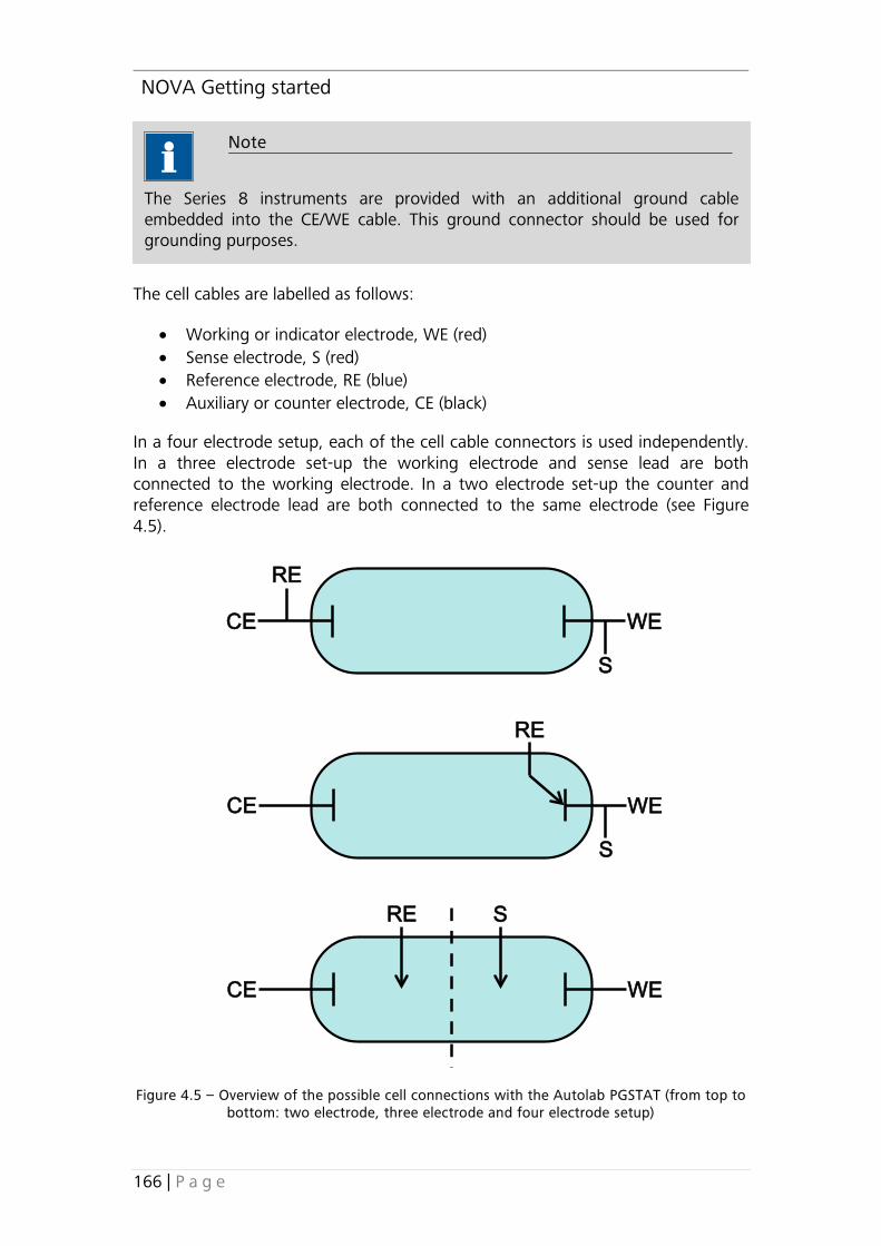
NOVA Getting started
166 | P a g e
The cell cables are labelled as follows:
• Working or indicator electrode, WE (red) • Sense electrode, S (red) • Reference electrode, RE (blue) • Auxiliary or counter electrode, CE (black)
In a four electrode setup, each of the cell cable connectors is used independently. In a three electrode set-up the working electrode and sense lead are both connected to the working electrode. In a two electrode set-up the counter and reference electrode lead are both connected to the same electrode (see Figure 4.5).
Figure 4.5 – Overview of the possible cell connections with the Autolab PGSTAT (from top to bottom: two electrode, three electrode and four electrode setup)
WECE
S
RE
WECE
S
RE
WECE
RE S
Note
The Series 8 instruments are provided with an additional ground cable embedded into the CE/WE cable. This ground connector should be used for grounding purposes.

NOVA Getting started
167 | P a g e
4.3.2 – Power up
The settings of the PGSTAT on power-up are pre-defined. The following settings are used:
• Cell: off • Mode: Potentiostatic • Bandwidth: High stability • iR Compensation: off • Current range: 10 mA • ECD mode: off, if applicable
4.3.3 – Connections for analog signals
The Autolab PGSTAT provides connections for analog signals through two different types of connectors:
• BNC connectors directly located on the front panel of the instrument • BNC connectors located on the monitor cable
4.3.3.1 – Connections for analog signals (front panel)
The ADC164 module and the DAC164 module are fitted with two analog inputs and two analog outputs, respectively (see Figure 4.6).
Figure 4.6 – Overview of the connections for analog signals provided on the front panel of the Autolab PGSTAT (ADC164 and DAC164)
ADC164 DAC164

NOVA Getting started
168 | P a g e
ADC164 – The ADC164 inputs, labelled 1 and 2 on the front panel, can be used to record any analog signal with a ± 10 V value range. The input impedance of the two analog inputs is 50 Ω.
DAC164 – The DAC164 outputs, labelled 1 and 2 on the front panel, can be used to generate any analog signal with a ± 10 V value range. The output impedance of these two inputs is 50 Ω. Corrections should be made with loads < 100 kΩ. Because of dissipation, the minimum load impedance should be 200 Ω.
4.3.3.2 – Connections for analog signals (monitor cable)
With the supplied monitor cable, there are a number of BNC connectors to the PGSTAT analog circuits (see Figure 4.7). All the signals are with respect to Autolab ground and indirectly to protective earth. Avoid creating ground loops as this will often degrade the performance of the PGSTAT.
Note
The DAC164 1 and 2 outputs are identified as DAC channels 3 and 4, respectively in the Set DAC command.

NOVA Getting started
169 | P a g e
Figure 4.7 – The monitor cable for the Series 8 and the Series 7 PGSTAT
The following signals are available:
EOUT – This output corresponds to the differential potential of RE versus S45. The output voltage will vary between ±10 V. The output impedance is 50 Ω, so a correction should be made if a load < 100 kΩ is connected. The minimum load impedance is 200 Ω.
iOUT – This signal corresponds to the output of the current-to-voltage converter circuit of the PGSTAT. A 1 V signal corresponds to 1 x the selected current range. The output level varies between ± 10 V. The output impedance is 50 Ω, so a correction should be made if a load < 100 kΩ is connected. The minimum load impedance is 200 Ω.
EIN – This is an analog voltage input, that can only be used after it has been enabled in software, using the Autolab control command (see Figure 4.8). Do not leave it enabled unnecessarily, to prevent noise pickup by the system. This input is directly connected to the summation point, Σ, of the PGSTAT. In PSTAT mode, a
45 The Eout value corresponds to -WE(1).Potential.

NOVA Getting started
170 | P a g e
1 V signal will add 1 V to the cell voltage, while in GSTAT mode a 1 V signal adds an extra current of 1 x the selected current range to flow. In both cases, the external signal adds to any pre-defined voltage or current. The input voltage range is ± 10 V. Input impedance is 1 kΩ (only when input is activated) so a correction should be made when the source impedance is > 1 Ω.
Figure 4.8 – The external input is enabled in the Autolab control window
4.3.4 – High stability, High speed and Ultra high speed
The PGSTAT is equipped with three different bandwidth settings: High stability (HSTAB), High speed and Ultra high speed. The bandwidth can be defined using the Autolab control command (see Figure 4.9).

NOVA Getting started
171 | P a g e
Figure 4.9 – The Autolab control window can be used to set the bandwidth of the PGSTAT
The purpose of these different modes of operation is to provide a maximum bandwidth, maintaining stability in the PSTAT or GSTAT control loop. The normal mode of operation is High stability46. This gives the Control Amplifier a bandwidth of 12.5 kHz. The HSTAB indicator on the front panel of the PGSTAT and in the Autolab display is lit when the High stability mode is active (see Figure 4.10).
Figure 4.10 – A HSTAB indicator is provided on the Autolab display
46 Power up default setting.

NOVA Getting started
172 | P a g e
This setting is the most appropriate for measurements at low frequencies or low scan rates. The noise in the i and E signals will be minimized. Measurements at high frequency or at high scan rates require a faster mode of operation.
When operating in High speed mode, the control amplifier will have its bandwidth extended with one decade up to 125 kHz. Some cells can show ringing or oscillation using this setting, particularly highly capacitive cells in PSTAT mode. Increasing the bandwidth also increases the noise levels for the i and E signals. The High speed mode is automatically selected during impedance measurement at frequencies > 10 kHz.
For applications requiring very high bandwidth, the Ultra high speed mode can be selected. In this mode, the control amplifier bandwidth is extended to 500 kHz (PGSTAT12, PGSTAT128N, PGSTAT100 and PGSTAT100N) or 1.25 MHz (PGSTAT30, PGSTAT302 and PGSTAT302N). There is a significant oscillation risk using this setting, and the noise levels will generally show an increase relative to the High speed or High stability mode. The Ultra high speed mode is automatically selected during impedance measurements at frequencies > 100 kHz, while the High stability mode is selected for frequencies below 10 kHz (see Figure 4.11).
Figure 4.11 – Bandwidth limits in the Autolab PGSTAT
4.3.5 – RE input impedance and stability
The electrometer RE input contains a small capacitive load. If the capacitive part of the impedance between CE and RE is comparatively large, phase shifts will occur which can lead to instability problems when working in potentiostatic mode. If the
High speed High stability Ultra high speed
10 kHz 100 kHz
Note
It is possible to switch from High stability to High speed by clicking the HSTAB label in the Autolab display. In High speed mode, this label will be unlit, both on the front panel of the PGSTAT and on the Autolab display. Clicking the HSTAB label again switches the bandwidth back to High stability.
Warning
The higher the bandwidth, the more important it is to pay attention to adequate shielding of the cell and the electrode connectors. The use of a Faraday cage is recommended in this case.

NOVA Getting started
173 | P a g e
impedance between the CE and the RE cannot be changed and oscillations are observed, it is recommended to select the High stability mode to increase the system stability. In general, the use of High stability leads to a more stable control loop, compared to High speed or Ultra high speed and a significantly lower bandwidth.
To make use of the full potentiostat bandwidth (Ultra high speed mode), the impedance between CE and RE has to be lower than 35 kΩ47. This value is derived by testing. In galvanostat mode, this large impedance between CE and RE, will usually not lead to stability problems, because of the current feedback regulation.
4.3.6 – Galvanostatic FRA measurements
The capacitive part of the impedance between RE and ground is an important aspect to consider when performing FRA measurements in galvanostat mode. Large reference electrode impedance values may introduce a phase shift at low frequencies. The origin of the phase shift between the CE and the RE cannot be determined from the FRA data.
Galvanostatic FRA measurements at 1 MHz require a maximum of 3 kΩ reference electrode impedance to keep phase errors within the ± 5 º limit.
4.3.7 – Galvanostat, potentiostat and iR-compensation bandwidth
For galvanostatic measurements on low current ranges, the bandwidth limiting factor becomes the current-to-voltage circuit rather than the control amplifier.
For stability reasons it is not recommended to use the High speed mode for current ranges < 10 μA. The Ultra high speed mode is also not recommended for current ranges < 1 mA.
As the current measurement circuit plays an important role in the iR compensation technique, its use is also subject to bandwidth limitations.
47 Empirical value.

NOVA Getting started
174 | P a g e
A general indication of the maximum available bandwidth for GSTAT and for iR compensation can be found in Table 4.1:
Instrument PGSTAT12/128N/100/100N PGSTAT30/302/302N Mode GSTAT iR/C – PSTAT GSTAT iR/C – PSTAT 1 A – 1 mA > 500 kHz > 500 kHz > 1.25 MHz > 1.25 MHz 100 µA 125 kHz 500 kHz 125 kHz 1 MHz 10 µA 100 kHz 100 kHz 100 kHz 100 kHz 1 µA 10 kHz 10 kHz 10 kHz 10 kHz 100 nA 1 kHz 1 kHz 1 kHz 1 kHz 10 nA 100 Hz 100 Hz 100 Hz 100 Hz
Table 4.1 – Bandwidth overview for the different instruments
At the same time, the iR-compensation bandwidth limits indicate up to which frequency current measurements can be made in potentiostatic mode (either with or without iR compensation).
4.3.8 – Galvanostatic operation and current range linearity
For galvanostatic experiments, automatic current ranging is not possible. The measurements are performed in a fixed current range. Each current range on the instrument is characterized by a specific linearity limit and this specification determines the maximum current that can be applied in galvanostatic mode.
The linearity limitation also applies on measurements performed in potentiostatic mode in a fixed current range.
Table 4.2 provides an overview of the current range linearity for the different PGSTAT instruments.

NOVA Getting started
175 | P a g e
Current range PGSTAT12 PGSTAT100 PGSTAT100N
PGSTAT128N PGSTAT30 PGSTAT302 PGSTAT302N
1 A n.a. 0.8 1 2 100 mA 2.5 3 3 3 10 – 1 mA 3 3 3 3 100 – 1 µA 3 3 3 3 100 – 10 nA 3 3 3 3
Table 4.2 – Linearity limit for the different instruments
For example, in the 100 mA current range, the maximum current that can be applied, galvanostatically, using the PGSTAT302N, is 300 mA. The maximum current that can be measured in the 100 mA current range, using the same instrument is 1000 mA, although currents exceeding 300 mA will be measured outside of the linearity limit of this current range.
In galvanostatic operation, the applied current values are checked during the procedure validation step. When the applied current exceeds the linearity limit for the specified current range, an error message will be shown in the procedure validation screen (see Figure 4.12).
Figure 4.12 – The procedure validation step always checks the applied current values for the allowed linearity

NOVA Getting started
176 | P a g e
Figure 4.13 – When a current overload is detected, a suggestion is shown in the user log
4.3.9 – Oscillation detection
The PGSTAT has a detector for large-amplitude oscillation. The detector will spot any signal swing that causes the control amplifier to produce both a positive and a negative Voltage overload within ~ 200 μs. Thus, large oscillations at frequencies > 2.5 kHz will be detected. Upon oscillation, the OSC indicator on the PGSTAT front panel will be activated. The Vovl warning will also be shown in the Autolab display. An oscillation protection feature can be enabled or disabled in the software, using the Autolab control command (see Figure 4.14).
Figure 4.14 – The Autolab control window can be used to switch the oscillation protection on or off
Note
In potentiostatic mode, this check is not performed. It is possible to measure a current value in a fixed current range, even if the current value exceeds the linearity limit of the active current range. This triggers a current overload warning. When this happens during a measurement, a message will be shown in the user log, suggesting a modification of the current range (see Figure 4.13).

NOVA Getting started
177 | P a g e
If the oscillation protection is enabled, the occurrence of oscillation will also immediately turn off the manual cell switch of the Autolab. When this happens, both the OSC indicator and the manual cell switch start blinking. The Autolab display will show the message ‘Cell manually off’ (see Figure 4.15).
Figure 4.15 – The cell manually off is displayed when the oscillation protection circuit is triggered
The cell may be switched on again by pressing the manual cell switch button. If oscillation resumes, the cell switch will be turned off as soon as the button is released. Holding the button pressed in, provides an opportunity to observe the system during oscillation.
Some cells that cause ringing when switching the cell on or changing the current range can falsely trigger the oscillation detector. If this happens, the Oscillation protection may be switched off in the software in order to prevent an accidental disconnection of the cell.
4.3.10 – Maximum reference electrode voltage
The differential electrometer input contains an input protection circuitry that becomes active after crossing the ±10 V limit. This is implemented to avoid electrometer damage. Please note that the Vovl indicator will not light up for this type of voltage overload. The measured voltage will be cutoff at an absolute value of 10.00 V.
Depending on the cell properties, galvanostatic control of the cell could lead to a potential difference between the RE and the S/WE larger than 10 V. This situation will trigger the cutoff of the measured voltage to prevent overloading the differential amplifier.

NOVA Getting started
178 | P a g e
4.3.11 – Active cells
Some electrochemical cells such as batteries and fuel cells are capable of delivering power to the PGSTAT. This is allowed only to a maximum ‘cell’ power, PMAX. This value depends on the instrument (see Table 4.3).
Instrument Maximum power, PMAX (W) PGSTAT12 2.5 PGSTAT128N 8 PGSTAT30 10 PGSTAT302/302N 20 PGSTAT100/100N 2.5
Table 4.3 – Maximum power rating for the different PGSTAT models
This means that cells showing an absolute voltage (|Vcell|) of less than 10 V between WE and CE are intrinsically safe. They may drive the PGSTAT output stage into current limit but will not overload the amplifier. On the other hand, cells that have an absolute voltage higher than 10 V between WE and CE may only deliver a maximum current, iMAX given by:
𝑖𝑀𝐴𝑋 =𝑃𝑀𝐴𝑋
|𝑉𝑀𝐴𝑋|
4.3.12 – Grounded cells
The measurement circuitry of the Autolab is internally connected to protective earth (P.E.). This can be an obstacle when measurement is desired of a cell that is itself in contact with P.E. In such a case, undefined currents will flow through the loop that is formed when the electrode connections from the PGSTAT are linked to the cell and measurements will not be possible. Please note that not only a short circuit or a resistance can make a connection to earth, but also a capacitance is capable of providing a conductive path (for AC signals). The earth connection between the cell and P.E. should always be broken. If there is no possibility of doing this, please contact Metrohm Autolab for a custom solution, if available.
4.3.13 – Environmental conditions
The PGSTAT may be used at temperatures of 0 to 40 degrees Celsius. The instrument is calibrated at 25 degrees Celsius and will show minimum errors at that temperature. The ventilation holes on the bottom plate and on the rear panel may never be obstructed, nor should the instrument be placed in direct sunlight or near other sources of heat.
4.3.14 – Temperature overload
As a safety precaution, the PGSTAT is equipped with a circuit that monitors the temperature of the internal power electronics. A temperature overload will be displayed as a blinking indicator in the manual cell switch, with the cell

NOVA Getting started
179 | P a g e
automatically turned off. You will not be able to turn the cell back on until the temperature inside the instrument has fallen to an acceptable level. It can then be switched on again by pressing the manual cell switch button on the front panel.
During normal operation the temperature should never become extremely high and no temperature overload will occur. If this does happen, the origin of the temperature overload should be identified:
1. Is the room temperature unusually high? 2. Was the PGSTAT oscillating? 3. Is the voltage selector for mains power set to the right value? 4. Is the fan turning and are all the ventilation holes unobstructed? 5. Was the cell delivering a considerable amount of power to the PGSTAT? 6. Are the WE and CE cables shorted in PSTAT mode48?
If a temperature overload takes place repeatedly, for no obvious reason, Metrohm Autolab recommends having the instrument checked by their service department.
4.3.15 – Noise
When measuring low level currents, some precautions should be taken in order to minimize noise. The personal computer must be placed as far away as possible from the electrochemical cell and the cell cables. The cell cables should not cross other electrical cables. Other equipment with power supplies can also cause noise. For instance, the interface for mercury electrodes IME should also be placed with some care. If possible place the computer between the PGSTAT and other equipments. Avoid using unshielded extension cables to the electrodes. The use of a Faraday cage is also advised.
If the cell system has a ground connector, it can be connected to the analog ground connector at the front of the PGSTAT. If a Faraday cage is used, it should be connected to this ground connector. Some experiments concerning optimization of the signal-to-noise ratio can readily indicate whether or not a configuration is satisfactory.
More information on noise is provided in section 4.8.
48 This must never occur!

NOVA Getting started
180 | P a g e
4.4 – Autolab PGSTAT302F information
This section provides specific information for the Autolab PGSTAT302F. The PGSTAT302F is a special version of the Autolab PGSTAT302N which can be operated in so-called floating mode49. In floating mode, the PGSTAT302F can be used to control the potential of grounded working electrodes. In this configuration, the Autolab is floating with respect to the working electrode sample. Additionally, the PGSTAT302F can be operated in non-floating mode in combination with working electrode disconnected from ground.
49 The compliance voltage of the PGSTAT302F is +/- 10 V in floating mode. The compliance voltage in grounded mode is +/- 10 V with the default cell cables and +/- 30 V with optional modified cell cables. Please contact your Autolab distributor for more information.
Warning
The floating mode of the special PGSTAT302N must only be used on grounded working electrodes. The working electrode can be grounded using the green ground connector embedded in the CE/WE cable of the PGSTAT302F.
Warning
Instrument performance can be substantially degraded when the PGSTAT302F is operated in floating mode. The instrument specifications provided by Metrohm Autolab can only be achieved when the PGSTAT302F is used in non-floating mode.
Note
Special precautions must be taken with the cell connections when the PGSTAT302F is used in floating mode. Only the working electrode can be connected to ground, all other electrodes must be isolated from ground. External equipments connected to the PGSTAT302F must be isolated when the instrument is used in floating mode. Keep in mind that grounding of external equipment can occur through connections to a computer, if applicable (for example through a USB or RS232 cable).

NOVA Getting started
181 | P a g e
4.4.1 – Front panel and cell cable connection
There are four connectors on the front panel of the PGSTAT. The cable that connects to the WE and CE should be plugged into the WE/CE socket while the cable with the differential amplifier (leading to the RE, S and optionally WE2 electrodes) connects to the RE/S socket. A ground cable, embedded in the WE/CE cable connection, can be used to plug to the earth bulkhead for shielding purposes. Finally a monitor cable can be connected to a dedicated connector (see Figure 4.16).
Figure 4.16 – Overview of the Autolab PGSTAT302F
The cell cables are labelled as follows:
• Working or indicator electrode, WE (red) • Sense electrode, S (red) • Reference electrode, RE (blue) • Auxiliary or counter electrode, CE (black)
In a four electrode setup, each of the cell cable connectors is used independently. In a three electrode set-up the working electrode and sense lead are both connected to the working electrode. In a two electrode set-up the counter and reference electrode lead are both connected to the same electrode (see Figure 4.17).
ADC164
WE/CE/Ground socket
Monitor cable inputDAC164
On/Off button Cell On/Off switchDigital display
RE/S socket

NOVA Getting started
182 | P a g e
Figure 4.17 – Overview of the possible cell connections with the Autolab PGSTAT302F (from top to bottom: two electrode, three electrode and four electrode setup)
4.4.2 – Power up
The settings of the PGSTAT on power-up are pre-defined. The following settings are used:
• Cell: off • Mode: Potentiostatic • Bandwidth: High stability • iR Compensation: off • Current range: 10 mA
WECE
S
RE
WECE
S
RE
WECE
RE S
Warning
In floating mode, the iOVL warning may be lit when the cell is off. This warning can be ignored.

NOVA Getting started
183 | P a g e
4.4.3 – Connections for analog signals
The Autolab PGSTAT302F provides connections for analog signals through two different types of connectors:
• BNC connectors directly located on the front panel of the instrument • BNC connectors located on the monitor cable
4.4.3.1 – Connections for analog signals (front panel)
The ADC164 module and the DAC164 module are fitted with two analog inputs and two analog outputs, respectively (see Figure 4.18).
Figure 4.18 – Overview of the connections for analog signals provided on the front panel of the Autolab PGSTAT (ADC164 and DAC164)
ADC164 – The ADC164 inputs, labelled 1 and 2 on the front panel, can be used to record any analog signal with a ± 10 V value range. The input impedance of the two analog inputs is 50 Ω.
DAC164 – The DAC164 outputs, labelled 1 and 2 on the front panel, can be used to generate any analog signal with a ± 10 V value range. The output impedance of these two inputs is 50 Ω. Corrections should be made with loads < 100 kΩ. Because of dissipation, the minimum load impedance should be 200 Ω.
These inputs are floating when the PGSTAT302F is operated in floating mode. Connected equipment may not be connected to ground and the shield of the BNC cables may not be connected to safety ground.
ADC164 DAC164
Note
The DAC164 1 and 2 outputs are identified as DAC channels 3 and 4, respectively in the Set DAC command.

NOVA Getting started
184 | P a g e
Avoid creating ground loops as this will often degrade the performance of the PGSTAT302F.
4.4.3.2 – Connections for analog signals (monitor cable)
With the supplied monitor cable, there are a number of BNC connectors to the PGSTAT analog circuits (see Figure 4.19). All the signals are with respect to Autolab ground and indirectly to protective earth when the PGSTAT302F is operated in normal mode.
These signals are floating when the PGSTAT302F is operated in floating mode. Connected equipment may not be connected to ground and the shield of the BNC cables may not be connected to safety ground.
Avoid creating ground loops as this will often degrade the performance of the PGSTAT302F.
Figure 4.19 – The monitor cable for the PGSTAT302F
The following signals are available:
EOUT – This output corresponds to the differential potential of S versus RE50. The output voltage will vary between ±10 V. The output impedance is 50 Ω, so a correction should be made if a load < 100 kΩ is connected. The minimum load impedance is 200 Ω.
iOUT – This signal corresponds to the output of the current-to-voltage converter circuit of the PGSTAT51. A 1 V signal corresponds to -1 x the selected current range. The output level varies between ± 10 V. The output impedance is 50 Ω, so a correction should be made if a load < 100 kΩ is connected. The minimum load impedance is 200 Ω.
EIN – This is an analog voltage input, that can only be used after it has been enabled in software, using the Autolab control command (see Figure 4.20). Do not leave it enabled unnecessarily, to prevent noise pickup by the system. This input is directly connected to the summation point, Σ, of the PGSTAT. In PSTAT mode, a
50 The Eout value corresponds to WE(1).Potential. 51 The iout value corresponds to -WE(1).Current.

NOVA Getting started
185 | P a g e
1 V signal will add -1 V to the cell voltage, while in GSTAT mode a 1 V signal adds an extra current of -1 x the selected current range to flow. In both cases, the external signal adds to any pre-defined voltage or current. The input voltage range is ± 10 V. Input impedance is 1 kΩ (only when input is activated) so a correction should be made when the source impedance is > 1 Ω.
Figure 4.20 – The external input is enabled in the Autolab control window
4.4.4 – High stability and High speed
The PGSTAT302F is equipped with two different bandwidth settings: High stability (HSTAB) and High speed. The bandwidth can be defined using the Autolab control command (see Figure 4.21).

NOVA Getting started
186 | P a g e
Figure 4.21 – The Autolab control window can be used to set the bandwidth of the PGSTAT
The purpose of these different modes of operation is to provide a maximum bandwidth, maintaining stability in the PSTAT or GSTAT control loop. The normal mode of operation is High stability52. This gives the Control Amplifier a bandwidth of 12.5 kHz. The HSTAB indicator on the front panel of the PGSTAT and in the Autolab display is lit when the High stability mode is active (see Figure 4.22).
Figure 4.22 – A HSTAB indicator is provided on the Autolab display
52 Power up default setting.

NOVA Getting started
187 | P a g e
This setting is the most appropriate for measurements at low frequencies or low scan rates. The noise in the i and E signals will be minimized. Measurements at high frequency or at high scan rates require a faster mode of operation.
When operating in High speed mode, the control amplifier will have its bandwidth extended with one decade up to 125 kHz. Some cells can show ringing or oscillation using this setting, particularly highly capacitive cells in PSTAT mode. Increasing the bandwidth also increases the noise levels for the i and E signals. The High speed mode is automatically selected during impedance measurement at frequencies > 10 kHz.
The High speed mode is automatically selected during impedance measurements at frequencies > 10 kHz, while the High stability mode is selected for frequencies below 10 kHz (see Figure 4.23).
Figure 4.23 – Bandwidth limits in the Autolab PGSTAT302F
4.4.5 – RE input impedance and stability
The electrometer RE input contains a small capacitive load. If the capacitive part of the impedance between CE and RE is comparatively large, phase shifts will occur which can lead to instability problems when working in potentiostatic mode. If the impedance between the CE and the RE cannot be changed and oscillations are observed, it is recommended to select the High stability mode to increase the system stability. In general, the use of High stability leads to a more stable control loop, compared to High speed or Ultra high speed and a significantly lower bandwidth.
High stability High speed
10 kHz
Note
It is possible to switch from High stability to High speed by clicking the HSTAB label in the Autolab display. In High speed mode, this label will be unlit, both on the front panel of the PGSTAT and on the Autolab display. Clicking the HSTAB label again switches the bandwidth back to High stability.
Warning
The higher the bandwidth, the more important it is to pay attention to adequate shielding of the cell and the electrode connectors. The use of a Faraday cage is recommended in this case.

NOVA Getting started
188 | P a g e
To make use of the full potentiostat bandwidth (High speed mode), the impedance between CE and RE has to be lower than 35 kΩ53. This value is derived by testing. In galvanostat mode, this large impedance between CE and RE, will usually not lead to stability problems, because of the current feedback regulation.
4.4.6 – Galvanostatic FRA measurements
The capacitive part of the impedance between RE and ground is an important aspect to consider when performing FRA measurements in galvanostat mode. Large reference electrode impedance values may introduce a phase shift at low frequencies. The origin of the phase shift between the CE and the RE cannot be determined from the FRA data.
Galvanostatic FRA measurements at 1 MHz require a maximum of 3 kΩ reference electrode impedance to keep phase errors within the ± 5 º limit.
4.4.7 – Galvanostat, potentiostat and iR-compensation bandwidth
For galvanostatic measurements on low current ranges, the bandwidth limiting factor becomes the current-to-voltage circuit rather than the control amplifier.
For stability reasons it is not recommended to use the High speed mode for current ranges < 10 μA.
As the current measurement circuit plays an important role in the iR compensation technique, its use is also subject to bandwidth limitations. A general indication of the maximum available bandwidth for GSTAT and for iR compensation can be found in Table 4.4:
Mode GSTAT iR/C - PSTAT 1 A – 1 mA > 500 kHz > 500 kHz 100 µA 125 kHz 500 kHz 10 µA 100 kHz 100 kHz 1 µA 10 kHz 10 kHz 100 nA 1 kHz 1 kHz 10 nA 100 Hz 100 Hz
Table 4.4 – Bandwidth overview for the PGSTAT302F
At the same time, the iR-compensation bandwidth limits indicate up to which frequency current measurements can be made in potentiostatic mode (either with or without iR compensation).
53 Empirical value.

NOVA Getting started
189 | P a g e
4.4.8 – Galvanostatic operation and current range linearity
For galvanostatic experiments, automatic current ranging is not possible. The measurements are performed in a fixed current range. Each current range on the instrument is characterized by a specific linearity limit and this specification determines the maximum current that can be applied in galvanostatic mode.
The linearity limitation also applies on measurements performed in potentiostatic mode in a fixed current range.
Table 4.5 provides an overview of the current range linearity for the PGSTAT302F.
Current range Linearity 1 A 2 100 mA 3 10 – 1 mA 3 100 – 1 µA 3 100 – 10 nA 3
Table 4.5 – Linearity limit for the PGSTAT302F
For example, in the 100 mA current range, the maximum current that can be applied, galvanostatically, using the PGSTAT302F, is 300 mA. The maximum current that can be measured in the 100 mA current range, using the same instrument is 1000 mA, although currents exceeding 300 mA will be measured outside of the linearity limit of this current range.
In galvanostatic operation, the applied current values are checked during the procedure validation step. When the applied current exceeds the linearity limit for the specified current range, an error message will be shown in the procedure validation screen (see Figure 4.24).
Figure 4.24 – The procedure validation step always checks the applied current values for the allowed linearity

NOVA Getting started
190 | P a g e
Figure 4.25 – When a current overload is detected, a suggestion is shown in the user log
4.4.9 – Oscillation detection
The PGSTAT302F has a detector for large-amplitude oscillation. The detector will spot any signal swing that causes the control amplifier to produce both a positive and a negative Voltage overload within ~ 200 μs. Thus, large oscillations at frequencies > 2.5 kHz will be detected. Upon oscillation, the OSC indicator on the PGSTAT front panel will be activated. The Vovl warning will also be shown in the Autolab display. An oscillation protection feature can be enabled or disabled in the software, using the Autolab control command (see Figure 4.26).
Note
In potentiostatic mode, this check is not performed. It is possible to measure a current value in a fixed current range, even if the current value exceeds the linearity limit of the active current range. This triggers a current overload warning. When this happens during a measurement, a message will be shown in the user log, suggesting a modification of the current range (see Figure 4.25).

NOVA Getting started
191 | P a g e
Figure 4.26 – The Autolab control window can be used to switch the oscillation protection on or off
If the oscillation protection is enabled, the occurrence of oscillation will also immediately turn off the manual cell switch of the Autolab. When this happens, both the OSC indicator and the manual cell switch start blinking. The Autolab display will show the message ‘Cell manually off’ (see Figure 4.27).
Figure 4.27 – The cell manually off is displayed when the oscillation protection circuit is triggered

NOVA Getting started
192 | P a g e
The cell may be switched on again by pressing the manual cell switch button. If oscillation resumes, the cell switch will be turned off as soon as the button is released. Holding the button pressed in, provides an opportunity to observe the system during oscillation.
Some cells that cause ringing when switching the cell on or changing the current range can falsely trigger the oscillation detector. If this happens, the Oscillation protection may be switched off in the software in order to prevent an accidental disconnection of the cell.
4.4.10 – Maximum reference electrode voltage
The differential electrometer input contains an input protection circuitry that becomes active after crossing the ±10 V limit. This is implemented to avoid electrometer damage. Please note that the Vovl indicator will not light up for this type of voltage overload. The measured voltage will be cutoff at an absolute value of 10.00 V.
Depending on the cell properties, galvanostatic control of the cell could lead to a potential difference between the RE and the S/WE larger than 10 V. This situation will trigger the cutoff of the measured voltage to prevent overloading the differential amplifier.
4.4.11 – Active cells
Some electrochemical cells such as batteries and fuel cells are capable of delivering power to the PGSTAT302F. This is allowed only to a maximum ‘cell’ power, PMAX of 20 W.
This means that cells showing an absolute voltage (|Vcell|) of less than 10 V between WE and CE are intrinsically safe. They may drive the PGSTAT output stage into current limit but will not overload the amplifier. On the other hand, cells that have an absolute voltage higher than 10 V between WE and CE may only deliver a maximum current, iMAX given by:
𝑖𝑀𝐴𝑋 =𝑃𝑀𝐴𝑋
|𝑉𝑀𝐴𝑋|

NOVA Getting started
193 | P a g e
4.4.12 – Grounded cells and grounded working electrodes
The PGSTAT302F can be operated in two different modes:
• Normal mode: this mode corresponds to the operating mode using in all the PGSTAT instruments. For more information on the restrictions applying to this mode, please refer to section 4.3.12.
• Floating mode: this mode is only available on the PGSTAT302F. In this mode, measurement circuitry of the Autolab is internally disconnected to protective earth (P.E.). This allows the instrument to be used in combination with a grounded working electrode or a grounded cell.
The PGSTAT302F can be set to either normal mode or floating mode using a dedicated short-circuit plug on the back plane of the instrument (see Figure 4.28). When the short-circuit plug is connected as shown in Figure 4.28, the instrument operates in normal mode. When the short-circuit plug is disconnected from the back panel, the instrument operates in floating mode.
Figure 4.28 – The PGSTAT302F can be set to normal mode (left) or to floating mode (right) using the provided short-circuit plug

NOVA Getting started
194 | P a g e
4.4.13 – Environmental conditions
The PGSTAT302F may be used at temperatures of 0 to 40 degrees Celsius. The instrument is calibrated at 25 degrees Celsius and will show minimum errors at that temperature. The ventilation holes on the bottom plate and on the rear panel may never be obstructed, nor should the instrument be placed in direct sunlight or near other sources of heat.
4.4.14 – Temperature overload
As a safety precaution, the PGSTAT302F is equipped with a circuit that monitors the temperature of the internal power electronics. A temperature overload will be displayed as a blinking indicator in the manual cell switch, with the cell automatically turned off. You will not be able to turn the cell back on until the temperature inside the instrument has fallen to an acceptable level. It can then be switched on again by pressing the manual cell switch button on the front panel.
During normal operation the temperature should never become extremely high and no temperature overload will occur. If this does happen, the origin of the temperature overload should be identified:
1. Is the room temperature unusually high? 2. Was the PGSTAT oscillating? 3. Is the voltage selector for mains power set to the right value? 4. Is the fan turning and are all the ventilation holes unobstructed? 5. Was the cell delivering a considerable amount of power to the PGSTAT? 6. Are the WE and CE cables shorted in PSTAT mode54?
If a temperature overload takes place repeatedly, for no obvious reason, Metrohm Autolab recommends having the instrument checked by their service department.
4.4.15 – Noise
When measuring low level currents, some precautions should be taken in order to minimize noise. The personal computer must be placed as far away as possible from the electrochemical cell and the cell cables. The cell cables should not cross other electrical cables. Other equipment with power supplies can also cause noise. For instance, the interface for mercury electrodes IME should also be placed with some care. If possible place the computer between the PGSTAT302F and other equipments. Avoid using unshielded extension cables to the electrodes. The use of a Faraday cage is also advised.
54 This must never occur!

NOVA Getting started
195 | P a g e
If the cell system has a ground connector, it can be connected to the analog ground connector at the front of the PGSTAT302F. If a Faraday cage is used, it should be connected to this ground connector. Some experiments concerning optimization of the signal-to-noise ratio can readily indicate whether or not a configuration is satisfactory.
More information on noise is provided in Section 4.8.
4.5 – Autolab PGSTAT101 and M101 information
This section provides specific information for the Autolab PGSTAT101 and the M101 potentiostat/galvanostat module for the Multi Autolab.
4.5.1 – Front panel and cell cable connection (PGSTAT101)
There are two connectors on the front panel of the PGSTAT101. The cell cable should be plugged into the CELL socket on the front panel of the instrument. The I/O socket on the front panel can be used to connect the optional I/O cable (see Figure 4.29).
Figure 4.29 – Overview of the Autolab PGSTAT101 (front)
POTENTIOSTATGALVANOSTAT
PGSTAT101
I / O
CELL
Status LED
I/O cable socket
Cell cable socket
Warning
Instrument performance can be substantially degraded when the PGSTAT302F is operated in floating mode. The instrument specifications provided by Metrohm Autolab can only be achieved when the PGSTAT302F is used in non-floating mode.

NOVA Getting started
196 | P a g e
The cell cable is labelled as follows:
• Working or indicator electrode, WE (red) • Sense electrode, S (red) • Reference electrode, RE (blue) • Auxiliary or counter electrode, CE (black)
An additional ground connection (for shielding purposes, e.g. a Faraday cage) is also provided with the cell cable.
In a four electrode setup, each of the cell cable connectors is used independently. In a three electrode set-up the working electrode and sense lead are both connected to the working electrode. In a two electrode set-up the counter and reference electrode lead are both connected to the same electrode (see Figure 4.30).
Figure 4.30 – Overview of the possible cell connections with the Autolab PGSTAT101 (from top to bottom: two electrode, three electrode and four electrode setup)
4.5.2 – Front panel and cell cable connection (M101)
The M101 potentiostat/galvanostat module can be installed in the Multi Autolab frame, up to a maximum of 12 modules in a single frame. The M101 is identical in
WECE
S
RE
WECE
S
RE
WECE
RE S

NOVA Getting started
197 | P a g e
specification to the PGSTAT101. All information provided in the rest of section 4.5 applies to both the PGSTAT101 and the M10155 installed in the Multi Autolab.
There are three connectors on the front panel of each M101 module installed in the Multi Autolab (see Figure 4.31).
Figure 4.31 – Overview of the M101 (front) in Multi Autolab frame
Each M101 module is identified by a module label on the front panel, indicating the location and the purpose of each connector (see Figure 4.32)
Figure 4.32 – Detailed view of the M101 module label
55 In the rest of this section, the M101 and PGSTAT101 will be referred to as PGSTAT101.
Status LED
I/O cable socket
Cell cable socket
DIO cable socket
Cell status LED

NOVA Getting started
198 | P a g e
The cell cable should be plugged into the lowest socket, labelled by the symbol , on the front panel of the module. The I/O socket on the front panel can be used to connect the optional I/O cable. The DIO cable, used to connect to the optional IME663 or IME303 or for TTL triggering, can be connected to the DIO connector on the front panel.
The cell cable is labelled as follows:
• Working or indicator electrode, WE (red) • Sense electrode, S (red) • Reference electrode, RE (blue) • Auxiliary or counter electrode, CE (black)
An additional ground connection (for shielding purposes, e.g. a Faraday cage) is also provided with the cell cable.
In a four electrode setup, each of the cell cable connectors is used independently. In a three electrode set-up the working electrode and sense lead are both connected to the working electrode. In a two electrode set-up the counter and reference electrode lead are both connected to the same electrode (see Figure 4.30).
4.5.3 – Power up
The settings of the PGSTAT101 on power-up are pre-defined. The following settings are used:
• Cell: off • Mode: Potentiostatic • Bandwidth: High stability • iR Compensation: off • Current range: 1 µA
4.5.4 – Connections for analog signals
With the optional I/O cable, four additional connections are provided to the PGSTAT101 analog circuits (see Figure 4.33). All the signals are with respect to Autolab ground and indirectly to protective earth. Avoid creating ground loops as this will often degrade the performance of the PGSTAT.
Note
Specific information on Multi Autolab can be found in the Multi Autolab tutorial, available from the Help menu.

NOVA Getting started
199 | P a g e
Figure 4.33 – The optional I/O cable for the PGSTAT101 (top) and M101 (bottom)
The following signals are available:
EOUT – This output corresponds to the differential potential of RE versus S56. The output voltage will vary between ±10 V. The output impedance is 1 kΩ, so a correction should be made if a load < 2 MΩ is connected. The maximum bandwidth is 300 kHz.
iOUT – This signal corresponds to the inverted output of the current-to-voltage converter circuit of the PGSTAT10157. A 1 V signal corresponds to -1 x the selected current range. The output level varies between ± 10 V. The output impedance is 50 Ω, so a correction should be made if a load < 100 kΩ is connected. The minimum load impedance is 200 Ω.
VOUT – This output corresponds to the DAC output. It is controlled by software and is meant to be used to control external devices, like the rotating speed of a
56 The Eout value corresponds to -WE(1).Potential. 57 The iout value corresponds to -WE(1).Current/Current range.

NOVA Getting started
200 | P a g e
Rotating Disc Electrode (RDE). The output level varies between ±10 V and the output impedance is very low, < 1 Ω. The output amplifier is capable of providing 5 mA at full scale, so load impedance should be > 2 kΩ.
VIN – This input corresponds to the ADC input. This input can be used for measuring a second signal. The input range is ±10 V and the input impedance is 50 Ω.
4.5.5 – High stability, High speed and Ultra high speed
The PGSTAT101 is equipped with three different bandwidth settings: High stability (HSTAB), High speed and Ultra high speed. The bandwidth can be defined using the Autolab control command (see Figure 4.34).
Figure 4.34 – The Autolab control window can be used to set the bandwidth of the PGSTAT101
The purpose of these different modes of operation is to provide a maximum bandwidth, maintaining stability in the PSTAT or GSTAT control loop. The normal mode of operation is High stability58. This gives the Control Amplifier a bandwidth of 12.5 kHz. The HSTAB indicator in the Autolab display is lit when the High stability mode is active (see Figure 4.35).
58 Power up default setting.

NOVA Getting started
201 | P a g e
Figure 4.35 – A HSTAB indicator is provided on the Autolab display
This setting is the most appropriate for measurements at low frequencies or low scan rates. The noise in the i and E signals will be minimized. Measurements at high frequency or at high scan rates require a faster mode of operation.
When operating in High speed mode, the control amplifier will have its bandwidth extended with one decade up to 125 kHz. Some cells can show ringing or oscillation using this setting, particularly highly capacitive cells in PSTAT mode. Increasing the bandwidth also increases the noise levels for the i and E signals.
For applications requiring very high bandwidth, the Ultra high speed mode can be selected. In this mode, the control amplifier bandwidth is extended to 1 MHz. There is a significant oscillation risk using this setting, and the noise levels will generally show an increase relative to the High speed or High stability mode.
Note
It is possible to switch from High stability to High speed by clicking the HSTAB label in the Autolab display. In High speed mode, this label will be unlit on the Autolab display. Clicking the HSTAB label again switches the bandwidth back to High stability.
Warning
The higher the bandwidth, the more important it is to pay attention to adequate shielding of the cell and the electrode connectors. The use of a Faraday cage is recommended in this case.

NOVA Getting started
202 | P a g e
4.5.6 – RE input impedance and stability
The electrometer RE input contains a small capacitive load. If the capacitive part of the impedance between CE and RE is comparatively large, phase shifts will occur which can lead to instability problems when working in potentiostatic mode. If the impedance between the CE and the RE cannot be changed and oscillations are observed, it is recommended to select the High stability mode to increase the system stability. In general, the use of High stability leads to a more stable control loop, compared to High speed or Ultra high speed and a significantly lower bandwidth.
To make use of the full potentiostat bandwidth (Ultra high speed mode), the impedance between CE and RE has to be lower than 35 kΩ59. This value is derived by testing. In galvanostat mode, this large impedance between CE and RE, will usually not lead to stability problems, because of the current feedback regulation.
4.5.7 – Galvanostat, potentiostat and iR-compensation bandwidth
For galvanostatic measurements on low current ranges, the bandwidth limiting factor becomes the current-to-voltage circuit rather than the control amplifier.
For stability reasons it is not recommended to use the High speed mode for current ranges < 10 μA. The Ultra high speed mode is also not recommended for current ranges < 1 mA.
As the current measurement circuit plays an important role in the iR compensation technique, its use is also subject to bandwidth limitations. A general indication of the maximum available bandwidth for GSTAT and for iR compensation can be found in Table 4.6:
Mode GSTAT iR/C - PSTAT 10 mA – 1 mA > 1 MHz > 1 MHz 100 µA 1 MHz 1 MHz 10 µA 10 kHz 75 kHz 1 µA 10 kHz 20 kHz 100 nA 400 Hz 4 kHz 10 nA 400 Hz 400 Hz
Table 4.6 – Bandwidth overview for the PGSTAT101
At the same time, the iR-compensation bandwidth limits indicate up to which frequency current measurements can be made in potentiostatic mode (either with or without iR compensation).
59 Empirical value.

NOVA Getting started
203 | P a g e
4.5.8 – Galvanostatic operation and current range linearity
For galvanostatic experiments, automatic current ranging is not possible. The measurements are performed in a fixed current range. Each current range on the instrument is characterized by a specific linearity limit and this specification determines the maximum current that can be applied in galvanostatic mode.
The linearity limitation also applies on measurements performed in potentiostatic mode in a fixed current range.
Table 4.7 provides an overview of the current range linearity for the PGSTAT101.
Current range Linearity 10 mA 10 1 mA 7 10 – 1 mA 7 100 – 1 µA 7 100 – 10 nA 7
Table 4.7 – Linearity limit for the PGSTAT101
For example, in the 1 mA current range, the maximum current that can be applied, galvanostatically, using the PGSTAT101, is 7 mA. The maximum current that can be measured in the 1 mA current range is 10 mA, although currents exceeding 7 mA will be measured outside of the linearity limit of this current range.
In galvanostatic operation, the applied current values are checked during the procedure validation step. When the applied current exceeds the linearity limit for the specified current range, an error message will be shown in the procedure validation screen (see Figure 4.36).
Figure 4.36 – The procedure validation step always checks the applied current values for the allowed linearity
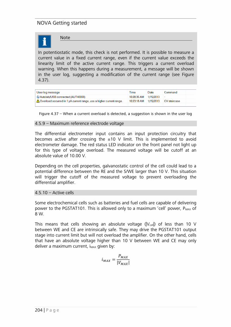
NOVA Getting started
204 | P a g e
Figure 4.37 – When a current overload is detected, a suggestion is shown in the user log
4.5.9 – Maximum reference electrode voltage
The differential electrometer input contains an input protection circuitry that becomes active after crossing the ±10 V limit. This is implemented to avoid electrometer damage. The red status LED indicator on the front panel not light up for this type of voltage overload. The measured voltage will be cutoff at an absolute value of 10.00 V.
Depending on the cell properties, galvanostatic control of the cell could lead to a potential difference between the RE and the S/WE larger than 10 V. This situation will trigger the cutoff of the measured voltage to prevent overloading the differential amplifier.
4.5.10 – Active cells
Some electrochemical cells such as batteries and fuel cells are capable of delivering power to the PGSTAT101. This is allowed only to a maximum ‘cell’ power, PMAX of 8 W.
This means that cells showing an absolute voltage (|Vcell|) of less than 10 V between WE and CE are intrinsically safe. They may drive the PGSTAT101 output stage into current limit but will not overload the amplifier. On the other hand, cells that have an absolute voltage higher than 10 V between WE and CE may only deliver a maximum current, iMAX given by:
𝑖𝑀𝐴𝑋 =𝑃𝑀𝐴𝑋
|𝑉𝑀𝐴𝑋|
Note
In potentiostatic mode, this check is not performed. It is possible to measure a current value in a fixed current range, even if the current value exceeds the linearity limit of the active current range. This triggers a current overload warning. When this happens during a measurement, a message will be shown in the user log, suggesting a modification of the current range (see Figure 4.37).

NOVA Getting started
205 | P a g e
4.5.11 – Grounded cells
The measurement circuitry of the Autolab is internally connected to protective earth (P.E.). This can be an obstacle when measurement is desired of a cell that is itself in contact with P.E. In such a case, undefined currents will flow through the loop that is formed when the electrode connections from the PGSTAT101 are linked to the cell and measurements will not be possible. Please note that not only a short circuit or a resistance can make a connection to earth, but also a capacitance is capable of providing a conductive path (for AC signals). The earth connection between the cell and P.E. should always be broken. If there is no possibility of doing this, please contact Metrohm Autolab for a custom solution, if available.
4.5.12 – Environmental conditions
The PGSTAT101 may be used at temperatures of 0 to 40 degrees Celsius. The instrument is calibrated at 25 degrees Celsius and will show minimum errors at that temperature. The ventilation holes on the bottom plate and on the rear panel may never be obstructed, nor should the instrument be placed in direct sunlight or near other sources of heat.
4.5.13 – Noise
When measuring low level currents, some precautions should be taken in order to minimize noise. The personal computer must be placed as far away as possible from the electrochemical cell and the cell cables. The cell cables should not cross other electrical cables. Other equipment with power supplies can also cause noise. For instance, the interface for mercury electrodes IME should also be placed with some care. If possible place the computer between the PGSTAT101 and other equipments. Avoid using unshielded extension cables to the electrodes. The use of a Faraday cage is also advised.
If the cell system has a ground connector, it can be connected to the analog ground connector provided with the cell cable of the PGSTAT101. If a Faraday cage is used, it should be connected to this ground connector. Some experiments concerning optimization of the signal-to-noise ratio can readily indicate whether or not a configuration is satisfactory.
More information on noise is provided in section 4.8.

NOVA Getting started
206 | P a g e
4.6 – Autolab PGSTAT204 information
This section provides specific information for the Autolab PGSTAT204.
4.6.1 – Front panel and cell cable connections
The PGSTAT204 potentiostat/galvanostat module is installed into the Autolab PGSTAT204 instrument, alongside one optional module. From the front view, the PGSTAT204 module is always installed in the leftmost module bay. There are three connectors on the front panel of the PGSTAT204 module (see Figure 4.38).
Figure 4.38 – Overview of the PGSTAT204 module (front)
The cell cable should be plugged into the lowest socket, labelled by the symbol , on the front panel of the PGSTAT204 module. The I/O socket on the front panel can be used to connect the optional I/O cable. The DIO cable, used to connect to the optional IME663 or IME303 or for TTL triggering, can be connected to the DIO connector on the front panel.
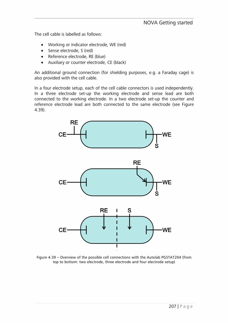
NOVA Getting started
207 | P a g e
The cell cable is labelled as follows:
• Working or indicator electrode, WE (red) • Sense electrode, S (red) • Reference electrode, RE (blue) • Auxiliary or counter electrode, CE (black)
An additional ground connection (for shielding purposes, e.g. a Faraday cage) is also provided with the cell cable.
In a four electrode setup, each of the cell cable connectors is used independently. In a three electrode set-up the working electrode and sense lead are both connected to the working electrode. In a two electrode set-up the counter and reference electrode lead are both connected to the same electrode (see Figure 4.39).
Figure 4.39 – Overview of the possible cell connections with the Autolab PGSTAT204 (from top to bottom: two electrode, three electrode and four electrode setup)
WECE
S
RE
WECE
S
RE
WECE
RE S

NOVA Getting started
208 | P a g e
4.6.2 – Power up
The settings of the PGSTAT204 on power-up are pre-defined. The following settings are used:
• Cell: off • Mode: Potentiostatic • Bandwidth: High stability • iR Compensation: off • Current range: 1 µA
4.6.3 – Connections for analog signals
With the optional I/O cable, four additional connections are provided to the PGSTAT204 analog circuits (see Figure 4.40). All the signals are with respect to Autolab ground and indirectly to protective earth. Avoid creating ground loops as this will often degrade the performance of the PGSTAT.
Figure 4.40 – The optional I/O cable for the PGSTAT204
The following signals are available:
EOUT – This output corresponds to the differential potential of RE versus S60. The output voltage will vary between ±10 V. The output impedance is 1 kΩ, so a correction should be made if a load < 2 MΩ is connected. The maximum bandwidth is 300 kHz.
iOUT – This signal corresponds to the inverted output of the current-to-voltage converter circuit of the PGSTAT20461. A 1 V signal corresponds to -1 x the selected current range. The output level varies between ± 10 V. The output
60 The Eout value corresponds to -WE(1).Potential. 61 The iout value corresponds to -WE(1).Current/Current range.

NOVA Getting started
209 | P a g e
impedance is 50 Ω, so a correction should be made if a load < 100 kΩ is connected. The minimum load impedance is 200 Ω.
VOUT – This output corresponds to the DAC output. It is controlled by software and is meant to be used to control external devices, like the rotating speed of a Rotating Disc Electrode (RDE). The output level varies between ±10 V and the output impedance is very low, < 1 Ω. The output amplifier is capable of providing 5 mA at full scale, so load impedance should be > 2 kΩ.
VIN – This input corresponds to the ADC input. This input can be used for measuring a second signal. The input range is ±10 V and the input impedance is 50 Ω.
4.6.4 – High stability, High speed and Ultra high speed
The PGSTAT204 is equipped with three different bandwidth settings: High stability (HSTAB), High speed and Ultra high speed. The bandwidth can be defined using the Autolab control command (see Figure 4.41).
Figure 4.41 – The Autolab control window can be used to set the bandwidth of the PGSTAT204
The purpose of these different modes of operation is to provide a maximum bandwidth, maintaining stability in the PSTAT or GSTAT control loop. The normal mode of operation is High stability62. This gives the Control Amplifier a bandwidth of 12.5 kHz. The HSTAB indicator in the Autolab display is lit when the High stability mode is active (see Figure 4.42). 62 Power up default setting.

NOVA Getting started
210 | P a g e
Figure 4.42 – A HSTAB indicator is provided on the Autolab display
This setting is the most appropriate for measurements at low frequencies or low scan rates. The noise in the i and E signals will be minimized. Measurements at high frequency or at high scan rates require a faster mode of operation.
When operating in High speed mode, the control amplifier will have its bandwidth extended with one decade up to 125 kHz. Some cells can show ringing or oscillation using this setting, particularly highly capacitive cells in PSTAT mode. Increasing the bandwidth also increases the noise levels for the i and E signals.
For applications requiring very high bandwidth, the Ultra high speed mode can be selected. In this mode, the control amplifier bandwidth is extended to 1 MHz. There is a significant oscillation risk using this setting, and the noise levels will generally show an increase relative to the High speed or High stability mode.
Note
It is possible to switch from High stability to High speed by clicking the HSTAB label in the Autolab display. In High speed mode, this label will be unlit on the Autolab display. Clicking the HSTAB label again switches the bandwidth back to High stability.
Warning
The higher the bandwidth, the more important it is to pay attention to adequate shielding of the cell and the electrode connectors. The use of a Faraday cage is recommended in this case.

NOVA Getting started
211 | P a g e
4.6.5 – RE input impedance and stability
The electrometer RE input contains a small capacitive load. If the capacitive part of the impedance between CE and RE is comparatively large, phase shifts will occur which can lead to instability problems when working in potentiostatic mode. If the impedance between the CE and the RE cannot be changed and oscillations are observed, it is recommended to select the High stability mode to increase the system stability. In general, the use of High stability leads to a more stable control loop, compared to High speed or Ultra high speed and a significantly lower bandwidth.
To make use of the full potentiostat bandwidth (Ultra high speed mode), the impedance between CE and RE has to be lower than 35 kΩ63. This value is derived by testing. In galvanostat mode, this large impedance between CE and RE, will usually not lead to stability problems, because of the current feedback regulation.
4.6.6 – Galvanostat, potentiostat and iR-compensation bandwidth
For galvanostatic measurements on low current ranges, the bandwidth limiting factor becomes the current-to-voltage circuit rather than the control amplifier.
For stability reasons it is not recommended to use the High speed mode for current ranges < 10 μA. The Ultra high speed mode is also not recommended for current ranges < 1 mA.
As the current measurement circuit plays an important role in the iR compensation technique, its use is also subject to bandwidth limitations. A general indication of the maximum available bandwidth for GSTAT and for iR compensation can be found in Table 4.8:
Mode GSTAT iR/C - PSTAT 100 mA – 100 µA > 1 MHz > 1 MHz 10 µA 10 kHz 50 kHz 1 µA 10 kHz 50 kHz 100 nA 500 Hz 500 Hz 10 nA 500 Hz 500 Hz
Table 4.8 – Bandwidth overview for the PGSTAT204
At the same time, the iR-compensation bandwidth limits indicate up to which frequency current measurements can be made in potentiostatic mode (either with or without iR compensation).
4.6.7 – Galvanostatic operation and current range linearity
For galvanostatic experiments, automatic current ranging is not possible. The measurements are performed in a fixed current range. Each current range on the
63 Empirical value.

NOVA Getting started
212 | P a g e
instrument is characterized by a specific linearity limit and this specification determines the maximum current that can be applied in galvanostatic mode.
The linearity limitation also applies on measurements performed in potentiostatic mode in a fixed current range.
Table 4.9 provides an overview of the current range linearity for the PGSTAT204.
Current range Linearity 100 mA 4 10 mA 7 1 mA 7 10 – 1 mA 7 100 – 1 µA 7 100 – 10 nA 7
Table 4.9 – Linearity limit for the PGSTAT204
For example, in the 1 mA current range, the maximum current that can be applied, galvanostatically, using the PGSTAT204, is 7 mA. The maximum current that can be measured in the 1 mA current range is 10 mA, although currents exceeding 7 mA will be measured outside of the linearity limit of this current range.
In galvanostatic operation, the applied current values are checked during the procedure validation step. When the applied current exceeds the linearity limit for the specified current range, an error message will be shown in the procedure validation screen (see Figure 4.43).

NOVA Getting started
213 | P a g e
Figure 4.43 – The procedure validation step always checks the applied current values for the allowed linearity
Figure 4.44 – When a current overload is detected, a suggestion is shown in the user log
Note
In potentiostatic mode, this check is not performed. It is possible to measure a current value in a fixed current range, even if the current value exceeds the linearity limit of the active current range. This triggers a current overload warning. When this happens during a measurement, a message will be shown in the user log, suggesting a modification of the current range (see Figure 4.44).

NOVA Getting started
214 | P a g e
4.6.8 – Maximum reference electrode voltage
The differential electrometer input contains an input protection circuitry that becomes active after crossing the ±10 V limit. This is implemented to avoid electrometer damage. The red status LED indicator on the front panel will not light up for this type of voltage overload. The measured voltage will be cutoff at an absolute value of 10.00 V.
Depending on the cell properties, galvanostatic control of the cell could lead to a potential difference between the RE and the S/WE larger than 10 V. This situation will trigger the cutoff of the measured voltage to prevent overloading the differential amplifier.
4.6.9 – Active cells
Some electrochemical cells such as batteries and fuel cells are capable of delivering power to the PGSTAT204. This is allowed only to a maximum ‘cell’ power, PMAX of 8 W.
This means that cells showing an absolute voltage (|Vcell|) of less than 10 V between WE and CE are intrinsically safe. They may drive the PGSTAT204 output stage into current limit but will not overload the amplifier. On the other hand, cells that have an absolute voltage higher than 10 V between WE and CE may only deliver a maximum current, iMAX given by:
𝑖𝑀𝐴𝑋 =𝑃𝑀𝐴𝑋
|𝑉𝑀𝐴𝑋|
4.6.10 – Grounded cells
The measurement circuitry of the Autolab is internally connected to protective earth (P.E.). This can be an obstacle when measurement is desired of a cell that is itself in contact with P.E. In such a case, undefined currents will flow through the loop that is formed when the electrode connections from the PGSTAT204 are linked to the cell and measurements will not be possible. Please note that not only a short circuit or a resistance can make a connection to earth, but also a capacitance is capable of providing a conductive path (for AC signals). The earth connection between the cell and P.E. should always be broken. If there is no possibility of doing this, please contact Metrohm Autolab for a custom solution, if available.
4.6.11 – Environmental conditions
The PGSTAT204 may be used at temperatures of 0 to 40 degrees Celsius. The instrument is calibrated at 25 degrees Celsius and will show minimum errors at that temperature. The ventilation holes on the bottom plate and on the rear panel may never be obstructed, nor should the instrument be placed in direct sunlight or near other sources of heat.

NOVA Getting started
215 | P a g e
4.6.12 – Noise
When measuring low level currents, some precautions should be taken in order to minimize noise. The personal computer must be placed as far away as possible from the electrochemical cell and the cell cables. The cell cables should not cross other electrical cables. Other equipment with power supplies can also cause noise. For instance, the interface for mercury electrodes IME should also be placed with some care. If possible place the computer between the PGSTAT204 and other equipments. Avoid using unshielded extension cables to the electrodes. The use of a Faraday cage is also advised.
If the cell system has a ground connector, it can be connected to the analog ground connector provided with the cell cable of the PGSTAT204. If a Faraday cage is used, it should be connected to this ground connector. Some experiments concerning optimization of the signal-to-noise ratio can readily indicate whether or not a configuration is satisfactory.
More information on noise is provided in Section 4.8.
4.6.13 – Temperature overload
The PGSTAT204 is fitted with a temperature overload protection circuit. When the instrument reaches the maximum operating temperature, the protection circuit will trigger and the cell will be disconnected. The instrument will then enter in predefined safe mode and it will no longer be possible to switch the cell on. To reset the instrument, the device must be switched off, allowed to cool and then switched on again.
When the temperature overload circuit is triggered, the status LED on the front panel of the PGSTAT204 will be lit red and the corresponding indicator in the Autolab display will also be lit (see Figure 4.45).
Figure 4.45 – The T ovl indicator is let when the temperature overload circuit is triggered

NOVA Getting started
216 | P a g e
4.7 – µAutolab information
This section provides specific information for the µAutolab64.
4.7.1 – Front panel and cell cable connection
There is a single connector on the front panel of the µAutolab, used to connect the cell cables (see Figure 4.46).
Figure 4.46 – Overview of the µAutolab
The cell cables are labelled as follows:
• Working or indicator electrode, WE (red) • Reference electrode, RE (blue) • Auxiliary or counter electrode, CE (black)
In a two electrode set-up the counter and reference electrode lead are both connected to the same electrode (see Figure 4.47).
64 The µAutolab type I is not supported in NOVA.
On/Off switch Cell On/Off switch
Display Cell cable socket

NOVA Getting started
217 | P a g e
Figure 4.47 – Overview of the possible cell connections with the µAutolab (two electrode, top and three electrode setup, bottom)
4.7.2 – Power up
The settings of the µAutolab on power-up are pre-defined. The following settings are used:
• Cell: off • Mode: Potentiostatic • Bandwidth: High stability • Current range: 1 µA
4.7.3 – Connections for analog signals
On the rear panel, there are four BNC connectors. All signals are with respect to µAutolab ground and indirectly to protective earth. Avoid creating ground loops as this will often degrade the performance of the instrument. From top to bottom, the following signals are available:
iOUT – This signal corresponds to the output of the current-to-voltage converter circuit of the µAutolab. A 1 V signal corresponds to 1 x the selected current range. The output level varies between ± 10 V. The output impedance is 50 Ω, so a correction should be made if a load < 100 kΩ is connected. The minimum load impedance is 200 Ω.
EOUT – This output corresponds to the differential potential of RE versus S65. The output voltage will vary between ±10 V. The output impedance is 50 Ω, so a correction should be made if a load < 100 kΩ is connected. The minimum load impedance is 200 Ω.
65 The Eout value corresponds to -WE(1).Potential.
WECE
RE
WECE
RE

NOVA Getting started
218 | P a g e
VOUT – This output corresponds to the DAC164 output. It is controlled by software and is meant to be used to control external devices, like the rotating speed of a Rotating Disc Electrode (RDE). The output level varies between ±10 V and the output impedance is very low, < 1 Ω. The output amplifier is capable of providing 5 mA at full scale, so load impedance should be > 2 kΩ.
VIN – This input corresponds to the ADC164 input. This input can be used for measuring a second signal. The input range is ±10 V and the input impedance is 50 Ω.
4.7.4 – High stability and High speed
The µAutolab is equipped with two different bandwidth settings: High stability (HSTAB) and High speed. The bandwidth can be defined using the Autolab control command (see Figure 4.48).
Figure 4.48 – The Autolab control window can be used to set the bandwidth of the µAutolab
The purpose of these different modes of operation is to provide a maximum bandwidth, maintaining stability in the PSTAT or GSTAT control loop. The normal mode of operation is High stability66. This gives the Control Amplifier a bandwidth of 12.5 kHz.
The High speed mode is automatically selected during impedance measurements at frequencies > 10 kHz, while the High stability mode is selected for frequencies below 10 kHz (see Figure 4.49).
66 Power up default setting.

NOVA Getting started
219 | P a g e
Figure 4.49 – Bandwidth limits in the µAutolab
The HSTAB indicator on the front panel of the µAutolab and in the Autolab display is lit when the High stability mode is active (see Figure 4.50).
Figure 4.50 – A HSTAB indicator is provided on the Autolab display
This setting is the most appropriate for measurements at low frequencies or low scan rates. The noise in the i and E signals will be minimized. Measurements at high frequency or at high scan rates require a faster mode of operation.
When operating in High speed mode, the control amplifier will have its bandwidth extended to 500 kHz. Some cells can show ringing or oscillation using this setting, particularly highly capacitive cells in PSTAT mode. Increasing the bandwidth also increases the noise levels for the i and E signals. The High speed mode is automatically selected during impedance measurement at frequencies > 10 kHz.
High stability High speed
10 kHz
Note
It is possible to switch from High stability to High speed by clicking the HSTAB label in the Autolab display. In High speed mode, this label will be unlit, both on the front panel of the µAutolab and on the Autolab display. Clicking the HSTAT label again switches the bandwidth back to High stability.

NOVA Getting started
220 | P a g e
4.7.5 – RE input impedance and stability
The electrometer RE input contains a small capacitive load. If the capacitive part of the impedance between CE and RE is comparatively large, phase shifts will occur which can lead to instability problems when working in potentiostatic mode. If the impedance between the CE and the RE cannot be changed and oscillations are observed, it is recommended to select the High stability mode to increase the system stability. In general, the use of High stability leads to a more stable control loop, compared to High speed and a significantly lower bandwidth.
4.7.6 – Galvanostat and bandwidth
For galvanostatic measurements on low current ranges, the bandwidth limiting factor becomes the current-to-voltage circuit rather than the control amplifier.
For stability reasons it is not recommended to use the High speed mode for current ranges < 10 μA.
A general indication of the maximum available bandwidth for GSTAT and PSTAT operation can be found in Table 4.10:
Mode GSTAT iR/C - PSTAT 10 mA – 1 mA > 1 MHz > 1 MHz 100 µA 500 kHz 500 kHz 10 µA 50 kHz 50 kHz 1 µA 5 kHz 5 kHz 100 nA 400 Hz 400 Hz 10 nA 20 Hz 20 Hz
Table 4.10 – Bandwidth overview for the µAutolab II and III
At the same time, the iR-compensation bandwidth limits indicate up to which frequency current measurements can be made in potentiostatic mode (either with or without iR compensation).
Warning
The higher the bandwidth, the more important it is to pay attention to adequate shielding of the cell and the electrode connectors. The use of a Faraday cage is recommended in this case.

NOVA Getting started
221 | P a g e
4.7.7 – Galvanostatic operation and current range linearity
For galvanostatic experiments, automatic current ranging is not possible. The measurements are performed in a fixed current range. Each current range on the instrument is characterized by a specific linearity limit and this specification determines the maximum current that can be applied in galvanostatic mode.
The linearity limitation also applies on measurements performed in potentiostatic mode in a fixed current range.
Table 4.11 provides an overview of the current range linearity for the µAutolab II and III.
Current range Linearity 10 mA 5 1 mA 4 10 – 1 mA 4 100 – 1 µA 4 100 – 10 nA 4
Table 4.11 – Linearity limit for the µAutolab II and III
For example, in the 1 mA current range, the maximum current that can be applied, galvanostatically, using the µAutolab II or III is 4 mA. The maximum current that can be measured in the 1 mA current range is 10 mA, although currents exceeding 4 mA will be measured outside of the linearity limit of this current range.
In galvanostatic operation, the applied current values are checked during the procedure validation step. When the applied current exceeds the linearity limit for the specified current range, an error message will be shown in the procedure validation screen (see Figure 4.51).

NOVA Getting started
222 | P a g e
Figure 4.51 – The procedure validation step always checks the applied current values for the allowed linearity
Figure 4.52 – When a current overload is detected, a suggestion is shown in the user log
4.7.8 – Maximum reference electrode voltage
The electrometer RE input contains an input protection circuitry and becomes active after crossing the ±10 V limit. This is implemented to avoid electrometer damage. Please note that the Vovl indicator will not light up for this type of voltage overload. The measured voltage will be cutoff at an absolute value of 10.00 V.
Depending on the cell properties, galvanostatic control of the cell could lead to a potential difference between the RE and the WE larger than 10 V. This situation
Note
In potentiostatic mode, this check is not performed. It is possible to measure a current value in a fixed current range, even if the current value exceeds the linearity limit of the active current range. This triggers a current overload warning. When this happens during a measurement, a message will be shown in the user log, suggesting a modification of the current range (see Figure 4.52).
Note
The maximum measurable current with the µAutolab II and III is 80 mA.

NOVA Getting started
223 | P a g e
will trigger the cutoff of the measured voltage to prevent overloading the differential amplifier.
4.7.9 – Active cells
Some electrochemical cells such as batteries and fuel cells are capable of delivering power to the µAutolab. This is allowed only to a maximum ‘cell’ power, PMAX of 0.5 W.
This means that cells which show an absolute voltage (|Vcell|) of less than 5 V between WE and CE are intrinsically safe. They may drive the PGSTAT output stage into current limit but will not overload the amplifier. On the other hand, cells that have an absolute voltage higher than 5 V between WE and CE may only deliver a maximum current, iMAX given by:
𝑖𝑀𝐴𝑋 = 𝑃𝑀𝐴𝑋|𝑉𝑀𝐴𝑋|
4.7.10 – Grounded cells
The measurement circuitry of the µAutolab is internally connected to protective earth (P.E.). This can be an obstacle when measurement is desired of a cell that is itself in contact with P.E. In such a case, undefined currents will flow through the loop that is formed when the electrode connections from the µAutolab are linked to the cell and measurements will not be possible. Please note that not only a short circuit or a resistance can make a connection to earth, but also a capacitance is capable of providing a conductive path (for AC signals). The earth connection between the cell and P.E. should always be broken. If there is no possibility of doing this, please contact Metrohm Autolab for custom solution, if available.
4.7.11 – Environmental conditions
The µAutolab may be used at temperatures of 0 to 40 degrees Celsius. The instrument is calibrated at 25 degrees Celsius and will show minimum errors at that temperature. The ventilation hole on the rear panel may never be obstructed, nor should the instrument be placed in direct sunlight or near other sources of heat.
4.7.12 – Noise
When measuring low level currents, some precautions should be taken in order to minimize noise. The personal computer must be placed as far away as possible from the electrochemical cell and the cell cables. The cell cables should not cross other electrical cables. Other equipment with power supplies can also cause noise. For instance, the interface for mercury electrodes IME should also be placed with some care. If possible place the computer between the µAutolab and other equipments. Avoid using unshielded extension cables to the electrodes. The use of a Faraday cage is also advised.

NOVA Getting started
224 | P a g e
If the cell system has a ground connector, it can be connected to the analog ground connector at the front of the µAutolab. If a Faraday cage is used, it should be connected to this ground connector. Some experiments concerning optimization of the signal-to-noise ratio can readily indicate whether or not a configuration is satisfactory. More information on noise is provided in Section 4.8.
4.8 – Noise considerations
The high sensitivity of the Autolab potentiostat/galvanostat makes it susceptible to noise pickup. In particular, the noise coming from the mains power can cause severe disturbance in the measurements.
4.8.1 – Problems with the reference electrode
If the reference electrode is not filled properly with electrolyte solution or when it has, for other reasons, a very high impedance, it will be expressed as noise. In most cases the applied potential is not the same as the measured potential. Refer to the user manual provided by the reference electrode supplier for more information on the proper care of your reference electrode.
4.8.2 – Problems with unshielded cables
It is not advisable to use unshielded electrode cables. Make the connections to the electrodes as close as possible to the electrode itself. Avoid the use of unshielded extension cables to the electrodes.
4.8.3 – Faraday cage
The use of a Faraday cage is always recommended. It protects the cell from external noise interference. Connect the cage to the green ground-connector of the cell cable or to ground connector GND at rear of the Autolab instrument.
4.8.4 – Grounding of the instrument
Not proper grounding of the Autolab and PC will decrease the signal to noise ratio. Always use a grounded power-point and grounded power-cables. Be sure to connect the Autolab and PC to the same power ground. This means they should be connected to the same outlet.
4.8.5 – Magnetic stirrer
In some cases a magnetic stirrer can cause noise problems. Try the measurements with the stirrer on and off and monitor the current. If the stirrer causes a lot of noise please try to find another way of stirring.
4.8.6 – Position of the cell, Autolab and accessories
The signal to noise ratio can often be improved by changing the positions of the cell, computer and ancillary equipment relative to the Autolab. In general, the electrochemical cell should be placed as far as possible from the computer and
NOVA Getting started
225 | P a g e
other devices, without extending the cell cables with unshielded cables. If the noise level remains too high, a Faraday cage may be necessary.
4.8.7 – Measurements in a glove box
When the cell needs to be place into a glove box, it is highly recommended to use feed through that allows the Autolab cell cables to be connected to the cell inside the glove box. If necessary, the cell cables of the Autolab can be fitted with BNC connectors rather than 4 mm banana connectors. This allows using BNC feedthroughs. Contact your Autolab distributor for more information about this modification.
4.9 – Cleaning and inspection
It is recommended to clean the Autolab cabinet and the accessories on a regular basis. This can be done with a damp cloth, optionally using a mild detergent. Never use an excessive amount of water; it may never enter into the instrument. As a precaution, disconnect Autolab from the mains when cleaning it. Also perform an inspection of the instrument and all of the connecting cables. If you find any cables with damaged insulation or other irregularities, stop using the instrument until it has been repaired.
Damaged equipment or damaged cables may be hazardous!
Note
The shielding of the RE and S cable on the PGSTAT and of the RE cable on the µAutolab is driven (or guarded). Use isolated cable feedthroughs for these cables in order to extend the driven shield inside the glove box. The shield of these cables must not be connected to the ground of the glove box.

NOVA Getting started
226 | P a g e

NOVA Getting started
227 | P a g e
Warranty and conformity
This chapter provides information about warranty, safety, specifications and conformity.
5 – Warranty and conformity 5.1 – Safety practices
Please read the safety practices carefully before starting to use the AUTOLAB instrument
This section describes the AUTOLAB instrument. The section deals with appearance and use of the instrument and contains necessary information regarding operation and installation. Not following these instructions when using AUTOLAB may cause unsafe operation.
General
The following safety practices are intended to ensure safe operation of the equipment. Not following these instructions when using Autolab may cause unsafe operation. Metrohm Autolab is not liable for any damage caused by not complying with the following instructions.
Electrical Hazards
1. There are no user-serviceable parts inside; servicing should only be done by qualified personnel.
2. Removal of panels exposes to potentially dangerous voltages. Always disconnect the instrument from all power sources before removing protective panels.
3. Replace blown fuses only with size and rating stipulated on or near the fuse panel holder and in the manual.
4. Replace or repair faulty or frayed insulation on power cords and control cables.
5. Replace control cables only with original spare parts. 6. When replacing power cord, use only approved type and conform local
regulations. 7. Be sure power cords are plugged into the correct voltage source and
always use a wall outlet with protective earth. 8. Check all connected equipment for proper grounding. Do not move the
instrument with power cords connected.
General Precautions
1. Do not place the instrument on an unstable surface. 2. Do not expose the instrument to damp or wet conditions.

NOVA Getting started
228 | P a g e
3. To prevent overheating, care should be taken not to cover any of the instrument ventilation holes and not to place the instrument close to a heating source.
4. Full EMC compliance can only be achieved when the electrochemical cell is placed inside a Faraday cage.
5.2 – General specifications
Power Supply (V) Booster20A, µAutolab type III, µAutolab type III/FRA2, PGSTAT101, PGSTAT204 100-240V ± 10% (auto select)
BSTR10A 100-240V ± 10% selectable in 2 ranges 100:92..132V 240:198..264V IME303, IME663 100-240V ± 10% selectable in 4 ranges 100: 90..121V 120: 104..139V 220: 198..242V 240: 207..264V PGSTAT302N, PGSTAT302F, PGSTAT128N, 100-240V ± 10% selectable in 4 ranges PGSTAT100N 100: 90..121V 120: 104..139V 230: 198..242V 240: 207..264V Multi Autolab 100-240V ± 10% (auto select)
Power-Line frequency 47-63 Hz
Power consumption µAutolab type III, µAutolab type III/FRA2 144 (VA max.) PGSTAT101 40 PGSTAT204 75 Multi Autolab (12 M101) 200 PGSTAT302N, PGSTAT302F 300 PGSTAT128N 180 PGSTAT100N 247 Booster20A 950 BSTR10A 650 IME303, IME663 50
Fuse (A, slow-slow) µAutolab type III 1.6 µAutolab type III/FRA2 1.6 PGSTAT101 2 PGSTAT204 3.5 Booster20A 8 100V 120V 220V 230V 240V
PGSTAT302N, PGSTAT302F, PGSTAT128N
3.15 3.15 1.6 1.6
PGSTAT100N 3.15 3.15 1.25 1.25 BSTR10A 4 4 IME303, IME663 630 m 630 m 315 m 315 m Fuse (A, fast) Multi Autolab (refer to backplane) 5 or 8
Operating Environment 0 °C to 40 °C ambient temperature without derating, 80% relative humidity
Storage Environment -10 °C to + 60 °C ambient temperature

NOVA Getting started
229 | P a g e
Dimensions (W x H x D) µAutolab type III, µAutolab type III/FRA2 27 x 27 x 9 cm3 PGSTAT101 9 x 21 x 15 cm3 PGSTAT204 15 x 26 x 20 cm3 PGSTAT302N, PGSTAT302F, PGSTAT128N,
PGSTAT100N 52 x 42 x 17 cm3
Booster20 52 x 49 x 20 cm3 BSTR10A 36 x 47 x 15 cm3 IME303, IME663 20 x 24 x 8 cm3 Multi Autolab 52 x 42 x 17 cm3
Weight (kg) µAutolab type III 3.6 µAutolab type III/FRA2 4.2 PGSTAT101 2.1 PGSTAT204 4.1 PGSTAT302N, PGSTAT302F 18 PGSTAT128N 16 PGSTAT100N 21 Booster20A 25 BSTR10A 9 IME303, IME663 2.7 Multi Autolab 12.8 Safety designed to EN61010-1 EMC compliance EN61326-1, EN61326-1 Note: full EMC compliance with all cell types can only be achieved with cell placed in a
faraday cage Warm-up time 30 minutes Remote interface USB Pollution degree 2 Installation category ΙΙ
5.3 – Warranty
The warranty on Autolab products is limited to defects that are traceable to material, construction or manufacturing error, which occur within 36 months from the day of delivery (12 months for instruments delivered before January 1st, 2012). In this case, the defects will be rectified by Metrohm Autolab free of charge. Transport costs are to be paid by the customer.
Glass breakage in the case of electrodes, cells or other parts is not covered by the warranty. Consumables (electrodes, QCM crystals, etc.) are not covered by the warranty.
If damage of the packaging is evident on receipt of the goods or if the goods show signs of transport damage after unpacking, the carrier must be informed

NOVA Getting started
230 | P a g e
immediately and a written damage report is demanded. Lack of an official damage report releases Metrohm Autolab from any liability to pay compensation.
If any instruments or parts have to be returned, the original packaging should be used. This applies to all instruments, electrodes, cells and other parts. If the original packaging is not available it can be ordered at Metrohm Autolab or at your local distributor. For damage that arises as a result of non-compliance with these instructions, no warranty responsibility whatsoever will be accepted by Metrohm Autolab.
Do not modify the cell cable or the differential amplifier cable connectors. These cables are designed for the best possible operation. Modifications of these connections, i.e. with other connectors, will lead to the loss of any warranty.

NOVA Getting started
231 | P a g e
5.4 – EU Declaration of conformity


Index
.NET 4.0 framework, 11 µAutolab, 216 2D plot, 110 3D plot, 112 663 VA Stand, 160 A/D converter, 163 Active cells, 178, 192, 204, 214, 223 ADC10M, 124, 151, 159 ADC164, 159, 163 ADC750, 124, 151, 159 Add plot, 111 Amplifier, 163 Amplitude (FRA2), 158 Analog input, 200, 209, 218 Analog output, 200, 209, 218 Analog scan, 124, 131, 158 Analog signals, 168, 184, 198, 208 Analog-to-digital converter, 163 Analysis view, 100, 108 Autogain, 159, 163 Autolab control, 147, 170, 185 Autolab display, 108, 201, 210, 219 Autolab hardware, 157 Autolab procedures, 123 Autolab RDE, 138 Automatic current ranging, 127, 129,
133, 135, 164 Bandwidth, 170, 172, 187, 200, 201,
209, 210, 218 Basic principle of the Autolab
PGSTAT, 157 C1 and C2 calibration, 89, 91, 95 Calculate signal, 114, 115 CE, 166, 181, 216 Cell cables, 181 Chrono amperometry, 124, 142 Chrono amperometry fast, 124, 145,
149 Chrono amperometry ultra fast, 124 Chrono charge discharge, 124, 152 Chrono coulometry fast, 124 Chrono potentiometry, 124, 144 Chrono potentiometry fast, 124 Chrono potentiometry ultra fast, 124 Cleaning of the instrument, 225 Commands, 103 Compatible hardware, 29
Compliance voltage, 157 Conformity, 227 Control amplifier, 157, 158, 171,
186, 201, 210 Corrected time, 143, 145, 147 Corrosion potential, 124, 136 Counter electrode, 166, 181, 216 Current follower, 157, 158, 159, 169,
184, 199, 200, 209, 218 Current interrupt, 124 Current interrupt method, 154 Current range, 163 Current range switching, 164 Customize plots, 111 Cutoff, 177, 192, 204, 214, 222 Cyclic voltammetry current
integration, 124 Cyclic voltammetry galvanostatic,
124, 128 Cyclic voltammetry linear scan high
speed, 124 Cyclic voltammetry potentiostatic,
124, 126 D/A converter, 163 DAC164, 158, 163 Data analysis, 108 Data display, 110 Data explorer, 110 Data grid, 114, 122 Data transfer, 161 Database, 109 Database storage, 104 Default procedures, 100 Diagnostics, 35 Differential amplifier, 173, 181, 187,
202, 211 Differential pulse voltammetry, 124 Digital base, 163 Digital control, 160 Digital Input/Output, 160 Digital signal generator, 158 Digital-to-analog converter, 163 DIO, 160 DME, 141 Driver Manager, 19 Dropping Mercury Electrode, 141 DSG, 158

Dummy cell, 101 Earth, 178, 181, 205, 214 Ecorr, 136 Editing procedures, 102 EIS, 124, 155 Electrochemical impedance
spectroscopy, 124, 155 Electrochemical methods, 8 Electrochemical signals, 114 Electrochemical spreadsheet, 115 Eout, 169, 184, 199, 208 Export data to ASCII, 115 Export data to Excel, 115 External input, 158, 169, 184 External signals, 30 Faraday cage, 179, 181, 195, 205,
215, 219, 224, 225 Fast sampling, 124 Fast sampling ADC, 159 Feedback, 173, 188 Feedback loop, 171, 186, 201, 210 Feedthrough, 225 FI20, 159 Filter, 159 Floating, 180 Floating mode, 52 Forced convection, 124, 138 Four electrode configuration, 166,
181, 196, 198, 207 Fourth electrode, 166, 181, 196,
198, 207 FRA compatibility, 19 FRA2, 155, 158, 159, 173, 188 FRA2, 124 FRA2 calibration, 31, 89, 91, 95 FRA32M calibration, 89, 91, 95 Frequency scan, 156 Gain, 159, 163 Glove box, 225 GPES compatibility, 19 Ground, 181 Ground loop, 168, 184, 198, 208 Grounded cells, 178, 180, 205, 214,
223 Grounded working electrode, 180 Grounding, 179, 195, 205, 215 Hardware configuration, 29 Hardware setup, 25, 30 High frequency measurement, 164
High scan rate, 164 High speed, 147, 170, 172, 200, 201,
209, 210, 218 High stability, 170, 172, 200, 201,
209, 210, 218 Host PC, 161 HSPEED, 170, 200, 209, 218 HSTAB, 170, 200, 209, 218 Hydrodynamic experiments, 124 Hydrodynamic linear sweep
voltammetry, 138 i-Interrupt, 124 i-Interrupt method, 154 IME, 179, 194, 205, 215 IME303, 141, 160 IME663, 141, 160 Impedance, 124, 155, 159, 173, 188 Interval time, 142, 144, 151, 163 iout, 169, 184, 199, 209 iR compensation, 173, 188, 202, 211 Linear polarization, 124, 136 Linear scan cyclic voltammetry, 124 Linear sweep voltammetry, 136 Linear sweep voltammetry
galvanostatic, 124, 134 Linear sweep voltammetry
potentiostatic, 132 Linear sweep voltammetry staircase,
124 Linearity of current range, 174, 189,
203, 212, 221 Load data, 110 Load procedure, 102 LSV, 124, 132, 134 M101 module, 197 Magnetic stirrer, 224 Maintenance, 225 Mathematical operation, 115 Maximum power, 178, 192, 204,
214, 223 Maximum voltage, 222 Measured values, 114 Measurement frame, 108 Measurement synchronization, 160 Measurement timing, 161 Measurement view, 99, 105 Mercury drop electrode, 124 Minimum requirements, 11 Module test ADC10M, 55

Module test ADC750, 55 Module test BA, 57 Module test BIPOT, 60, 61 Module test Booster10A, 62 Module test Booster20A, 62 Module test ECD, 64 Module test ECN, 65 Module test EQCM, 86 Module test FI20-Filter, 67 Module test FI20-Integrator, 68 Module test FI20-Integrator-
PGSTAT101, 70 Module test FRA2, 73 Module test FRA32M, 73 Module test MUX, 78 Module test PGSTAT, 46 Module test PGSTAT101, 49 Module test PGSTAT302F, 52 Module test pX, 80 Module test pX1000, 80 Module test SCAN/ADC, 83 Module test SCAN250, 82 Module test SCANGEN, 82 Module testCV PGSTAT101
procedure, 49 Module testCV procedure, 46 Monitor cable, 169, 184, 199, 208 Mott-Schottky, 124, 156 Multi Autolab, 197 Multi potentiostat, 197 My procedures, 104 No data display real-time, 145 Noise, 159, 172, 187, 201, 210, 224 Noise reduction, 159 Nova installation, 11 Nova Quick Start, 99 OCP determination, 136 Oscillation, 177, 191 Overload, 192, 204, 214 Parameters, 126, 132, 134 Pause button, 106 PGSTAT description, 164, 195, 206 PGSTAT100, 164 PGSTAT100N, 164 PGSTAT101, 195 PGSTAT12, 164 PGSTAT128N, 164 PGSTAT204, 206 PGSTAT30, 164
PGSTAT302, 164 PGSTAT302F, 52, 180 PGSTAT302N, 164 Plotting data, 110 Polarization resistance, 124 Polarography, 124 Positive feedback, 124, 155 Potential, 169, 184, 199, 208 Potential offset, 159 Potential range, 159 Potential scan, 156 Potential step, 163 Power up settings, 167, 182, 198,
208 Print diagnostics report, 40 Procedure, 99 Procedure browser, 100 Procedure editor frame, 100 Procedure progress, 108 Procedure validation, 105 Pulse methods, 145 RE, 166, 181, 196, 198, 207, 216 Real time display, 106, 108 Record signals (> 1 ms), 142, 152 Record signals galvanostatic (> 1 ms),
144 Reference electrode, 166, 181, 196,
198, 207, 216, 224 Repeat for each value, 138 Repeat loop, 139 Repeat n times, 152 Resolution, 159, 163 Rotating disc electrode, 124 Rotation rate, 138 S, 166, 173, 181, 187, 196, 198,
202, 207, 211 Safety information, 227 Sampled DC voltammetry, 124 Sampling rate, 161 Save data, 122 Save diagnostics report, 40 Save procedure, 104 Scan rate, 163 SCAN250, 124, 131, 158 SCANGEN, 124, 131, 158 Sense, 166, 173, 181, 187, 196, 198,
202, 207, 211 Set reference potential, 136 Setup view, 29, 99

Shielding, 181, 224 Short interval time, 145 Signals, 111 Sinewave, 158 Software installation, 11 Specifications, 227 Spreadsheet, 114 Square wave voltammetry, 124 Staircase cyclic voltammetry, 101,
126 Staircase cyclic voltammetry
(galvanostatic), 128 Standard factory procedures, 101 Stop button, 106 Summation point, 157, 158, 169,
184 Summation point mapping, 159 Supported Windows versions, 11 Surface Plasmon Resonance, 30 Tafel plot, 117, 124, 136 Temperature range, 223 Three electrode configuration, 166,
181, 196, 198, 207, 217 Time constant, 159
Timing, 161 Trigger, 160 Trigonometric functions, 117 Troubleshooting, 35 TTL, 160 Two electrode configuration, 166,
181, 196, 198, 207, 217 Ultra fast measurements, 151 Ultra high speed, 170, 200, 209 Uncompensated resistance, 154, 155,
173, 188, 202, 211 Unshielded cables, 224 Unsupported hardware, 29 USB interface, 160 User manual, 99 VA stand, 124 Voltage follower, 157, 158, 159,
169, 184, 199, 200, 208, 209, 218 Voltmeter, 173, 187, 202, 211 Warranty, 227 WE, 166, 173, 181, 187, 196, 198,
202, 207, 211, 216 Working electrode, 166, 173, 181,
187, 196, 198, 202, 207, 211, 216


03/2013
Kanaalweg 29/G 3526 KM Utrecht The Netherlands