SERVICE LIMIT STATE DESIGN AND ANALYSIS OF ENGINEERED ...

The Pennsylvania State University

The Graduate School

College of Engineering

SERVICE LIMIT STATE DESIGN AND ANALYSIS OF

ENGINEERED FILLS FOR BRIDGE SUPPORT

A Dissertation in

Civil Engineering

by

Mahsa Khosrojerdi

© 2018 Mahsa Khosrojerdi

Submitted in Partial Fulfillment

of the Requirements

for the Degree of

Doctor of Philosophy

August 2018

The dissertation of Mahsa Khosrojerdi was reviewed and approved* by the following:

Ming Xiao

Associate Professor of Civil and Environmental Engineering

Dissertation Co-Advisor

Committee Co-Chair

Tong Qiu

Associate Professor of Civil and Environmental Engineering

Dissertation Co-Advisor

Committee Co-Chair

Patrick J. Fox

Department Head of the Department of Civil and Environmental Engineering

John A. and Harriette K. Shaw Professor

Charles E. Bakis

Distinguished Professor of Engineering Science and Mechanics

*Signatures are on file in the Graduate School.

iii

ABSTRACT

Engineered fills, including compacted granular fill and reinforced soil, are a cost-effective

alternative to conventional bridge foundation systems. The Geosynthetic Reinforced Soil

Integrated Bridge System (GRS-IBS) is a fast, sustainable and cost-effective method for bridge

support. The in-service performance of this innovative bridge support system is largely evaluated

through the vertical and lateral deformations of the GRS abutments and the settlements of

reinforced soil foundations (RSF) during their service life. While it is a common assumption that

granular or engineered fills do not exhibit secondary deformation, it has been observed in in-

service bridge abutment applications and large-scale laboratory tests. Evaluation of the

secondary, or post-construction, deformation of engineered fills is therefore also needed. The

aim of this study is to analyze and quantify the maximum deformations of GRS abutment and

RSF under service loads, evaluate the stress distributions within the engineered fills of the GRS

abutment and RSF, and investigate the time-dependent behavior of engineered fills for bridge

support. The ultimate goal is to provide accurate yet easy-to-use analysis-based design tools that

can be used in the performance assessment of GRS abutments and RSF under service loads. It is

anticipated that the research performed within the scope of this dissertation will eventually help

promote sustainable and efficient design practice of these structures.

The research objective was achieved through development of numerical models that

employed finite difference solution scheme and simulated the performance of granular backfill

and reinforcement material. The backfill soil was simulated using three different constitutive

models. Comparison of the simulation results with case studies showed that the behavior of GRS

structures under service loads is accurately predicted by the Plastic Hardening model. The

developed models were validated through comparison of model predictions with laboratory and

field test data reported in the literature. A comprehensive parametric study was conducted to

evaluate the effects of backfill soil’s properties (friction angle and cohesion), reinforcement

characteristics (stiffness, spacing, and length), and structure geometry (abutment height and

facing batter and foundation width) on the deformations of GRS abutments and RSF. The results

of the parametric study were used to conduct a nonlinear regression analysis to develop

equations for predicting the maximum lateral deformation and settlement of GRS abutments and

maximum settlement of RSF under service loads. The accuracy of the proposed prediction

equations was evaluated based on the results of experimental case studies. The developed

prediction equations may contribute to better understanding and enable simple calculations in

designing these structures.

To investigate the time-dependent deformations of GRS abutment and RSF, a numerical

model was developed. The time-dependent deformations are also known as secondary

deformations and creep. To model the creep behavior of the backfill material, the Burgers creep

viscoplastic model that combines the Burgers model and the Mohr-Coulomb model was used in

the simulations. To model the creep behavior of geosynthetics, the model proposed by

Karpurapu and Bathurst (1995) was used; this model uses a hyperbolic load-strain function to

calculate the stiffness of the reinforcement. Results indicated that engineered fills can exhibit

noticeable secondary deformation.

v

TABLE OF CONTENTS

List of Figures ............................................................................................................................ VII

List of Tables ............................................................................................................................ XIII

List of Abbreviations and Symbols ........................................................................................ XIV

Acknowledgements .................................................................................................................. XVI

Chapter 1. Introduction ............................................................................................................... 1 1.1 Background in Deformation Analysis of Engineered Fills for Bridge Support.................. 1

1.2 Summary of Engineered Fills ............................................................................................. 2

1.2.1 Bridge Supports Using MSE ............................................................................................ 3

1.2.2 Bridge Support Using GRS .............................................................................................. 5

1.2.3 Factors Affecting the Behavior of Engineered Fill for Bridge Support ........................... 7

1.3 Research Motivation ........................................................................................................... 8

1.4 Objective ............................................................................................................................. 9

1.5 Organization of the Dissertation ......................................................................................... 9

Chapter 2. Literature Review: Numerical and Constitutive Models for Compacted Fill and

Reinforced Soil for Bridge Support........................................................................................... 11

2.1 Modeling of Compacted Soils .......................................................................................... 11

2.2 Modeling Reinforced Soil as a Single Composite Material.............................................. 14

2.3 Modeling of Geosynthetic Reinforcements ...................................................................... 15

2.4 Modeling of Soil-Reinforcement Interactions .................................................................. 17

2.5 Numerical Modeling of Structures Supported By Engineered Fills ................................. 19

2.6 Numerical Modeling of Long-Term Behavior of GRS Structures ................................... 26

2.7 Summary ........................................................................................................................... 29

Chapter 3. Numerical Model Methodology .............................................................................. 30

3.1 Model Development.......................................................................................................... 30

3.1.1 Overview of Full-Scale GRS Pier Testing Used for Model Calibration ....................... 30

3.1.2 Numerical Model and Material Properties ..................................................................... 32

3.1.3 Results of Load-Deformation Behavior for GRS Piers ................................................. 42

3.2 Model Validations ............................................................................................................. 44

3.2.1 Case Study of Bathurst et al. (2000) Experiments – GRS Retaining Walls .................. 44

3.2.2 Case Study of Adams and Collin (1997) Experiment – Large-Scale Shallow Foundation

on Unreinforced and Reinforced Sand .................................................................................. 51

Chapter 4. Design Tools Development to Evaluate Immediate Post-Construction Settlement

and Lateral Deformation of GRS Abutments .......................................................................... 56

4.1 General Approach ............................................................................................................. 56

4.2 Parametric Study ............................................................................................................... 59

4.2.1 Phase 1 of Parametric Study .......................................................................................... 59

4.2.2 Phase 2 of Parametric Study .......................................................................................... 63

4.3 Prediction Equations for Estimating Maximum Lateral Deformation and Settlement ..... 66

4.3.1 Nonlinear Regression Analysis ...................................................................................... 66

4.3.2 Developing Prediction Equation .................................................................................... 68

4.4 Evaluation of GRS Abutment Prediction Equations Using Case Studies......................... 71

4.5 Sensitivity Analysis .......................................................................................................... 74

4.6 Distribution of Displacements and Stresses of GRS Abutments ...................................... 76

vi

Chapter 5. Design Tool Development to Evaluate Immediate Settlement of Reinforced Soil

Foundation ................................................................................................................................... 99

5.1 General Approach ............................................................................................................. 99

5.2 Parametric Study ............................................................................................................. 100

5.3 Prediction Equations for Estimating Settlement ............................................................. 106

5.3.1 Nonlinear Regression Analysis .................................................................................... 106

5.3.2 Developing Prediction Equation .................................................................................. 107

5.4 Evaluation of RSF Settlement Prediction Equation Using Case Studies ........................ 109

5.5 Sensitivity Analysis ........................................................................................................ 110

5.6 Distribution of Stress Distribution and Settlement of RSF ............................................. 112

Chapter 6. Evaluating Secondary Deformations of GRS Abutment and RSF ................... 139

6.1 Model Development for Long-Term Behaviors of GRS Abutment and RSF ................ 139

6.1.1 Creep Behavior of Backfill Soil ................................................................................... 140

6.1.2 Creep Behavior of Geosynthetic Reinforcement ......................................................... 141

6.1.3 Model Calibration ........................................................................................................ 142

6.2. Long-Term Behavior of GRS Abutment ....................................................................... 144

6.2.1 Benchmark Model ........................................................................................................ 145

6.2.2 Effect of Reinforcement Spacing ................................................................................. 151

6.2.3 Effect of Reinforcement Length .................................................................................. 152

6.2.4 Effect of Reinforcement Stiffness ................................................................................ 154

6.2.5 Effect of Abutment Height........................................................................................... 156

6.2.6 Effect of Facing Batter ................................................................................................. 159

6.3. Long-Term Behavior of RSF ......................................................................................... 162

6.3.1 Benchmark Model ........................................................................................................ 162

6.3.2 Effect of Reinforcement Stiffness ................................................................................ 166

6.3.3 Effect of Number of Reinforcement Layers ................................................................ 168

Chapter 7. Summary and Conclusions ................................................................................... 172

7.1 Summary ......................................................................................................................... 172

7.2 Conclusions ..................................................................................................................... 173

7.3 Suggestions for Future Research Needs ......................................................................... 177

References .................................................................................................................................. 179

vii

LIST OF FIGURES

Figure 1-2. Typical cross-section of GRS-IBS (Adams et al. 2011) .............................................. 6 Figure 1-3. Annotations of parameters of a shallow foundation on reinforced soil ....................... 6 Figure 3-1. Test configurations of GRS piers (Nicks et al. 2013): (a) with CMU facing; (b)

without CMU facing ..................................................................................................................... 32 Figure 3-2. Hyperbolic stress-strain relation in primary shear loading ........................................ 35 Figure 3-3. Variations of friction angle, dilation angle and cohesion with plastic strain for Model

III................................................................................................................................................... 37 Figure 3-4. Measured and simulated triaxial test results .............................................................. 37

Figure 3-5. FLAC3D models for simulating Nicks et al. (2013) experiments: (a) pier with CMU;

(b) pier without CMU ................................................................................................................... 39

Figure 3-6. Modeling of construction sequence for a GRS wall in FLAC2D ................................ 41 (after Holtz and Lee 2002, not to scale) ........................................................................................ 41 Figure 3-7. Experimental and numerical results of stress-strain for the GRS pier: (a) pier without

facing; (b) pier with CMU ............................................................................................................ 43

Figure 3-8. Test configurations for Walls 1 to 3 (after Bathurst et al. 2000) ............................... 45 Figure 3-9. FLAC3D model for simulating Bathurst et al. (2000) experiments ............................. 46

Figure 3-10. Lateral deformation of GRS walls at the end of construction without surcharge: (a)

Wall 1; (b) Wall 2; (c) Wall 3 ....................................................................................................... 49 Figure 3-11. Distributions of measured and simulated reinforcement strains in Wall 1 at end of

construction. (Note: Error bars represent ± one standard deviation on estimated strain values.). 50 Figure 3-12. Distributions of measured and simulated reinforcement strains in Wall 2 at end of

construction. (Note: Error bars represent ± one standard deviation on estimated strain values.). 50 Figure 3-13. Distribution of measured and simulated reinforcement strains in Wall 3 at end of

construction. (Note: Error bars represent ± one standard deviation on estimated strain values).. 51 Figure 3-14. Post-construction lateral deformation of Wall 1 and Wall 2 at: (a) 30 kPa; (b) 50

kPa; (c) 70 kPa surcharge. Datum is end of construction ............................................................. 51 Figure 3-15. Test pit with footing layout (after Adams and Collin 1997) .................................... 52 Figure 3-16. Load-settlement results for footing placed on unreinforced and reinforced soil ..... 54

Figure 4-1. FLAC3D model for simulating GRS abutment performance ...................................... 58 Figure 4-2. Post-construction maximum lateral deformation and settlement of GRS abutments for

different friction angles ................................................................................................................. 60 Figure 4-3. Post-construction maximum lateral deformation and settlement of GRS abutments for

different reinforcement spacing .................................................................................................... 60 Figure 4-4. Post-construction maximum lateral deformation and settlement of GRS abutments for

different reinforcement stiffness ................................................................................................... 61

Figure 4-5. Post-construction maximum lateral deformation and settlement of GRS abutments for

different abutment height .............................................................................................................. 61 Figure 4-6. Post-construction maximum lateral deformation and settlement of GRS abutments for

different facing batter .................................................................................................................... 61


different foundation width ............................................................................................................ 62 Figure 4-8. Post-construction maximum lateral deformation and settlement of GRS abutments for

different abutment height and reinforcement length ..................................................................... 62 Figure 4-9. Flow chart for development of nonlinear regression equation ................................... 68

viii

Figure 4-10. FLAC3D simulation vs. predicted results by proposed equations ............................. 71 Figure 4-11. Variation of GRS abutment deformations with input parameters ............................ 75 Figure 4-12. Contours of (a) lateral deformation, (b) settlement, and (c) vertical stress of

benchmark model .......................................................................................................................... 78

Figure 4-13. Vertical stress beneath edge of foundation of benchmark model of a 5-m high GRS

abutment. ....................................................................................................................................... 78 Figure 4-14. Contours of (a) lateral deformation, (b) settlement, and (c) vertical stress of GRS

abutment with = 40°; the rest of the parameters are the same as the benchmark values as shown

in Table 4-2 ................................................................................................................................... 80

Figure 4-15. Vertical stress beneath edge of foundation of the GRS abutment with = 40°; the

rest of the parameters are the same as the benchmark values as shown in Table 4-2 .................. 80

Figure 4-16. Contours of (a) lateral deformation, (b) settlement, and (c) vertical stress of GRS


in Table 4-2 ................................................................................................................................... 81


rest of the parameters are the same as the benchmark values as shown in Table 4-2 .................. 82 Figure 4-18. Contours of (a) lateral deformation, (b) settlement, and (c) vertical stress of GRS

abutment with Sv =0.8 m; the rest of the parameters are the same as the benchmark values as

shown in Table 4-2........................................................................................................................ 84

Figure 4-19. Vertical stress beneath edge of foundation of the GRS abutment with Sv =0.8m; the


abutment with LR = 0.4B; the rest of the parameters use the benchmark values as shown in Table

4-2 ................................................................................................................................................. 86 Figure 4-21. Vertical stress beneath edge of foundation of the GRS abutment with LR= 0.4B; the



abutment with LR=B; the rest of the parameters are the same as the benchmark values as shown

in Table 4-2 ................................................................................................................................... 87

Figure 4-23. Vertical stress beneath edge of foundation of the GRS abutment with LR=B; the rest

of the parameters are the same as the benchmark values as shown in Table 4-2 ......................... 88


abutment with J = 500 kN/m; the rest of the parameters are the same as the benchmark values as

shown in Table 4-2........................................................................................................................ 90 Figure 4-25. Vertical stress beneath edge of foundation of the GRS abutment with J = 500 kN/m;

the rest of the parameters are the same as the benchmark values as shown in Table 4-2 ............. 90 Figure 4-26. Contours of (a) lateral deformation, (b) settlement, and (c) vertical stress of GRS

abutment with H = 3 m; the rest of the parameters are the same as the benchmark values as

shown in Table 4-2........................................................................................................................ 92 Figure 4-27. Vertical stress beneath edge of foundation of the GRS abutment with H = 3 m; the



shown in Table 4-2........................................................................................................................ 93 Figure 4-29. Vertical stress beneath edge of foundation of the GRS abutment with H = 9 m; the


ix


abutment with =0; the rest of the parameters are the same as the benchmark values as shown in

Table 4-2 ....................................................................................................................................... 96

Figure 4-31. Vertical stress beneath edge of foundation of the GRS abutment with =0; the rest

of the parameters are the same as the benchmark values as shown in Table 4-2 ......................... 96 Figure 4-32. Contours of (a) lateral deformation, (b) settlement, and (c) vertical stress of GRS

abutment with =4°; the rest of the parameters are the same as the benchmark values as shown

in Table 4-2 ................................................................................................................................... 97

Figure 4-33. Vertical stress beneath edge of foundation of the GRS abutment with =4°; the rest

of the parameters are the same as the benchmark values as shown in Table 4-2 ......................... 98 Figure 5-1. Annotations of simulation parameters used in parametric study ............................. 100 Figure 5-2. Maximum RSF settlement for different: (a) soil friction angle; (b) soil cohesion; (c)

reinforcement stiffness; (d) reinforcement spacing; (e) reinforcement length; (f) foundation

width; (g) foundation length; (h) compacted depth; (i) number of reinforcement layers (Dc=0.9

m) ................................................................................................................................................ 103 Figure 5-3. FLAC3D simulation results vs. predicted settlements by Eq. 5-8 ............................. 109

Figure 5-4. Variation of RSF settlement with input parameters ................................................. 111 Figure 5-5. Placement of reinforcement layers in the benchmark model ................................... 113 Figure 5-6. Contour of initial vertical stress distribution for the benchmark model .................. 114

Figure 5-7. Contours of (a) vertical stress distribution, (b) settlement for the benchmark RSF; the

equivalent stress at the bottom of foundation is 400 kPa............................................................ 115

Figure 5-8. Vertical stress beneath center and corner of foundation for benchmark model; the

equivalent stress at the bottom of foundation is 400 kPa............................................................ 115

Figure 5-9. Contours of (a) vertical stress distribution, (b) settlement for RSF with =30°; the rest

of the parameters are the same as the benchmark values as shown in Table 5-1 ....................... 116

Figure 5-10. Vertical stress beneath center and corner of foundation for RSF with =30°; the rest

of the parameters use the benchmark values as shown in Table 5-1 .......................................... 117

Figure 5-11. Contours of (a) vertical stress distribution, (b) settlement for RSF with =50°; the

rest of the parameters are the same as the benchmark values as shown in Table 5-1 ................ 118


of the parameters are the same as the benchmark values as shown in Table 5-1 ....................... 118 Figure 5-13. Contours of (a) vertical stress distribution, (b) settlement for RSF with c = 10 kPa;

the rest of the parameters are the same as the benchmark values as shown in Table 5-1 ........... 119 Figure 5-14. Vertical stress beneath center and corner of foundation for RSF with c = 10 kPa; the

rest of the parameters are the same as the benchmark values as shown in Table 5-1 ................ 120 Figure 5-16. Vertical stress beneath center and corner of foundation for RSF with J = 500 kN/m;

the rest of the parameters are the same as the benchmark values as shown in Table 5-1 ........... 122

Figure 5-17. Contours of (a) vertical stress distribution, (b) settlement for RSF with J = 3000

kN/m; the rest of the parameters are the same as the benchmark values as shown in Table 5-1 123 Figure 5-18. Vertical stress beneath center and corner of foundation for RSF with J = 3000

kN/m; the rest of the parameters are the same as the benchmark values as shown in Table 5-1 123

Figure 5-19. Contours of (a) vertical stress distribution, (b) settlement for RSF with Lx=0.25B;

the rest of the parameters are the same as the benchmark values as shown in Table 5-1 ........... 124 Figure 5-20. Vertical stress beneath center and corner of foundation for RSF with Lx=0.25B; the


x

Figure 5-21. Contours of (a) vertical stress distribution, (b) settlement for RSF with Lx=B; the

rest of the parameters are the same as the benchmark values as shown in Table 5-1 ................ 126 Figure 5-22. Vertical stress beneath center and corner of foundation for RSF with Lx = B; the rest


Figure 5-23. Contours of (a) vertical stress distribution, (b) settlement for RSF with Sv = 0.2m;

the rest of the parameters are the same as the benchmark values as shown in Table 5-1 ........... 127 Figure 5-24. Vertical stress beneath center and corner of foundation for RSF with Sv = 0.2m; the

rest of the parameters are the same as the benchmark values as shown in Table 5-1 ................ 128 Figure 5-25. Contours of (a) vertical stress distribution, (b) settlement for RSF with Sv = 0.4m;

the rest of the parameters are the same as the benchmark values as shown in Table 5-1 ........... 129 Figure 5-26. Vertical stress beneath center and corner of foundation for RSF with Sv = 0.4m; the

rest of the parameters are the same as the benchmark values as shown in Table 5-1 ................ 129 Figure 5-27. Contours of (a) vertical stress distribution, (b) settlement for RSF with N=2; the rest

of the parameters are the same as the benchmark values as shown in Table 5-1 ....................... 130 Figure 5-28. Vertical stress beneath center and corner of foundation for RSF with N=2; the rest

of the parameters are the same as the benchmark values as shown in Table 5-1 ....................... 131 Figure 5-29. Contours of (a) vertical stress distribution, (b) settlement for RSF with N=5; the rest

of the parameters are the same as the benchmark values as shown in Table 5-1 ....................... 132 Figure 5-30. Vertical stress beneath center and corner of foundation for RSF with N=5; the rest


Figure 5-31. Contours of (a) vertical stress distribution, (b) settlement for RSF with B = 3 m; the


Figure 5-32. Vertical stress beneath center and corner of foundation for RSF with B = 3 m; the

rest of the parameters are the same as the benchmark values as shown in Table 5-1 ................ 134 Figure 5-33. Contours of (a) vertical stress distribution, (b) settlement for RSF with L=B; the rest


Figure 5-34. Vertical stress beneath center and corner of foundation for RSF with L=B; the rest

of the parameters are the same as the benchmark values as shown in Table 5-1 ....................... 136 Figure 5-35. Contours of (a) vertical stress distribution, (b) settlement for RSF with L=10B; the

rest of the parameters are the same as the benchmark values as shown in Table 5-1 ................ 137 Figure 5-36. Vertical stress beneath center and corner of foundation for RSF with L=10B; the

rest of the parameters are the same as the benchmark values as shown in Table 5-1 ................ 137 Figure 6-1. Schematic of the Burgers model .............................................................................. 141

Figure 6-2. GRS pier configuration used in long-term performance test ................................... 142 Figure 6-3. Experimental and numerical time-settlement results of the GRS pier ..................... 144 Figure 6-4. Contours of (a) lateral deformation, (b) settlement, and (c) vertical stress distribution

of benchmark model immediately after applying 200 kPa pressure ........................................... 146 Figure 6-5. Contours of (a) lateral deformation, (b) settlement, and (c) vertical stress distribution

of benchmark model after 10 years of applying 200 kPa ........................................................... 147 Figure 6-6. Contours of (a) lateral deformation, (b) settlement, and (c) vertical stress distribution

of benchmark model after 30 years of applying 200 kPa ........................................................... 148 Figure 6-7. Lateral deformation of benchmark model under 200 kPa pressure: (a) normal

timescale; (b) logarithmic timescale ........................................................................................... 149 Figure 6-8. Settlement of benchmark model under 200 kPa pressure: (a) normal timescale; (b)

logarithmic timescale .................................................................................................................. 150

xi

Figure 6-13. Lateral deformation of GRS abutment with Sv = 0.8 m under 200 kPa pressure: (a)

normal timescale; (b) logarithmic timescale; the rest of the parameters are the same as the

benchmark values as shown in Table 6-3 ................................................................................... 151 Figure 6-14. Settlement of GRS abutment with Sv = 0.8 m under 200 kPa pressure: (a) normal

timescale; (b) logarithmic timescale; the rest of the parameters are the same as the benchmark

values as shown in Table 6-3 ...................................................................................................... 152 Figure 6-15. Lateral deformation of GRS abutment with LR=H under 200 kPa pressure: (a)


benchmark values as shown in Table 6-3 ................................................................................... 153

Figure 6-16. Settlement of GRS abutment with LR=H under 200 kPa pressure: (a) normal


values as shown in Table 6-3 ...................................................................................................... 153 Figure 6-17. Lateral deformation of GRS abutment with J = 500 kN/m under 200 kPa pressure:

(a) normal timescale; (b) logarithmic timescale; the rest of the parameters are the same as the


Figure 6-18. Settlement of GRS abutment with J = 500 kN/m under 200 kPa pressure: (a) normal


values as shown in Table 6-3Table 6-8. Time-dependent deformations of GRS abutment with J =

500 kN/m .................................................................................................................................... 155 Figure 6-19. Lateral deformation of GRS abutment with H= 3 m under 200 kPa pressure: (a)



Figure 6-20. Settlement of GRS abutment with H= 3 m under 200 kPa pressure: (a) normal


values as shown in Table 6-3 ...................................................................................................... 157

Figure 6-21. Lateral deformation of GRS abutment with H=9 m under 200 kPa pressure: (a)


benchmark values as shown in Table 6-3 ................................................................................... 158 Figure 6-22. Settlement of GRS abutment with H=9 m under 200 kPa pressure: (a) normal



Figure 6-23. Lateral deformation of GRS abutment with = 0 under 200 kPa pressure: (a)



Figure 6-24. Settlement of GRS abutment with = 0 under 200 kPa pressure: (a) normal



Figure 6-25. Lateral deformation of GRS abutment with = 4° under 200 kPa pressure: (a)



Figure 6-26. Settlement of GRS abutment with = 4° under 200 kPa pressure: (a) normal


values as shown in Table 6-3 ...................................................................................................... 161 Figure 6-27. Contours of (a) settlement, and (b) vertical stress distribution for the benchmark

RSF immediately after loading; the equivalent stress at the bottom of foundation is 400 kPa .. 164

xii

Figure 6-28. Contours of (a) settlement, and (b) vertical stress distribution for the benchmark

RSF after 10 years of applying 400 kPa of equivalent foundation stress ................................... 165 Figure 6-29. Total settlement of benchmark model under 400 kPa of equivalent foundation

pressure; (a) normal timescale; (b) logarithmic timescale .......................................................... 166

Figure 6-33. Total settlement of RSF with J = 500 kN/m under 400 kPa of equivalent foundation

pressure: (a) normal timescale; (b) logarithmic timescale; the rest of the parameters are the same

as the benchmark values as shown in Table 6-11 ....................................................................... 167 Figure 6-34. Total settlement of RSF with J = 3000 kN/m under 400 kPa of equivalent

foundation pressure: (a) normal timescale; (b) logarithmic timescale; the rest of the parameters

are the same as the benchmark values as shown in Table 6-11 .................................................. 167 Figure 6-35. Total settlement of RSF with N = 2 under 400 kPa of equivalent foundation


as the benchmark values as shown in Table 6-11 ....................................................................... 169

Figure 6-36. Total settlement of RSF with N = 5 under 400 kPa of equivalent foundation


as the benchmark values as shown in Table 6-11 ....................................................................... 169

xiii

LIST OF TABLES

Table 3-1. Comparison of three constitutive models .................................................................... 36 Table 3-3. Reinforcement properties used in the GRS walls of Bathurst et al. (2000) ................ 45

Table 3-4. Model parameters used for simulating the GRS walls of Bathurst et al. (2000) ......... 47 Table 3-5. Geogrid properties in Adams and Collin experiment (Adams and Collin 1997) ........ 52 Table 3-6. Parameters for backfill soils used in numerical simulations ....................................... 53 Table 4-1. Range of parameters used in parametric study ............................................................ 57 Table 4-2. Unit weight and E50

ref values for soils with different friction angles (after Obrzud and

Truty 2010) ................................................................................................................................... 58 Table 4-3. Parameter values for Phase 2 of parametric study ....................................................... 63

Table 4-4. Post-construction maximum lateral deformation and settlement of GRS abutments in

Phase 2 parametric study .............................................................................................................. 64 Table 4-6. GRS abutment parameters of the case studies ............................................................. 72 Table 4-7. A comparison among different prediction methods of lateral deformation ................ 73

Table 4-8. A comparison of measurements and predictions for GRS abutment settlement ......... 73 Table 5-1. Range of parameters used in Phase 1 of parametric study ........................................ 101

Table 5-2. Soil unit weight and E50ref values for soils with different friction angles (after Obrzud

and Truty 2010) .......................................................................................................................... 102 Table 5-3. Parameter values in Phase 2 of parametric study ...................................................... 104

Table 5-4. Maximum RSF settlements in Phase 2 of parametric study ...................................... 105 Table 5-5. Coefficients and regression parameters for proposed prediction Eqs. (4) to (10) ..... 108

Table 5-6. Parameters value in laboratory and field experiments .............................................. 110 Table 5-7. Comparisons between RSF settlement measurements and predictions ..................... 111

Table 5-8. Sensitivity analysis results for input parameters of RSF settlement equation ........... 112 Table 6-1. GRS pier material properties ..................................................................................... 143

Table 6-2. Burgers model parameters ......................................................................................... 144 Table 6-3. Benchmark values for GRS abutment models ........................................................... 145 Table 6-4. Deformations of benchmark GRS abutment with time ............................................. 150

Table 6-6. Time-dependent deformations of GRS abutment with Sv = 0.8 m ............................ 152 Table 6-7. Time-dependent deformations of GRS abutment with LR=H ................................... 154

Table 6-9. Time-dependent deformations of GRS abutment with different heights .................. 159 Table 6-10. Time-dependent deformation of GRS abutment with different facing batters ........ 162

Table 6-11. Benchmark values for RSF models ......................................................................... 163 Table 6-12. Time-dependent settlement for the benchmark RSF ............................................... 166 Table 6-15. Time-dependent settlement for RSF with different reinforcement stiffness ........... 168

Table 6-16. Time-dependent settlement for RSF with different numbers of reinforcement layers

..................................................................................................................................................... 170

xiv

LIST OF ABBREVIATIONS AND SYMBOLS

b = Length of reinforcement layers below foundation

B = Width of foundation

c = Backfill cohesion

Cc = Coefficient of curvature

CMU = Concrete masonry unit

Cu = Uniformity coefficient

d = Depth of bearing bed reinforcement

Dc = Depth of compacted soil

Df = Depth of embedment of foundation

D10 = Soil particle size at which 10 percent of sample mass is comprised of particles with a

diameter less than this particle size

D50 = Soil particle size at which 50 percent of sample mass is comprised of particles with a

diameter less than this particle size

E = Elastic modulus

= Secant stiffness in standard drained triaxial test

FE = Finite element

FEA = Finite element analysis

FEM = Finite element method

GRS = Geosynthetic reinforced soil

h = Spacing of reinforcing layers

H = Abutment height

= Initial stiffness of reinforcements

L = Foundation length

LR = Reinforcement length in GRS abutment

LX = Extended length of reinforcement beneath foundation

= Power coefficient for stress level dependency of stiffness

N = Number of reinforcement layers

= Reference pressure for stiffness

R = Coefficient of determination

= Failure ratio

RMSE = Root mean square error

RSF = Reinforced soil foundations

= Reinforcement spacing

SGRS = Maximum settlement of GRS abutment

SLS = Service limit state

SR = Sensitivity ratio

t = Time

= Stress-rupture function for the reinforcement

u = Embedment depth of top geogrid layer

ULS = Ultimate limit state

USCS = Unified soil classification system

refE50

J

m

refP

fR

vS

)(tT f

xv

= Facing batter

= Reinforcement strain

= Backfill angle of friction

= Constant-volume angle of friction angle

= Peak plane strain angle of friction angle of

= Soil density

= Poisson’s ratio

= Minor principal stress; effective confining pressure in triaxial test

= Dilation angle

GRS = Maximum lateral deformation of GRS abutment

2D = Two dimensional

3D = Three dimensional

cv'

ps

3'

xvi

ACKNOWLEDGEMENTS

My achievements would not be realized if there were not the efforts and encouragement of the

people who have given me precious help.

Firstly, I would like to express my deep and genuine appreciation to my advisors, Dr.

Ming Xiao and Dr. Tong Qiu. Their continuous encouragement and guidance, along with their

efforts on providing me various opportunities as well as their support help me grow intellectually

and personally since I joined the Penn State.

I would like to thank my committee members, Dr. Patrick J. Fox and Dr. Charles E.

Bakis, for providing me with invaluable advice for performing this research and for their

insightful comments on my work which greatly influence my research.

I gratefully acknowledge support from the Federal Highway Administration (FHWA). I

want to specially thank Dr. Jennifer Nicks, Michael Adams, Khalid Mohamed, and Naser M.

Abu-Hejleh of the FHWA who provided valuable input in the research.

I thank my dear brother, Amirhossein Khosrojerdi, for his love, support and

encouragement over my whole life. Finally I would like to specially thank my mother and father

from the bottom of my heart for their continuous encouragement, scarifies, and love in my whole

life, especially throughout my education process. I would like to dedicate this dissertation to my

parents, Nahid Moradi and Abolghasem Khosrojerdi.

1

Chapter 1. Introduction

1.1 Background in Deformation Analysis of Engineered Fills for Bridge Support

The use of engineered fills, with and without layered reinforced soil systems, is an economical

solution to reduce deformations and improve bearing resistance of shallow foundations for

bridge support. Notable studies of spread footings on engineered fills published by the Federal

Highway Administration (FHWA) concluded that this technique was a suitable alternative to

deep foundations (e.g., DiMillio 1982; Gifford et al. 1987). Engineered fills can be used to

support bridge abutments and piers with various configurations. For bridge abutments, the

engineered fills can be compacted granular fills or compacted granular fills with metallic or

geosynthetic reinforcements, while for bridge piers, the engineered fills can be compacted

granular fills or compacted granular fills with geosynthetic reinforcement. Bridge support using

reinforced engineered fills contribute to better compatibility of deformation between the

components of bridge systems, thus minimizing the effects of differential settlements and the

occurrence of undesirable “bumps” between the bridge deck and the approach embankment

transitions (Zevgolis and Bourdeau 2007). Abu-Hejleh et al. (2014) noted that state

transportation departments have safely and economically constructed highway bridges supported

on spread footings bearing on competent and improved natural soils as well as engineered

granular and mechanically stabilized earth (MSE) fills.

Despite these advantages, many transportation agencies do not consider shallow

foundation alternatives, even when appropriate, for a variety of reasons, including concerns

related to meeting serviceability requirements (e.g., vertical and lateral deformations). Due to the

2

large size of spread footings for highway bridges, soil bearing failure is not likely (Samtani and

Nowatzki 2006a). Therefore, the performance of spread footings in highway bridge design is

evaluated primarily on the basis of vertical displacement (i.e., settlement and how differential

settlements affect angular distortion) (Samtani et al. 2010). The Service Limit State (SLS) for

shallow foundations often controls the design of bridge foundations; however, little guidance on

the SLS has been provided for engineered fills (AASHTO 2014). SLS relates to stress,

deformation, and cracking (AASHTO 2008). Existing limit states and tolerances of bridge

components that are set forth by various agencies in the United States and internationally were

presented by the Strategic Highway Research Program 2 (SHRP2) report, Bridges for Service

Life beyond 100 Years: Service Limit State Design (Modjeski and Masters 2015).

1.2 Summary of Engineered Fills

FHWA defines engineered granular fill as high-quality granular soil selected and constructed to

meet certain material and construction specifications (also called “compacted structural fill” and

“compacted granular soil”) (Abu-Hejleh et al. 2014). Engineered fill may be reinforced with

geosynthetics or metal strips. The high quality refers to gradation, soundness, compaction level,

durability, and compatibility. FHWA provides gradation requirements for engineered granular

fills (Kimmerling 2002), and FHWA’s Soils and Foundations Reference Manual: Volume I

(Samtani et al. 2010) provides general considerations in selecting structural backfills.

A number of State transportation departments, including the Washington State

Department of Transportation (WSDOT), the New Mexico Department of Transportation, and

the Minnesota Department of Transportation, have successfully utilized compacted engineered

granular fills (Abu-Hejleh et al. 2014). For example, based on a survey of 148 bridges in

Washington, FHWA concluded that spread footings on engineered fill can provide a satisfactory

3

alternative to deep foundations, especially if high-quality fill materials are constructed over

competent foundation soil (DiMillio 1982). National Cooperative Highway Research Program

Report No. 651 reported higher resistance factors for the compacted granular fill than natural

granular soil because of better control for compacted fill (Paikowsky et al. 2010). Nevertheless,

concerns exist regarding the use of spread footing bearing on engineered granular and MSE fills.

A number of State transportation departments have allowed and constructed spread footings on

natural soils but not on engineered granular and MSE fills due to the concerns related to the

quality and uniformity of compacted fill materials as well as costly design and construction of

bridge footings on MSE walls (Abu-Hejleh et al. 2014).

The FHWA report, Soils and Foundations Reference Manual: Volume II, recommends

that compacted structural fills used for supporting spread footings should be a select and

specified material that includes sand- and gravel-sized particles (Samtani and Nowatzki 2006b).

Furthermore, the fill should be compacted to a minimum relative compaction of 95 percent based

on the modified Proctor compaction energy, and structural fill should extend for the entire

embankment below the footing.

1.2.1 Bridge Supports Using MSE

Since the first MSE abutment was constructed in the United States in 1974, MSE technology has

been used in bridge-supporting structures such as bridge abutments, and both metallic and

geosynthetic reinforcements have been used (Anderson and Brabant 2010). MSE abutments are

MSE retaining walls subjected to much higher area loads that are located close to the wall face.

Using MSE structures as direct support for bridge abutments can be a significant simplification

in the design and construction of current bridge abutment systems and may lead to faster

construction of highway bridge infrastructure. When a bridge beam is supported on a spread

4

footing that bears directly on top of an MSE structure, this configuration is known as true MSE

abutment, as shown in figure 1. To prevent overstressing the soil from the excess load exerted on

a true MSE abutment, the beam seat is sized so that the centerline of bearing is at least 3.05 ft (1

m) behind the MSE wall face, and the service bearing pressure on the reinforced soil is no more

than 4 kip/ft2 (192 kPa) (Anderson and Brabant 2010). Anderson and Brabant (2010) also

reported that there are approximately 600 MSE abutments (300 bridges) built annually in the

United States, of which 25 percent are true MSE abutments.

MSE abutments may result in construction cost savings where deep foundations are not

needed. Additionally, the use of true MSE abutments can result in significant cost savings

(Anderson and Brabant 2010). True bridge abutments also have significant advantages over

conventional abutments. The proverbial bump at the end of the bridge is alleviated because the

footing settles along with the MSE wall in contrast to a deep foundation that does not settle at the

same rate. Additionally, approach slabs are not necessary because of the elimination of

conditions that would lead to the bump at the end of the bridge, and the elimination of approach

slabs results in significant cost savings (Samtani et al. 2010). While there are proven advantages

of MSE abutments, there are some limits for their applicability, as with any technology. A study

by Purdue University and the Indiana Department of Transportation revealed that MSE structures

on shallow foundations should not be used as direct bridge abutments when soft soil layers, such

as normally consolidated clays, are present near the surface where significant deformation and

differential settlement are expected (Zevgolis and Bourdeau 2007). In such conditions, a design

configuration including piles should be used. In more competent foundation profiles, MSE walls

can be used for direct support of bridge abutments.

5

Figure 1-1. True MSE abutment types (after Anderson and Brabant 2010).

1.2.2 Bridge Support using GRS

Geosynthetically reinforced soil (GRS) technology consists of closely-spaced layers of

geosynthetic reinforcement and compacted granular fill material. GRS has been used for a

variety of earthwork applications since the U.S. Forest Service first used it to build walls for

roads in steep mountain terrain in the 1970s. The spacing of GRS reinforcement should not

exceed 12 in. (300 mm) and is typically 8 in. (200 mm) (Adams et al., 2011). As shown in Figure

1-2, geosynthetic reinforced soil – integrated bridge system (GRS-IBS) typically includes a

reinforced soil foundation (RSF), a GRS abutment, and a GRS integrated approach to transition

to the superstructure. The RSF is composed of granular fill material that is compacted and

encapsulated with a geotextile fabric. The application of GRS has several advantages: the system

is easy to design and economically construct; it can be built in variable weather conditions with

readily available labor, materials, and equipment; and it can be easily modified in the field

(Adams et al. 2011).

6

1 inch = 25.4 mm

Figure 1-2. Typical cross-section of GRS-IBS (Adams et al. 2011)

Figure 1-3. Annotations of parameters of a shallow foundation on reinforced soil

where B = Width of foundation; b = Length of reinforcement layers below foundation; N =

Number of reinforcement layers; u = Embedment depth of top geogrid layer; h = Spacing of

7

reinforcing layers; d = Depth of bearing bed reinforcement; Df = Depth of embedment of

foundation.

1.2.3 Factors Affecting the Behavior of Engineered Fill for Bridge Support

Various factors may affect the deformations of engineered fill for bridge support.

For a reinforced soil abutment, these factors include:

(a) Engineered soil’s characteristics: unit weight, strength parameters (frictional and

cohesion), bulk modulus, and level of compaction

(b) Abutment geometry: height, length, batter (i.e., inclination of facing)

(c) Reinforcement stiffness

(d) Reinforcement geometry: spacing, horizontal length (extent)

(e) Service load

(f) Temperature

For an RSF, these factors include:

(a) Engineered soil’s characteristics: unit weight, strength parameters (friction and cohesion),

bulk modulus, and level of compaction

(b) RSF shape and dimensions

(c) Reinforcement stiffness

(d) Reinforcement geometry: spacing, total depth

(e) Service load on RSF

(f) Native (in-situ) soil type, unit weight, and strength parameters beneath RSF

8

1.3 Research Motivation

The GRS bridge abutment system is more sustainable than the pile supported abutment system

for the bridge support. The GRS system is less expensive to construct and results in lower CO2

emissions and therefore less potential impact on climate change than the alternative pile

supported abutment system. Accordingly, GRS structures have gained increasing popularity in

the world.

Basic design guidelines for GRS abutments are available that outline recommended soil

type, gradation and level of compaction of the structural and backfill soil, along with the vertical

spacing, strength, stiffness, and length of reinforcement layers (Adams et al. 2011b; Nicks et al.

2013). Although these design guidelines are reasonably well established, the prediction of GRS

walls and abutments deformations under applied service loads requires further investigation. A

realistic estimation for deformations of GRS abutments is important because differential

movements of bridge substructures can negatively affect the ride quality, deck drainage, and

safety of the traveling public as well as the structural integrity and aesthetics of the bridge which

can lead to costly maintenance and repair measures (Modjeski and Masters 2015). Regardless of

settlement uniformity, ensuring adequate clearance for bridge elevations is dependent on the total

movement. Based on these reasons, the service limit state (SLS) often controls the design of

shallow bridge foundations (AASHTO 2014; FHWA 2006). The SLS ensures the durability and

serviceability of a bridge and its components under typical everyday loads, termed “service

loads” (Mertz 2012). In SLS design, failure is often defined as exceeding tolerable

displacements. Therefore, there is a need for a model which can accurately predict the settlement

and lateral deformation of GRS abutment and the settlement of RSF.

While it is a common assumption that granular or engineered fills do not exhibit

secondary deformation, large-scale field tests showed that in in-service bridge abutment

9

applications and piers experience long-term deformations. Evaluation the secondary, or post-

construction, deformation of engineered fills is therefore also needed.

1.4 Objective

The key objective of this study is to analyze and quantify the maximum deformations of GRS

abutment and RSF under service loads, evaluate the stress distributions within the engineered

fills of the GRS abutment and RSF, and investigate the time-dependent behavior of engineered

fills for bridge support. The ultimate goal is to provide the precise yet easy-to-use analysis-based

design tools that can be used in performance assessment of GRS abutments and RSF under

service loads. It is anticipated that research performed within the scope of this dissertation will

eventually help in promoting sustainable and efficient design practice of these structures.

1.5 Organization of the dissertation

This dissertation consists of seven chapters. Following the motivation and objective presented in

this chapter, Chapter 2 presents the literature review of numerical and constitutive models for

compacted fill and reinforced soil for bridge support. Chapter 3 presents the numerical model

methodology and model calibration and validation using case studies to evaluate the performance

of the prediction models for GRS piers, abutment and RSF. Chapter 4 presents the development

of prediction tools for immediate lateral and horizontal deformations of bridge abutment with

reinforced engineered soil at the end of construction and with different service loads. Chapter 5

presents the development of prediction tools for immediate settlement of RSF at the end of

construction and with different service loads. Chapter 6 presents the development of prediction

tools for secondary deformations of GRS abutment and secondary settlement of RSF due to

10

creep. Chapter 7 of this dissertation presents the summary and conclusions derived from this

study; this chapter also provides some recommendations for future research.

11

Chapter 2. Literature Review: Numerical and Constitutive Models for

Compacted Fill and Reinforced Soil for Bridge Support

This chapter presents the literature review on the numerical and constitutive models for (1)

compacted fills, (2) reinforced soil as a single composite material, (3) geosynthetic

reinforcements, (4) soil-reinforcement interactions, (5) structures supported by engineered fills,

(6) and long-term behavior of GRS structures.

2.1 Modeling of Compacted Soils

Various constitutive models have been used to model the load-deformation and strength behavior

of compacted soils, such as the linear elastic model, elastic-plastic Mohr-Coulomb model,

hyperbolic stress-strain models, modified Cam Clay model, elastic-plastic viscoplastic models,

extended two-invariant geologic cap model, and generalized plasticity models. (e.g., Basudhar et

al. 2008; Skinner and Rowe 2007; Rowe and Skinner 2001; Leshchinsky and Vulova 2001;

Boushehrian and Hataf 2003; Skinner and Rowe 2005; Ghazavi and Lavasan 2008; Alamshahi

and Hataf 2009; Chen et al. 2011; Wu et al. 2013; Karpurapu and Bathurst 1997; El Sawaaf

2007; Kermani 2013; Kermani et al. 2014; Ahmed et al. 2008; Zidan 2012; Bhattacharjee and

Krishna 2013; Fakharian and Attar 2007; Liu et al. 2009; Helwany et al. 2007; Ling and Liu

2003). An excellent review of the capabilities and shortcomings of different soil constitutive

models can be found in Overview of Constitutive Models for Soils (Lade 2005). The soils can be

any type: plastic or non-plastic, open-graded or well-graded, and coarse-grained or fine-grained,

if appropriate models with appropriate input parameters are used.

12

Assignment of reasonable values for parameters used in soil constitutive models

significantly influences the success and accuracy of any numerical analysis. For simple soil

constitutive models, material parameters can be extracted from routine laboratory tests. This is

not always true however, for advanced constitutive models where proper assignment of

parameter values can impose significant challenges. The effect of constitutive models on

simulated responses of GRS structures has been investigated. Hatami and Bathurst (2005)

compared the results of finite difference analyses using FLAC (Fast Lagrangian Analysis of

Continua) for GRS segmental retaining walls with measured results from physical tests. They

modeled compacted fill soil using two models: 1) a simple linear elastic-plastic Mohr-Coulomb

model, and 2) a nonlinear elastic-plastic model that combines the hyperbolic stress-strain

relationship proposed by Duncan et al. (1980) and the Mohr-Coulomb failure criterion. The

simple elastic-plastic soil model was shown to be sufficiently accurate to predict wall

deformation, footing reaction response, and peak strain values in reinforcement layers for strains

of less than 1.5 percent provided appropriate values for the constant elastic modulus and

Poisson’s ratio for the sand backfill soil are used. However, it is problematic to select a suitable

single-value elastic modulus given its stress dependency for granular soils. Different trends in the

distribution of strains were observed when the nonlinear and linear elastic–plastic soil models

were used, with the former giving a better fit to the measured data.

Huang et al. (2009) employed three well-known constitutive soil models in FLAC finite

difference analyses of two instrumented reinforced soil segmental walls reported by Hatami and

Bathurst (2005, 2006a). The models, in order of increasing complexity, are the linear elastic-

plastic Mohr-Coulomb model, the Duncan-Chang (1980) hyperbolic model with a modification

13

by Boscardin et al. (1990), and Lade’s single hardening constitutive model (Kim and Lade 1988;

Lade and Kim 1988a, 1988b) for frictional soils. The modified Duncan-Chang model (1980)

accounts for plane strain conditions in addition to the triaxial condition considered in the original

version of the model (Hatami and Bathurst 2005). Lade’s model considers a single yield surface

and can capture both work-hardening and softening for frictional geomaterials (Kim and Lade

1988; Lade and Kim 1988a, 1988b). Major advantages of such a model lie in the fact that the

effects of stress-dependent stiffness, shear dilatancy, and strain softening on soil mechanical

behavior are accounted for. Moreover, the effects of plane strain conditions are explicitly

accounted for within this model, and no empirical adjustment, as done for the modified Duncan-

Chang model, is required to increase elastic modulus values from triaxial test results. On the

downside, several model parameters of the Lade’s model lack physical meaning, and thus

application of this model demands significant expertise in interpreting available test results,

calibration of model parameters using test results at the element level, and assignment of correct

values for the model parameters. Predictions from analyses using the considered soil constitutive

models were within measurement accuracy for the end-of-construction and surcharge load levels

corresponding to working stress conditions. The elastic-plastic Mohr-Coulomb model was

reported to be best suited for the analysis of reinforced soil walls that are at incipient collapse

than for the working stress conditions. The modified Duncan-Chang model with plane strain

boundary condition was reported to be a better candidate considering an optimal balance

between prediction accuracy and availability of parameters from conventional triaxial

compression tests.

In summary, past research studies have shown that various constitutive behaviors of

compacted granular fill play an important role in the response of structures founded on

14

engineered fills, which may manifest at different strain levels. For example, the strain-softening

behavior may be important for pullout conditions, but negligible for working conditions and SLS

conditions with small allowable strains. The effect of strain hardening and dilation at SLS

conditions may or may not be significant, and warrants additional investigation. Although

constitutive models that are capable of producing nonlinear stress-strain behaviors have shown to

be more advantageous, simple linear elastic-plastic models may be sufficient for predicting the

deformation of engineered fills and strains in reinforcement layers for working conditions and

SLS conditions if appropriate model parameters are used.

2.2 Modeling Reinforced Soil as a Single Composite Material

In early numerical analyses of reinforced soils, the reinforcement and its surrounding soil are

modeled as a homogenized anisotropic composite material (e.g., Otani et al. 1994, 1998;

Yamamoto and Otani 2002). In this approach, it is assumed that: (1) the friction between

reinforcements and compacted soil is large enough so that there is no relative displacement

between the two materials, and (2) the strain of compacted soil in the horizontal direction is

equal to that of the reinforcements. The assumptions behind this approach, however, may not be

valid for SLS, where slippage between reinforcement and soil may not be negligible (Hatami and

Bathurst 2006a). In recent numerical analyses, the reinforcement and surrounding compacted soil

are hence modeled separately.

Helwany et al. (2007) used a cap plasticity model to represent soil constitutive behavior

in their plane-strain finite element analyses (FEA) of full-scale GRS bridge abutment tests using

DYNA3D (an older version of LS-DYNA). The Drucker-Prager yield criterion (1952) is used in

association with a strain-hardening elliptic cap model (DiMaggio and Sandler 1971). Such a

model can account for the effects of stress history, loading path, and intermediate principal stress

15

on the mechanical behavior of soil (Huang and Chen 1990). However, a two-invariant based

model, such as the one used by Helwany et al. (2007), cannot capture dilatancy and anisotropy

(stress-induced and fabric). Recently, Wu et al. (2013) conducted two-dimensional numerical

analyses using PLAXIS to simulate laboratory-scale GSGC tests that aimed to investigate the

performance of GRS masses with different reinforcing conditions. In the numerical analyses, the

compacted soil was modeled using a hardening soil model, the reinforcement was modeled as a

linear elastic material with an ultimate tensile strength, Tf, and sequential placement of

reinforcements and compaction-induced stresses were considered. The finite element (FE) results

were in good agreement with laboratory test results. The FEAs demonstrated that the presence of

geosynthetic reinforcement had a tendency to suppress dilation of the surrounding soil, which

was potentially due to increased confinement provided by the embedded reinforcement layers

and, thus, reduced the angle of dilation of the soil mass. Soil dilation is an important mechanism

that controls the efficiency of load transfer from the reinforcement to the surrounding soil in

reinforced soil structures (Johnston and Romstad 1989). The dilation behavior offers a new

explanation of the reinforcing mechanism, and the angle of dilation provides a quantitative

measure of the degree of reinforcing effect of a GRS mass.

2.3 Modeling of Geosynthetic Reinforcements

Geosynthetics are often modeled as a linear elastic material (e.g., Skinner and Rowe 2003; Wu et

al. 2013; Basudhar et al. 2008; Leshchinsky and Vulova 2001; Boushehrian and Hataf 2003;

Alamshahi and Hataf 2009; Chen et al. 2011; Ahmed et al. 2008; Ziadan 2012; Kurian et al.

1997; Raftari et al. 2013, Dias 2003; Kermani et al. 2018). This treatment is considered sufficient

as the stress and strain levels at working conditions are generally low. In FE models,

reinforcements are often modeled as slender objects (e.g., cable element) that have a normal

16

stiffness, but with no bending stiffness (Boushehrian and Hataf 2003). This simplification has

been found to be generally valid (Chakraborty and Kumar 2014).

The nonlinear, stress-strain behavior of geosynthetic reinforcement has been considered

by researchers. Ling et al. (1995, 2000) modeled the geosynthetic reinforcement as a nonlinear

material with a hyperbolic load-strain relationship. Using their FEM model, they simulated the

construction response of a GRS retaining wall with a concrete-block facing (Ling et al. 2000).

Comparisons between measured and predicted behavior were presented for the wall

deformations, vertical and lateral stresses, and strains in the geogrid layers. Satisfactory

agreement between the measured and predicted results was observed. Under service loading

conditions, however, the strains in the geogrid layers were small (less than 1 percent); hence, the

geogrid essentially behaved as a linear elastic material. Fakharian and Attar (2007) simulated the

well-instrumented Founders/Meadows segmental GRS bridge abutment near Denver, CO, where

the geosynthetic reinforcement was modeled using elastic-plastic cable elements in FLAC.

Satisfactory agreement was observed between the simulated and recorded facing displacements,

vertical earth pressures, and geogrid strains. They observed that the maximum horizontal

displacement of the facing due to deck load for the bridge abutment occurred at an elevation

equivalent to 60 percent of the height of the abutment. They also observed that the geogrid

experienced small strains (less than 1 percent) under the working condition.

For some cases, time-dependent behaviors of reinforcements could be important. For

example, secondary settlement behavior has recently been observed in experimental studies on

foundations supported by GRS (Adams et al. 2011a; Adam and Nicks 2014). Hence, it is

important that time-dependent behaviors (e.g., creep) of geosynthetic reinforcements are

accounted for in the modeling of GRS. For example, Sharma et al. (1994) modeled the reduction

17

of linear elastic stiffness values with time based on the results of creep tests. Lopes et al. (1994)

simulated the load-strain-time response of an instrumented sloped reinforced wall by using a

viscoelastic creep model. Karpurapu and Bathurst (1995) modeled both the nonlinear load–strain

and time-dependent responses of a polymeric geogrid using a parabolic load–strain model fitted

to the results of creep tests. The geosynthetic reinforcements were recently modeled using an

elastic-viscoplastic bounding surface model to investigate the long-term performance of GRS

structures (Liu and Hing 2007; Liu et al. 2009). Kongkitkul et al. (2014) presented an elastic-

viscoplastic model that describes rate-dependent load-strain behavior of polymer geosynthetic

materials. The constitutive model consists of three components: a hypo-elastic component, a

nonlinear non-viscous component, and a nonlinear viscous component. Omission of one or more

nonlinear components in this model yields the nonlinear elastic-plastic or hypo-elastic models,

which are rather common in literature.

In summary, past research has shown that for reinforced soils, it is reasonable to model

the reinforcements as linear elastic materials under working conditions because the strains

developed in the reinforcements are generally small. The effect of nonlinear and time-dependent

stress-strain behaviors of reinforcements, particularly geosynthetic reinforcements, on

engineered fills at SLS and long-term conditions, is relatively unknown and warrants additional

research.

2.4 Modeling of Soil-Reinforcement Interactions

Several research studies have investigated soil-reinforcement interactions using analytical and

numerical methods (e.g., Dias 2003; Abramento 1993; Bergado and Chai 1994; Sobhi and Wu

1996; Madhav et al 1998; Gurung 2001; Gurung and Iwao 1999; Perkins 2001). Palmeira (2009)

provided a comprehensive summary of different experiments and theoretical models used to

18

evaluate soil-geosynthetics interactions under different loading and boundary conditions.

Common numerical analyses (mostly using FE or finite difference scheme) of GRS structures

and foundations on reinforced soil usually idealize geogrid layers as equivalent planar

reinforcement layers with frictional characteristics. The geometric shape of the geogrid layer,

particularly the presence or absence of transverse reinforcement, and bending stiffness are often

ignored. Although these simplifications may not be valid under pullout loading conditions, they

are generally valid under working conditions and, likely, SLS conditions (Santos 2007; Brown et

al. 2007).

In most of the early FEM simulations of GRS, the soil-reinforcement interface behavior

was modeled using interface elements, such as joint elements of zero or non-zero thickness and

node compatibility spring elements. (e.g., Karpurapu and Bathurst 1995; Ahmed et al. 2008;

Bhattacharjee and Krishna 2013; Brown and Poulos 1981; Andrawes et al. 1982; Love et al.

1987; Rowe and Soderman 1987; Matsui and San 1988; Gens et al. 1988, Poran et al. 1989; Hird

et al. 1990; Burd and Brocklehurst 1990; Wilson-Fahmy and Koerner 1993; Abdel-Baki and

Raymond 1994; Liu and Won 2009; Skinner and Rowe 2003; Rowe and Skinner 2001; Chen et

al. 2011; Liu et al. 2009). Using this approach, the interface elements were formulated as a stiff

spring in each of the shear and normal directions until slip occurred, at which point deformation

could occur along the interface according to a Mohr-Coulomb failure criterion. This approach

also enables the specification of a decreased interface friction compared to the friction of the soil

to model residual friction at the soil-reinforcement interface (Alamshahi and Hataf 2009; El

Sawaaf 2007). However, this approach involves assumption of horizontal and vertical stiffness

values for the interface elements that are difficult to determine experimentally (Basudhar et al.

2008). In 3D FEAs of a square footing bearing on reinforced sand, Kurian et al. (1997) employed

19

3D interface elements with zero thickness and with shear stiffness following a hyperbolic

relation. Penalty-type interface elements that facilitate modeling of interfaces by allowing

sliding, friction, and separation between any two dissimilar materials have also been used in FE

modeling of GRS structures and foundations bearing on reinforced soil (Helwant et al. 2007;

Fakharian and Attar 2007). More recently, the soil-reinforcement interface behavior has been

modeled using contact algorisms without assuming the contact stiffness values (Basudhar et al.

2008).

2.5 Numerical Modeling of Structures Supported by Engineered Fills

Most numerical models discussed previously were used to conduct parametric studies to

investigate the effect of various parameters such as geometry and arrangement of reinforcement

and soil properties on the response of structures supported by engineered fills. It has generally

found that the behavior of GRS structures is significantly affected by backfill properties,

reinforcement stiffness properties, and reinforcement vertical spacing (e.g., Hatami and Bathurst

2004 and 2006; Helwany et al. 2007; Zheng and Fox 2016 and 2017). Based on a numerical

study using limit analysis to evaluate the optimal reinforcement density for MSE walls, Xie and

Leshchinsky (2015) concluded that using non-uniform reinforcement spacing is an efficient way

of designing MSE walls. Utilizing dense reinforcements near the crest of a surcharged wall

improves its stability, while for a wall without surcharge loads using dense reinforcements at the

toe improves its stability. Mirmoradi and Ehrlich (2014) concluded that the amount of tension in

the reinforcement is a function of the magnitude of compaction-induced stresses and

reinforcement stiffness. Huang et al. (2010) investigated the effect of toe resistance on the

behavior of GRS walls under working stress condition and concluded that the distribution and

magnitude of reinforcement load and strain in each layer are influenced by the magnitude of toe

20

stiffness. The effect of the soil constitutive model to simulate the behavior of GRS structures has

also been investigated. It has generally been found that a simple elastic-plastic Mohr-Coulomb

soil model is sufficiently accurate to predict the behavior of GRS walls under operational

conditions; however, proper modeling of all interfaces and the time-dependent nonlinear load-

strain behavior of polymeric reinforcement is important (Ling 2005; Ling and Liu 2009; Huang

et al. 2010). Most of the numerical investigations conducted to date were 2D simulations

assuming plane strain conditions. Few of these models have been validated against large-scale

physical tests, but are discussed in this section.

Karpurapu and Bathurst (1995) modeled the behavior of two carefully constructed and

monitored large-scale GRS retaining walls (9.8 ft (3 m) high). The walls were constructed using

a dense sand fill and layers of geosynthetic reinforcement attached to two different facing

treatments: an incremental panel wall versus a full height panel wall. The model walls were

taken to collapse using a series of uniform surcharge loads applied at the sand fill surface. To

model the GRS retaining wall, a modified form of the hyperbolic stress-strain model was used to

model the backfill soil. A nonlinear equation developed from isochronous load-strain-time test

data was used to model the reinforcement, and the soil-reinforcement interface was modeled

using joint elements of zero thickness (Duncan et al. 1980). To investigate the effect of soil

dilation on GRS wall performance, two sets of numerical analyses were performed: one set with

a soil dilation angle of 0 and the other using a value of 15 based on laboratory direct shear test

results. The numerical analyses with no dilation were shown to have predicted much greater

panel displacements and larger reinforcement strains. In some cases, the over-prediction was

greater than measured values even at working load conditions by a factor of 2; whereas the

numerical analyses with 15 soil dilation accurately predicted panel displacements and

21

reinforcement strains. The results of this numerical study indicate that it is possible to accurately

simulate all significant performance features of GRS walls at both working load and collapse

conditions, and it is important to properly model facing treatment and consider soil dilation in the

behaviors of GRS walls even at working load conditions.

Holtz and Lee (2002) developed FLAC models to simulate six case histories, including

the WSDOT geotextile wall (41.3 ft (12.6 m) high) in Seattle, WA, and five of the test walls

(20.0 ft (6.1 m) high) constructed at the FHWA reinforced soil project site in Algonquin, IL. The

reinforcements for these walls included woven and nonwoven geotextiles, geogrids, steel strips,

and steel bar mats. In these models, the compacted soil was modeled using a nonlinear elastic-

plastic Mohr-Coulomb model with a hyperbolic stress-strain relationship, and the reinforcements

were modeled as linear elastic materials with tensile and compressive strength. The analyses

assumed that no slippage occurred between the soil and geosynthetic reinforcements, and

interface elements were used to model the interaction between different materials or the

discontinuities between the same materials, such as interfaces between backfill soil and structural

facing and interfaces between structural facing units. Construction consequence of the walls was

modeled by applying a uniform vertical stress equivalent to the overburden stress from each lift

to the entire surface of each new soil layer before solving the model to equilibrium. Results of

this study confirmed that the developed models were able to provide reasonable working strain

information of GRS walls. However, accurate material properties were the key to a successful

performance modeling of GRS walls.

Hatami and Bathurst (2006a) conducted numerical modeling of four, full-scale

reinforced-soil SRWs (11.8 ft (3.6 m) high) using FLAC. The reinforcements for these walls

included PP (Polypropylene) geogrid, PET (polyethylene) geogrid, and WWM (welded wire

22

mesh). In their model, the compacted soil was modeled using a nonlinear elastic-plastic model

with a Mohr-Coulomb failure criterion and a dilation angle. Compaction-induced stresses in the

segmental walls were modeled by applying a transient uniform vertical pressure to the backfill

surface at each stage during the simulation of wall construction. The effect of compaction on the

reduction of Poisson’s ratio was modeled by adjusting soil model parameters from triaxial and

plane strain tests to ensure reasonably low values of Poisson’s ratio. These modeling techniques

were shown to have greatly improved the match between measured and predicted features.

Results of this study showed that it is important to include compaction effects in the simulations

to accurately model the construction and surcharge loading response of the reinforced soil walls.

Comparison of predicted and measured results also suggested that the assumption of a perfect

bond between the reinforcement and the soil may not be valid. In a follow up study, Hatami and

Bathurst (2006b) investigated the influence of backfill material type on the performance of

reinforced-soil walls under working stress conditions. They concluded that the addition of a

small amount of cohesive can significantly reduce wall lateral displacements in the case of

negligible relative displacement between reinforcement and backfill soil.

Helwany et al. (1999) conducted a numerical study on the effects of backfill on the

performance of GRS retaining walls. In their numerical model, the backfill soil was modeled

using the modified hyperbolic model by Duncan et al. (1980), and the reinforcement was

modeled as linear elastic. Their numerical model was validated by comparing the results with the

measurements from a well-instrumented large-scale laboratory test conducted by Wu (1992) on a

GRS retaining wall (9.8 ft (3 m) high) under well-controlled test conditions. The validated model

was then used to conduct a parametric study on the effects of backfill on the performance of

GRS retaining walls. They showed that the stiffness of the geosynthetic reinforcement had a

23

considerable effect of the behavior of the GRS retaining wall when the stiffness and shear

strength of the backfill were relatively low.

Ling et al. (1995) simulated the performance of a full-scale instrumented GRS retaining

wall (16.4 ft (5 m) high) using an FEM model. The retaining wall was backfilled with a volcanic

ash clay reinforced with a woven-nonwoven geotextile. Details of the test conditions were

provided by Murata et al. (1991). In the FEM model, the backfill soil was modeled as a Hookean

material. The geotextile was modeled as having a hyperbolic stress-strain relationship, and no

slippage was allowed at the soil-reinforcement interface. Compaction stresses induced during

construction were not accounted for in the model. Results of their study indicated that the FEM

model was able to capture the overall behavior of the retaining wall. The results showed that the

GRS retaining wall performed as an integrated system, with the facing, geosynthetic and backfill

soil interacting with each other to facilitate stress transfer and thus minimizing deformation.

They also showed that stiffness values of the facing and reinforcements played equally important

roles in the performance of GRS walls.

In a follow-up study, Ling et al. (2000) simulated another full-scale instrumented GRS

retaining wall (19.6 ft (6 m) high) using an improved FEM model. The retaining wall was

backfilled with a silty sand reinforced with a uniaxial geogrid. Details of the test conditions were

provided in Miyatake et al. (1995) and Tajiri et al. (1996). In the improved FEM model, the

backfilled soil was modeled using the Duncan-Chen (1970) nonlinear hyperbolic model, the

geogrid was modeled using a hyperbolic stress-strain relationship, and the interface behaviors

were modeled using interface elements allowing slippage. The results indicate that the FEM

model predictions matched the measured results in terms of wall deformation, vertical and lateral

stress, and strains in the geogrid layers.

24

Rowe and Skinner (2001) modeled the performance of a full-scale GRS retaining wall

(26 ft (8 m) high) constructed on a layered soil foundation. The foundation consisted of a 2.6 ft

(0.8 m) of hard crust underlain by 9.68 ft (2.95 m) of soft loam (sandy/silty) and then 4.3 ft (1.3

m) of stiff clay. Below the clay was 5.74 ft (1.75 m) of fine sand underlain by a layer of

clayey/fine sand extending to a depth below 32.8 ft (10 m). The wall was constructed with 16

segmented concrete facing blocks, a sandy backfill material with 30 percent of silty clay, and 11

layers of geogrid reinforcement 19.6-ft (6-m) long. In the FEM model, the backfill and

foundation soils were modeled using an elastic-plastic model with a Mohr-Coulomb failure

criterion, the geogrid was modeled as linear elastic, and the soil-reinforcement interface was

modeled using interface elements. Compaction stresses induced during construction were not

accounted for in the model. They observed that the predicted behavior compared reasonably well

with the observed behavior of the full-scale wall. The numerical results indicate that for the case

of a GRS wall constructed on a yielding foundation, the stiffness and strength of the foundation

can have a significant effect on the wall’s behavior. A highly compressible and weak foundation

layer can significantly increase the deformations at the wall face and base and the strains in the

reinforcement layers. It is interesting to note that trial analyses (with and without considering

dilation) performed during this study did not exhibit any significant effects of dilation on

analyses results except for a small difference in the vertical stress at the toe of the wall.

Helwany et al. (2007) simulated the behavior of full-scale GRS bridge abutment (15.2 ft

(4.65 m) high) using LS-DYNA (formerly known as DYNA3D). The backfill soil was simulated

utilizing an extended two-invariant geologic cap model, and the geosynthetic reinforcement was

modeled as an isotropic elastic-plastic material. The FEAs showed that the performance of a

GRS abutment, resulting from complex interaction among the various components, subjected to

25

a service load or a limiting failure load can be simulated in a reasonably accurate manner. This

numerical investigation also showed that the performance of GRS bridge abutments is greatly

affected by the soil placement conditions (signified by the friction angle of the compacted soil),

reinforcement stiffness, and reinforcement spacing.

Zheng and Fox (2016) simulated the Founders/Meadows bridge abutment (Abu-Hejleh et

al. 2000, 2001) using FLAC. In their model, the backfill soil was represented using the Mohr-

Coulomb model and Duncan-Chang hyperbolic relationship, geogrid reinforcement was

represented using linear elastic-plastic cable elements, and interfaces between concrete, geogrid,

and soil were represented using interface elements. The numerical simulations closely followed

field construction sequence. The simulated results including displacements, lateral and vertical

earth pressures, and tensile strains and forces in reinforcement were found to be in good

agreement with field measurements at various stages of construction. Their results showed that

the horizontal restraining force generated from a bridge structure, due to integral construction of

the bridge and abutment or friction developed at the bridge–abutment contact, can have an

important effect to reduce deflections for GRS bridge abutments. Hence, failure to consider this

effect will produce an overestimate of abutment deflections and in particular lateral facing

displacements. Their numerical study also showed that for a given bridge load, abutment

deflections can be reduced by increasing bridge contact friction coefficient (up to no-slip

condition), increasing backfill soil relative compaction, decreasing reinforcement spacing,

increasing reinforcement length (up to 0.7H), and increasing reinforcement stiffness, which are

generally consistent with existing literature. Zheng and Fox (2017) simulated the performance of

the GRS-IBS under static loading conditions using FLAC. They concluded that for GRS-IBS

differential settlement between the bridge and approach roadway is minimal. Their results

26

indicated that considering the simulated maximum reinforcement forces and calculated required

reinforcement strengths using current design guidelines, the FHWA GRS-IBS method is more

conservative than the AASHTO LRFD method.

The numerical studies discussed in this section show that numerical models can

realistically simulate the mechanical behavior of soil-geosynthetic composite and capture the

performance features of GRS walls, such as the wall deformation, vertical and lateral stress, and

strains in the geogrid layers, at both working load and collapse conditions. These studies have

highlighted the importance of properly modeling complex constitutive behaviors of compacted

fill and foundation soil (e.g., soil dilatancy and softening at large displacements), stress-strain

relationship of reinforcements, and sequential construction and compaction-induced stresses.

However, no numerical studies have been conducted to investigate the SLS of structures

supported by engineered soil.

2.6 Numerical Modeling of Long-Term Behavior of GRS Structures

Although past studies have produced reasonable numerical simulations, particularly when the

material model parameters were calibrated to fit model-scale test results, to understand short-

term (immediately after load placement) load-settlement behavior of shallow foundations bearing

on GRS, few of these studies could account for time-dependent secondary deformation

(settlement) behavior of foundations under service load. Such secondary settlement behavior has

recently been observed in experimental studies, and it is important that such deformation is

accounted for in calculation of total foundation settlement (Adams et al. 2011a, Adams and

Nicks 2014). Moreover, it is also important to understand the stress distribution profile below the

footing on reinforced ground; such understanding will further facilitate economic design by

27

restricting fill placement only down to the zone of influence below the foundation. Several

numerical studies on long-term behavior of GRS structures are summarized in this section.

Helwany and Wu (1992) developed a numerical model for analyzing long-term

performance of GRS structures. In their model, compacted soil was modeled using an anisotropic

extension of the Cam-Clay model, which is capable of describing the effects of stress anisotropy,

stress reorientation, and creep of normally consolidated and lightly overconsolidated clays. A

generalized geosynthetic creep model developed by Helwany and Wu (1992) was used to

simulate time-dependent behavior of the geosynthetic reinforcement. They assumed that slippage

did not occur at the soil-geosynthetic interface under service loads, which was generally valid for

extensible geosynthetic reinforcement. This investigation clearly demonstrates that the time-

dependent deformation behavior of the confining soil played an important role in the long-term

creep behavior of GRS structures. Hence, a rational design of GRS structures must account for

the long-term soil-geosynthetic interaction.

Liu and Won (2009) and Liu et al. (2009) modeled the long-term behavior of GRS

retaining walls with different backfill soils. According to Liu and Won (2009), the backfill soil

was assumed to be time independent and modeled using a generalized plasticity model for sand,

the geosynthetic reinforcement was modeled using the elastic-plastic viscoplastic bounding

surface model, and the soil-reinforcement interface was modeled using interface elements.

According to Liu et al. (2009), the backfill soil was modeled as time dependent using an elastic-

plastic viscoplastic model obeying Drucker-Prager yield criterion and Singh-Mitchell creep

model but with nonlinear elastic properties. The reinforcement and soil-reinforcement interface

were modeled in the same way as Liu and Won (2009). In both studies, the numerical models

were validated using the experimental results of a long-term performance test on sand-

28

geosynthetic composite reported in Helwany (1993) and Wu and Helwany (1996). Liu and Won

(2009) and Liu et al. (2009) demonstrated that the load distribution in backfill soil and

reinforcement depended on their time-dependent properties, which determine the long-term

performance of GRS walls. It was shown that large soil creep can lead to a significant increase in

both wall displacement and reinforcement load. Conversely, if soil creep is smaller than the

reinforcement creep, reinforcement load will decrease due to load relaxation, but the soil stress

could increase significantly. This indicates that backfill soil must have adequate strength to

compensate the long-term reduction of load carried by reinforcement due to load relaxation. The

results of these studies indicate that in the design of GRS structures, it is necessary to take into

account the relative creep rate of reinforcement and backfill soil, especially if backfill soil with

high contents of cohesive fines is used.

Past numerical studies have shown that the creep deformation of a GRS wall is a result of

soil-geosynthetic interaction. The creep rate of the geosynthetic reinforcement may accelerate or

decrease depending on the relative creep rate between the backfill and geosynthetic

reinforcement (Wu and Adams 2007). For a GRS structure with a well-compacted granular

backfill, the time-dependent deformation is small and the rate of deformation of the soil-

geosynthetic composite typically decreases rapidly with time (Wu and Adams 2007). Hence,

creep deformation of geosynthetic reinforcement in a GRS structure may or may not be a design

issue, depending on the soil-geosynthetic interaction. It should be noted that very limited number

of numerical studies have been conducted to investigate the long-term deformation of GRS walls

supported by reinforced soil.

29

2.7 Summary

Numerical models of various levels of complexity have been used to successfully model the

response of GRS structures, such as the wall deformation, vertical and lateral stress, and strains

in the geogrid layers, at both working load and collapse conditions of GRS walls. These studies

have highlighted the importance of properly modeling the complex constitutive behaviors of

compacted fill and foundation soil (e.g., soil dilatancy and softening at large displacements),

stress-strain relationship of reinforcements, and sequential construction and compaction-induced

stresses. Although constitutive models that are capable of producing nonlinear stress-strain

behaviors of compacted granular fill and geosynthetic reinforcement have shown to be more

advantageous, simple linear elastic-plastic models may be sufficient for predicting the

deformation of engineered fills and strains in reinforcement layers for working conditions and

SLS conditions if appropriate model parameters are used. Past studies have shown that creep

deformation depends on the soil-geosynthetic interaction.

30

Chapter 3. Numerical Model Methodology

This chapter presents the methodology for the numerical models’ developments used in this

research. A finite difference-based program FLAC3D was used to conduct numerical analyses of

engineered fills for bridge support. The constitutive models for compacted engineered fills and

foundation soils, reinforcement materials and facing units, and soil-reinforcement interaction are

presented in this chapter. To figure out the suitable constitutive model for simulating the

behavior of backfill material, and to calibrate model parameters, full-scale testing of GRS piers

by Nicks et al. (2013) was considered for simulation. After the calibration, the developed model

was validated using two case studies by:

1. Bathurst et al. (2000) experiments on GRS retaining walls, and

2. Adams and Collin (1997) experiment on large-scale shallow foundation on unreinforced

and reinforced sand

The validated model results matched well the experimental observations. The developed

models were then used to develop design tools for GRS abutment and RSF, which are presented

in the following chapters.

3.1 Model Development

3.1.1 Overview of Full-Scale GRS Pier Testing Used for Model Calibration

Nineteen large-scale GRS piers were constructed and tested to evaluate the effects of facing type,

backfill properties, and reinforcement characteristics on the load-deformation behavior of piers

31

(Nicks et al. 2013). Figure 3-1 shows the experimental setup. In these tests, the ratio of height to

base width of the piers was set to 1.9 and a biaxial woven geotextile was used as reinforcement.

The piers had a height of 1.94 m and a cross section of 1.02 m × 1.02 m and were constructed on

a strong concrete floor. A concrete slab with a thickness of 0.3 m was placed on top of the GRS

composite to support a steel loading pad. The backfill soil was AASHTO A-1-a aggregate and

was classified as GW-GM according to the Unified Soil Classification System. The maximum

aggregate size was 25.4 mm. The backfill had a friction angle of 48°, a dilation angle of 7°, and a

constant-volume friction angle of 38°. The backfill cohesion was 27.6 kPa and reduced to 1.3

kPa at the residual state (Nicks et al. 2013). The backfill soil was compacted with 10.2 cm (4

inch) per lift using a light-weight electric vibratory plate compactor to reach a moist unit weight

of 25.0 kN/m3 with a moisture content of 7.7 percent. Biaxial geotextile with the ultimate tensile

strength of 35 kN/m was used to reinforce the structure with a reinforcement spacing of 20 cm.

The CMU as facing was a dry-cast, split-faced product with nominal dimensions of 20 cm

(height) × 20 cm (width) × 40 cm (length) with an approximate mass of 19 kg. The CMUs were

frictionally connected to the geotextile reinforcement.

32

(

(

Figure 3-1. Test configurations of GRS piers (Nicks et al. 2013): (a) with CMU facing; (b)

without CMU facing

3.1.2 Numerical Model and Material Properties

Constitutive Model for Engineered Fills

In order to figure out the suitable constitutive model for simulating the behavior of engineered

fills under service load, three constitutive models were considered to model the backfill soil: I)

the elastic-perfectly plastic Mohr-Coulomb model, II) the Plastic Hardening (PH) model, and III)

the Plastic Hardening model with strain-softening behavior.

I) Mohr-Coulomb Model

In Model I, the Mohr-Coulomb constitutive model assumes a linear elastic behavior of the soil

before yielding and uses the elastic modulus and Poisson’s ratio to predict the soil stress-strain

behavior. The friction angle and cohesion c are used to determine the shear failure envelop. In

this model, the dilation angle controls the amount of plastic volumetric strain developed

during plastic yielding.

(a)

33

The Mohr-Coulomb criterion in FLAC3D

is expressed in terms of the principal stresses

𝜎1,𝜎2 and 𝜎3 (𝜎1 ≤ 𝜎2 ≤ 𝜎3). The components of the corresponding generalized strain vector

are the principal strains 휀1, 휀2 and 휀3. Therefore, the stress increments have the following form.

∆𝜎1 = 𝛼1∆휀1𝑒 + 𝛼2 (∆휀2

𝑒 + ∆휀3𝑒) (3-1)

∆𝜎2 = 𝛼1∆휀2𝑒 + 𝛼2 (∆휀1

𝑒 + ∆휀3𝑒) (3-2)

∆𝜎3 = 𝛼1∆휀3𝑒 + 𝛼2 (∆휀1

𝑒 + ∆휀2𝑒) (3-3)

where 𝛼1 and 𝛼2 are defined as functions of shear modulus, G, and Bulk modulus, K, as follows:

𝛼1 = 𝐾 +4

3𝐺 (3-4)

𝛼2 = 𝐾 −2

3𝐺 (3-5)

The Mohr-Coulomb failure criterion 𝑓𝑠 is defined as:

𝑓𝑠 = 𝜎1 − 𝜎3𝑁𝜙 + 2𝑐√𝑁𝜙 (3-6)

𝑁𝜙 =1+sin (𝜙)

1−sin (𝜙) (3-7)

The potential function is described by function 𝑔𝑠 which corresponds to a non-associated law.

𝑔𝑠 = 𝜎1 − 𝜎3𝑁𝜓 (3-8)

𝑁𝜓 =1+sin (𝜓)

1−sin (𝜓) (3-9)

If f=𝑓𝑠, then the new stress components, 𝜎𝑖𝑁, can be calculated using the following equations:

𝜎1𝑁 = 𝜎1

𝐼 − 𝜆𝑠(𝛼1 − 𝛼2𝑁𝜓) (3-10)

𝜎2𝑁 = 𝜎2

𝐼 − 𝜆𝑠𝛼2(1 − 𝑁𝜓) (3-11)

𝜎3𝑁 = 𝜎3

𝐼 − 𝜆𝑠(−𝛼1𝑁𝜓 + 𝛼2) (3-12)

𝜆𝑠 =𝑓𝑠(𝜎1

𝐼 ,𝜎3𝐼)

(𝛼1−𝛼2𝑁𝜓)−(−𝛼1𝑁𝜓+𝛼2)𝑁𝜙 (3-13)

34

II) Plastic Hardening Model

In Model II, the Plastic Hardening constitutive model assumes a non-linear elasto-plastic

behavior of the soil. The Plastic Hardening model was developed based on the work of Schanz et

al. (1998), which extended the hyperbolic nonlinear elastic model (Duncan and Chang 1970) to

an elasto-plastic model. Different stiffness values are used under different confining pressures

and loading conditions. The yield surface of the Plastic Hardening model, which is based on the

Mohr-Coulomb failure criterion and non-associated flow rule, is not fixed and can expand with

an increase of the plastic strain (i.e., plastic hardening).

The input parameters for the PH model are soil density , friction angle , cohesion c ,

dilation angle , Poisson’s ratio , secant stiffness in standard drained triaxial test ref

E50 ,

power coefficient for stress level dependency of stiffness, failure ratio fR , and reference

pressure for stiffness refP . The PH model parameters can be calibrated using data from triaxial

tests conducted on specimens compacted at field moisture content and/or measured performance

data of engineered fills in the field. Figure 3-2 shows the hyperbolic stress-strain relation in

primary shear loading. In the PH model, the stiffness modulus 50E changes with confining

pressure and obeys the following power law:

m

ref

ref

pc

cEE

cot

'cot 35050 (3-14)

where 3 is the minor principal stress and in a triaxial test is the effective confining pressure.

The degree of stress dependency is determined by the power m . For granular material, m is

between 0.4 and 0.9 (Schanz and Vermeer 1998). In a drained triaxial test, the following

relationship is described between the axial strain and the deviatory stress:

35

휀1 =𝑞𝑎

2𝐸50

(𝜎1′−𝜎3′)

𝑞𝑎−(𝜎1′−𝜎3′) 𝑓𝑜𝑟 𝑞 < 𝑞𝑓 (3-15)

The ultimate deviatory stress, , is defined as:

𝑞𝑓 =6 𝑠𝑖𝑛𝜙′

3−𝑠𝑖𝑛𝜙′ (𝜎3′ + 𝑐′ 𝑐𝑜𝑡𝜙′) 𝑞𝑎 =

𝑞𝑓

𝑅𝑓 (3-16)

where Rf is called failure ratio and is smaller than 1.

For the triaxial case the yield function 𝑓13 is defined according to Eq. (3-17). In this

equation, the plastic shear strain, 𝛾𝑝, is used as the frictional hardening parameter.

𝑓13 = 𝑞𝑎

2𝐸50

(𝜎1′−𝜎3′)

𝑞𝑎−(𝜎1′−𝜎3′) −

2(𝜎1′ −𝜎3

′)

𝐸𝑢𝑟− 𝛾𝑝 (3-17)

𝐸𝑢𝑟 is the stiffness modulus for unloading and reloading stress paths which can be assumes as

𝐸𝑢𝑟 = 4 𝐸50(Schanz and Vermeer 1998).

Figure 3-2. Hyperbolic stress-strain relation in primary shear loading

fq

36

III) Plastic Hardening Model combined with Strain Softening Behavior

In Model III, the Plastic Hardening model is modified to capture the strain softening behavior of

soil after yielding. After yielding, the soil cohesion, friction angle, and dilation angle decrease as

functions of the plastic strain. The yield and potential functions, plastic flow rules and stress

corrections are identical to those of the Mohr-Coulomb model.

Numerical Simulation

The differences among these models are summarized in Table 3-1.

Table 3-1. Comparison of three constitutive models

Model Behavior Model I Model II Model III

Stress-strain behavior

before yielding Linear elastic Nonlinear elastic Nonlinear elastic

Stress-strain behavior after

yielding Perfectly plastic Plastic hardening

Plastic hardening and

strain softening

, , and Constant Constant Decreases as plastic

strain increases

Large-scale triaxial tests were conducted to obtain the backfill soil parameters for

calibrating the constitutive models. A summary of the model parameters used in simulating the

backfill is presented in Table 3-2. Figure 3-3 shows the values of friction angle, dilation angle,

and cohesion as functions of plastic strain for Model III, which are calibrated based on the

triaxial test results. Figure 3-4 shows a comparison between measured and simulated results of

the triaxial tests under three effective confining stresses. Figure 3-4 shows that: 1) Model I

cannot predict the nonlinear stress-strain and volumetric strain-axial strain behaviors; 2) Model II

can predict the nonlinear behavior before yielding but cannot capture the post-peak softening

response; and 3) Model III can capture the nonlinear behaviors both before yielding and post

c

37

peak. The differences in the model predictions are consistent with the assumptions of these

models.

Figure 3-3. Variations of friction angle, dilation angle and cohesion with plastic strain for Model

III

Figure 3-4. Measured and simulated triaxial test results

0

10

20

30

40

50

0

10

20

30

40

50

0 0.05 0.1

Cohes

ion (

kP

a)

Angle

(deg

ree)

Plastic Strain

Friction angle

Dilation angle

Cohesion

0

500

1000

1500

2000

2500

3000

0 0.05 0.1 0.15

Dev

iato

r S

tres

s (k

Pa)

Vertical Strain (%)

'3=310 kPa

'3=103 kPa

'3=35 kPa

ExperimentModel IModel IIModel III

-0.04

-0.02

0

0.02

0 0.05 0.1 0.15

Vo

lum

etri

c S

trai

n (

%)

Vertical Strain

'3=310 kPa

'3=103 kPa

'3=35 kPa

ExperimentModel IModel IIModel III

38

Table 3-2. Parameters for backfill soils used in numerical simulations

Model Parameters Model I Model II Model III

Mohr-Coulomb Model

Parameters

50 MPa N/A N/A

0.3 0.3 0.3

48° 48° See Figure 3-3

7° 7° See Figure 3-3

27.6 kPa 27.6 kPa See Figure 3-3

Plastic Hardening Model

Parameters

refE50

N/A 50 MPa 50 MPa

refP N/A 100 100

N/A 0.5 0.5

N/A 0.8 0.8

Strain Softening Model

Parameters

Residual friction angel

N/A N/A 38°

Residual dilation angel

N/A N/A 0° Residual cohesion

N/A N/A 1.3 kPa

Modeling Reinforcement Layers and Concrete Material

The biaxial woven geotextile was modeled as a linear elastic-plastic material using the “geogrid

structural elements” readily available in FLAC3D. Geogrid structural elements behave as plane-

stress elements that cannot resist bending moment. In the normal direction to the reinforcement

layer, geotextile elements have the same amount of displacement as their adjacent zones that

represent the backfill. In the tangential direction to the reinforcement layer, a frictional

interaction occurs between the geotextile elements and the adjacent zones. Having 35 kN/m

tensile strength at 5 percent strain and considering 5 mm thickness for the geotextile layers, the

elastic modulus of 140 MPa, Poisson’s ratio of 0.3 and yielding strength of 35 kN/m were

considered for the reinforcement layers.

E

c

m

fR

39

The CMUs and the concrete slab on top of the piers were simulated as linear elastic

materials with modulus = 3.3 GPa and Poisson’s ratio = 0.15 and = 27 GPa and =

0.15, respectively. Interface elements were used between the CMUs and also between the soil

and CMUs to provide a means for sliding and separation. To model the interface elements,

FLAC3D uses linear spring-slider systems and limits the shear force acting on interface nodes by

using the linear Mohr-Coulomb shear strength criterion. Figure 3-5 shows the model

configurations for the pier with and without CMU facing.

Figure 3-5. FLAC3D models for simulating Nicks et al. (2013) experiments: (a) pier with CMU;

(b) pier without CMU

Modeling of Construction Sequence

Past research studies have shown that sequential construction and compaction induced stresses

play important roles in the performance of GRS structures (e.g., Holtz and Lee 2002; Bathurst et

al. 2008 and 2009). These effects will be properly modeled in the developed FLAC2D and

E E

40

FLAC3D models following the procedure developed by Holtz and Lee (2002). This procedure is

outlined below using a GRS wall in 2D as an example (Figure 3-6).

1. Place first layer of backfill soil and facing element (facing elements in 3D), and activate

the interface elements between soil and facing element (and interface elements between

facing elements in 3D).

2. Apply gravity load and a vertical pressure of 8 kPa on top of the backfill soil, solve the

numerical model to an equilibrium state.

3. Remove the 8 kPa vertical pressure, and place the first layer of reinforcement elements.

4. Place next layer of backfill soil and facing element (facing elements in 3D), and activate

the interfaces between soil and reinforcement elements, between soil and facing

elements, between reinforcement elements and facing elements, and between facing

elements of different layers, if any.

5. Repeat steps 2 to 4 until the GRS wall is completed.

The applied 8 kPa vertical pressure after placement of each lift is designed to simulate

compaction-induced vertical stress and the resultant partial mobilization of reinforcement

through soil-reinforcement interaction. A similar technique with the same value has been used by

Hatami and Bathurst (2006) and Zheng and Fox (2016).

41

Figure 3-6. Modeling of construction sequence for a GRS wall in FLAC2D

(after Holtz and Lee 2002, not to scale)

Elastic material elements

for facing unitsBackfill soil

Interface elements – Interface

between soil and facing unitsCable (structural) elements –

geogrids

Foundation soil


between facing units

Step 1:

Steps 2 and 3:

Steps 4 and 5:





geogrids

Foundation soil



Step 1:

Steps 2 and 3:

Steps 4 and 5:





geogrids

Foundation soil



Step 1:

Steps 2 and 3:

Steps 4 and 5:

8 kPav V

Step 1:

Step 2:





geogrids

Foundation soil



Step 1:

Steps 2 and 3:

Steps 4 and 5:

Step 3:

Reinforcement elements

(i.e., cable, strip, and geogrid

structural elements)





geogrids

Foundation soil



Step 1:

Steps 2 and 3:

Steps 4 and 5:Step 4:

42

3.1.3 Results of load-deformation behavior for GRS piers

Figure 3-7 shows a comparison of measured and simulated stress-strain responses of the GRS

piers under axial loading. The experimental results show that the stress-strain responses of the

GRS piers exhibit three distinctive phases. The first phase corresponds to an initial linear elastic

response for axial strains up to 0.5% and 0.4% for the pier without facing and the pier with

CMU, respectively. The linear response of the piers indicates that the compacted soil is in its

linear elastic regime and there is no sliding between soil and geotextile. All three constitutive

models are able to adequately model this phase. Beyond the first phase, the responses of the piers

become nonlinear. The second phase corresponds to axial strains up to 5.5% and 3.6% for the

pier without facing and the pier with CMU, respectively. During this phase, the axial stiffness of

the pier decreases slowly as the axial strain increases, which is mainly due to the nonlinear

behavior of the compacted soil.

Both Model II and Model III are able to capture the response of this phase; whereas

Model I is not. At the transition between the second and third phases, the axial stiffness of the

piers experiences a drastic decrease, which is mainly due to the post-peak softening behavior of

the compacted soil and also the sliding between soil and geotextiles. The softening behavior of

the soil and the sliding between soil and geotextiles continue in the third phase until failure. Only

Model III is able to capture the third phase.

Figure 3-7(a) shows that as the constitutive model progressively becomes more

sophisticated, the simulated pier response progressively better matches the measured response.

The advantage of Model II over Model I is its ability to model nonlinear elastic behavior of the

backfill before yielding; hence, Model II is able to better capture the nonlinear behavior of the

pier in the second phase. Although the simulated response of Model I also exhibits nonlinearity,

this nonlinearity is due to the perfect-plastic yielding and sliding between soil and geotextiles.

43

The advantage of Model III over Model II is its ability to model post-peak softening of the

backfill; hence, Model III is able to better capture the softening response of the pier in the third

phase. Similar behavior can be seen for the pier with CMU facing in Figure 3-7(b); however,

more complexity is exhibited in this case due to the additional interactions of soil and geotextiles

with the CMU facing blocks. Figure 3-7 shows that confinement due to the CMU facing

increased the axial capacity of the GRS pier.

Results of the numerical simulations showed that the Plastic Hardening model can

accurately predict the behavior of GRS piers under service loads with and without CMU facing.

However, at ultimate loads, only the Plastic Hardening model combined with strain-softening

behavior can accurately capture the response of GRS piers. Since the focus of this research was

on the performance of engineered fills under service loads, the Plastic Hardening model was

selected as a suitable constitutive model to simulate the behavior of backfill soil.

Figure 3-7. Experimental and numerical results of stress-strain for the GRS pier: (a) pier without

facing; (b) pier with CMU

0

200

400

600

800

1000

1200

1400

0 5 10 15

Ap

pli

ed P

ress

ure

(kP

a)

Axial Strain (%)

(a)

No CMU-EXP

No CMU-Model I

No CMU-Model II

No CMU-Model III0

200

400

600

800

1000

1200

1400

0 5 10 15

Ap

pli

ed P

ress

ure

(kP

a)

Axial Strain (%)

(b)

CMU-EXP

CMU-Model I

CMU-Model II

CMU-Model III

44

3.2 Model Validations

The modeling approach developed was validated by simulating several large- and full-scale load-

deformation tests. The simulated vertical load versus settlement of shallow foundations, lateral

deformations of GRS walls, and strains developed along reinforcement are compared to those

obtained from the performance tests. These validations are discussed in detail in the following

sections.

3.2.1 Case Study of Bathurst et al. (2000) Experiments – GRS Retaining Walls

Overview of Full-Scale GRS Wall Testing by Bathurst et al. (2000)

Ten full-scale GRS walls were constructed in the Retaining Wall Test Facility of the Royal

Military College of Canada (RMCC) (Bathurst et al. 2000). Three well-instrumented GRS walls

were selected for this validation and are identified as Wall 1 (reference wall), Wall 2, and Wall 3

as shown in Figure 3-8. These walls were 3.6-m high and 3.4-m wide with backfill soil extending

to a distance of 6 m from the front edge of the wall. The backfill soil and wall facing were seated

on a rigid concrete foundation. The soil was laterally contained between two parallel reinforced

concrete counterfort walls that were bolted to the structural laboratory floor. The back of the soil

mass was restrained by a series of rigid reinforced concrete bulkheads. The backfill soil was

uniform rounded beach sand and was classified as SP according to the Unified Soil Classification

System with D50=0.34 mm. The sand was compacted at 50% relative density to a unit weight of

16.8 kN/m3 using a lightweight gasoline-driven plate tamper and had a constant-volume friction

angle of =35° and a peak plane strain friction angle of =44°.

All three walls had a facing batter of 8 from the vertical. The modular facing units of the

walls were solid masonry blocks with a continuous concrete shear key. The blocks were 300-mm

long, 150-mm high, and 200-mm wide with a mass of 20 kg each. Wall 1 was constructed using

cv' ps

45

a weak biaxial polypropylene (PP) geogrid placed at 0.6 m vertical spacing. Wall 2 was the same

as Wall 1 except that the stiffness and strength of the geogrid were half of those used in Wall 1.

Wall 3 was the same as Wall 1 except that geogrids were placed at a vertical spacing of 0.9 m.

The reinforcement properties are summarized in Table 3-3.

Figure 3-8. Test configurations for Walls 1 to 3 (after Bathurst et al. 2000)

Table 3-3. Reinforcement properties used in the GRS walls of Bathurst et al. (2000)

Geogrid Properties Walls 1 and 3 Wall 2

Reinforcement type PP PP

Aperture dimensions (mm) 25×33 25×69

Ultimate strength, (kN/m) 14 7

Initial tangent stiffness at t =1000 h (kN/m) 115 56.5

Numerical Model and Material Properties

The finite difference-based program FLAC3D 6.0 (Fast Lagrangian Analysis of Continua) was

used to simulate the GRS walls. Figure 3-9 shows the model configuration. The Plastic

Hardening (PH) model was used to simulate the behavior of backfill soil. The constitutive model

parameters were calibrated based on reference Wall 1 and then were used for the rest of the

simulations. E50 Ref value was selected based on the relationship of E50

Ref and friction angles

yT

46

suggested by Obrzud and Truty (2010). Table 3-4 summarizes the model parameters used in this

study. To estimate dilation angle, , Eq. 3-18 proposed by Bolton (1986) is used:

(3-18)

where = effective friction angle of soil from plane strain test; = constant volume friction

angle. Given =44° and =35° for the backfill, the dilation angle was estimated to be 11°.

Figure 3-9. FLAC3D model for simulating Bathurst et al. (2000) experiments

The biaxial geogrids were modeled as a linear elastic-plastic material using the “geogrid

structural elements” readily available in FLAC3D. Reinforcement properties reports in Table 3-3

were used for geogrids. Results of a study by Holtz and Lee (2002) showed that if backfill soils

had a D50 less than the apertures size of the reinforcements, complete interlock between soil

particles and geosynthetic reinforcement should be assumed and the properties of backfill (i.e.,

internal friction angle and cohesion) should be used as the interface properties. Therefore, a

friction angle of 44° and a cohesion of 1 kPa (Hatami and Bathurst, 2005b) were used as the soil-

geogrid interface properties. A small cohesion value was considered in the model to prevent

8.0'' cv

' cv'

pscv'

47

premature soil yielding in locally low confining pressure zones and to account for possible

additional apparent cohesion due to moisture in the backfill soil (Hatami and Bathurst 2006). The

interface shear stiffness value was calibrated as 200 MN/m2/m which was consistent with the

recommendation from Perkins and Cuelho (1999). The solid masonry blocks and the concrete

foundation beneath the wall are simulated as linearly elastic materials with modulus E = 3.3 GPa

and Poisson’s ratio = 0.2, and E = 27 GPa and = 0.2, respectively. To model the interface

elements, FLAC3D uses linear spring-slider systems and limits the shear force acting on interface

nodes by using the linear Mohr-Coulomb shear strength criterion. For block-block and soil-block

interface properties the parameters used by Hatami and Bathurst (2006) for simulating this

experiment were used.

Table 3-4. Model parameters used for simulating the GRS walls of Bathurst et al. (2000)

Model Parameters

Plastic Hardening Model Parameters

E50ref (MPa) 110

m (dimensionless) 0.5

Rf (dimensionless) 0.8

Pref (kPa) 100

(dimensionless) 0.3

Block-Block Interface Properties

Friction angle () 57

Normal stiffness (kN/m/m) 1000×103

Shear stiffness (kN/m/m) 50×103

Soil-Block Interface Properties

Friction angle () 44

Normal stiffness (kN/m/m) 100×103

Shear stiffness (kN/m/m) 1×103

Multistage simulations were carried out to model the construction process to account for

compaction-induced stresses in soil, geotextile, and their interface. In the numerical simulation, a

48

temporary uniform vertical stress of 8 kPa was applied to the entire top surface of each new

backfill layer until the simulation reached equilibrium. The temporary uniform surcharge was

then removed prior to the placement of the next lift. Similar approach was used by Hatami and

Bathurst (2004) and Zheng and Fox (2017).

Results

The measured and numerically simulated lateral facing displacements of the three walls at the

end of construction are presented in Figure 3-10. The simulated lateral deformations are in a

good agreement with the measurements at the end of construction. The strains developed in the

reinforcement were measured using strain gauges and extensometers placed on the reinforcement

layers. Bathurst et al. (2002) showed that properly calibrated strain gauges were useful in

estimating reinforcement strains at low strain levels (0.02 to 2%). They also concluded that

extensometers were accurate at strains greater than 2% and to have marginal reliability at strains

between 0.5 and 2%. Figures 3-11 to 3-13 show the measured and predicted reinforcement strain

distributions in Walls 1 to 3 at the end of construction, respectively. In the figures, Layer 1 is at

bottom of the wall. There is a good agreement between the experimental and numerical results.

The distributions of reinforcement strains are not significantly different for the three walls at the

end of construction, and the maximum strain developed is less than 1% at the end of construction

before surcharge is applied.

The validated model was used to simulate the lateral deformations of Walls 1 and 2 at

different surcharge levels. Wall 3 was not simulated because the lateral deformations of Wall 3

under surcharge loads were not measured in the experiments. Figure 3-14 shows post-

construction lateral deformations of Walls 1 and 2 at surcharge loads of 30, 50, and 70 kPa.

49

Surcharge loads were applied uniformly on the entire surface of the backfill as in the

experiments. The lateral deformation increased with surcharge loads, resulting in more mobilized

tensile resistance in the geogrids. Therefore, the difference in deformations between the walls

increased with increasing surcharge loads. Figures 3-10 through 3-14 indicate that the model is

capable of predicting the strains developed in geogrid layers and the lateral deformations of GRS

walls at the end of construction and under surcharge loads.

Figure 3-10. Lateral deformation of GRS walls at the end of construction without surcharge: (a)

Wall 1; (b) Wall 2; (c) Wall 3

0

1

2

3

4

0 2 4 6 8 10

Ele

vat

ion (

m)

Lateral deformation

(mm)

(a)

0 2 4 6 8 10Lateral deformation

(mm)

(b)


(mm)

(c)Experimental

resultNumerical

result

-0.5

0.5

1.5

0 0.5 1 1.5 2

Str

ain

(%

) Layer 6

-0.5

0.5

1.5

0 0.5 1 1.5 2

Str

ain

(%

) Layer 5

-0.5

0.5

1.5

0 0.5 1 1.5 2

Str

ain

(%

) Layer 4

-0.5

0.5

1.5

0 0.5 1 1.5 2

Str

ain

(%

) Layer 3

50

Figure 3-11. Distributions of measured and simulated reinforcement strains in Wall 1 at end of

construction. (Note: Error bars represent ± one standard deviation on estimated strain values.)

Figure 3-12. Distributions of measured and simulated reinforcement strains in Wall 2 at end of

construction. (Note: Error bars represent ± one standard deviation on estimated strain values.)

-0.5

0.5

1.5

0 0.5 1 1.5 2

Str

ain

(%

)

Distance from back of facing (m)

Layer 2

-0.5

0.5

1.5

0 0.5 1 1.5 2

Str

ain

(%

)


Layer 1Strain gauges

Extensometers

3D Simulation

-0.5

0.5

1.5

0 0.5 1 1.5 2

Str

ain

(%

) Layer 6

-0.5

0.5

1.5

0 0.5 1 1.5 2S

trai

n (

%) Layer 5

-0.5

0.5

1.5

0 0.5 1 1.5 2

Str

ain (

%) Layer 4

-0.5

0.5

1.5

0 0.5 1 1.5 2

Str

ain (

%) Layer 3

-0.5

0.5

1.5

0 0.5 1 1.5 2

Str

ain (

%)


Layer 2

-0.5

0.5

1.5

0 0.5 1 1.5 2

Str

ain (

%)



Extensometers

3D Simulation

-0.5

0.5

1.5

0 0.5 1 1.5 2

Str

ain

(%

) Layer 4

-0.5

0.5

1.5

0 0.5 1 1.5 2

Str

ain

(%

) Layer 3

51

Figure 3-13. Distribution of measured and simulated reinforcement strains in Wall 3 at end of

construction. (Note: Error bars represent ± one standard deviation on estimated strain values)

Figure 3-14. Post-construction lateral deformation of Wall 1 and Wall 2 at: (a) 30 kPa; (b) 50

kPa; (c) 70 kPa surcharge. Datum is end of construction

3.2.2 Case Study of Adams and Collin (1997) Experiment – Large-Scale Shallow

Foundation on Unreinforced and Reinforced Sand

Adams and Collin (1997) conducted large-scale model tests to study the performance of shallow

foundations on unreinforced and reinforced soil. The load tests were conducted on square

footings with different sizes of 0.3 m × 0.3 m, 0.46 m × 0.46 m, 0.61 m × 0.61 m, and 0.91 m ×

0.91 m in a concrete test pit with a width of 5.5 m, a length of 7.0 m, and a depth of 6 m. Figure

3-15 shows the plan view and side view of the test pit. The sand was a fine concrete mortar sand

with a unit weight of 14.9 kN/m3, which can be classified as a poorly graded sand (SP) by the

-0.5

0.5

1.5

0 0.5 1 1.5 2

Str

ain

(%

)


Layer 2

-0.5

0.5

1.5

0 0.5 1 1.5 2

Str

ain

(%

)



Extensometers

3D Simulation

0

0.6

1.2

1.8

2.4

3

3.6

0 4 8 12 16

Ele

vat

ion (

m)

Lateral deformation

(mm)

(a)


(mm)

(b)

0 20 40 60 80Lateral deformation

(mm)

(c)

wall1 (EXP)

wall1 (NUM)

wall2 (EXP)

wall2 (NUM)

52

Unified Soil Classification System. The sand consisted of sub-angular to angular particles with

D50=0.25 mm and Cu =1.7. For the load tests on reinforced sand, the entire area of the test pit

was covered with three layers of geogrid. The geogrid properties are summarized in Table 3-5.

Figure 3-15. Test pit with footing layout (after Adams and Collin 1997)

Table 3-5. Geogrid properties in Adams and Collin experiment (Adams and Collin 1997)

Type Biaxial geogrid

Ultimate strength 34 kN/m

Tensile strength in machine direction at 5% strain 20 kN/m

Tensile strength in cross machine direction at 5% strain 25 kN/m

Vertical spacing of reinforcement 0.15 m

Embedment depth of top geogrid layer 0.15 m

Aperture size 25 mm × 30 mm

Numerical Model and Material Properties

Soil parameters used in the FLAC3D model are summarized in Table 3-6. The friction angle and

stiffness of the reinforced soil are higher than unreinforced soil. Results of Wu (2006) studies

indicated that for the same compaction effort, the reinforced soil layer can achieve greater dry

53

unit weight, therefore, greater stiffness and strength than unreinforced soil when subjected to

external loading. Wu (2006) concluded that an increase of 5º of friction angle was appropriate to

account for the increased effectiveness of compaction of the reinforced soil under the same

compaction effort. For the dilation angle, the empirical relationship of suggested by

Bolton (1986) was followed. E50 Ref values were selected based on the friction angles suggested

by Obrzud and Truty (2010). refp , m, and Rf are the same for reinforced and unreinforced sand.

Table 3-6. Parameters for backfill soils used in numerical simulations

Soil parameters Values for

unreinforced soil

Values for

reinforced soil

50 MPa 70 MPa refp 100 kPa 100 kPa

0.5 0.5

0.8 0.8

31° 36° Ψ 1° 6°

c 1 kPa 1 kPa

The biaxial geogrids were modeled as a linear elastic-plastic material using the “geogrid

structural elements” readily available in FLAC3D. The stiffness values of 400 kN/m and 500

kN/m were used in machine direction and cross-machine direction of geogrid, respectively, based

on the reported strength values at 5% strain. Results of a study by Holtz and Lee (2002) showed

that if backfill soils had a D50 less than the aperture size of the reinforcements, complete

interlock between soil particles and geosynthetic reinforcement should be assumed and the

properties of backfill (i.e., internal friction angle and cohesion) should be used as the interface

properties. Therefore, a friction angle of 36° and a cohesion of 1 kPa were used as the soil-

geogrid interface properties. The interface shear stiffness value was calibrated as 200 MN/m2/m,

which was consistent with the recommendation from Perkins and Cuelho (1999).

o30

refE50

m

fR

54

Results

To evaluate the accuracy of the numerical model, the load tests conducted on the largest footing

(i.e., 0.91 m × 0.91 m) were modeled. Figure 3-16 shows the experimental and numerical results

for the load tests on the unreinforced and reinforced sand. A good agreement was observed

between the experimental and numerical results. These comparisons validated that the developed

FLAC3D model had the capability to accurately simulate the behavior of large-scale load tests of

shallow foundations on unreinforced and reinforced soils, including the nonlinear elasto-plastic

constitutive behavior of the compacted sand and the nonlinear behavior of soil-geogrid interface.

The validated model was used to conduct the parametric study.

Figure 3-16. Load-settlement results for footing placed on unreinforced and reinforced soil.

3.3 Summary

This chapter presents the methodology used to develop the numerical models of the reinforced

soil as bridge support. Four case studies in the literature were used to validate the developed

numerical models. Comparisons of the model results and reported results in the four case studies

0

20

40

60

80

100

0 200 400 600 800

Set

tlem

ent

(mm

)

Applied Pressure (kPa)

Unreinforced-EXP

Reinforced-EXP

Unreinforced-NUM

Reinforced-NUM

55

show the models can appropriately predict the performances of shallow foundations on

reinforced soils, GRS retaining walls, and GRS piers.

56

Chapter 4. Design Tools Development to Evaluate Immediate Post-

Construction Settlement and Lateral Deformation of GRS Abutments

This chapter presents the development of design tools for the immediate post-construction

settlement and lateral deformation of GRS bridge abutment. It is assumed that the post-

construction settlement and lateral deformation occur upon loading, not during construction of

the GRS abutment. The model also assumes the GRS abutment rests on a rigid foundation that

does not deform; the design tools for predicting foundation settlement under a GRS abutment are

presented in Chapter 5. The design tools are in terms of prediction equations that are derived

from numerical simulations and regression analyses of the simulation results. The prediction

equations only apply to GRS abutment with modular block facing. The prediction equations for

maximum lateral deformation and settlement of GRS abutment take in account eight factors that

affect GRS abutment performances, they are: friction angle of backfill, reinforcement spacing,

reinforcement length and reinforcement initial stiffness, abutment height and facing batter,

foundation width, and surcharge load. The prediction tools for GRS abutment performances are

compared with the current, available prediction equations. Vertical stress distributions with

elevation within GRS abutment of various configurations are presented.

4.1 General Approach

57

The behavior of GRS abutments is affected by backfill properties, reinforcement properties,

reinforcement vertical spacing, and abutment geometry. To investigate the effects of these

parameters on the vertical and lateral deformations of GRS abutments, FLAC3D 6.0 (Fast

Lagrangian Analysis of Continua) is used. The numerical model was validated by comparing the

numerical simulation results with those obtained from the large-scale laboratory tests presented

in Chapter 3. The simulated results for lateral deformation and settlement of GRS abutment and

the strain in reinforcement layers show good agreement with the experimental results of the

Bathurst et al (2001) experiments. The validated model was used to conduct a comprehensive

parametric study to investigate the effect of different parameters on the performance of GRS

abutments. Table 4-1 presents the eight parameters and their range of values typically considered

in the design and the literature (Xiao et al. 2016). For soils with different friction angles, the

soil’s unit weight and E50ref values are updated based on the suggested ranges by Obrzud and

Truty (2010) for granular materials as summarized in Table 4-2.

Table 4-1. Range of parameters used in parametric study

Parameters (unit) Values

Backfill

properties Friction angle, () 40, 45, 46, 48, 50, 55

Reinforcement

properties

Reinforcement spacing, Sv (m) 0.2, 0.4, 0.6, 0.8

Reinforcement length, LR 0.4H, 0.5H, 0.7H, H

(H is height of abutment)

Reinforcement initial stiffness, J (kN/m) 500, 1000, 1500, 2000, 2500

Abutment

geometry

Abutment height, H (m) 3, 4, 5, 6, 9

Facing batter, () 0, 2, 4, 8

Concrete footing width, B (m) 0.5, 0.7, 1, 1.5, 2, 3

Surcharge load (kPa) 50, 100, 200, 400

Figure 4-1 shows a general GRS abutment configuration for the parametric study. During

the construction process the lateral displacements were restricted on the sides and back of the

abutment. After the construction phase and when the service load was applied, the back of the

58

abutment was allowed to move vertically, the two sides were allowed to move vertically and

horizontally along the length of the abutment, and the facing was allowed to move freely. A

concrete foundation was placed on top of the abutment, and the load from a bridge structure was

applied on the foundation. There was a 0.2 m space between the concrete foundation and the

facing blocks. The reinforcement strength of 35 kN/m was used in all simulations. The post-

construction settlement and lateral deformation were obtained by deducting the deformations at

the end of construction from the total deformations under service loads. The model also assumes

the GRS abutment rests on a rigid foundation that does not deform.

Table 4-2. Unit weight and E50ref values for soils with different friction angles (after Obrzud and

Truty 2010)

Friction angle (Deg) 40 45 46 48 50 55

Unit weight (kN/m3) 17.1 18.7 19.1 19.9 21.2 24.3

E50ref (MPa) 90 120 130 150 180 240

Figure 4-1. FLAC3D model for simulating GRS abutment performance

59

4.2 Parametric Study

To evaluate the effect and the contribution of each parameter, the parametric study was

conducted in two phases. In Phase 1, the value of just one parameter was varied while the other

parameters were assigned fixed values (denoted as benchmark values). Benchmark values that

are typical for GRS abutment design were assigned to each parameter in this phase and are

shown as bold values in Table 4-1. The objective of Phase 1 was to obtain an initial

understanding of the deformation variation with one parameter when the other parameters were

fixed. In Phase 2, parameters were varied simultaneously using a random number generator and

the lateral deformation and settlement of GRS abutment were evaluated considering the

aggregated effects of the eight parameters on deformations.

4.2.1 Phase 1 of Parametric Study

A total of 172 simulations were conducted in Phase 1 to evaluate the effect of each parameter

under four applied loads (50, 100, 200, and 400 kPa). The results of the maximum lateral

deformation and settlement of the GRS abutments are graphed in Figures 4-2 to 4-8. As the

figures show, for each parameter, both lateral deformation and settlement follow almost the same

trend. Deformations decrease with decreasing reinforcement spacing, abutment height, surcharge

load, and foundation width, and increasing backfill friction angle, reinforcement length and

stiffness, and facing batter. The results of parametric study in this phase showed that for GRS

abutment with reinforcement length of 1.5 m or less, the abutment experiences excessive

deformations. This can be seen in Figure 4-5, in which the GRS abutment with H = 3 m and LR =

1.5 m (0.5H) had higher deformation compared to the GRS abutment with H = 4 m and LR = 2 m

(0.5H).

60


different friction angles


different reinforcement spacing

0

10

20

30

40

40 45 50 55

Lat

eral

def

orm

atio

n(m

m)

Friction angle (deg)

50 kPa100 kPa200 kPa400 kPa

0

5

10

15

20

25

30

35

40

40 45 50 55

Set

tlem

ent

(mm

)

Friction angle (deg)


0

20

40

60

80

0.2 0.4 0.6 0.8

Lat

eral

def

orm

atio

n(m

m)

Reinforcement spacing (m)


0

20

40

60

80

0.2 0.4 0.6 0.8

Set

tlem

ent

(mm

)



0

10

20

30

40

500 1000 1500 2000 2500

Lat

eral

def

orm

atio

n(m

m)

Reinforcement stiffness (kN/m)


0

10

20

30

40

50

500 1000 1500 2000 2500

sett

lem

ent

(mm

)



61


different reinforcement stiffness


different abutment height


different facing batter

0

5

10

15

20

25

30

3 6 9

Lat

eral

def

orm

atio

n(m

m)

Abutment height (m)


0

10

20

30

40

3 6 9

See

tlem

ent

(mm

)

Abutment height (m)

50 kPa

100 kPa

200 kPa

0

5

10

15

20

25

30

0 2 4 6 8

Lat

eral

def

orm

atio

n(m

m)

Facing batter (deg)

50 kPa

100 kPa

200 kPa

0

5

10

15

20

25

30

35

0 2 4 6 8

Set

tlem

ent

(mm

)

Facing batter (deg)


0

20

40

60

80

100

120

0.5 1 1.5 2 2.5 3

Lat

eral

def

orm

atio

n(m

m)

Foundation width (m)

50 kPa

100 kPa

200 kPa

400 kPa

0

20

40

60

80

100

120

140

0.5 1 1.5 2 2.5 3

Set

tlem

ent

(mm

)



62


different foundation width


different abutment height and reinforcement length

0

5

10

15

20

25

30

1 2 3 4 5 6 7

Lat

eral

dis

pla

cem

ent

(mm

)

LR (m)

50 kPa, H=3m100 kPa, H=3m200 kPa, H=3m400 kPa, H=3m 50 kPa, H=4m100 kPa, H=4m200 kPa, H=4m400 kPa, H=4m 50 kPa, H=5m100 kPa, H=5m200 kPa, H=5m400 kPa, H=5m 50 kPa, H=6m100 kPa, H=6m200 kPa, H=6m400 kPa, H=6m 50 kPa, H=9m100 kPa, H=9m200 kPa, H=9m400 kPa, H=9m

0

10

20

30

40

50

1 2 3 4 5 6 7

Set

tlem

ent

(mm

)

Reinforcement length (m)

50 kPa, H=3m100 kPa, H=3m200 kPa, H=3m400 kPa, H=3m 50 kPa, H=4m100 kPa, H=4m200 kPa, H=4m400 kPa, H=4m 50 kPa, H=5m100 kPa, H=5m200 kPa, H=5m400 kPa, H=5m 50 kPa, H=6m100 kPa, H=6m200 kPa, H=6m400 kPa, H=6m 50 kPa, H=9m100 kPa, H=9m200 kPa, H=9m400 kPa, H=9m

63

4.2.2 Phase 2 of Parametric Study

In Phase 2 the parameters were varied simultaneously and the settlement and lateral deformation

of GRS abutments were evaluated under surcharge loads of 50, 100, 200, and 400 kPa. These

combinations led to a total of 172 numerical simulations during Phase 2 to investigate the mutual

effects of these parameters on lateral and vertical deformations under different surcharge loads.

Table 4-3 lists the 43 sets of simulations conducted in Phase 2, where each set has four surcharge

loads. The results of the maximum lateral deformation and settlement of the GRS abutments at

various surcharge loads are listed in Table 4-4.

Table 4-3. Parameter values for Phase 2 of parametric study

Set No.

()

J

(kN/m)

Sv

(m)

()

H

(m) LR/H

B

(m)

1 48 1500 0.2 2 5 0.4 1

2 40 2000 0.4 2 3 0.5 1

3 45 500 0.2 0 6 0.7 1

4 50 2500 0.8 0 5 1 1

5 55 1000 0.2 4 4 0.7 1

6 48 1000 0.2 4 5 0.7 1

7 40 1500 0.2 2 5 1 1

8 50 2000 0.2 0 9 0.4 1

9 50 500 0.4 2 6 0.4 1

10 55 2500 0.4 4 3 0.7 1

11 48 1000 0.2 0 5 1 1

12 40 1500 0.4 2 6 1 1

13 45 2000 0.8 4 4 0.5 1

14 50 2000 0.6 4 6 0.5 1

15 55 1000 0.2 2 5 0.7 1

16 48 1500 0.2 0 3 0.7 1

17 55 2000 0.4 0 9 0.5 1

18 45 1500 0.6 0 5 0.7 1

19 50 1000 0.2 2 4 1 1

20 48 2000 0.2 4 5 0.7 1

21 48 2000 0.2 2 5 0.5 0.5

22 48 2000 0.2 2 5 0.5 0.7

23 48 2000 0.2 2 5 0.5 1.5

24 48 2000 0.2 2 5 0.5 2

64

25 48 2000 0.2 2 5 0.5 3

26 48 1000 0.2 0 5 0.5 1.5

27 48 1500 0.2 0 3 0.7 0.6

28 55 1000 0.2 4 4 0.7 2

29 48 1000 0.2 4 5 0.7 3

30 50 500 0.4 2 6 0.4 2

31 45 1500 0.6 0 5 0.7 0.8

32 45 500 0.2 0 6 0.7 1.5

33 48 2000 0.2 8 5 0.5 1

34 48 2000 0.2 8 5 0.5 2

35 55 2000 0.2 8 5 0.5 1

36 45 2000 0.2 8 5 0.5 1.5

37 48 2000 0.4 8 5 0.5 1

38 48 2000 0.4 8 5 0.5 1.5

39 50 1500 0.2 8 5 0.7 1

40 45 2500 0.2 8 6 0.7 1

41 55 1000 0.4 8 5 0.5 1

42 45 1500 0.2 8 5 0.5 0.8

43 48 1000 0.2 8 3 1 1

Table 4-4. Post-construction maximum lateral deformation and settlement of GRS abutments in

Phase 2 parametric study

Load (kPa) Set

No.

Lateral

Deformation

(mm)

Settlement

(mm)

Set

No.

Lateral

Deformation

(mm)

Settlement

(mm)

50

1

1.5 4.9

2

1.7 6.5

100 3.3 7.3 5 11.3

200 8.2 13.2 15.5 31.5

400 19.4 26.4 46.5 78.2

50

3

3.5 9.5

4

2.8 7.6

100 8.9 15.4 8.8 12.5

200 21.8 29.9 23.1 24.3

400 50.4 63.5 56.4 51.8

50

5

1.1 2.7

6

1.3 5.4

100 2.4 4.3 3.2 7.9

200 5.8 8.2 8.3 14.2

400 13.8 16.8 19.9 28.5

50

7

1.9 6.7

8

5.9 8.9

100 4.6 10.7 11.6 13.6

200 11.3 21.9 26.3 27.5

400 23.8 40.9 60.6 61.3

50 9

2.3 10 10

0.7 2.4

100 5.3 12.7 1.7 3.7

65

200 12.5 19.1 4.3 6.7

400 30.9 33.1 10.6 13.9

50

11

1.7 6.3

12

3.1 9.6

100 4.5 9.7 8.1 16.4

200 11.4 17.1 20.1 32.5

400 26.7 34.1 47.2 71.6

50

13

2.3 3.4

14

2.5 5.8

100 7.5 8.0 5.6 8.8

200 23.8 21.0 13.8 16.8

400 77.6 60.4 37.9 38.6

50

15

1.1 4.3

16

1.2 3.1

100 2.6 6.2 2.9 5.2

200 6.4 10.5 7.1 10.2

400 15.5 20.4 2.5 5.8

50

17

2.1 9.8

18

3.7 10.7

100 4.7 12.4 12.4 18.5

200 11.2 18.6 32.7 37

400 26.3 32.3 80.2 80.9

50

19

1.5 4.9

20

1.1 4.1

100 3.5 8.5 2.4 6.1

200 8.3 16.9 5.9 10.9

400 17.6 37.6 14.1 21.5

50

21

0.9 3.1

22

1.2 3.4

100 2.1 4.7 2.7 5.4

200 5.5 9.8 7 11.6

400 13.9 18.9 17.4 22.9

50

23

1.9 5.6

24

2.2 6.5

100 4 8.3 4.8 9.9

200 9.4 15.4 11.6 19.2

400 20 34.6 45.9 66.3

50

25

2.9 7.8

26

2.1 6.7

100 11.7 18.9 5.3 10.5

200 41.4 51.4 13.4 19

400 101.5 120 31.6 39.1

50

27

0.8 2.7

28

1.4 3.1

100 2.2 4.5 3.1 5.2

200 5.5 8.6 7.5 10.1

400 13.3 17.3 17.8 21.3

50

29

2.1 6.5

30

7.4 10.4

100 5 9.9 13.5 17.2

200 13.3 18.6 31.7 36.1

400 33.5 41.5 76.9 90

50 31 3.2 10.1 32 4.3 10.3

66

100 10.7 17 11 17.4

200 29 33.9 28.1 35.3

400 72.6 74.2 64.7 76.1

50

33

1 3.2

34

1.4 3.9

100 2.1 5.2 3 6.5

200 5 9.7 7.1 12.5

400 11.5 19.7 25.6 35.4

50

35

0.7 2.9

36

1.4 4

100 1.5 4.1 3.1 6.8

200 3.3 6.9 7.3 13.1

400 7.7 12.8 16.2 27.6

50

37

1.3 4.4

38

1.7 4.9

100 3 6.8 3.7 7.7

200 7.8 12.7 9.7 14.8

400 19.1 26.5 24.2 32.7

50

39

1 3.3

40

1.1 4

100 2.1 5.1 2.6 6.3

200 5 9.1 6.1 11.5

400 11.6 18.1 13.8 23.2

50

41

1.1 4.5

42

1.1 3.7

100 2.7 6.4 2.5 6

200 7.2 11.2 5.9 11.4

400 18.1 22.2 13.9 23.3

50

43

1 2.6

100 2.4 4.6

200 6.4 9.4

400 15.1 20.6

4.3 Prediction Equations for Estimating Maximum Lateral Deformation and Settlement

4.3.1 Nonlinear Regression Analysis

To develop prediction equations for estimating the maximum lateral deformation and settlement

of GRS abutment, a nonlinear regression analysis was conducted to find the best equations which

can reasonably predict the deformations. A dataset containing a total of 344 data points (results

of Phase 1 and Phase 2 of the parametric study) was used to carry out the regression analysis. In

the development of the prediction tool, the following parameters are assigned fixed values:

backfill cohesion = 1 kPa, length of the abutment = 7 m, and the setback between the footing on

67

the abutment and the facing = 0.2 m. The regression model development started with studying

the physics of the problem and how different parameters affected the deformations. A basic

equation such as Eq. 4-1 would be considered as the first assumption of the model:

∆𝐺𝑅𝑆= 𝑎0 + 𝑎1𝑓(𝑥1) + 𝑎2𝑓(𝑥2) + 𝑎3𝑓(𝑥3) + 𝑎4𝑓(𝑥4) + 𝑎5𝑓(𝑥5) + 𝑎6𝑓(𝑥6) + 𝑎7𝑓(𝑥7) +

𝑎8𝑓(𝑥8) (4-1)

where GRS is the maximum lateral deformation or settlement of GRS abutment, are constant

coefficients, 𝑓(𝑥𝑖) represent functions of input parameters which could have any format (i = 0 to

8). After defining 𝑓(𝑥𝑖) functions, values were adjusted in a way that the model prediction

achieved the best fit to the database. Based on the predicted results by the regression model, the

coefficient of determination (R2) and root mean square error (RMSE) values were calculated for

the model. Different equations could be developed and the best prediction model should have the

least RMSE and the highest coefficient of determination. Figure 4-9 shows the flow chart in

developing the nonlinear regression equation. MATLAB software was used to find the ai values

such that the square error between the simulated and predicted values was minimized.

ia

ia

68

Figure 4-9. Flow chart for development of nonlinear regression equation

4.3.2 Developing Prediction Equation

Since the true mechanics behind the behavior of GRS abutment is complex, a trial-and-error

approach was used to determine the most appropriate model for predicting the deformations of

GRS abutment. For each input parameter, different functions can be assumed. The effects of

individual variables on the deformation of GRS abutment, which were investigated during Phase

1, were studied to find functions for input parameters and develop the prediction models. For

example, considering the effects of reinforcement stiffness on deformations of GRS abutments

(Figure 4-5), it seemed that the deformation curve is similar in shape to a 𝑦 = 𝐽𝑎 curve

with −1 < 𝑎 < 0 . After defining functions for the input parameters, multiple prediction

equations were developed to estimate deformations of GRS abutment based on different

69

combinations of these functions. The best prediction equation should have the least RMSE, the

highest R2, and logical signs for the ai values. The polarity of each coefficient represents the

relationship between 𝑓(𝑥𝑖) and GRS. For example, the positive sign of ai indicates that by

increasing 𝑓(𝑥𝑖) value, the abutment deformation increases, while the negative sign of ai shows

that by increasing 𝑓(𝑥𝑖) value, the abutment deformation decreases. A total of 150 equations

were examined to find the most precise equations for estimating the maximum deformations.

Some examples of the developed prediction equations are listed in Eqs. (4-2) to (4-8). The

equation parameters (a0 to a10) and the related regression parameters (R2 and RMSE) are reported

in Table 8. In these equations, to unify ai dimensions, q*, Sv*, J*, *, H*, LR* and B* are defined

as q/q0, Sv/ Sv0, J/J0, /0, H/H0, LR/LR0 and B/B0, respectively. q should be in the unit of kPa,

and should be in degree, J should be in the unit of kN/m, and Sv, H, LR, and B should be in the

unit of m, then GRS result would be in m. In this study q0 = 200 kPa, Sv0 = 0.2 m, J0 = 500 kN/m,

0 = 90°, H0 = 5 m, LR0 =2.5 m and B0 =1 m.

∆𝐺𝑅𝑆= 𝑎0 + 𝑎1𝑞∗ + 𝑎2𝑐𝑜𝑡𝜙 + 𝑎3𝑆𝑣∗+𝑎4𝐽∗ + 𝑎6(1 − 𝛽∗) + 𝑎7𝐻∗ + 𝑎8𝐿𝑅

∗ +𝑎9𝐵∗𝑎10 (4-2)

∆𝐺𝑅𝑆= 𝑎0 + 𝑎1𝑆𝑣

∗

𝐽∗𝑎2 (𝑎3𝑞∗ + 𝑎4𝑐𝑜𝑡𝜙 + 𝑎5(1 − 𝛽∗) + 𝑎6𝐻∗ + 𝑎7𝐿𝑅∗ +𝑎8𝐵∗𝑎9) (4-3)

∆𝐺𝑅𝑆= 𝑎0 + 𝑎1𝑞𝑆𝑣

∗

𝐽∗𝑎2 × 𝐵∗𝑎3(𝑎4𝑐𝑜𝑡𝜙 + 𝑎5(1 − 𝛽∗) + 𝑎6𝐻∗ + 𝑎7𝐿𝑅∗ ) (4-4)

∆𝐺𝑅𝑆= 𝑎0 + 𝑎1𝑞∗𝑎2 × 𝑐𝑜𝑡2𝜙 ×𝑆𝑣

∗

𝐽∗𝑎3 × 𝐵∗𝑎4(𝑎5(1 − 𝛽∗) + 𝑎6𝐻∗ + 𝑎7𝐿𝑅∗ ) (4-5)


∗

𝐽∗𝑎3 × 𝐵∗𝑎4 (𝑎5(1 − 𝛽∗) + 𝑎6𝐻∗ + 𝑎7 (𝐿𝑅

∗

𝐻∗)2

) (4-6)


∗

𝐽∗𝑎3 × 𝐵∗𝑎4(𝑎5 + 𝑎6(1 − 𝛽∗) + 𝑎7𝐻∗ + 𝑎8𝐿𝑅∗ ) (4-7)

∆𝐺𝑅𝑆= 𝑎1𝑞∗𝑎2 × 𝑐𝑜𝑡2𝜙 ×𝑆𝑣

∗

𝐽∗𝑎3 × 𝐵∗𝑎4(𝑎5 + 𝑎6(1 − 𝛽∗) + 𝑎7𝐻∗ + 𝑎8𝐿𝑅∗ 2) (4-8)

ia

70

Table 8. Coefficients and regression parameters for proposed prediction Eqs. (4-2) to (4-8) (LD =

lateral deformation; S = settlement)

Eq. a0 a1 a2 a3 a4 a5 a6 a7 a8 a9 a10 R2 RMSE

2 LD 0.145 0.01 0.02 7e-3 -0.07 0.09 0.08 0.005 -2e-3 -0.19 -0.05 0.68 0.0082

S 0.219 0.02 0.03 6e-3 -0.06 0.11 0.08 0.005 -2e-3 -0.23 -0.05 0.71 0.0086

3 LD 1e-4 2e-3 0.52 58 75 -100 14.25 1.77 0.65 4.33 - 0.78 0.0068

S 0.005 2e-3 0.54 56 117 -159 24.35 3.97 1.35 3.72 - 0.75 0.0081

4 LD -2e-3 0.04 0.38 0.74 -0.67 -0.29 0.05 2e-3 - - - 0.82 0.0061

S 0.002 0.03 0.37 0.89 1.35 0.86 0.10 5e-3 - - - 0.81 0.0070

5 LD 3e-4 0.29 1.35 0.35 0.86 0.03 0.015 -5e-3 - - - 0.85 0.0055

S 0.004 0.20 1.27 0.31 1.006 0.03 0.010 -2e-3 - - - 0.84 0.0063

6 LD 4e-4 0.23 1.35 0.35 0.85 0.05 0.015 -2e-3 - - - 0.85 0.0055

S 0.004 0.21 1.37 0.31 1.004 0.05 0.010 -1e-3 - - - 0.84 0.0063

7 LD 0.001 0.08 1.33 0.16 1.16 -0.54 0.60 0.035 -0.01 - - 0.91 0.0044

S 0.005 6e-3 1.42 0.49 1.26 -23.3 26.7 0.025 -0.20 - - 0.88 0.0054

8 LD - 0.06 1.32 0.17 1.11 -1.53 1.69 0.105 -0.01 - - 0.91 0.0043

S - 0.09 1.10 0.18 1.11 -0.93 1.08 0.05 6e-3 - - 0.88 0.0055

Based on the results presented in Table 4-5, Eqs. (4-8) and (4-7) are the most accurate

equations for predicting the lateral deformation and settlement of GRS abutment under surcharge

loads, respectively, with R2 = 0.91 and RMSE = 0.0043 for the lateral deformation equation and

R2 = 0.88 and RMSE = 0.0054 for the settlement equation. Figure 4-10 shows the scatter plots of

the results from FLAC3D simulations and the prediction equations for these equations. Therefore,

this study suggests the most accurate prediction equation for maximum lateral deformation of

GRS abutment is:

𝐿𝐺𝑅𝑆 = 0.056 × 𝑞∗1.32 × 𝑐𝑜𝑡2𝜙 ×𝑆𝑣

∗

𝐽∗0.17 × 𝐵∗1.11(0.16 − 1.69𝛽∗ + 0.105𝐻∗ − 0.0125𝐿𝑅∗ 2) (4-9)

and the most accurate prediction equation for maximum settlement of GRS abutment is:

𝑆𝐺𝑅𝑆 = 0.005 + 0.006 × 𝑞∗1.42 × 𝑐𝑜𝑡2𝜙 ×𝑆𝑣

∗

𝐽∗0.49 × 𝐵∗1.26(3.4 − 26.7𝛽∗ + 0.025𝐻∗ − 0.2𝐿𝑅∗ ) (4-10)

71

Figure 4-10. FLAC3D simulation vs. predicted results by proposed equations

4.4 Evaluation of GRS Abutment Prediction Equations Using Case Studies

To evaluate the developed prediction equations for GRS abutment deformations, three

experiments were selected to compare the measured lateral deformation and settlement results

with predicted ones. The predicted results were also compared with predictions from other

available methods. It should be noted that the suggested equations by this study were calibrated

for GRS abutment with friction angle between 40° and 55°, reinforcement spacing between 0.2 m

and 0.8 m, reinforcement length between 0.4H and H, reinforcement stiffness between 500 kN/m

and 2500 kN/m, abutment height between 3 m and 9 m, Facing batter between 0° and 8°, and

foundation width value between 0.5 m and 3 m under the vertical surcharge loads of 50 kPa to

400 kPa. Also the backfill cohesion should be negligible (around 1 kPa). Table 4-6 presents a

summary of the GRS abutment properties tested by Helwany et al. (2007), Hatami and Bathurst

(2005b), and Gotteland et al. (1997). Six methods are presently available for predicting the

72

lateral deformations of GRS walls and abutments, namely the FHWA, Geoservice, CTI, Jewell-

Milligan, Wu, and Adams methods. The description of each method and the terms of using these

methods are explained in Xiao et al. (2016) and Khosrojerdi et al. (2016). Table 4-7 summarized

the lateral deformation values predicted by these methods and the equation proposed by this

study, as well as error percentage for each of them. A negative sign of “Error” indicates under-

prediction. Due to different conditions and input parameters that these models need, the six

prediction methods cannot be used to estimate the deformation of all cases. For case studies of

#5 and #6 (Gotteland et al. 1997), various reinforcement spacing and reinforcement length were

used in the experiment; therefore, average values of Sv and LR were used in the equations which

led to increase in error percentage for these cases. Table 4-8 summarizes the actual and predicted

values of GRS abutment settlement, as well as error percentage, for this study and the Adams

method. As Tables 4-7 and 4-8 indicate, the proposed prediction equations by this study have

good flexibility in estimating the lateral deformation and settlement of GRS abutments with

different conditions compared to other available methods.

Table 4-6. GRS abutment parameters of the case studies

Set

No. Reference

()

J

(kN/m)

Sv

(m)

B

(m)

()

H

(m)

LR

(m)

1 Helwany et al.

(2007) 34.8 800 0.2 0.9 0 4.65 3.15

2 Helwany et al.

(2007) 34.8 380 0.2 0.9 0 4.65 3.15

3 Hatami and

Bathurst (2005) 40 115 0.6 6.0 8 3.6 2.5

4 Hatami and

Bathurst (2005) 40 56.5 0.6 6.0 8 3.6 2.5

5 Gotteland et al.

(1997) 30 340 0.6 1.0 8 4.35 2.4

6 Gotteland et al.

(1997) 30 95 0.6 1.0 8 4.35 2.7

73

Table 4-7. A comparison among different prediction methods of lateral deformation

Set

No.

Load

(kPa)

Actual

value

(mm)

This study FHWA

method

Geoservice

method CTI method

Jewell-

Milligan

method

Wu method Adams method

(mm)

Error

(%)

(mm)

Error

(%)

(mm)

Error

(%)

(mm)

Error

(%)

(mm)

Error

(%)

(mm)

Error

(%)

(mm)

Error

(%)

1 307 24 40 40.0 N/A - - - - - - - - - 16 -33.3

475 57 71 19.7 - - - - - - - - - - 42 -26.3

2

214 36 28 -28.6 - - - - - - - - - - 27 -25.0

317 61 48 -27.1 - - - - - - - - - - 45 -26.2

414 115 68 -69.1 - - - - - - - - - - 69 -40.0

3

30 9 13 30.8 68 755.6 - - - - 31 242.2 7.3 -18.9 - -

50 21 26 19.2 81 342.9 - - - - 38 79.0 17 -19.0 - -

70 37 40 7.5 93 194.6 - - - - 44 20.0 31 -16.2 - -

4

30 12 15 20.0 68 258.3 - - - - 62 413.3 15 25.0 - -

50 37 30 -23.3 81 186.5 - - - - 75 103.2 34 -8.1 - -

70 58 47 -23.4 93 96.6 - - - - 89 53.1 61 5.2 - -

5 190 83 46 -80.4 - - 111 33.7 180 116.9 - - - - - -

6 190 107 60 -78.3 - - 244 128.0 398 272.0 - - - - - -

Table 4-8. A comparison of measurements and predictions for GRS abutment settlement

Set No. Load

(kPa)

Actual value

(mm)

This study Adams Method

(mm) Error

(%) (mm)

Error

(%)

1

100 15 16 6.7 6.7 -55.3

200 33 32 -3.0 13.5 -59.1

300 55 54 -1.8 20.2 -63.3

400 75 79 5.3 27.0 -64.0

500 97 105 8.2 33.7 -65.3

2

100 23 20 -13.0 6.7 -70.9

200 57 44 -22.8 13.5 -76.3

300 100 74 -26.0 20.2 -79.8

400 155 110 -29.0 27.0 -82.6

5 123 33 32 -3.0 8.4 -74.5

6 140 36 68 88.9 9.5 -73.6

74

4.5 Sensitivity Analysis

Sensitivity analyses were conducted to investigate the relative importance of the input variables

in the equations. The incremental sensitivity method, also called one-at-a-time analysis (Hamby

1995), was implemented to evaluate the importance of each input parameter in the prediction

equations. In the incremental sensitivity method, each parameter was gradually increased one

step at a time from its lowest to highest values in its range. Other variables were kept constant at

their mean values while the output response was measured in each step. The same number of

steps should be used for all variables to obtain consistent results (Ziyadi and Al-Qadi 2017). At

each step, a normalized sensitivity ratio (SR) was calculated using Eq. (4-11)

1

1

( ) ( )

( )SR

( ) ( )

( )

i i

i

i i

i

y x y x

y x

x x x x

x x

(4-11)

where yi+1(x) = equation output in step i+1 due to variable x; yi(x) = equation output in step i due

to variable x; xi+1(x) = value of variable x in step i+1; and xi(x)= value of variable x in step i. The

average absolute SR value for each input parameter is an indicator of the effect of that parameter

on the output results. A higher absolute SR value shows that the parameter plays a more

important role in the equation. Figure 4-11 shows the variations of the response values (i.e., GRS

abutment lateral deformation and settlement) by changing each input parameter in its range. The

applied pressure of 200 kPa was employed in the equation and twenty steps (increments) were

used to evaluate the sensitivity of input parameters.

Based on Figure 4-11, the sensitivity ratio was calculated for each parameter for both

equations and summarized in Table 4-9. The negative sign of SR value for a parameter means

that by increasing the value of that parameter, the abutment deformation decreases. The relative

75

importance of the input parameters is reflected by the absolute average values of SR. According

to the sensitivity analysis results and for the ranges of values considered, the soil friction angle

has the highest effect on both the settlement and lateral deformation of GRS abutment. After

that, reinforcement spacing and footing width also have significant effects on maximum lateral

deformation and settlement of abutments.

Figure 4-11. Variation of GRS abutment deformations with input parameters

0

5

10

15

20

25

30

0 5 10 15 20

Lat

eral

Def

orm

atio

n (

mm

)

Total Number of Increments

(a) Friction angle

Reinforcement stiffness

Reinforcement spacing

Facing batter

Height

Reinforcement length

Foundation width

0

5

10

15

20

25

30

35

0 5 10 15 20

Set

tlem

ent

(mm

)


(b) Friction angle

Reinforcement stiffness

Reinforcement spacing

Facing batter

Height

Reinforcement length

Foundation width

76

Table 4-9. Sensitivity analysis results for input parameters of lateral deformation and settlement

prediction equations

Parameters

SR

Lateral Deformation

Equation Settlement Equation

Friction angle, -3.26 -1.71

Reinforcement spacing, 1.00 0.69

Footing width, B 0.90 1.20

Abutment height, 0.50 0.25

Facing batter, -0.45 -0.20

Reinforcement length, -0.33 -0.13

Reinforcement stiffness, -0.16 -0.25

4.6 Distribution of Displacements and Stresses of GRS Abutments

In this section, the contours for lateral deformation, settlement and vertical stress distribution for

some of the simulations conducted in Phase 1 of the parametric study are shown (Figures 4-12 to

4-33). These simulations included the benchmark model and the cases in which just one

parameter changes from the maximum or minimum values of its range. For each case, the

distribution of vertical stress along depth beneath the center edge of foundation is presented. This

section provides a better understanding of the performance of GRS abutments under 200 kPa

applied pressure.

Benchmark Model

Figure 4-12 shows the contours of lateral displacement, settlement and vertical stress of the

benchmark model (the parameters are shown in Table 4-2). Figure 4-13 shows the distribution of

vertical stress along the height of abutment beneath the edge of the foundation for the benchmark

model.

vS

H

RL

J

77

(Note: The unit of values in the legend is m)


(Note: The unit of values in the legend is N/m2)

78

Figure 4-12. Contours of (a) lateral deformation, (b) settlement, and (c) vertical stress of

benchmark model

Figure 4-13. Vertical stress beneath edge of foundation of benchmark model of a 5-m high GRS

abutment.

Effects of Friction Angle

Figures 4-14 and 4-15 show the deformation contours and the distribution of vertical stress

beneath the edge of the foundation, respectively, for the GRS abutment with a friction angle of

40° while keeping the rest of the parameters the same as the benchmark model. Figures 4-16 and

4-17 show the corresponding plots for the GRS abutment with a friction angle of 55°.A

comparison among Figures 4-12 and 4-13 (benchmark case) and Figures 4-14 to 4-15 shows that

as the friction angle increases, the deformations of GRS abutment decreases; however, the

friction angle does not have a significant effect on the shape of deformation contours. For the

GRS abutment with =40°, the maximum vertical stress (440 kPa) occurs at the toe of the

abutment and beneath the facing blocks. However, for the GRS abutment with =55°, the

maximum vertical stress (390 kPa) is observed in the backfill soil.

0

1

2

3

4

5

0 100 200 300 400

Hei

ght

of

abutm

ent

(m)

Vertical stress (kPa)

Under 200 kPa

pressure

Geostatic stress

79




80



in Table 4-2


rest of the parameters are the same as the benchmark values as shown in Table 4-2


0

1

2

3

4

5

0 100 200 300 400

Hei

ght

of

abutm

ent

(m)


Under 200 kPa

pressure

Geostatic stress

81





in Table 4-2

82



Effects of Reinforcement Spacing


beneath the edge of the foundation, respectively, for the GRS abutment with Sv = 0.8 m. A

comparison among Figures 4-12 and 4-13 (benchmark case) and Figures 4-8 and 4-19 shows that

as the reinforcement vertical spacing increases, the deformations of GRS abutment increase,

leading to foundation tilting. For the GRS abutment with Sv = 0.8 m, the vertical stresses beneath

the edge of the foundation are smaller compared to the benchmark model. However, larger stress

values are observed in the facing blocks.

0

1

2

3

4

5

0 100 200 300 400

Hei

ght

of

abutm

ent

(m)


Under 200 kPa

pressure

Geostati stress

83




84


abutment with Sv =0.8 m; the rest of the parameters are the same as the benchmark values as

shown in Table 4-2

Figure 4-19. Vertical stress beneath edge of foundation of the GRS abutment with Sv =0.8m; the


Effects of Reinforcement Length


beneath the edge of the foundation, respectively, for the GRS abutment with LR = 0.4 B. Figures

4-22 and 4-23 show the corresponding plots for the GRS abutment with LR = B. A comparison

among Figures 4-12 and 4-13 (benchmark case) and Figures 4-20 to 4-23 shows that as the

reinforcement length increases, a greater part of the abutment is affected by changing in

deformation and stresses and the vertical stress at the toe of the GRS abutment decreases.

0

1

2

3

4

5

0 100 200 300 400

Hei

ght

of

abutm

ent

(m)


Under 200 kPa

pressure

Geostatic stress

85




86


abutment with LR = 0.4B; the rest of the parameters use the benchmark values as shown in Table

4-2

Figure 4-21. Vertical stress beneath edge of foundation of the GRS abutment with LR= 0.4B; the



0

1

2

3

4

5

0 100 200 300 400

Hei

ght

of

abutm

ent

(m)


Under 200 kPa

pressure

Geostatic stress

87




abutment with LR=B; the rest of the parameters are the same as the benchmark values as shown

in Table 4-2

88

Figure 4-23. Vertical stress beneath edge of foundation of the GRS abutment with LR=B; the rest

of the parameters are the same as the benchmark values as shown in Table 4-2

Effects of Reinforcement Stiffness


beneath the edge of the foundation, respectively, for the GRS abutment with a reinforcement

stiffness of 500 kN/m. A comparison among Figures 4-12 and 4-13 (benchmark case) and

Figures 4-24 and 4-25 shows that as the reinforcement stiffness increases, the deformations of

GRS abutment decrease; however, the reinforcement stiffness does not have a significant effect

on the shape of deformation contours. Since the GRS abutment with J = 500 kN/m has larger

lateral deformation, higher vertical stress (480 kPa) is observed at the GRS abutment toe.

0

1

2

3

4

5

0 100 200 300 400

Hei

ght

of

abutm

ent

(m)


Under 200 kPa

pressure

Geostatic stress

89




90


abutment with J = 500 kN/m; the rest of the parameters are the same as the benchmark values as

shown in Table 4-2

Figure 4-25. Vertical stress beneath edge of foundation of the GRS abutment with J = 500 kN/m;

the rest of the parameters are the same as the benchmark values as shown in Table 4-2

Effects of Abutment Height


beneath the edge of the foundation, respectively, for the GRS abutment with a height of 3 m.

Figures 4-28 and 4-29 show the corresponding plots for the GRS abutment with a height of 9 m.

A comparison among Figures 4-12 and 4-13 (benchmark case) and Figures 4-26 to 4-29 shows

that as the abutment height increases, the deformations and stresses in the abutment increase.

Height of abutment also affects the lateral deformation contour. For the abutment with H = 3 m,

the maximum lateral deformation occurs at the top two thirds of the height; however, for the

abutment with H = 9 m, the maximum lateral deformation occurs near the top.

0

1

2

3

4

5

0 100 200 300 400

Hei

ght

of

abutm

ent

(m)


Under 200 kPa

pressure

Geostatic stress

91




92



shown in Table 4-2

Figure 4-27. Vertical stress beneath edge of foundation of the GRS abutment with H = 3 m; the



0

1

2

3

0 100 200 300 400

Hei

ght

of

abutm

ent

(m)


Under 200 kPa

pressure

Geostatic stress

93





shown in Table 4-2

94

Figure 4-29. Vertical stress beneath edge of foundation of the GRS abutment with H = 9 m; the


Effects of Abutment Facing Batter


beneath the edge of the foundation, respectively, for the GRS abutment with = 0°. Figures 4-32

and 4-33 show the corresponding plots for the GRS abutment with = 4°. A comparison among

Figures 4-12 and 4-13 (benchmark case) and Figures 4-30 to 4-33 shows that as the abutment

facing batter increases, the deformations and stresses in the abutment decrease. The abutment

with = 0° experiences higher stress at the toe compared to the abutment with = 4°.

0

1.5

3

4.5

6

7.5

9

0 100 200 300 400 500

Hei

ght

of

abutm

ent

(m)


Under 200

kPa pressure

Geostatic

stress

95




96


abutment with =0; the rest of the parameters are the same as the benchmark values as shown in

Table 4-2

Figure 4-31. Vertical stress beneath edge of foundation of the GRS abutment with =0; the rest



0

1

2

3

4

5

0 100 200 300 400

Hei

ght

of

abutm

ent

(m)


Under 200

kPa pressure

Geostatic

stress

97




abutment with =4°; the rest of the parameters are the same as the benchmark values as shown

in Table 4-2

98

Figure 4-33. Vertical stress beneath edge of foundation of the GRS abutment with =4°; the rest


4.7 SUMMARY


settlement and the maximum lateral deformation of GRS bridge abutment. Validation of the

predictive equations suggests that the prediction models have fair accuracy in estimating the

maximum lateral deformation and settlement of GRS abutment under vertical surcharge loads.

Distributions of lateral deformations, settlement, and vertical stresses within GRS abutment of

various configurations also reveal the effects of different parameters on the performances of

GRS abutments. Comparisons of the proposed method on immediate deformations of GRS

abutment that proposed in this study with other available methods shows that the proposed

prediction models by this study have good flexibility in estimating the deformations of cases

with different conditions and have a similar or better prediction accuracy compared to other

available methods.

0

1

2

3

4

5

0 100 200 300 400

Hei

ght

of

abutm

ent

(m)


Under 200

kPa pressure

Geostatic

stress

99

Chapter 5. Design Tool Development to Evaluate Immediate Settlement of

Reinforced Soil Foundation


settlement of RSF. It is assumed that the post-construction settlement occurs upon loading, not

during construction of the RSF. The design tool is prediction equation that is derived from

numerical simulations and regression analyses of the simulation results. The prediction equations

for settlement of RSF take in account ten factors that affect RSF performances, they are: backfill

friction angle and cohesion, reinforcement spacing, length, and stiffness, number of

reinforcement layers, depth of compacted soil, foundation dimensions (length and width), and

applied load. The prediction tool is validated using RSF performance data generated by the

numerical mode and further validated using three case studies by Adams and Collin (1997), Abu-

Farsakh et al. (2013), and Chen and Abu-Farsakh (2011).

5.1 General Approach

The validated model was used to conduct a parametric study to investigate the effects of ten

parameters on the performance of RSF, including backfill’s friction angle ( ) and cohesion ( ),

reinforcement spacing ( ), reinforcement stiffness ( ),length of reinforcement extended

beyond foundation (Lx), number of reinforcement layers (N), compacted depth (Dc), foundation

dimensions (length L and width B), and applied loads. Figure 5-1 shows annotations of the

parameters used in the parametric study in a cross-sectional view. In all simulations, the

c

vS J

100

foundation had an embedment depth of Df = 0.6 m, and the reinforcement had the ultimate

strength value of 35 kN/m.

Figure 5-1. Annotations of simulation parameters used in parametric study

5.2 Parametric Study

To evaluate the effect of each parameter on RSF settlement, the parametric study was conducted

in two phases. Table 5-1 shows the range of parameters used in the parametric study. For soils

with different friction angle, the soil unit weight and E50ref values are updated based on suggested

values by Obrzud and Truty (2010) for granular material as summarized in Table 5-2. In Phase

1, only one parameter was varied in value while the other parameters were assigned fixed

(benchmark) values. The benchmark values are shown as bold values in Table 5-1 and are typical

in RSF designs. The objective of Phase 1 was to obtain an initial understanding of the settlement

variation with one parameter when other parameters were fixed. In Phase 2, parameters were

varied simultaneously using a random number generator and the settlement of RSF was

evaluated considering the aggregated effects of the ten parameters on settlement.

Each set of simulations had five surcharge loads: 50, 100, 200, 400 and 600 kPa. A total

of 135 simulations were conducted in Phase 1 to evaluate the effect of each parameter under five

applied loads. The results of the maximum RSF settlement, at various applied loads are presented

101

in Figure 5-2. Using the benchmark values in Table 5-1, Figures 5-2(a), 5-2(f), and 5-2(i) show

the maximum RSF settlement decreases with an increase of backfill’s friction angle, foundation

width, and number of reinforcement; and Figures 5-2(g) and 5-2(h) show the maximum RSF

settlement increases with an increase of the foundation length and reinforced depth. Figures 5-

2(b), 5-2(c), 5-2(d), and 5-2(e) show the negligible impact of backfill’s cohesion, reinforcement

stiffness and spacing, and reinforcement length that extends beyond foundation within the

investigated parameter ranges. It should be noted that these trends are only observed by using the

benchmark values in Table 5-1. In the second phase, parameters were varied simultaneously and

the maximum RSF settlement was evaluated under the five surcharge loads. A total of 175

simulations were conducted in Phase 2 to investigate the relation between parameters and their

mutual effects on settlement under different applied loads. Parameter values in Phase 2 are

summarized in Table 5-1 and the results of Phase 2 simulations are summarized in Table 5-4.

Table 5-1. Range of parameters used in Phase 1 of parametric study

Parameters (unit) Values

Backfill

properties

Friction angle, (deg) 30, 35, 40, 45, 50

Cohesion, (kPa) 0, 1, 5, 10

Reinforcement

properties

Reinforcement spacing, (m) 0.2, 0.3, 0.4

Number of reinforcement layers, N 0, 2, 3, 4, 5, 6

Reinforcement length extended beyond foundation,

LX (m) 0.25B, 0.5B, 0.75B, B

Compacted Depth (m) 0.9, 1.2, 1.5. 1.8

Reinforcement initial stiffness, (kN/m) 500, 1000, 2000, 3000

Foundation

dimensions

Width of foundation, (m) 1, 2, 3

Length of foundation, L (m) 1B, 2B, 3B, 7B, 10B

Service load (kPa) 50, 100, 200, 400, 600

c

vS

J

B

102

Table 5-2. Soil unit weight and E50ref values for soils with different friction angles (after Obrzud

and Truty 2010)

Friction angle (Deg) 30 35 40 45 50

Unit weight (kN/m3) 15.1 16.3 17.5 19.8 22.0

E50ref (MPa) 50 70 105 150 190

0

10

20

30

30 35 40 45 50

RS

F s

ettl

emen

t (m

m)

Friction angle ()

(a) 50 kPa

100 kPa

200 kPa

400 kPa

600 kPa

0

2

4

6

8

10

0 2 4 6 8 10

RS

F s

ettl

emen

t (m

m)

Cohesion (kPa)

(b)50 kPa

100 kPa

200 kPa

400 kPa

600 kPa

0

5

10

500 1000 1500 2000 2500 3000

RS

F s

ettl

emen

t (m

m)


(c) 50 kPa

100 kPa

200 kPa

400 kPa

600 kPa

0

5

10

0.2 0.3 0.4

RS

F s

ettl

emen

t (m

m)


(d) 50 kPa100 kPa200 kPa400 kPa600 kPa

103

Figure 5-2. Maximum RSF settlement for different: (a) soil friction angle; (b) soil cohesion; (c)

reinforcement stiffness; (d) reinforcement spacing; (e) reinforcement length; (f) foundation

width; (g) foundation length; (h) compacted depth; (i) number of reinforcement layers (Dc=0.9

m)

0

5

10

0 1 2 3

RS

F s

ettl

emen

t (m

m)

Reinforcement length extended beyond

foundation (m)

(e)50 kPa

100 kPa

200 kPa

400 kPa

600 kPa

0

5

10

1 2 3

RS

F s

ettl

emen

t (m

m)


(f)50 kPa

100 kPa

200 kPa

400 kPa

600 kPa

0

5

10

1 4 7 10

RS

F s

ettl

emen

t (m

m)

Foundation length (m)

(g)50 kPa100 kPa200 kPa400 kPa600 kPa

0

5

10

15

0.8 1 1.2 1.4 1.6 1.8

RS

F s

ettl

emen

t (m

m)

Reinforced depth (m)

(h) 50 kPa100 kPa200 kPa400 kPa600 kPa

0

2

4

6

0 2 4 6

RS

F s

ettl

emen

t (m

m)

Number of reinforcement

(i) 50 kPa100 kPa200 kPa400 kPa600 kPa

104

Table 5-3. Parameter values in Phase 2 of parametric study

Set

No.

()

c

(kPa)

J

(kN/m)

Sv

(m)

Dc

(m)

B

(m)

L

(m) LX/B N

1 32 5 2500 0.2 1.4 2 4 0.25 6

2 34 1 1000 0.3 2.1 3 6 1 6

3 36 1 1500 0.4 2 2 6 0.5 4

4 38 0 800 0.2 1.2 1.5 4.5 0.75 5

5 42 0 1000 0.4 1.6 2.5 2.5 1 3

6 46 5 2500 0.2 1 1 10 1 4

7 49 5 2000 0.2 1.4 2 6 0.5 6

8 32 1 1500 0.4 2.4 3 3 0.75 5

9 35 5 1200 0.2 1.4 1.5 1.5 0.25 6

10 45 0 1800 0.4 2 2.5 5 0.5 4

11 48 5 700 0.3 1.5 1.5 10.5 1 4

12 45 5 2000 0.2 0.8 1 5 0.25 3

13 40 10 1500 0.4 2 2 2 0.5 4

14 35 10 2000 0.2 1.4 2 10 0.5 6

15 35 1 600 0.3 2.1 3 9 0.25 6

16 30 0 500 0.4 2.4 3 3 1 5

17 35 5 1200 0.3 2.1 3 7.5 0.5 6

18 30 5 1000 0.4 2 2 4 1 4

19 35 10 1500 0.3 1.8 2 2 0.5 5

20 40 10 2000 0.3 1.5 1.5 1.5 0.75 4

21 35 5 1500 0.2 1.4 2 2 0.25 6

22 35 5 1500 0.2 1.4 2 2 0.5 6

23 35 5 1500 0.2 1.4 2 2 1 6

24 45 1 2500 0.3 1.5 1.5 6 0.75 4

25 35 1 1000 0.4 2 2 6 0.75 4

26 50 0 1000 0.4 1.2 1 3 0.5 2

27 48 0 1500 0.3 1.5 2 14 0.75 4

28 46 0 500 0.4 2 2.5 7.5 0.5 4

29 33 5 1400 0.3 2.1 3 15 0.375 6

30 38 10 2500 0.3 2.4 3 6 0.5 7

31 39 9 1400 0.4 3 3 9 0.5 4

32 32 6 1800 0.3 1.2 2 2 0.25 2

33 48 3 2400 0.3 2.1 3 12 0.75 4

34 48 1 1900 0.2 2.2 2 6 1 4

35 50 4 1700 0.2 1.2 1 6 0.25 3

105

Table 5-4. Maximum RSF settlements in Phase 2 of parametric study

Load (kPa) Set No. Settlement

(mm) Set No.

Settlement

(mm) Set No.

Settlement

(mm)

50

1

0.67

2

0.75

3

0.55

100 1.72 1.95 1.60

200 3.55 4.02 3.49

400 7.16 8.11 7.18

600 11.04 12.63 10.97

50

4

0.28

5

0.35

6

0.07

100 1.02 0.77 0.30

200 1.80 1.39 0.57

400 3.46 2.61 1.14

600 5.26 3.66 1.69

50

7

0.07

8

0.90

9

0.64

100 0.24 2.64 1.54

200 0.51 5.69 3.09

400 0.99 11.93 6.11

600 1.30 18.52 8.93

50

10

0.28

11

0.00

12

0.12

100 0.73 0.39 0.27

200 1.28 0.81 0.57

400 2.26 1.52 1.09

600 3.17 2.19 1.62

50

13

0.22

14

0.50

15

0.66

100 0.87 1.06 1.98

200 1.92 2.39 3.90

400 3.77 5.06 7.85

600 5.70 7.61 11.63

50

16

0.83

17

0.65

18

1.13

100 3.47 1.67 2.96

200 8.33 3.89 6.67

400 19.44 7.22 14.73

600 33.89 11.02 24.05

50

19

0.50

20

0.31

21

0.44

100 1.34 0.84 1.17

200 3.07 1.73 2.48

400 6.10 3.32 4.93

600 9.57 4.83 7.58

50

22

0.45

23

0.46

24

0.18

100 1.15 1.18 0.47

200 2.44 2.50 1.00

400 4.85 4.79 2.00

600 7.36 7.29 2.88

106

50

25

0.70

26

0.02

27

0.11

100 1.76 0.22 0.32

200 4.02 0.50 0.86

400 8.24 0.89 1.35

600 13.31 1.19 2.05

50

28

0.14

29

0.88

30

0.44

100 0.60 2.34 1.32

200 1.06 4.68 2.64

400 2.12 9.73 5.15

600 2.97 15.28 7.57

50

31

0.38

32

0.56

33

0.09

100 1.01 1.28 0.48

200 2.14 3.05 0.76

400 4.54 6.26 1.67

600 6.62 9.55 2.42

50

34

0.05

35

0.06

100 0.43 0.25

200 0.90 0.54

400 1.68 0.98

600 2.46 1.53

5.3 Prediction Equations for Estimating Settlement

5.3.1 Nonlinear Regression Analysis

As explained in Chapter 4, to develop prediction equation for estimating the RSF settlement, a

nonlinear regression analysis was conducted to find the best equation which can reasonably

predict the settlement. A dataset containing a total of 310 data points (results of Phase 1 and

Phase 2 of the parametric study) was used to carry out the regression analysis. In the

development of the prediction equation, it was assumed that the foundation had an embedment

depth of 0.6 m. The regression model development started with studying the physics of the

problem and how different parameters affect the settlement.

107

5.3.2 Developing Prediction Equation

Since the true mechanics behind the behavior of RSF is complex, a trial-and-error approach was

used to determine the most appropriate model for predicting the RSF settlement. For each input

parameter, different functions can be assumed. The effects of individual variables on the RSF

settlement, which were investigated during Phase 1, were studied to identify functions for input

parameters and develop the prediction model. After defining functions for the input parameters,

multiple prediction equations were developed to estimate settlement based on different

combinations of these functions. A total of 150 equations were examined to find the most precise

equation for predicting the maximum RSF settlement. Some examples of the developed

prediction equations are listed in Eqs (5-1) to (5-7). The equation parameters (a0 to a10) and the

related regression parameters (R2 and RMSE) are reported in Table 5-5. In these equations, to

unify ai dimensions, q*, c*, J*, Sv*, Dc*, B*, L*, and Lx* are defined as q/q0, c/c0, J/J0, Sv/ Sv0,

Dc/Dc0, B/B0, L/L0, and LX/LX0 respectively. q and c should be in the unit of kPa, in degree, J in

kN/m, and Sv, Dc, B, L and LX in the unit of m, then SRSF result would be in m. In this study q0 =

100 kPa, c0 = 1 kPa, J0 = 100 kN/m, Sv0 = 0.1 m, Dc0 = 1 m, B0 = 1 m, L0 = 1 m and LX0 = 1 m.

𝑆𝑅𝑆𝐹 = 𝑎0 + 𝑎1𝑞∗ + 𝑎2𝑐𝑜𝑡𝜙 + 𝑎3𝑐∗+𝑎4𝐽∗ + 𝑎5𝑆𝑣∗ + 𝑎6𝐷𝑐

∗ + 𝑎7𝐵∗ + 𝑎8𝐿∗ + 𝑎9𝐿𝑋∗ + 𝑎10𝑁 (5-1)

𝑆𝑅𝑆𝐹 = 𝑎0 × 𝑞∗𝑎1 × (𝑎2𝑐𝑜𝑡𝜙 + 𝑎3𝑐∗+𝑎4𝐽∗ + 𝑎5𝑆𝑣∗ + 𝑎6𝐷𝑐

∗ + 𝑎7𝐵∗ + 𝑎8𝐿∗ + 𝑎9𝐿𝑋∗ + 𝑎10𝑁) (5-2)

𝑆𝑅𝑆𝐹 = 𝑎0 × 𝑞∗𝑎1 × 𝑐𝑜𝑡𝜙 × (𝑎2𝑐∗+𝑎3𝐽∗ + 𝑎4𝑆𝑣∗ + 𝑎5𝐷𝑐

∗ + 𝑎6𝐵∗ + 𝑎7𝐿∗ + 𝑎8𝐿𝑋∗ + 𝑎9𝑁) (5-3)

𝑆𝑅𝑆𝐹 = 𝑎0 × 𝑞∗𝑎1 × 𝑐𝑜𝑡2𝜙 × (𝑎2𝑐∗+𝑎3𝐽∗ + 𝑎4𝑆𝑣∗ + 𝑎5𝐷𝑐

∗ + 𝑎6𝐵∗ + 𝑎7𝐿∗ + 𝑎8𝐿𝑋∗ + 𝑎9𝑁) (5-4)

𝑆𝑅𝑆𝐹 = 𝑎0 × 𝑞∗𝑎1 × 𝑐𝑜𝑡2𝜙 × (𝑎2 + 𝑎3𝑐∗+𝑎4(𝑆𝑣∗/𝐽∗) + 𝑎5𝐷𝑐

∗ + 𝑎6𝐵∗ + 𝑎7𝐿∗ + 𝑁𝑎8) (5-5)

𝑆𝑅𝑆𝐹 = 𝑎0 × 𝑞∗𝑎1 × 𝑐𝑜𝑡2𝜙 × (𝐵∗/𝐿∗𝑎2) × 𝑁𝑎3 × (𝑎4 + 𝑎5𝑐∗+𝑎6(𝑆𝑣∗/𝐽∗) + 𝑎7𝐷𝑐

∗ + 𝑎8𝐵∗ + 𝑎9𝐿𝑋∗ ) (5-6)

𝑆𝑅𝑆𝐹 = 𝑎0 × 𝑞∗𝑎1 × 𝑐𝑜𝑡2𝜙 × 𝑁𝑎2 × (𝑎3 + 𝑎4𝑐∗+𝑎5(𝑆𝑣∗/𝐽∗) + 𝑎6𝐷𝑐

∗ + 𝑎7𝐵∗ + 𝑎8𝑙𝑜𝑔𝐿∗) (5-7)

108

Table 5-5. Coefficients and regression parameters for proposed prediction Eqs. (4) to (10)

Eq. a0 a1 a2 a3 a4 a5 a6 a7 a8 a9 a10 R2 RMSE

5-1 -0.01 1e-3 0.008 -9e-5 -5e-6 0.001 0.001 -2e-4 7e-5 1e-4 4e-4 0.65 2.3e-3

5-2 0.01 1.10 0.17 -5e-4 -4e-3 -0.024 -0.02 0.05 -0.001 -0.002 -0.01 0.74 1.97e-3

5-3 -0.01 1.10 3e-5 2e-3 -0.02 0.01 -0.02 0.002 0.003 -0.008 - 0.78 1.81e-3

5-4 8e-3 1.11 -5e-4 2e-3 0.017 -0.009 0.01 -0.001 -0.001 0.005 - 0.90 1.21e-3

5-5 13.3 1.11 1e-5 -2e-6 0.001 5e-6 1e-5 -1e-6 7e-7 2e-6 - 0.88 1.31e-3

5-6 1e-3 1.20 0.19 -0.05 2e-6 -7e-7 4e-5 3e-7 -3e7 -6e-8 - 0.89 1.28e-3

5-7 1e-3 1.17 -0.05 -0.07 -6e-5 67.9 0.15 0.06 5e-4 - - 0.92 1.11e-3

Based on the results presented in Table 5-5, Eq. (5-7) is the most accurate equation for predicting

the maximum RSF settlement under surcharge loads, with R2 = 0.92 and RMSE = 1.11×10-3.

Comparison among the R2 and RMSE values of Eqs. (5-6) and (5-7) (and several other equations

which were not reported here) shows that including the input parameter LX (i.e. extended length

of reinforcement beyond foundation) in the equation does not meaningfully improve the

accuracy of the prediction model, so LX can be ignored in the equation. Therefore, this study

suggested the most accurate prediction equation for RSF settlement is:

𝑆𝑅𝑆𝐹 = 1.3 × 10−3 × 𝑞∗1.17 × 𝑐𝑜𝑡2𝜙 × 𝑁−0.05 × (−0.07 − 6.5 × 10−5𝑐∗ + 67.9(𝑆𝑣∗/𝐽∗) + 0.15𝐷𝑐

∗ +

0.06𝐵∗ + 5 × 10−4𝑙𝑜𝑔𝐿∗) (5-8)

Fig 5-3 shows the scatter plot of the results from FLAC3D simulations and the prediction equation

(i.e. Eq. 5-8).

109

Figure 5-3. FLAC3D simulation results vs. predicted settlements by Eq. 5-8

5.4 Evaluation of RSF Settlement Prediction Equation Using Case Studies

To evaluate the accuracy of the developed RSF settlement prediction equation, three experiments

reported in the literature were selected to compare the measured settlement results with predicted

ones. It should be noted that the suggested equation by this study was calibrated for RSF with

friction angle between 30° and 50°, cohesion between 0 and 10 kPa, reinforcement spacing

between 0.2 m and 0.4 m, number of reinforcement between 2 and 6, compacted depth between

0.9 m and 1.8 m, reinforcement stiffness between 500 kN/m and 3000 kN/m, foundation width

between 1 m and 3 m, and foundation length between 1B and 10B under the service loads of 50

kPa to 600 kPa. Table 5-6 summarizes the values of the parameters used in Adams and Collin

(1997), Chen and Abu-Farsakh (2011), and Abu-Farsakh et al. (2013) experiments. Table 5-7

shows the measured results from the experiments and the predicted results by the RSF settlement

prediction equation (Eq. 11). The comparisons show that the prediction equation has a good

accuracy for estimating the settlement of foundations on reinforced soil when the foundation

width is around or greater than 1 m. The error percentage is higher when foundation width is

0

0.01

0.02

0.03

0.04

0 0.01 0.02 0.03 0.04

Pre

dic

ted (

m)

Simulation (m)

R2 = 0.9171

110

smaller than 1 m since the prediction equation was not calibrated for foundations with smaller

dimensions than 1m (i.e. the prediction equation is calibrated based on foundations with a width

of 1 to 3 m). The mean error and sample standard deviation of predictions for Sets No. 1 and 2

(with foundation widths of 0.91 m and 1.8 m, respectively) are -0.50% and 9.4%, respectively; in

contrast, the corresponding values for Set No. 3 (with foundation width of 0.15 m) are -38.2%

and 6.6%, respectively. Hence, the developed equation is not suitable for predicting RSF

settlement with the foundation width significantly smaller than 1 m.

Table 5-6. Parameters value in laboratory and field experiments

Reference Set

No.

()

c

(kPa)

J

(kN/m)

Sv

(m)

Dc

(m)

B

(m)

L

(m) N

Adams and Collin

(1997) 1 36 1 450 0.15 5.55 0.91 0.91 3

Chen and Abu-

Farsakh (2011) 2 25 13 370 0.607 4.86 1.822 1.822 4

Abu-Farsakh et al.

(2013) 3 46 1 365 0.051 0.75 0.152 0.152 3

5.5 Sensitivity Analysis

Sensitivity analyses were conducted to investigate the relative importance of the input variables

in the equation. As it was explained in Chapter 4, the incremental sensitivity method was

implemented to evaluate the importance of each input parameter in the prediction equation.

Figure 5-4 shows the variations of the response value (i.e., RSF settlement) by changing each

input parameter in its range. The applied pressure of 300 kPa was used in the equation and 20

steps (increments) were used to evaluate the sensitivity of input parameters.

111

Table 5-7. Comparisons between RSF settlement measurements and predictions

Set No. Load (kPa) Actual

Settlement (mm)

Predicted

Settlement (mm)

Error

(%)

1

100 2.94 2.45 -17

200 5.87 5.50 -6

300 8.12 8.83 9

400 11.06 12.36 12

500 15.72 16.04 2

600 22.46 19.84 -12

2

100 11.89 12.49 5

200 25.79 28.07 9

300 40.79 45.07 10

400 60.72 63.06 4

500 83.95 81.84 -3

600 109.19 101.26 -7

3

100 0.36 0.19 -47

200 0.73 0.43 -41

300 1.2 0.69 -43

400 1.51 0.97 -36

500 1.83 1.26 -31

600 2.24 1.55 -31

Figure 5-4. Variation of RSF settlement with input parameters

1

2

3

4

5

0 5 10 15 20

RS

F S

ettl

emen

t (m

m)


Friction Angle

Cohesion

Reinforcement Stiffness

Reinforcement Spacing

Compacted Depth

Foundation Width

Foundation Length

Number of

Reinforcement

112

Based on Figure 5-4, the average sensitivity ratio was calculated for each parameter and

summarized in Table 5-8. The eight parameters are listed in decreasing order of significance in

affecting the settlement of RSF. According to the sensitivity analysis results and for the ranges of

values considered, the soil friction angle has the highest effect on RSF settlement, whereas the

soil cohesion only has a marginal effect. The compacted depth, reinforcement spacing,

reinforcement stiffness, and foundation width are also found to have moderate effect on

foundation settlement.

Table 5-8. Sensitivity analysis results for input parameters of RSF settlement equation

Parameters SR

Friction angle, -2.7

Compacted depth, Dc 0.52

Reinforcement spacing, 0.39

Reinforcement stiffness, J -0.34

Width of foundation, 0.32

Length of foundation, L 0.10

Number of reinforcement, N -0.05

Cohesion, -0.01

5.6 Distribution of Stress Distribution and Settlement of RSF

In this section, the vertical stress distribution and settlement contours for some of the simulations

conducted in Phase 1 of the parametric study are shown (Figures 5-25 to 5-56). These

simulations included the benchmark model and the cases where just one parameter changes with

the maximum or minimum value of its range. For each case, the graphs of vertical stress along

depth for locations beneath the center and corner of the foundation are presented. Figures 5-27 to

5-56 show the contours and graphs for the average equivalent stress beneath the foundation being

400 kPa.

vS

B

c

113

Benchmark Model

Figure 5-5 shows the locations of reinforcement layers in the benchmark model and Figure 5-6

shows the initial vertical stress contour for this model. Figure 5-6 indicates that reinforcement

placement in soil slightly caused stress concentration between the layers and affected the stress

distribution. Figure 5-7 shows the vertical stress and settlement contours for the benchmark

model for the average equivalent stress beneath the foundation being 400 kPa. Figure 5-7(a)

shows that the maximum vertical stress beneath the foundation occurs close to the edge of the

foundation; Figure 5-7(b) shows that the reinforcement zone has a relatively uniform settlement

at a given depth with a slightly higher deformation at the center. Figure 5-8 depicts the vertical

stresses beneath the center and corner of foundation along depth, which shows that at a given

depth, the stress beneath the center of foundation is higher than that beneath the corner of

foundation and the difference decreases as the depth increases.

(Note: A quarter section of model is shown.)

Figure 5-5. Placement of reinforcement layers in the benchmark model

114

(Note: The unit of values in the legend is N/m2; a quarter section of model is shown.)

Figure 5-6. Contour of initial vertical stress distribution for the benchmark model


115

(Note: The unit of values in the legend is m; a quarter section of model is shown.)

Figure 5-7. Contours of (a) vertical stress distribution, (b) settlement for the benchmark RSF; the

equivalent stress at the bottom of foundation is 400 kPa

Figure 5-8. Vertical stress beneath center and corner of foundation for benchmark model; the

equivalent stress at the bottom of foundation is 400 kPa

Effects of Friction Angle

Figure 5-9 shows the settlement and stress contours and Figure 5-10 shows the vertical stresses

beneath the center and corner of foundation along depth for the RSF model with a friction angle

of 30° while keeping the rest of the parameters the same as the benchmark model. Figures 5-11

and 5-12 show the corresponding plots for the RSF model with a friction angle of 50°. A

0

1

2

3

4

0 100 200 300 400

Dep

th (

m)


Geostatic stress

Center of foundation

Corner of foundation

116

comparison among Figures 5-7(a), 5-9(a) and 5-11(a) shows that as the friction angle decreases,

the stress is more evenly distributed beneath the foundation and there is less stress concentration

near the corner. Figures 5-8, 5-10 and 5-12 show that as the friction angle increases, the

differences between center and corner stresses along depth becomes smaller. For the case of =

50°, the stress beneath the corner of foundation is higher than the stress beneath the center of

foundation in the top 0.8 m of compacted fill.



Figure 5-9. Contours of (a) vertical stress distribution, (b) settlement for RSF with =30°; the rest


117


of the parameters use the benchmark values as shown in Table 5-1


0

1

2

3

4

0 100 200 300 400 500

Dep

th (

m)


Geostatic stress



118


Figure 5-11. Contours of (a) vertical stress distribution, (b) settlement for RSF with =50°; the




Effects of Cohesion

Figures 5-13 shows the settlement and stress contours and Figure 5-14 shows the vertical stresses

beneath the center and corner of foundation along depth for the RSF model with a cohesion of 10

kPa. A comparison among Figures 5-7 and 5-8 (benchmark model) and Figures 5-13 and 5-14

0

1

2

3

4

0 100 200 300 400

Dep

th (

m)


Geostatic stress



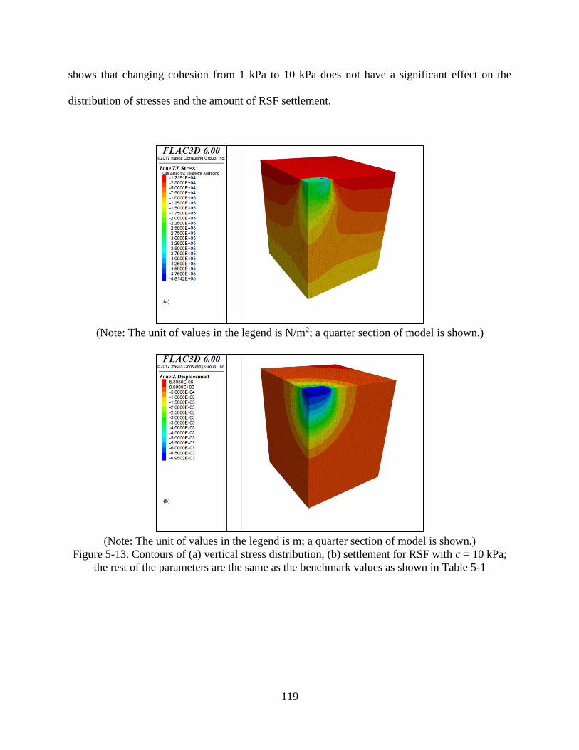
119

shows that changing cohesion from 1 kPa to 10 kPa does not have a significant effect on the

distribution of stresses and the amount of RSF settlement.



Figure 5-13. Contours of (a) vertical stress distribution, (b) settlement for RSF with c = 10 kPa;


120

Figure 5-14. Vertical stress beneath center and corner of foundation for RSF with c = 10 kPa; the


Effects of Reinforcement Stiffness


beneath the center and corner of foundation along depth for the RSF model with J = 500 kN/m.

Figures 5-17 and 5-18 show the corresponding plots for the RSF model with J = 3000 kN/m. A

comparison among Figures 5-7 and 5-8 (benchmark model) and Figures 5-15 to 5-18 shows that

under the equivalent foundation pressure of 400 kPa, the reinforcement stiffness does not have a

significant effect on the distribution of stresses and the amount of RSF settlement. However,

using a reinforcement with higher stiffness slightly increases the stresses at the corner of the

foundation.

0

1

2

3

4

0 100 200 300 400

Dep

th (

m)


Geostatic stress



121




kN/m; the rest of the parameters are the same as the benchmark values as shown in Table 5-1

122

Figure 5-16. Vertical stress beneath center and corner of foundation for RSF with J = 500 kN/m;



0

1

2

3

4

0 100 200 300 400

Dep

th (

m)


Geostatic stress



123




Figure 5-18. Vertical stress beneath center and corner of foundation for RSF with J = 3000


Effects of Reinforcement Extended Length


beneath the center and corner of foundation along depth for the RSF model with Lx = 0.25B.

Figures 5-21 and 5-22 show the corresponding plots for the RSF model with Lx = B. A

0

1

2

3

4

0 100 200 300 400

Dep

th (

m)


Geostatic stress



124


under the equivalent foundation pressure of 400 kPa the reinforcement length does not have a

significant effect on the distribution of stresses and the amount of RSF settlement.



Figure 5-19. Contours of (a) vertical stress distribution, (b) settlement for RSF with Lx=0.25B;


125

Figure 5-20. Vertical stress beneath center and corner of foundation for RSF with Lx=0.25B; the



0

1

2

3

4

0 100 200 300 400

Dep

th (

m)


Geostatic stress



126


Figure 5-21. Contours of (a) vertical stress distribution, (b) settlement for RSF with Lx=B; the


Figure 5-22. Vertical stress beneath center and corner of foundation for RSF with Lx = B; the rest


Effects of Reinforcement Spacing


beneath the center and corner of foundation along depth for the RSF model with Sv = 0.2 m.

Figures 5-25 and 5-26 show the corresponding plots for the RSF model with Sv = 0.4 m. A

0

1

2

3

4

0 100 200 300 400

Dep

th (

m)


Geostatic stress



127


within the RSF depth, the stress beneath the center of foundation with Sv = 0.4 m is higher than

the model with Sv = 0.2 m while the stress beneath the corner is smaller for the model with Sv =

0.4 m.





128

Figure 5-24. Vertical stress beneath center and corner of foundation for RSF with Sv = 0.2m; the



0

1

2

3

4

0 100 200 300 400

Dep

th (

m)


Geostatic stress



129




Figure 5-26. Vertical stress beneath center and corner of foundation for RSF with Sv = 0.4m; the


Effects of Number of Reinforcement Layers


beneath the center and corner of foundation along depth for the RSF model with N = 2. Figures

5-29 and 5-30 show the corresponding plots for the RSF model with N = 5. Since the

0

1

2

3

4

0 100 200 300 400

Dep

th (

m)


Geostatic stress



130

reinforcement spacing is the same for these cases (Sv = 0.3 m), the depth of RSF is different. A


increasing the number of reinforcement layers decreases the RSF settlement but increases the

stress concentration near the top of the compacted fill.



Figure 5-27. Contours of (a) vertical stress distribution, (b) settlement for RSF with N=2; the rest


131

Figure 5-28. Vertical stress beneath center and corner of foundation for RSF with N=2; the rest



0

1

2

3

4

0 100 200 300 400

Dep

th (

m)


Geostatic stress



132


Figure 5-29. Contours of (a) vertical stress distribution, (b) settlement for RSF with N=5; the rest


Figure 5-30. Vertical stress beneath center and corner of foundation for RSF with N=5; the rest


Effects of Width of Foundation


beneath the center and corner of foundation along depth for the RSF model with B = 3 m. A

comparison among Figures 5-7 and 5-8 (benchmark model) and Figures 5-31 and 5-32 shows

0

1

2

3

4

0 100 200 300 400

Dep

th (

m)


Geostatic stress



133

that increasing the foundation dimension increases the amount of vertical stress distribution

along the depth. For the benchmark case, the vertical stress decreases sharply after the depth of

0.6 m and the difference between the stress beneath the center and the initial stress at the depth

of 3.5 m is about 17%. For the RSF with B = 3 m, the maximum vertical stress occurs at the

depth of 1.3 m and the difference between the stress beneath the center and the initial stress at

the depth of 3.5 m is about 235%. Therefore, more attention should be paid to native soil

settlement when a foundation with large dimensions is used.


134


Figure 5-31. Contours of (a) vertical stress distribution, (b) settlement for RSF with B = 3 m; the


Figure 5-32. Vertical stress beneath center and corner of foundation for RSF with B = 3 m; the


Effects of Length of Foundation


beneath the center and corner of foundation along depth for the RSF model when L = B. Figures

5-35 and 5-36 show the corresponding plots for the RSF model with L = 10 B. A comparison

0

1

2

3

4

0 100 200 300 400

Dep

th (

m)


Geostatic stress



135

among Figures 5-7 and 5-8 (benchmark model) and Figures 5-33 to 5-34 shows that the

foundation length does not have a significant effect on the maximum stress under the foundation

but affects the distribution of stress along depth. For the RSF model with L = 10 B, the stress

decreases more gradually with depth.



Figure 5-33. Contours of (a) vertical stress distribution, (b) settlement for RSF with L=B; the rest


136

Figure 5-34. Vertical stress beneath center and corner of foundation for RSF with L=B; the rest



0

1

2

3

4

0 100 200 300 400

Dep

th (

m)


Geostatic stress



137


Figure 5-35. Contours of (a) vertical stress distribution, (b) settlement for RSF with L=10B; the


Figure 5-36. Vertical stress beneath center and corner of foundation for RSF with L=10B; the


5.7 SUMMARY


settlement of RSF. Validation of the prediction equations suggests that the prediction models

have good accuracy in estimating the immediate settlement of RSF under surcharge pressures. It

0

1

2

3

4

0 100 200 300 400

Dep

th (

m)


Geostatic stress



138

should be noted that the prediction equations for RSF settlement are based on condition that the

RSF is on a native soil of fixed thickness and fixed geotechnical properties. Distributions of

lateral deformations, settlement, and vertical stresses within the depth of the RSF of various

configurations also reveal the effects of different parameters on the performances of RSF.

139

Chapter 6. Evaluating Secondary Deformations of GRS Abutment and RSF

This chapter presents the methodology for evaluating the time-dependent, long-term deformation

(also known as creep) of GRS abutment and RSF. The creep behaviors of backfill soils and

geosynthetic reinforcement are modeled. To model the creep behavior of the backfill material,

the Burgers creep viscoplastic model combining the Burgers model and the Mohr-Coulomb

model was used in the simulations. To model the creep behavior of geosynthetics, the model

proposed by Karpurapu and Bathurst (1995) was used; this model uses a hyperbolic load-strain

function to calculate the stiffness of the reinforcement. A full-scale GRS pier loading test

conducted by Adams and Nicks (2014) was used to calibrate the creep model. Deformations of

GRS abutment and RSF with time (such as 10 years and 30 years) under various conditions are

presented in graphs.

6.1 Model Development for Long-Term Behaviors of GRS Abutment and RSF

To evaluate the time-dependent behavior of engineered fills for bridge support (i.e., GRS

abutment and RSF), the creep behavior of backfill soil and geosynthetics should be considered.

To achieve this, the Burgers creep model available in FLAC3D software was used to simulate the

long-term behavior of backfill soil. To simulate the creep behavior of geosynthetics material, the

FISH subroutine developed in the FLAC3D model (Section 3.3.2) was used.

140

6.1.1 Creep Behavior of Backfill Soil

To model the creep behavior of backfill material, the Burgers creep viscoplastic model

combining the Burgers model and the Mohr-Coulomb model was used in the simulations. The

Burgers model is composed of a Kelvin model and a Maxwell model connected in series (Figure

6-1). The Burgers creep viscoplastic model has a visco-elasto-plastic deviatoric behavior and an

elasto-plastic volumetric behavior. The viscoelastic component corresponding to the Burgers

model and the elasto-plastic component corresponding to the Mohr-Coulomb model are assumed

to act in series. The strain rate of this model is calculated using the following equation. Kelvin,

Maxwell and plastic strain contributions are labeled using the superscripts .𝐾, .𝑀, .𝑃, respectively.

�̇�𝑖𝑗 = �̇�𝑖𝑗𝐾 + �̇�𝑖𝑗

𝑀 + �̇�𝑖𝑗𝑃 (6-1)

Following equations govern the behavior of material in Kelvin, Maxwell and Mohr-

Coulomb sections.

Kelvin section: 𝑆𝑖𝑗 = 2𝜂𝐾�̇�𝑖𝑗𝐾 + 2𝐺𝐾𝑒𝑖𝑗

𝐾 (6-2)

Maxwell section: �̇�𝑖𝑗𝑀 =

�̇�𝑖𝑗

2𝐺𝑀 +𝑆𝑖𝑗

2𝜂𝑀 (6-3)

Mohr-Coulomb section: �̇�𝑖𝑗𝑃 = 𝜆∗ 𝜕𝑔

𝜕𝜎𝑖𝑗−

1

3�̇�𝑣𝑜𝑙

𝑃 𝛿𝑖𝑗 (6-4)

�̇�𝑣𝑜𝑙𝑃 = 𝜆∗ [

𝜕𝑔

𝜕𝜎11+

𝜕𝑔

𝜕𝜎22+

𝜕𝑔

𝜕𝜎33] (6-5)

The model uses bulk modulus, cohesion, friction angle, dilation angle, unit weight,

Kelvin shear modulus, Kelvin viscosity, Maxwell shear modulus, and Maxwell viscosity as the

input parameters. The elastic modulus, cohesion, friction angle and dilation angle of the backfill

soil are the same as those used in the previous numerical simulations in Chapters 4 and 5. The

Maxwell and Kelvin viscosities and shear moduli should be calibrated for granular materials.

141

Figure 6-1. Schematic of the Burgers model

6.1.2 Creep Behavior of Geosynthetic Reinforcement

Reinforcement materials such as biaxial geogrids, geotextiles, and metal strips are usually

modeled as linear elastic materials, as often done in past studies reported in literature (e.g.,

Kurian et al. 1997; Helwany et al. 1999; Leshchinsky and Vulova 2001; Skinner and Rowe 2003;

Chen et al. 2007; Zheng and Fox 2016). This treatment is considered sufficient because the in-

service stress level is generally low. To consider the creep behavior of geosynthetic

reinforcement and to to account for strain-dependent tensile stiffness of the reinforcement,

Karpurapu and Bathurst (1995) proposed the following equation:

(6-6)

where = reinforcement tangential stiffness; T = reinforcement axial load; = reinforcement axial

strain; A = reinforcement initial stiffness; and B = reinforcement strain softening coefficient.

Equation 6-1 was successfully used by Hatami and Bathurst (2005) to model GRS segmental

walls.

BA

d

BA

d

dTJ t 2

)()(

2

142

To model the creep behavior of geosynthetics material, Equation 6-1 proposed by Karpurapu and

Bathurst (1995) was used. A FISH subroutine was implemented in FLAC3D to update the

reinforcement stiffness automatically to account for changes of reinforcement strain with time.

This subroutine was developed in previous simulations of this study to update the reinforcement

stiffness.

6.1.3 Model Calibration

To validate the numerical model developed to predict the long-term behavior of GRS composite

materials, a large-scale experiment was selected to compare the simulation results with

experimental results. The experiment was a GRS pier loading test conducted by Adams and

Nicks (2014), in which the settlement of the pier was measured for a period of 105 days. Figure

6-2 shows the GRS pier configuration used in the long-term performance test.

Figure 6-2. GRS pier configuration used in long-term performance test

(after Adams and Nicks 2014)

The GRS pier was 1.2 m square with a height of 2.3 m founded on a concrete slab. The

backfill soil was a well-graded aggregate AASHTO A-1-a. A woven polypropylene geotextile

was used as the reinforcement. Table 6-1 summarizes the material properties of the GRS pier.

143

Table 6-1. GRS pier material properties Component Parameter Value

Backfill

Type A-1-a

dmax (mm) 25.4

Friction angle (°) 54

Cohesion (kPa) 5.5

Reinforcement Wide width tensile strength, Tf (kN/m) 70

MARV strength at 2% strain, Tε=2% (kN/m) 19.3

An approach similar to that described in Section 3.6.4 was used to simulate the

construction process and the performance of the GRS pier under the surcharge load of 210 kPa.

To evaluate the long-term performance of the pier, the Burgers model combined with the Mohr-

Coulomb model was used to simulate the visco-plastic behavior of backfill. The bulk modulus

obtained at the equilibrium state under the 210 kPa applied pressure was used as the input bulk

modulus for the long-term simulation. The Burgers model parameters used in this simulation are

presented in Table 6-2. Equation 3-3 proposed by Karpurapu and Bathurst (1995) was used to

simulate the long-term behavior of reinforcement. During the simulation, the reinforcement

stiffness was updated based on the reinforcement strain. The two following equations were used

to calculate the reinforcement stiffness.

𝐽𝑡(휀) = 1250 − 19580 × 휀 [kN/m] 0 < ε < 0.02 (6-7)

𝐽𝑡(휀) = 912 − 2676 × 휀 [kN/m] 0.02 < ε < 0.08 (6-8)

The experimental and numerical time-settlement results of this test are illustrated in

Figure 6-3, which shows that the numerical model with the calibrated parameters shown in Table

6-2 had a good ability in predicting the long-term behavior of GRS composite.

144

Table 6-2. Burgers model parameters Maxwell shear modulus

(Pa )

Maxwell viscosity

(Pa ·s)

Kelvin shear modulus

(Pa )

Kelvin viscosity

(Pa·s )

4×107 5×1015 1×109 6×1011

Figure 6-3. Experimental and numerical time-settlement results of the GRS pier

6.2. Long-Term Behavior of GRS Abutment

To evaluate the long-term behavior of GRS abutment the same approach explained in the

previous section was used for simulating the creep behavior of the backfill soil and the

reinforcement. In this study, the long-term behavior of GRS abutments under an applied pressure

of 200 kPa was studied to evaluate the lateral and vertical deformations of these structures during

10 years and 30 years of service life. The same Burgers parameters from Table 6-2 were used for

granular backfill material; however, the bulk modulus, density and the Mohr-Coulomb

parameters (e.g., friction angle, dilation angle and cohesion) differed for different backfill soils

that were evaluated.

0

5

10

15

20

25

30

0 40 80 120

Set

tlem

ent

(mm

)

Time (Days)

Experiment

Simulation

145

6.2.1 Benchmark Model

In the first study, the long-term performance of GRS abutment with the benchmark values

summarized in Table 6-3 was evaluated during 30 years of service life under 200 kPa applied

pressure. The lateral deformation, settlement and vertical stress distribution contours for the

benchmark model when 200 kPa pressure was applied on the foundation, and after 10 and 30

years of applying the load are presented in Figures 6-4 to 6-6. Over time, the amount of lateral

deformation, settlement and the vertical stress at the toe of GRS abutment increased. The

locations of maximum deformations and vertical stress were almost the same over time.

However, after 30 years, the relative amount of backfill settlement behind the foundation and the

lateral deformation of the toe of abutment increased noticeably.

Table 6-3. Benchmark values for GRS abutment models

Parameters Benchmarks Values

Friction angle, () 48

Reinforcement length, (m) 2.5

Reinforcement initial stiffness, (kN/m) 2000

Reinforcement spacing, (m) 0.2

Abutment height, (m) 5

Facing batter, () 2


RL

J

vS

H

146



Figure 6-4. Contours of (a) lateral deformation, (b) settlement, and (c) vertical stress distribution

of benchmark model immediately after applying 200 kPa pressure

147


of benchmark model after 10 years of applying 200 kPa

148


of benchmark model after 30 years of applying 200 kPa

149

Figures 6-7 and 6-8 show the lateral deformation and settlement of GRS abutment using the

benchmark values in 30 years, respectively. These figures indicate that the majority of the

abutment final deformations occurred within the first year. Table 6-4 summarized the GRS

abutment deformations after 1 month, 1 year, 5, 10, and 30 years and the ratios of these

deformations to the initial value after applying 200 kPa pressure.

Figure 6-7. Lateral deformation of benchmark model under 200 kPa pressure: (a) normal

timescale; (b) logarithmic timescale

5

6

7

8

9

10

0 10 20 30 40

Lat

eral

def

orm

atio

n (

mm

)

Time (year)

Secondary deformation

Immediate deformation

5

6

7

8

9

10

0.001 0.01 0.1 1 10 100

Lat

eral

def

orm

atio

n (

mm

)

Time (year)

(b)

150

Figure 6-8. Settlement of benchmark model under 200 kPa pressure: (a) normal timescale; (b)

logarithmic timescale

Table 6-4. Deformations of benchmark GRS abutment with time

Time Lateral Deformation Settlement

(mm) /0 (mm) /0

Immediate (0 or

0) 7.3 1.00 11.30 1.00

1 Month 8.76 1.20 13.05 1.15

1 Year 8.92 1.22 13.14 1.16

5 Years 9.06 1.24 13.32 1.18

10 years 9.33 1.28 13.54 1.20

30 years 9.76 1.34 13.92 1.23

10

11

12

13

14

15

0 5 10 15 20 25 30 35

Set

tlem

ent

(mm

)

Time (year)

Secondary settlement

Immediate settlement

10

11

12

13

14

15

0.0001 0.001 0.01 0.1 1 10 100

Set

tlem

ent

(mm

)

Log time (year)

(b)

151

6.2.2 Effect of Reinforcement Spacing

The long-term performance of GRS abutments with the reinforcement spacing of 0.8 m was

evaluated during 10 years of service life under 200 kPa applied pressure. Figures 6-13 and 6-14

show the lateral deformation and settlement of GRS abutment with Sv = 0.8 m within 10 years

while keeping the rest of the parameters the same as the benchmark model. Table 6-6

summarizes the abutment deformations after 1 month, 1 year, 5 years and 10 years. A

comparison among Table 6-4 (benchmark case) and Table 6-6 shows that as the reinforcement

spacing increases, the ratio of the secondary deformation to the immediate deformation

increases. The comparison shows that, over time, different reinforcement spacing (0.2 m vs. 0.8

m) yields similar ratio of secondary lateral deformation (28% vs. 26%) relative to the immediate

deformation; but more closely-spaced reinforcement tends to yield less secondary settlement

relative to its immediate settlement. After 10 years, the secondary lateral deformation ranges

from 26% to 28% of the immediate lateral deformation, and the secondary settlement ranges

from 20% to 30% of the immediate settlement for the reinforcement spacing ranging from 0.2 m

to 0.8 m.

Figure 6-13. Lateral deformation of GRS abutment with Sv = 0.8 m under 200 kPa pressure: (a)


benchmark values as shown in Table 6-3

30

33

36

39

42

0 5 10

Lat

eral

def

orm

atio

n (

mm

)

Time (year)



30

33

36

39

42

0.001 0.01 0.1 1 10

Lat

eral

def

orm

atio

n (

mm

)

Time (year)

152

Figure 6-14. Settlement of GRS abutment with Sv = 0.8 m under 200 kPa pressure: (a) normal


values as shown in Table 6-3

Table 6-6. Time-dependent deformations of GRS abutment with Sv = 0.8 m


(mm) /0 (mm) /0

Immediate (for 0

or 0) 31.46 1.00 31.40 1.00

1 Month 36.36 1.16 36.51 1.16

1 Year 39.12 1.24 40.12 1.28

5 Years 39.37 1.25 40.44 1.29

10 years 39.77 1.26 40.67 1.30

6.2.3 Effect of Reinforcement Length

The long-term performances of GRS abutments with LR=H were evaluated during 10 years of

service life under 200 kPa applied pressure. Figures 6-15 and 6-16 show the lateral deformation

and settlement of the GRS abutment with LR=H during 10 years while keeping the rest of the

parameters the same as the benchmark model. Table 6-7 summarizes the abutment deformations

after 1 month, 1 year, 5 years and 10 years. A comparison among Table 6-4 (benchmark case)

and Table 6-7 shows that as the length of reinforcement increases, the ratio of the secondary

deformation to the immediate deformation decreases. This shows that, over time, a GRS

abutment with a longer reinforcement length tends to have less displacement relative to its initial

30

33

36

39

42

0 5 10S

ettl

emen

t (m

m)

Time (year)

(a)



30

33

36

39

42

0.01 0.1 1 10

Set

tlem

ent

(mm

)

Time (year)

(b)

153

displacement. It suggests that the long-term deformation of GRS abutments may be reduced by

increasing the reinforcement length. After 10 years, the secondary lateral deformation ranges

from 18% to 28% of the immediate lateral deformation, and the secondary settlement ranges

from 17% to 20% of the immediate settlement for LR ranging from 2.5 m (0.5H) to 5 m (H).

Figure 6-15. Lateral deformation of GRS abutment with LR=H under 200 kPa pressure: (a)



Figure 6-16. Settlement of GRS abutment with LR=H under 200 kPa pressure: (a) normal



6

7

8

9

0 5 10

Lat

eral

def

orm

atio

n (

mm

)

Time (year)



6

7

8

9

0.01 0.1 1 10

Lat

eral

def

orm

atio

n (

mm

)

Time (year)

10

11

12

13

14

0 5 10

Set

tlem

ent

(mm

)

Time (year)

(a)



10

11

12

13

14

0.001 0.01 0.1 1 10

Set

tlem

ent

(mm

)

Time (year)

(b)

154

Table 6-7. Time-dependent deformations of GRS abutment with LR=H


(mm) /0 (mm) /0

Immediate (for 0

or 0) 6.90 1.00 11.30 1.00

1 Month 7.68 1.11 12.66 1.12

1 Year 7.80 1.13 12.79 1.13

5 Years 7.94 1.15 12.95 1.15

10 years 8.15 1.18 13.18 1.17

6.2.4 Effect of Reinforcement Stiffness

The long-term performances of GRS abutments with reinforcement stiffness of 500 kN/m were

evaluated during 10 years of service life under 200 kPa applied pressure. Figures 6-17 and 6-18

show the lateral deformation and settlement of the GRS abutment with J = 500 kN/m during 10

years while keeping the rest of the parameters the same as the benchmark model. Table 6-8

summarizes the abutment deformations after 1 month, 1 year, 5 years and 10 years. A

comparison among Table 6-4 (benchmark case) and Table 6-8 shows that, after 10 years,

different reinforcement stiffness (2000 kN/m vs. 500 kN/m) yields similar ratio of secondary

lateral deformation (28% vs. 24%) relative to the immediate lateral deformation; but higher

reinforcement stiffness tends to yield less settlement relative to its initial settlement. After 10

years, the secondary lateral deformation ranges from 24% to 28% of the immediate lateral

deformation, and the secondary settlement ranges from 20% to 35% of the immediate settlement

for the reinforcement stiffness ranging from 500 kN/m to 200 kN/m.

155

Figure 6-17. Lateral deformation of GRS abutment with J = 500 kN/m under 200 kPa pressure:

(a) normal timescale; (b) logarithmic timescale; the rest of the parameters are the same as the


Figure 6-18. Settlement of GRS abutment with J = 500 kN/m under 200 kPa pressure: (a) normal



Table 6-8. Time-dependent deformations of GRS abutment with J = 500 kN/m


(mm) /0 (mm) /0

Immediate (for 0 or

0) 15.90 1.00 21.70 1.00

1 Month 17.72 1.11 24.00 1.11

1 Year 19.32 1.22 28.88 1.33

5 Years 19.50 1.23 29.12 1.34

10 years 19.70 1.24 29.24 1.35

15

17

19

21

0 5 10

Lat

eral

def

orm

atio

n (

mm

)Time (year)

(a)Secondary deformation


15

18

21

0.01 0.1 1 10

Lat

eral

def

orm

atio

n (

mm

)

Time (year)

(b)

20

23

26

29

32

0 5 10

Set

tlem

ent

(mm

)

Time (year)

(a)



20

23

26

29

32

0.01 0.1 1 10

Set

tlem

ent

(mm

)

Time (year)

(b)

156

6.2.5 Effect of Abutment Height

The long-term performances of GRS abutments with a height of 3 m and 9 m were evaluated

during 10 years of service life under 200 kPa applied pressure. Figures 6-19 and 6-20 show the

lateral deformation and settlement of GRS abutment with H = 3 m during 10 years while keeping

the rest of the parameters the same as the benchmark model. Figures 6-21 and 6-22 show the

lateral deformation and settlement for the GRS model with H = 9 m. Table 6-9 summarizes the

abutments deformations after 1 month, 1 year, 5 years and 10 years for these cases. A

comparison among Table 6-4 (benchmark case) and Table 6-9 does not show a clear trend of

how the abutment height affects the long-term behavior of GRS abutment. For example, the

abutment heights of 3 m, 5 m, and 9 m yield secondary lateral deformation of 33%, 28%, and

48% of the immediate lateral deformation, respectively, and secondary settlement of 22%, 20%,

and 26% of immediate settlement, respectively. A possible reason is that in addition to the

abutment height, the length of the reinforcement also varies in these cases since LR = 0.5 H. But

the results clearly show that abutment height affects the secondary deformations. After 10 years,

the secondary lateral deformation ranges from 33% to 48% of the immediate lateral deformation,

and the secondary settlement ranges from 22% to 26% of the immediate settlement for the

abutment height ranging from 3 m to 9 m.

157

Figure 6-19. Lateral deformation of GRS abutment with H= 3 m under 200 kPa pressure: (a)



Figure 6-20. Settlement of GRS abutment with H= 3 m under 200 kPa pressure: (a) normal



4

6

8

10

0 5 10

Lat

eral

def

orm

atio

n (

mm

)Time (year)



4

6

8

10

0.01 0.1 1 10

Lat

eral

def

orm

atio

n (

mm

)

Time (year)

(b)

8

10

12

0 5 10

Set

tlem

ent

(mm

)

Time (year)

(a)



8

10

12

0.01 0.1 1 10

Set

tlem

ent

(mm

)

Time (year)

(b)

158

Figure 6-21. Lateral deformation of GRS abutment with H=9 m under 200 kPa pressure: (a)



Figure 6-22. Settlement of GRS abutment with H=9 m under 200 kPa pressure: (a) normal



8

10

12

14

16

0 5 10

Lat

eral

def

orm

atio

n (

mm

)Time (year)



8

10

12

14

16

0.01 0.1 1 10

Lat

eral

def

orm

atio

n (

mm

)

Time (year)

16

18

20

22

24

0 5 10

Set

tlem

ent

(mm

)

Time (year)

(a)



16

18

20

22

24

0.0001 0.01 1

Set

tlem

ent

(mm

)

Time (year)

(b)

159

Table 6-9. Time-dependent deformations of GRS abutment with different heights

Height

value Time

Lateral Deformation Settlement

(mm) /0 (mm) /0

3 m

Immediate (for 0 or

0) 5.70 1.00 9.20 1.00

1 Month 6.42 1.13 10.04 1.09

1 Year 7.39 1.30 11.00 1.20

5 Years 7.49 1.31 11.12 1.21

10 years 7.61 1.33 11.23 1.22

9 m

Immediate (for 0 or

0) 9.60 1.00 17.20 1.00

1 Month 10.92 1.14 19.69 1.14

1 Year 13.39 1.40 20.68 1.20

5 Years 13.75 1.43 21.03 1.22

10 years 14.19 1.48 21.60 1.26

6.2.6 Effect of Facing Batter

The long-term performances of GRS abutments with a facing batter of 0° and 4° were evaluated

during 10 years of service life under 200 kPa applied pressure. Figures 6-23 and 6-24 show the

lateral deformation and settlement of GRS abutment with = 0° during 10 years while keeping

the rest of the parameters the same as the benchmark model. Figures 6-25 and 6-26 show the

lateral deformation and settlement for the GRS mode with = 4°. Table 6-10 summarizes the

abutment deformations after 1 month, 1 year, 5 years and 10 years for these cases. A comparison

among Table 6-4 (benchmark case) and Table 6-10 shows that as the facing batter increases, the

ratio of the secondary deformation to the immediate deformation decreases. After 10 years, the

secondary lateral deformation ranges from 23% to 46% of the immediate lateral deformation; the

secondary settlement ranges from 18% to 25% of the immediate settlement for the facing batter

ranging from 0° to 4°.

160

Figure 6-23. Lateral deformation of GRS abutment with = 0 under 200 kPa pressure: (a)



Figure 6-24. Settlement of GRS abutment with = 0 under 200 kPa pressure: (a) normal



8

10

12

14

0 5 10

Lat

eral

def

orm

atio

n (

mm

)Time (year)



8

10

12

14

0.0001 0.01 1

Lat

eral

def

orm

atio

n (

mm

)

Time (year)

(b)

11

12

13

14

15

16

0 5 10

Set

tlem

ent

(mm

)

Time (year)

(a)Secondary settlement


11

12

13

14

15

16

0.00001 0.001 0.1 10

Set

tlem

ent

(mm

)

Time (year)

(b)

161

Figure 6-25. Lateral deformation of GRS abutment with = 4° under 200 kPa pressure: (a)



Figure 6-26. Settlement of GRS abutment with = 4° under 200 kPa pressure: (a) normal



4

5

6

7

8

0 5 10

Lat

eral

def

orm

atio

n (

mm

)Time (year)



4

5

6

7

8

0.001 0.01 0.1 1 10

Lat

eral

def

orm

atio

n (

mm

)

Time (year)

(b)

10

11

12

13

14

0 2 4 6 8 10

Set

tlem

ent

(mm

)

Time (year)

(a) Secondary settlement


10

11

12

13

14

0.001 0.01 0.1 1 10

Set

tlem

ent

(mm

)

Time (year)

(b)

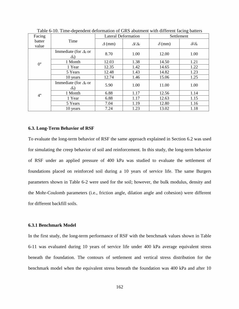
162

Table 6-10. Time-dependent deformation of GRS abutment with different facing batters Facing

batter

value

Time

Lateral Deformation Settlement

(mm) /0 (mm) /0

0°

Immediate (for 0 or

0) 8.70 1.00 12.00 1.00

1 Month 12.03 1.38 14.50 1.21

1 Year 12.35 1.42 14.65 1.22

5 Years 12.48 1.43 14.82 1.23

10 years 12.74 1.46 15.06 1.25

4°

Immediate (for 0 or

0) 5.90 1.00 11.00 1.00

1 Month 6.88 1.17 12.56 1.14

1 Year 6.88 1.17 12.63 1.15

5 Years 7.04 1.19 12.80 1.16

10 years 7.24 1.23 13.02 1.18

6.3. Long-Term Behavior of RSF

To evaluate the long-term behavior of RSF the same approach explained in Section 6.2 was used

for simulating the creep behavior of soil and reinforcement. In this study, the long-term behavior

of RSF under an applied pressure of 400 kPa was studied to evaluate the settlement of

foundations placed on reinforced soil during a 10 years of service life. The same Burgers

parameters shown in Table 6-2 were used for the soil; however, the bulk modulus, density and

the Mohr-Coulomb parameters (i.e., friction angle, dilation angle and cohesion) were different

for different backfill soils.

6.3.1 Benchmark Model

In the first study, the long-term performance of RSF with the benchmark values shown in Table

6-11 was evaluated during 10 years of service life under 400 kPa average equivalent stress

beneath the foundation. The contours of settlement and vertical stress distribution for the

benchmark model when the equivalent stress beneath the foundation was 400 kPa and after 10

163

years are presented in Figures 6-27 and 6-28. Over time, the amount of secondary settlement of

RSF increased, the maximum vertical stress remained the same, but the stress distribution and

the location of the maximum stress have changed.

Table 6-11. Benchmark values for RSF models

Parameters Benchmarks values

Friction angle, () 40

Cohesion, (kPa) 1

Reinforcement spacing, (m) 0.3

Number of reinforcement layers, N 3

Reinforcement initial stiffness, (kN/m) 1000

Width of foundation, (m) 1

Length of foundation, L (m) 2 B


c

vS

J

B

164



RSF immediately after loading; the equivalent stress at the bottom of foundation is 400 kPa

165


RSF after 10 years of applying 400 kPa of equivalent foundation stress

Figures 6-29 shows the total settlement of foundation placed on RSF within 10 years. The figure

indicates that a large percentage of the foundation settlement occurred within the first year. Table

6-12 summarizes the RSF settlement after 1 month, 1 year, 5 years and 10 years and the ratios of

these settlements to the initial value when the equivalent stress beneath the foundation was 400

kPa.

6

8

10

12

14

0 2 4 6 8 10

Set

tlem

ent

(mm

)

Time (year)



166

Figure 6-29. Total settlement of benchmark model under 400 kPa of equivalent foundation

pressure; (a) normal timescale; (b) logarithmic timescale

Table 6-12. Time-dependent settlement for the benchmark RSF

Time Settlement

(mm) /0

Immediate (0) 7.76 1.00

1 Month 8.89 1.15

1 Year 12.02 1.55

5 Years 12.40 1.60

10 years 12.66 1.63

6.3.2 Effect of reinforcement stiffness

The long-term performances of RSF with the reinforcement stiffness of 500 kN/m and 3000

kN/m were evaluated during 10 years of service life under 400 kPa of equivalent foundation

pressure. Figures 6-33 and 6-34 show the settlement of RSF with J = 500 kN/m and J = 3000

kN/m within 10 years, respectively, while keeping the rest of the parameters the same as the

benchmark model. Table 6-13 summarizes the total settlement of foundation after 1 month, 1

year, 5 years and 10 years for these cases. A comparison among Table 6-12 (benchmark case)

and Table 6-15 shows that reinforcement stiffness does not affect the long-term settlement of

6

8

10

12

14

0.01 0.1 1 10

Set

tlem

ent

(mm

)

Time (year)

(b)

167

RSF. For example, the reinforcement stiffness of 500 kN/m, 1000 kN/m, and 3000 kN/m all

yields the same ratio of the secondary settlement to the immediate settlement (i.e., 63%).

Figure 6-33. Total settlement of RSF with J = 500 kN/m under 400 kPa of equivalent foundation


as the benchmark values as shown in Table 6-11

Figure 6-34. Total settlement of RSF with J = 3000 kN/m under 400 kPa of equivalent

foundation pressure: (a) normal timescale; (b) logarithmic timescale; the rest of the parameters

are the same as the benchmark values as shown in Table 6-11

6

8

10

12

14

0 5 10

Set

tlem

ent

(mm

)

Time (year)



6

8

10

12

14

0.01 0.1 1 10

Set

tlem

ent

(mm

)

Time (year)

(b)

6

8

10

12

14

0 5 10

Set

tlem

ent

(mm

)

Time (year)



6

8

10

12

14

0.01 0.1 1 10

Set

tlem

ent

(mm

)

Time (year)

(b)

168

Table 6-15. Time-dependent settlement for RSF with different reinforcement stiffness

Reinforcement

stiffness Time

Settlement

(mm) /0

500 kN/m

Immediate (0 or 0) 7.86 1.00

1 Month 10.18 1.30

1 Year 12.66 1.61

5 Years 12.82 1.63

10 years 12.85 1.63

3000 kN/m

Immediate (0 or 0) 7.68 1.00

1 Month 9.09 1.18

1 Year 11.79 1.54

5 Years 12.41 1.62

10 years 12.53 1.63

6.3.3 Effect of Number of reinforcement layers

The long-term performances of RSF with 2 and 5 layers of reinforcement were evaluated during

10 years of service life under 400 kPa of equivalent foundation pressure. Figures 6-35 and 6-36

show the settlement of RSF with N=2 and N=5 within 10 years, respectively, while keeping the

rest of the parameters the same as the benchmark model. Table 6-16 summarizes the total

settlement of foundation after 1 month, 1 year, 5 years and 10 years for these cases. A

comparison among Table 6-12 (benchmark case) and Table 6-16 shows that as the number of

reinforcement layers increases, the ratio of the secondary settlement to the immediate settlement

also increases. A possible reason is that, by having the same reinforcement spacing (0.3 m), the

depth of RSF is greater for the case with more layers of reinforcements, this can lead to higher

secondary settlement. After 10 years, the secondary settlement ranges from 57% to 71% of the

immediate settlement of RSF for the number of reinforcement layers ranging from 2 to 5.

169







7

10

13

16

0 5 10

Set

tlem

ent

(mm

)Time (year)



7

10

13

16

0.01 0.1 1 10

Set

tlem

ent

(mm

)

Time (year)

(b)

5

8

11

14

0 5 10

Set

tlem

ent

(mm

)

Time (year)



5

8

11

14

0.001 0.01 0.1 1 10

Set

tlem

ent

(mm

)

Time (year)

(b)

170

Table 6-16. Time-dependent settlement for RSF with different numbers of reinforcement layers

Number of

reinforcement layers Time

Settlement

(mm) /0

2

Immediate (0 or 0) 8.78 1.00

1 Month 12.12 1.38

1 Year 12.81 1.46

5 Years 13.27 1.51

10 years 13.74 1.57

5

Immediate (0 or 0) 6.66 1.00

1 Month 9.55 1.43

1 Year 11.15 1.67

5 Years 11.31 1.70

10 years 11.38 1.71

6.5 Summary

A numerical model was developed to investigate the time-dependent deformations of GRS

abutment and RSF; the time-dependent deformations are also known as secondary deformations

and creep.

The creep model results on GRS abutment show that (1) after 10 years, the secondary

lateral deformation of GRS abutment with various configurations ranges from 15% to 54% of the

immediate lateral deformation, and the secondary settlement of GRS abutment with various

configurations ranges from 14% to 35% of the immediate settlement; (2) different reinforcement

spacing yields similar ratio of secondary lateral deformation relative to the immediate

deformation, but more closely-spaced reinforcement tends to yield less settlement relative to its

immediate settlement; (3) increasing the reinforcement length reduces the long-term deformation

of GRS abutments; (4) different reinforcement stiffness (2000 kN/m vs. 500 kN/m) yields similar

ratio of secondary lateral deformation relative to the immediate lateral deformation, but higher

reinforcement stiffness tends to yield less settlement relative to its initial settlement; (6) although

a clear relationship between abutment height and secondary deformation was not obtained, the

171

model results clearly show that abutment height affects the secondary deformations; and (7) as

the facing batter increases, the ratio of the secondary deformation to the immediate deformation

decreases..

The creep model results on RSF show that (1) after 10 years, the secondary settlement of

RSF of various configurations ranges from 57% to 118% of the immediate settlement of RSF;

(2) over time, the amount of secondary settlement of RSF increased, the maximum vertical stress

remained the same, but the stress distribution and the location of the maximum stress have

changed; and (3) reinforcement stiffness does not affect the long-term settlement of RSF.

172

Chapter 7. Summary and Conclusions

7.1 Summary

This dissertation presents design tools for the service limit state (SLS) design of geosynthetic

reinforced soil (GRS) bridge abutment and reinforced soil foundation (RSF) as well as analyses

of the factors that affect the SLS of these bridge supports. The SLS includes settlement and

lateral deformation immediately after the construction and time-dependent deformation that is

also known as creep. The finite difference-based program FLAC3D 6.0 (Fast Lagrangian Analysis

of Continua) was used to conduct numerical analyses of engineered fills for bridge support. The

numerical model adopted constitutive models for compacted engineered fills and foundation

soils, reinforcement materials and facing units, and soil-reinforcement interaction. The

parameters in the developed models were calibrated and validated using three case studies.

Comparisons of the model results and the reported results in the case studies showed the models

can appropriately predict the performances of GRS piers, GRS abutment and retaining walls, and

shallow foundations on reinforced soils. The design tools are prediction equations that were

derived from numerical simulations and regression analyses of the simulation results. The best

prediction equations for GRS abutment and RSF deformations that have the least root mean

square error (RMSE) value and the highest coefficient of determination (R2) value were

suggested. Stress distributions within the engineered fills of the GRS abutment and RSF were

also presented.

The creep behaviors of backfill soils and geosynthetic reinforcement were modeled. To

model the creep behavior of the backfill material, the Burgers creep viscoplastic model combined

with the Burgers model and the Mohr-Coulomb model was used in the simulations. To model the

173

creep behavior of geosynthetics, the model proposed by Karpurapu and Bathurst (1995) was

used; this model uses a hyperbolic load-strain function to calculate the stiffness of the

reinforcement. A full-scale GRS pier loading test conducted by Adams and Nicks (2014) was

used to calibrate the creep model. Deformations of GRS abutment and RSF with time (such as 10

years and 30 years) under various influencing parameters are presented in graphs.

7.2 Conclusions

In this research the impact of various soil constitutive models was evaluated. Three different

constitutive models were used to simulate the backfill soil: the elastic-perfectly plastic Mohr-

Coulomb model, the Plastic Hardening model, and the Plastic Hardening model combined with

strain-softening behavior. Results of the numerical simulations showed that the Plastic

Hardening model can accurately predict the behavior of GRS structure under service loads.

However, at ultimate loads, only the Plastic Hardening model combined with strain-softening

behavior can accurately capture the response of GRS piers. Since the focus of this research was

on service limit state behavior of engineered fill, the Plastic Hardening model was selected as a

suitable model to simulate the behavior of backfill soil under service loads.

This study suggested Equation 4-9 for predicting the immediate maximum lateral

deformation of GRS abutment under surcharge loads with R2 = 0.91 and RMSE = 0.0043:

𝐿𝐺𝑅𝑆 = 0.056 × 𝑞∗1.32 × 𝑐𝑜𝑡2𝜙 ×𝑆𝑣

∗

𝐽∗0.17 × 𝐵∗1.11(0.16 − 1.69𝛽∗ + 0.105𝐻∗ − 0.0125𝐿𝑅∗ 2) (4-9)

This study suggested Equation 4-10 for predicting the immediate settlement of GRS

abutments under surcharge loads with R2 = 0.88 and RMSE = 0.0054:

𝑆𝐺𝑅𝑆 = 0.005 + 0.006 × 𝑞∗1.42 × 𝑐𝑜𝑡2𝜙 ×𝑆𝑣

∗

𝐽∗0.49 × 𝐵∗1.26(3.4 − 26.7𝛽∗ + 0.025𝐻∗ − 0.2𝐿𝑅∗ ) (4-10)

174

q*, Sv*, J*, *, H*, LR* and B* are defined as q/q0, Sv/ Sv0, J/J0, /0, H/H0, LR/LR0 and B/B0,

respectively. q should be in the unit of kPa, and should be in degree, J should be in the unit

of kN/m, and Sv, H, LR, and B should be in the unit of m, then LGRS and SGRS result would be in

m. In this study q0 = 200 kPa, Sv0 = 0.2 m, J0 = 500 kN/m, 0 = 90°, H0 = 5 m, LR0 =2.5 m and B0

=1 m. It should be noted that the suggested equations by this study were calibrated for GRS

abutment with friction angle between 40° and 55°, reinforcement spacing between 0.2 m and 0.8

m, reinforcement length between 0.4H and H, reinforcement stiffness between 500 kN/m and

2500 kN/m, abutment height between 3 m and 9 m, Facing batter between 0° and 8°, and

foundation width value between 0.5 m and 3 m under the vertical surcharge loads between 50

kPa and 400 kPa. Also the backfill cohesion should be negligible (around 1 kPa).

The above prediction equations are further validated using case studies. Comparisons of

the proposed equations on immediate deformations of GRS abutment and settlement of RSF with

other available methods showed that the proposed equations have a good flexibility in estimating

the deformations of cases with different conditions and have a good accuracy in predicting

deformations compared to other available methods.

The sensitivity analysis of the prediction equation of lateral deformation of GRS

abutment shows the following decreasing effect of the parameters on the lateral deformation of

GRS abutment:

(1) friction angle of backfill

(2) reinforcement spacing

(3) foundation width

(4) abutment height

(5) facing batter

175

(6) reinforcement length

(7) reinforcement initial stiffness.

The sensitivity analysis of the prediction equation of settlement of GRS abutment shows

the following decreasing effect of the parameters on the settlement of GRS abutment:


(2) foundation width


(4) abutment height

(5) reinforcement initial stiffness

(6) facing batter

(7) reinforcement length.

This study suggested the following prediction model for the total immediate settlement of

RSF:

𝑆𝑅𝑆𝐹 = 1.3 × 10−3 × 𝑞∗1.17 × 𝑐𝑜𝑡2𝜙 × 𝑁−0.05 × (−0.07 − 6.5 × 10−5𝑐∗ + 67.9(𝑆𝑣∗/𝐽∗) + 0.15𝐷𝑐

∗ +

0.06𝐵∗ + 5 × 10−4𝑙𝑜𝑔𝐿∗) (5-8)

q*, c*, J*, Sv*, Dc*, B*, L*, and Lx* are defined as q/q0, c/c0, J/J0, Sv/ Sv0, Dc/Dc0, B/B0, L/L0, and

LX/LX0 respectively. q and c should be in the unit of kPa, in degree, J in kN/m, and Sv, Dc, B, L

and LX in the unit of m, then SRSF result would be in m. In this study q0 = 100 kPa, c0 = 1 kPa, J0

= 100 kN/m, Sv0 = 0.1 m, Dc0 = 1 m, B0 = 1 m, L0 = 1 m and LX0 = 1 m. It should be noted that the

suggested equation by this study was calibrated for RSF with friction angle between 30° and 50°,

cohesion between 0 and 10 kPa, reinforcement spacing between 0.2 m and 0.4 m, number of

reinforcement between 2 and 6, compacted depth between 0.9 m and 1.8 m, reinforcement

stiffness between 500 kN/m and 3000 kN/m, foundation width between 1 m and 3 m, and

176

foundation length between 1B and 10B under the service loads of 50 kPa to 600 kPa. The above

equation is based on the foundation’s embedment depth of Df = 0.6 m. Validation of the

prediction equation suggests that the prediction model has good accuracy in estimating the

immediate settlement of RSF under surcharge load.

The sensitivity analysis of the prediction equation of total settlement of RSF shows the

following decreasing effect of the parameters on the total settlement of RSF:


(2) compacted depth


(4) reinforcement stiffness

(5) width of foundation

(6) length of foundation

(7) number of reinforcement layers

(8) cohesion of backfill.

A numerical model was developed to investigate the time-dependent deformations of

GRS abutment and RSF. The time-dependent deformations are also known as secondary

deformations and creep. The majority of the final deformations of GRS abutment and RSF occur

within the first year. It should be noted that in this study the effects of moisture content,

temperature, ageing and biological and chemical degradation on the long-term behavior of

backfill soil and reinforcement layers were not considered.

The creep model results on GRS abutment show that (1) after 10 years, the secondary

lateral deformation of GRS abutment with various configurations ranges from 15% to 54% of the

immediate lateral deformation, and the secondary settlement of GRS abutment with various

177

configurations ranges from 14% to 35% of the immediate settlement; (2) different reinforcement

spacing yields similar ratio of secondary lateral deformation relative to the immediate

deformation; but more closely-spaced reinforcement tends to yield less settlement relative to its

immediate settlement; (3) increasing the reinforcement length reduces the long-term deformation

of GRS abutments; (4) different reinforcement stiffness yields similar ratio of secondary lateral

deformation relative to the immediate lateral deformation; but higher reinforcement stiffness

tends to yield less settlement relative to its initial settlement; (5) although a clear relationship

between abutment height and secondary deformation was not obtained, the model results clearly

show that abutment height affects the secondary deformations; and (6) as facing batter increases,

the ratio of the secondary deformation to the immediate deformation decreases.

The creep model results on RSF show that (1) after 10 years, the secondary settlement of

RSF of various configurations ranges from 57% to 118% of the immediate settlement of RSF;

(2) over time, the amount of secondary settlement of RSF increased, the maximum vertical stress

remained the same, but the distribution of the stress and the location of the maximum stress have

changed; and (3) reinforcement stiffness does not affect the long-term settlement of RSF.

7.3 Suggestions for Future Research Needs

Research in different related areas may promote and generate further knowledge on the

performance of engineered fills using bridge support. Some of these potential areas are listed

herein:

(1) This research was focused on the performance of GRS abutment and RSF under applied

vertical service loads. However, in the real bridge structures, lateral loads are also applied

178

on abutments and foundations. Future studies are needed to investigate the effects of

lateral loads on the performance of GRS structures.

(2) There is a critical need for laboratory data and full-scale field observations of time-

dependent (such as 10 years or beyond) deformations of GRS abutment, GRS pier, and

RSF. These data are needed to calibrate and validate numerical models and provide an

improved understanding of the performance of these bridge supports during their service

life. Constitutive models of creep of GRS as a composite material should be further

investigated; long-term laboratory element testing may aid the calibration and validation

of the constitutive models.

(3) Performance data of full-scale GRS abutment still lack; these data are critically needed to

calibrate and validate numerical models and design tools for SLS design of bridge

support using reinforced engineered fills.

(4) Traffic-induced vertical and horizontal loads may affect the SLS of these bridge supports

and are not considered in this study. Laboratory testing and full-scale field observation

data and numerical models are needed to provide an improved understanding of the

performance of these bridge supports under transient loading.

(5) Temperature-induced stresses and deformations have been shown to affect the SLS of

GRS bridge supports and are not considered in this study. Field observations are

available, but numerical models have not been developed to evaluate the long-term and

time-dependent deformations of GRS bridge supports under temperature cycles.

(6) Effects of moisture content, temperature, ageing and biological and chemical degradation

on the long-term behavior of backfill soil and reinforcement layers can be considered in

future studies.

179

REFERENCES

AASHTO. (2008). Manual for Bridge Evaluation, American Association of State Highway and

Transportation Officials, Washington, DC.

AASHTO. (2014). AASHTO LRFD Bridge Design Specifications, 7th Edition, American

Association of State Highway and Transportation Officials, Washington, DC.

AASHTO (2016). AASHTO LRFD Bridge Design Specifications. 7th Edition, America

Association of State Highway and Transportation Officials, Washington, DC.

Abdel-Baki, M.S. and Raymond, G.P. (1994). “Numerical Analysis of Geotextile Reinforced

Soil Slabs,” Fifth International Conference on Geotextiles, Geomembranes and Related

Products, Singapore.

Abernathy, C. (2013). Geosynthetic Reinforced Soil - Integrated Bridge System (GRS-IBS).

Experimental Projects Construction Report, Montana DOT, Research Programs.

Abramento, M. (1993). Analysis and Measurement of Stresses in Planar Soil Reinforcements,

Ph.D. Thesis, Massachusetts Institute of Technology, Boston, MA.

Abu-Farsakh, M., Chen, Q., and Sharma, R. (2013). “An experimental evaluation of the behavior

of footings on geosynthetic-reinforced sand.” Soils and Foundations, 53(2), 335-348.

Abu-Hejleh, N., Mohammed, K., and Alzamora, D.E. (2013). “Recommendations for the Use of

Spread Footings on Soils to Support Highway Bridges,” Transportation Research Board

2013 Annual Meeting Compendium of Papers, Transportation Research Board, Washington,

DC.

Abu-Hejleh, N., Outcalt, W., Wang, T., and Zornberg, J.G. (2000). “Performance of

geosynthetic-reinforced walls supporting the Founders/Meadows Bridge and approaching

roadway structures. Report 1: Design, materials, construction, instrumentation and

preliminary results.” Rep. No. CDOTDTD-R-2000-5, Colorado DOT, Denver.

Abu-Hejleh, N., Wang, T., and Zornberg, J.G. (2001) “Performance of Geosynthetic-Reinforced

Walls Supporting.” Advances in Transportation and Geoenvironmental Systems Using

Geosynthetics, Geo-Denver Conference, ASCE GSP No. 103, Zornberg and Christopher,

eds., pp. 218-243.

Adams, M. (1997). “Performance of a pre-strained geosynthetic reinforced soil bridge

pier”. Mechanically stabilized backfill, 35-53.

Adams, M. T., Lillis, C. P., Wu, J. T. H., and Ketchart, K. (2002). “Vegas mini pier experiment

and postulate of zero volume change.” Proc., 7th Int. Conf. on Geosynthetics, pp. 389-394.

Adams, M. and Nicks, J. (2014) “Secondary Settlement of Geosynthetic Reinforced Soil Piers:

Preliminary Results.” Proceedings of GeoCongress 2014, ASCE GSP No. 234, Atlanta, GA.

Adams, M., Nicks, J., Stabile, T., Wu, J., Schlatter, W., and Hartmann, J. (2011b). Geosynthetic

Reinforced Soil Integrated Bridge System Synthesis Report. Report No. FHWA-HRT-11-027,

Federal Highway Administration, McLean, VA.

Adams, M., Nicks, J., Stabile, T., Wu, J., Schlatter, W., and Hartmann, J. (2011a). Geosynthetic

Reinforced Soil Integrated Bridge System Synthesis Report, Report No. FHWA-HRT-11-027,

Federal Highway Administration, Washington, DC.

Adams, M.T. and Collin, J. (1997). ”Large Model Spread Footing Load Tests on Geosynthetic

Reinforced Soil Foundations.” J. Geotech. Geoenviron. Eng., 123(1), pp. 66-72.

180

Ahmed, A., El-Tohami, A.M.K., and Marei, N.A. (2008). “Two-Dimensional Finite Element

Analysis of Laboratory Embankment Model,” Geotechnical Engineering for Disaster

Mitigation and Rehabilitation, pp. 1,003–1,018.

Alamshahi, S. and Hataf, N. (2009). “Bearing Capacity of Strip Footings on Sand Slopes

Reinforced with Geogrid and Grid-Anchor,” Geotextiles and Geomembranes, 27, pp. 217–

226.

Anderson, P.L. and Brabant, K. (2010). Increased Use of MSE Abutments, Association for

Metallically Stabilized Earth, Reston, VA. Obtained from: http://amsewalls.org/

technical_papers.html. Site last accessed November 11, 2015.

Andrawes, K.Z., Mcgown, A., Wilson-Fahmy, R.F., and Mashhour, M.M. (1982). “The Finite

Element Method of Analysis Applied to Soil–Geotextile Systems,” Second International

Conference of Geotextiles, pp. 695–700, Las Vegas, NV.

Basudhar, P.K., Dixit, P.M., Gharpure, A., and Deb, K. (2008). “Finite Element Analysis of

Geotextile-Reinforced Sand-Bed Subjected to Strip Loading,” Geotextiles and

Geomembranes, 26, pp. 91–99.

Bathurst, R.J., Allen, T.M., and Walters, D.L., 2002, “Short-Term Strain and Deformation

Behavior of Geosynthetic Walls at Working Stress Conditions”, Geosynthetics International,

9(5-6), pp. 451-482.

Bathurst, R.J., Huang, B., and Hatami, K. (2008). “Numerical modeling of geosynthetic

reinforced retaining walls.” Proceedings of 12th International Conference of International

Association for Computer Methods and Advances in Geomechanics (IACMAG), Goa, India,

pp. 4071-4080.

Bathurst, R.J., Nernheim, A., Walters, D.L., Allen, T.M., Burgess, P., and Saunders, D.D. (2009)

“Influence of reinforcement stiffness and compaction on the performance of four

geosynthetic reinforced soil walls.” Geosynthetics International, 16(1), pp. 43–59.

Bathurst, R.J., Simac, M.R., Christopher, B.R., and Bonczkiewicz, C. (1993). “A database of

results from a geosynthetic reinforced modular block soil retaining wall. Proceedings of Soil

Reinforcement: Full Scale Experiments of the 80’s”, ISSMFE/ENPC, Paris, France, pp. 341-

365.

Bathurst, R.J., Walters, D.L., Vlachopoulos, N., Burgess, P., and Allen, T.M. (2000). “Full-scale

testing of geosynthetic reinforced walls.” ASCE Special Publication No. 103, Advances in

Transportation and Geoenvironmental Systems using Geosynthetics, Proc., Geo-Denver

2000, pp. 201–217.

Benigni, C., Bosco, G., Cazzuffi, D., and Col, R.D. (1996). “Construction and Performance of an

Experimental Large Scale Wall Reinforced with Geosynthetics,” Earth Reinforcement, 1, pp.

315–320.

Berg, R.R., Christopher, B.R., and Samtani, N.C. (2009). Design of Mechanically Stabilized

Earth Walls and Reinforced Soil Slopes – Volume I. Publication No. FHWA-NHI-10-024.

National Highway Institute, Federal Highway Administration, Washington DC.

Bergado, D.T. and Chai, J.C. (1994). “Pullout Force/Displacement Relationship of Extensible

Grid Reinforcement,” Geotextiles and Geomembranes, 13(5), pp. 295–316.

Bhattacharjee, A. and Krishna, A.M. (2013). “Strain Behavior of Backfill Soil of Wrap Faced

Reinforced Soil Walls: A Numerical Study,” Proceedings of the 18th Southeast Asian

Geotechnical Conference, Advances in Geotechnical Infrastructure, Singapore.

Bolton, M. (1986). “The strength and dilatancy of sands.” Geotechnique, 36(1), pp. 65–78.

http://amsewalls.org/technical_papers.html

http://amsewalls.org/technical_papers.html

181

Boscardin, M.D., Selig, E.T., Lin, R.S., and Yang, G.R. (1990). “Hyperbolic Parameters for

Compacted Soils,” Journal of Geotechnical Engineering, 116(1), pp. 88–104.

Boushehrian, J.H. and Hataf, N. (2003). “Experimental and Numerical Investigation of the

Bearing Capacity of Model Circular and Ring Footings on Reinforced Sand,” Geotextiles and


Boyle, S.R. (1995). Deformation Prediction of Geosynthetic Reinforced Soil Retaining Walls,

Ph.D. Dissertation, University of Washington, Seattle, WA.

Brown, B.S., and Poulos, H.G. (1980). “Analysis of foundations on reinforced soil.” NASA

STI/Recon Technical Report N, 81.

Brown, S.F., Kwan, J., and Thom, N.H. (2007). “Identifying the Key Parameters that Influence

Geogrid Reinforcement of Railway Ballast,” Geotextiles and Geomembranes, 25(6), pp.

326–335.

Budge, A., Dasenbrock, D., Mattison, D., Bryant, G., Grosser, A., Adams, M., and Nicks, J.

(2014). “Instrumentation and Early Performance of a Large Grade GRS-IBS Wall.”

Proceedings of GeoCongress 2014, ASCE GSP No. 234, Atlanta, GA,.

Burd, H.J. and Brocklehurst, C.J. (1990). “Finite Element Studies of the Mechanics of

Reinforced Unpaved Roads,” Proceedings of the Fourth International Conference on

Geotextiles, Geomembranes and Related Products, 217–221, The Hauge, Netherlands.

Cerato, A.B. and Luteneger, A.J. (2007). “Scale Effects of Shallow Bearing Capacity on

Granular Material,” Journal of Geotechnical and Geoenvironmental Engineering, 133(10),

pp. 1,192–1,202.

Chakraborty, D. and Kumar, J. (2014). “Bearing Capacity of Strip Foundations in Reinforced

Soils,” International Journal of Geomechanics, 14(1), pp. 45–58.

Chen, B., Luo, R., and Sun, J. (2011). “Time-Dependent Behaviors of Working Performance of

Biaxial Reinforced Composite Foundation,” Institute of Electrical and Electronics Engineers

Conference 2011, pp. 915–920.

Chen, Q. and Abu-Farsakh, M. (2011). “Numerical Analysis to Study the Scale Effect of

Shallow Foundation on Reinforced Soils,” Proceedings of GeoFrontiers 2011, pp. 595–604.

Chen, Q., Abu-Farsakh, M., Sharma, R., and Zhang, X. (2007). “Laboratory Investigation of

Behavior of Foundations on Geosynthetic-Reinforced Clayey Soil.” Journal of the

Transportation Research Board, No. 2004, Transportation Research Board of the National

Academies, Washington, DC, pp. 28–38.

Dias, A.C. (2003). Numerical Analyses of Soil–Geosynthetic Interaction in Pull-out Tests, M.Sc.

Thesis, University of Brasilia, Brasilia, Brazil.

DiMaggio, F.L. and Sandler, I.S. (1971). “Material Model for Granular Soils,” Journal of the

Engineering Mechanics Division, 97(3), pp. 935–950.

Drucker, D.C. and Prager, W. (1952). “Soil Mechanics and Plasticity Analysis or Limit Design,”

Quarterly of Applied Mathematics, 10(2), pp. 157–165.

Duncan J.M. and Chang, C.Y. (1970). “Nonlinear Analysis of Stress and Strain in Soils,”

Journal of Soil Mechanics and Foundations Divisions, 96(SM5), pp. 1,629–1,654.

Duncan, J.M., Byrne, P.M., Wong, K.S., and Mabry, P. (1980). Strength, Stress-Strain and Bulk

Modulus Parameters for Finite Element Analyses of Stresses and Movements in Soil Masses,

Report No. UCB/GT/80-01, University of California, Berkeley, Berkeley, CA.

El Sawaaf, M. (2007). “Behavior of Strip Footing on Geogrid-Reinforced Sand over a Soft Clay

Slope,” Geotextiles and Geomembranes, 25(1), pp, 50–60.

182

Fakharian, K. and Attar, I.H. (2007). “Static and Seismic Numerical Modeling of Geosynthetic-

Reinforced Soil Segmental Bridge Abutments,” Geosynthetics International, 14(4), pp. 228–

243.

Fakher, A. and Jones, C.J.F.P. (1996). “Discussion: Bearing Capacity of Rectangular Footings on

Geogrid-Reinforced Sand,” Journal of Geotechnical Engineering, 122(4), pp. 326–327.

FHWA (1982). Performance of Highway Bridge Abutments on Spread Footings on Compacted

Fill. Report No. FHWA RD-81-184, Author: DiMillio, A.F., Federal Highway

Administration, U.S. Department of Transportation.

FHWA (1987). Spread Footings for Highway Bridges. Report No. FHWA RD-86-185, Author:

Gifford, D.G., Kraemer, S.R., Wheeler, J.R., McKown, A.F., Federal Highway


FHWA (2002). Geotechnical Engineering Circular 6, Shallow Foundations. Report No. FHWA-

SA-02-054, Author: Kimmerling, R.E., Federal Highway Administration, U.S. Department

of Transportation.

FHWA (2006). Soils and Foundations. Volumes I and II, Report No. FHWA-NHI-06-088 and

FHWA-NHI-06-089, Authors: Samtani, N.C. and Nowatzki, E.A., Federal Highway


Gens, A., Carol, I., and Alonso, E.E. (1988). “An Interface Element Formulation for the Analysis

of Soil-Reinforcement Interaction,” Computer and Geotechnics, 7(1–2), pp. 133–151.

Ghazavi, M. and Lavasan, A.A. (2008). “Interface Effect of Shallow Foundations Constructed on

Sand Reinforced with Geosynthetics,” Geotextiles and Geomembranes, 26, pp. 404–415.

Guido, V.A., Chang, D.K. and Sweeny, M.A., (1986). “Comparison of geogrid and geotextile

reinforced slabs.” Canadian Geotechnical Journal, 20, pp. 435–440.

Gurung, N. (2001). “1-D Analytical Solution for Extensible and Inextensible Soil/Rock

Reinforcement in Pull-Out Tests,” Geotextiles and Geomembranes, 19(4), pp. 195–212.

Gurung, N. and Iwao, Y. (1999). “Comparative Model Study of Geosynthetic Pull-Out

Response,” Geosynthetics International, 6(1), pp. 53–68.

Hamby, D.M., (1995). “A comparison of sensitivity analysis techniques.” Health Physics, 68(2),

pp195-204.

Hatami, K. and Bathurst, R.J. (2005). “Development and Verification of a Numerical Model for

the Analysis of Geosynthetic-Reinforced Soil Segmental Walls Under Working Stress

Conditions,” Canadian Geotechnical Journal, 42(4), pp. 1,066–1,085.

Hatami, K. and Bathurst, R.J. (2006a). “A Numerical Model for Reinforced Soil Segmental

Walls Under Surcharge Loading,” Journal of Geotechnical and Geoenvironmental

Engineering, 132(6), pp. 673–684.

Hatami, K. and Bathurst, R.J. (2006b). “Parametric Analysis of Reinforced Soil Walls with

Different Backfill Material Properties,” North American Geosynthetics Society 2006

Conference, 1–15, Las Vegas, NV.

Hatami, K., and Bathurst, R. J. (2004). “Verification of a numerical model for reinforced soil

segmental retaining walls.” Slopes and retaining structures under static and seismic

conditions. Geo-Frontiers Congress 2005, Austin, TX.

Hatami, K., and R.J. Bathurst. (2001). "Modeling static response of a geosynthetic reinforced

soil segmental retaining wall using FLAC." In Proceedings of the 2nd international FLAC

symposium on numerical modeling in geomechanics, Lyon, France, Balkema, Lisse, pp. 223-

231.

183

Helwany, S.M.B, Wu, J.T.H., and Kitsabunnarat, A. (2007). “Simulating the Behavior of GRS

Bridge Abutments,” Journal of Geotechnical and Geoenvironmental Engineering, 133(10),

pp. 1,229–1,240.

Helwany, S.M.B. (1993). “Long-Term Interaction Between Soil and Geosynthetic in

Geosynthetic-Reinforced Soil Structures,” Ph.D. Thesis, University of Colorado at Denver,

Denver, CO.

Helwany, S.M.B. and Wu, J.T.H. (1992). “A Generalized Creep Model for Geosynthetics,”

Proceedings of the International Symposium on Earth Reinforcement Practice, 79–84,

Fukuoka, Kyushu, Japan.

Helwany, S.M.B., Reardon, G., and Wu, J.T.H. (1999). “Effects of backfill on the performance

of GRS retaining walls.” Geotextiles and Geomembranes, 17, pp. 1-16.

Hird, C.C., Pyrah, I.C., and Russell, D. (1990). “Finite Element Analysis of the Collapse of

Reinforced Embankments on Soft Ground,” Geotechnique, 40(4), pp. 633–640.

Holtz, R.D. and Lee, W.F. (2002). Internal Stability Analysis of Geosynthetic Reinforced

Retaining Walls, Report No. WA-RD 532.1, Washington State Transportation Center,

Seattle, WA.

Huang, B., Bathurst, R. J., Hatami, K., and Allen, T. M. (2010). “Influence of toe restraint on

reinforced soil segmental walls.” Canadian Geotechnical Journal, 47(8), pp. 885–904.

Huang, B., Bathurst, R.J., and Hatami, K. (2009) “Numerical Study of Reinforced Soil

Segmental Walls Using Three Different Constitutive Soil Models,” Journal of Geotechnical

and Geoenvironmental Engineering, 135(10), pp. 1,486–1,498.

Huang, C. and Tatsuoka, F., (1990). “Bearing capacity reinforced horizontal sandy ground.”

Geotextiles and Geomembranes, 9, pp. 51–82.

Huang, T.K. and Chen, W.F. (1990). “Simple Procedure for Determining Cap-Plasticity- Model

Parameters,” Journal of Geotechnical Engineering, 116(3), pp. 492–513.

Itasca Consulting Group, Inc. (2001). Fast Lagrangian Analysis of Continua (FLAC), Itasca

Consulting Group, Inc., Minneapolis, MN.

Johnston, R.S. and Romstad, K.M. (1989). “Dilation and Boundary Effects in Large Scale Pull-

Out Tests,” Proceedings of the 12th International Conference on Soil Mechanics and

Foundation Engineering, pp. 1,263–1,266, Rio de Janeiro, Brazil.

Karpurapu, R. and Bathurst, R.J. (1995). “Behavior of Geosynthetic Reinforced Soil Retaining

Walls Using the Finite Element Method,” Computers and Geotechnics, 17(3), pp. 279–299.

Kempton, G., Özçelik, H., Naughton, P., Mum, N., and Dundar, F. (2008). “The long term

performance of polymeric reinforced walls under static and Seismic conditions.” The Fourth

European Geosynthetics Conference (EuroGeo4), Paper number 181, Edinburgh, UK,.

International Geosynthetics Society.

Kermani, B. (2013). Application of P-wave reflection imaging to unknown bridge foundations

and comparison with other non-destructive test methods (Master’s Thesis). Philadelphia, PA:

Temple University.

Kermani, B., Coe, J.T., Nyquist, J.E., Sybrandy, L., Berg, P.H., and McInnes, S.E. (2014).

“Application of Electrical Resistivity Imaging to Evaluate the Geometry of Unknown Bridge

Foundations.” Proceedings Symposium on the Application of Geophysics to Environmental

and Engineering Problems (SAGEEP), Boston, MA

Kermani, B., Xiao, M., Stoffels, S.M., Qiu, T. (2018). “Reduction of Subgrade Fines Migration

into Subbase of Flexible Pavement Using Geotextile.” Geotextiles and

Geomembranes, 46(4), 377-383.

184

Khedkar, M.S. and Mandal, J.N. (2009). “Pullout Behaviour of Cellular Reinforcements,”

Geotextiles and Geomembranes, 27(4), pp. 262–271.

Khosrojerdi, M., Xiao, M., Qiu, T., and Nicks, J. (2016). “Evaluation of Prediction Methods for

Lateral Deformation of GRS Walls and Abutments”. Journal of Geotechnical and

Geoenvironmental Engineering, 06016022.

Kim, M.K. and Lade, P.V. (1988). “Single Hardening Constitutive Model for Frictional

Materials I: Plastic Potential Function,” Computers and Geotechnics, 5(4), pp. 307–324.

Kongkitkul, W., Chantachot, T., and Tatsuoka, F. (2014). “Simulation of Geosynthetic Load-

Strain-Time Behaviour by the Non-Linear Three-Component Model,” Geosynthetics

International, 21(4), pp. 244–255.

Kurian, N.P., Beena, K.S. and Kumar, R.K. (1997). “Settlement of Reinforced Sand in

Foundations.” Journal of Geotechnical and Geoenvironmental Engineering, 123(9), pp. 818-

827.

Lade, P.V. (2005). “Overview of Constitutive Models for Soils,” Soil Constitutive Models:

Evaluation, Selection and Calibration, ASCE Geotechnical Special Publication No. 128, pp.

1–34.

Lade, P.V. and Kim, M.K. (1988a). “Single Hardening Constitutive Model for Frictional

Materials II: Yield Criterion and Plastic Work Contours,” Computers and Geotechnics, 6(1),

pp. 13–29.

Lade, P.V. and Kim, M.K. (1988b). “Single Hardening Constitutive Model for Frictional

Materials III: Comparisons with Experimental Data,” Computers and Geotechnics, 6(1), pp.

31–47.

Lade, P.V., and Liu, C.T. (1998). “Experimental study of drained creep behavior of sand”.

Journal of Engineering Mechanics, 124(8), pp. 912-920.

Latha, G.M. and Somwanshi, A., (2009). “Bearing Capacity of square footings on geosynthetics

reinforced sand”. Geotextiles and Geomembranes 27(4), pp. 281–294.

Leng, J. and Gabr, M. (2005). “Numerical analysis of stress-deformation response in reinforced

unpaved road sections.” Geosynthetics International, 12, pp. 111-119.

Leshchinsky, D. and Vulova, C. (2001). “Numerical Investigation of the Effects of Geosynthetic

Spacing on Failure Mechanisms in MSE Block Walls,” Geosynthetics International, 8(4), pp.

343–365.

Ling, H.I. (2005). “Finite element applications to reinforced soil retaining walls—Simplistic

versus sophisticated analyses”, In Geomechanics: Testing, Modeling, and Simulation, pp.

217-236.

Ling, H.I., and Liu, H. (2009). “Deformation analysis of reinforced soil retaining walls—

simplistic versus sophisticated finite element analyses”, Acta Geotechnica, 4(3), pp. 203-213.

Ling, H.I. and Liu, H. (2003). “Pressure Dependency and Densification Behavior of Sand

through a Generalized Plasticity Model,” Journal of Engineering Mechanics, 129(8), pp.

851–860.

Ling, H.I., Cardany, C.P., Sun, L-X., and Hashimoto, H. (2000). “Finite Element Study of a

Geosynthetic-Reinforced Soil Retaining Wall with Concrete-Block Facing,” Geosynthetics

International, 7(3), pp. 163–188.

Ling, H.I., Tatsuoka, F., and Tateyama, M. (1995). “Simulating Performance of GRS-RW by

Finite-Element Procedure,” Journal of Geotechnical Engineering, 121(4), pp. 330–340.

185

Liu, H. and Ling, H.I. (2007). “A Unified Elastoplastic-Viscoplastic Bounding Surface Model of

Geosynthetics and its Applications to GRS-RW Analysis,” Journal of Engineering

Mechanics, 133(7), pp. 801–815.

Liu, H. and Won, M-S. (2009). “Long-Term Reinforcement Load of Geosynthetic- Reinforced

Soil Retaining Walls,” Journal of Geotechnical and Geoenvironmental Engineering, 135(7),

pp. 875–889.

Liu, H., Wang, X., and Song, E. (2009). “Long-Term Behavior of GRS Retaining Walls with

Marginal Backfill Soils,” Geotextiles and Geomembranes, 27, pp. 295–307.

Lopes, M.L., Cardoso, A.S., and Yeo, K.C. (1994). “Modelling Performance of a Sloped

Reinforced Soil Wall Using Creep Function,” Geotextiles and Geomembranes, 13, pp. 181–

197.

Love, J.P., Burd, H.J., Milligan, G.W.E., and Houlsby, G.T. (1987). “Analytical and Model

Studies of Reinforcement of a Layer of Granular Fill on a Soft Clay Subgrade,” Canadian

Geotechnical Journal, 24, pp. 611–622.

Madhav, M.R., Gurung, N., and Iwao, Y. (1998). “A Theoretical Model for the Pull-Out

Response of Geosynthetic Reinforcement,” Geosynthetics International, 5(4), pp. 399–424.

Matsui, T. and San, K.C. (1988). “Finite Element Stability Analysis Method for Reinforced

Slopecutting,” International Geotechnical Symposium on Theory and Practice of Earth

Reinforcement, pp. 317–322, Fukoka, Japan.

Mirmoradi, S. H., and Ehrlich, M. (2014). “Numerical evaluation of the behavior of GRS walls

with segmental block facing under working stress conditions.” Journal of Geotechnical and

Geoenvironmental Engineering, 04014109.

Miyatake, H., Ochiai, Y., Maruo, S., Nakane, A., Yamamoto, M., Terayama, T., Maejima, T.,

and Tsukada, Y. (1995). “Full-Scale Failure Experiments on Reinforced Earth Wall with

Geotextiles (Part 2)—Facing with Concrete Blocks,” Proceedings of 30th Annual Conference

of Geotechnical Engineering, pp. 2,427–2,430, Kanazawa, Japan.

Modjeski and Masters, Inc., University of Nebraska, Lincoln, University of Delaware, and NCS

Consultants, LLC. (2015). Bridges for Service Life Beyond 100 Years: Service Limit State

Design, SHRP2 Report S2-R19B-RW-1, Transportation Research Board of National of

Academies, Washington, DC.

Munfakh, G., Arman, A., Collin, J.G., Hung, J.C., and Brouillette, R.P. (2001). Shallow

Foundations Reference Manual. Report No. FHWA-NHI-01-023, Federal Highway

Administration, Washington, DC, 222p.

Murata, O., Tateyama, M., and Tatsuoka, F. (1991). “A Reinforcing Method for Earth Retaining

Walls Using Short Reinforcing Members and a Continuous Rigid Facing,” Proceedings of

the ASCE Geotechnical Engineering Congress, pp. 935–946, New York, NY.

Nicks, J.E., Adams, M.T., Ooi, P.S.K., Stabile, T. (2013). Geosynthetic Reinforced Soil

Performance Testing – Axial Load Deformation Relationships. Report No. FHWA-HRT-13-

066, FHWA, McLean, VA.

Omar, M.T., Das, B.M., Puri, V.K. and Yen, S.C., (1993). “Ultimate bearing capacity of shallow

foundations on sand with geogrid reinforcement.” Canadian Geotechnical Journal, 20(3),

435–440.

Otani, J., Ochiai, H., and Miyata, Y. (1994). “Bearing Capacity of Geogrid Reinforced Ground,”

Fifth International Conference on Geotextiles, Geomembranes and Related Products,

Singapore.

186

Otani, J., Ochiai, H., and Yamamoto, K. (1998). “Bearing Capacity Analysis of Reinforced

Foundations on Cohesive Soil,” Geotextiles and Geomembrane, 16, pp. 195–206.

Palmeira, E.M. (2009). “Soil-Geosynthetic Interaction: Modelling and Analysis,” Geotextiles

and Geomembranes, 27, 368–390.

Perkins, S.W. (2001). Numerical Modelling of Geosynthetic Reinforced Flexible Pavements,

Report No. FHWA/MT-01-003/99160-2, Federal Highway Administration, Washington, DC.

Poran, C.J., Herrmann, L.R., and Romstad, K.M. (1989). “Finite Element Analysis of Footings

on Geogrid-Reinforced Soil,” Proceedings of Geosynthetics, 231–242, San Diego, CA.

Raftari, M., Kassim, K.A., Rashid, A.S., and Moayedi, H. (2013). “Settlement of Shallow

Foundations near Reinforced Slopes,” Electronic Journal of Geotechnical Engineering, 18,

pp. 797–808.

Rowe, R.K. and Skinner, G.D. (2001). “Numerical Analysis of Geosynthetic Reinforced

Retaining Wall Constructed on a Layered Soil Foundation,” Geotextiles and Geomembranes,

19, 387–412.

Rowe, R.K. and Soderman, K.L. (1987). “Stabilization of Very Soft Soils Using High Strength

Geosynthetics: The Role of Finite Element Analyses,” Geotextiles and Geomembranes, 6,

53–80.

Saad, B., Mitri, H., and Poorooshasb, H. (2006). “3D FE analysis of flexible pavement with

geosynthetic reinforcement.” Journal of Transportation Engineering, 132(5), pp. 402-415.

Samtani, N. and Kulicki, J.M. (2012). “Bridges for Service Life Beyond 100 Years Service Limit

State Design: SHRP 2 / Project R19B: Considerations for Incorporation of Foundation

Deformation in LRFD Specifications.” Presentation at the AASHTO T-15 committee

meeting, Austin, TX, July 9, 2012.

Samtani, N.C., Nowatzki, E.A., and Mertz, D.R. (2010). Selection of Spreading Footings on

Soils to Support Highway Bridge Structures, Report No. FHWA-RC/TD-10-001, Federal

Highway Administration, Washington, DC.

Santos, E.C.G. (2007). The Use of Construction Residues and Recycled Rubble in Reinforced

Soil Structures. M.Sc. Thesis, University of Sao Paulo, Sao Carlos, Brazil.

Schanz, T. and Vermeer, P.A. (1998). “On the stiffness of sands.” Géotechnique, 48, pp.383-387.

Schanz, T., P.A. Vermeer, P.G. Bonnier. (1999) “The hardening soil model: formulation and

verification,” in Beyond 2000 in Computational Geotechnics - 10 Years of Plaxis, R.B.J.

Brinkgreve, Ed. Rotterdam: Balkema.

Sharma, K.G., Rao, G.V., and Raju, G.V.S.S. (1994). “Elasto-Plastic Analysis of a Reinforced

Soil Wall by FEM,” Proceedings of the 8th International Conference on Computer Methods

and Advances in Geomechanics, Morgantown, WV.

Skinner, G.D. and Rowe, R.K. (2003). “Design and Behavior of Geosynthetic Reinforced Soil

Walls Constructed on Yielding Foundations,” Geosynthetics International, 10(6), pp. 200–

214.

Skinner, G.D. and Rowe, R.K. (2005). “Design and Behavior of a Geosynthetic Reinforced

Retaining Wall and Bridge Abutment on a Yielding Foundation,” Geotextiles and


Sobhi, S. and Wu, J.T.H. (1996). “An Interface Pullout Formula for Extensible Sheet

Reinforcement,” Geosynthetics International, 3(5), pp. 565–582.

Sun, C., Graves, C., (2013). Evaluation of mechanically stabilized earth (MSE) walls for bridge

ends in Kentucky; what next? Research report KTC-13-11/SPR443-12-1F. Kentucky

Transportation Center, University of Kentucky, July 2013.

187

Tajiri, N., Sasaki, H., Nishimura, J., Ochiai, Y., and Dobashi, K. (1996). “Full-Scale Failure

Experiments of Geotextile-Reinforced Soil Walls with Different Facings, Proceedings of the

International Symposium on Earth Reinforcement, 1, pp. 525–530, Fukuoka, Kyushu, Japan.

Talebi, M., Meehan, C., Cacciola, D., Becker, M. (2014) “Design and Construction of a

Geosynthetic Reinforced Soil Integrated Bridge System.” Proceedings of GeoCongress 2014,

ASCE GSP No. 234, Atlanta, GA.

Tatsuoka, F. (2008). “Recent practice and research of geosynthetic-reinforced earth structures in

Japan”. Journal of GeoEngineering, 3(3), 77-100.

Warren, K., Whelan, M., Hite, J., Adams, M. (2014). “Three Year Evaluation of Thermally

Induced Strain and Corresponding Lateral End Pressures for a GRS IBS in Ohio.”

Proceedings of GeoCongress 2014, ASCE GSP No. 234, Atlanta, GA.

Wathugala, G.W., Huang, B., and Pal, S. (1996). “Numerical simulation of geogrid reinforced

flexible pavements.” Transportation Research Record 1534, Transportation Research Board,

National Research Council, Washington, DC: 58–65.

Wilson-Fahmy, R.F. and Koerner, R.M. (1993). “Finite Element Modeling of Soil Geogrid

Interface with Application to the Behavior of Geogrids in Pullout Loading Conditions,”

Geotextiles and Geomembranes, 12, 479–501.

Wu, J. T. H. (2001). Revising the AASHTO guidelines for design and construction of GRS walls.

Rept. No. CDOT-DTD-R-2001-16, Colorado DOT, Denver.

Wu, J. T. H., Ketchart, K., and Adams, M. (2001). GRS Bridge Piers and Abutments. Report No.

FHWA-RD-00-038. Office of Infrastructure Research and Development, Federal Highway

Administration, 6300 Georgetown Pike, McLean, VA.

Wu, J.T.H., Ma, C.Y., Pham, T.Q., and Adams, M.T. (2011). “Required minimum reinforcement

stiffness and strength in geosynthetic reinforced soil (GRS) walls and abutments.” Int. J.

Geotech. Eng., 5(4), 395–404.

Wu, J.H.T. and Helwany, S.M.B. (1996). “A Performance Test for Assessment of Long- Term

Creep Behavior of Soil-Geosynthetic Composites,” Geosynthetics International, 3(1), 107–

124.

Wu, J.T.H. (1992). “Geosynthetic-Reinforced Soil Retaining Walls,” International Symposium

on Geosynthetic-Reinforced Soil Retaining Walls, Wu (Ed.), Denver, CO.

Wu, J. T. (2006). Design and construction guidelines for geosynthetic-reinforced soil bridge

abutments with a flexible facing (No. 556). Transportation Research Board.

Wu, J.T.H. and Adams, M.T. (2007). “Myth and Fact on Long-Term Creep of GRS Structures,”

Geotechnical Special Publication No. 165, Geosynthetics in Reinforcement and Hydraulic

Applications, Proceedings for Geo-Denver, Denver, CO.

Wu, J.T.H., and Pham, T.Q. (2013). “Load-Carrying Capacity and Required Reinforcement

Strength of Closely Spaced Soil-Geosynthetic Composites.” Journal of Geotechnical and

Geoenvironmental Engineering, 139(9), pp. 1468-1476.

Wu, J.T.H., Pham, T.Q., and Adams, M.T. (2013). Composite Behavior of Geosynthetic

Reinforced Soil Mass, Report No. FHWA-HRT-10-077, Washington, DC.

Xiao, M., Qiu, T., Khosrojerdi, M., Basu, P., and Withiam, J.L. (2016). “Synthesis and

Evaluation of the Service Limit State of Engineered Fills for Bridge Support” (No. FHWA-

HRT-15-080).

Xie, Y., and Leshchinsky, B. (2015). “MSE walls as bridge abutments: Optimal reinforcement

density”, Geotextiles and Geomembranes, 43(2), 128-138.

188

Yamamoto, K. and Otani, J. (2002). “Bearing Capacity and Failure Mechanism of Reinforced

Foundations Based on Rigid-Plastic Finite Element Formulation,” Geotextiles and

Geomembranes, 20(6): 367-393.

Zevgolis, I. and Bourdeau, P.L. (2007). Mechanically Stabilized Earth Wall Abutments for

Bridge Support, Report No. FHWA/IN/JTRP-2006/38, Joint Transportation Research

Program, Indiana Department of Transportation and Purdue University, West Lafayette, IN.

Zheng, Y., and Fox, P.J. (2016). “Numerical Investigation of Geosynthetic-Reinforced Soil

Bridge Abutments under Static Loading.” Journal of Geotechnical and Geoenvironmental

Engineering, 142(5), 04016004.

Zheng, Y. and Fox, P.J. (2017). “Numerical Investigation of the Geosynthetic Reinforced Soil–

Integrated Bridge System under Static Loading.” Journal of Geotechnical and

Geoenvironmental Engineering, 143(6), 04017008.

Zidan, A.F. (2012). “Numerical Study of Behavior of Circular Footing on Geogrid- Reinforced

Sand Under Static and Dynamic Loading,” Geotechnical and Geological Engineering, 30,

499–510.

Ziyadi, M., and Al-Qadi, I.L. (2017). “Efficient surrogate method for predicting pavement

response to various tire configurations.” Neural Computing and Applications, 28(6), 1355-

1367.

VITA

ACADEMIC HONORS AND AWARDS

Max and Joan Schlienger Graduate Scholarship in Engineering, 2018

International Association of Foundation Drilling (ADSC) award, 2017

ADSC travel grant for IFCEE 2018, Orlando, FL

Leo P. Russell Graduate Fellowship in Civil Engineering, Penn State, 2017

Iranian American Academics & Professionals (IAAP) at PSU Scholarship, 2017

Second Place Award for Paper Presentation in College of Engineering Research Symposium (CERS),

Penn State, 2017

RELATED PUBLICATIONS

Journal Publication

Khosrojerdi, M., Xiao, M., Qiu, T., and Nicks, J. (2016). Evaluation of prediction methods for

lateral deformation of GRS walls and abutments. Journal of Geotechnical and Geoenvironmental

Engineering, 143(2), 06016022.

Journal Papers under Review

Khosrojerdi, M., Xiao, M., Qiu, T., and Nicks, J. (2018). “Nonlinear Equation for Predicting the

Settlement of Reinforced Soil Foundations”, submitted to ASCE Journal of Geotechnical and

Geoenvironmental Engineering in January 2018.

Khosrojerdi, M., Xiao, M., Qiu, T., and Nicks, J. (2018). “Prediction Equations for Estimating

Maximum Lateral Deformation and Settlement of Geosynthetic Reinforced Soil Abutments”, Submitted

Journal of Geotextiles and Geomembranes in May 2018.

Journal Paper under Preparation

Khosrojerdi, M., Qiu, T., Xiao, M., and Nicks, J. (2018). “Numerical Investigation on the

Performance of Geosynthetic-Reinforced Soil Piers under Axial Loading”, to be submitted to ASCE

Journal of Geotechnical and Geoenvironmental Engineering in Jul 2018.

Khosrojerdi, M., Qiu, T., Xiao, M., and Nicks, J. (2018). “Assessment of Long-term performances

of Geosynthetics Reinforced Soil Abutments under Service Loads”, to be submitted to ASCE

International Journal of Geomechanics in Aug 2018.

Reports

Xiao, M., Qiu, T., Khosrojerdi, M., and Withiam, J. (2017). “Service Limit State Design and

Analysis of Engineered Fills for Bridge Support.” FHWA Final Report, 250 pp. U.S. Department of

Transportation, Federal Highway Administration, Research, Development, and Technology, Turner-

Fairbank Highway Research Center, McLean, VA.

Xiao, M., Qiu, T., Khosrojerdi, M., Basu, P., and Withiam, J. L. (2016). Synthesis and Evaluation of

the Service Limit State of Engineered Fills for Bridge Support (No. FHWA-HRT-15-080).

Peer-Reviewed Conference Publications

Khosrojerdi, M., Qiu, T., Xiao, M., and Nicks, J. (2018) “Numerical Evaluation of the Behavior of

GRS Piers under Axial Loading.” International Foundations Congress and Equipment Exposition

(IFCEE) 2018.

Khosrojerdi, M., Xiao, M., Qiu, T., and Nicks, J. (2018) “Prediction Model for Estimating the

Immediate Settlement of Foundations Placed on Reinforced Soil.” International Foundations Congress

and Equipment Exposition (IFCEE) 2018.

SERVICE LIMIT STATE DESIGN AND ANALYSIS OF ENGINEERED ...

Documents

Transcript of SERVICE LIMIT STATE DESIGN AND ANALYSIS OF ENGINEERED ...