Service Economic Fresh Fruit and Vegetable Prices Research

Richard Volpe, Edward Roeger, and Ephraim Leibtag

Economic Research Service

Economic Research Report Number 160

November 2013

United States Department of Agriculture

How Transportation Costs Affect Fresh Fruit and Vegetable Prices

Economic Research Service www.ers.usda.gov

The U.S. Department of Agriculture (USDA) prohibits discrimination in all its programs and activities on the basis of race, color, national origin, age, disability, and, where applicable, sex, marital status, familial status, parental status, religion, sexual orientation, genetic information, political beliefs, reprisal, or because all or a part of an individual’s income is derived from any public assistance program. (Not all prohibited bases apply to all programs.) Persons with disabilities who require alternative means for communication of program information (Braille, large print, audiotape, etc.) should contact USDA’s TARGET Center at (202) 720-2600 (voice and TDD).

To file a complaint of discrimination write to USDA, Director, Office of Civil Rights, 1400 Independence Avenue, S.W., Washington, D.C. 20250-9410 or call (800) 795-3272 (voice) or (202) 720-6382 (TDD). USDA is an equal opportunity provider and employer.


Visit our website for more information on this topic:

www.ers.usda.gov/topics/food-markets-prices/processing-marketing.aspx

Access this report online:

www.ers.usda.gov/publications/err-economic-research-report/err160.aspx

Download the charts contained in this report:

• Go to the report’s index page www.ers.usda.gov/publications/ err-economic-research-report/err160.aspx

• Click on the bulleted item “Download ERR160.zip”

• Open the chart you want, then save it to your computer

Recommended citation format for this publication:

Volpe, Richard, Edward Roeger, and Ephraim Leibtag. How Transportation Costs Affect Fresh Fruit and Vegetable Prices, ERR-160, U.S. Department of Agriculture, Economic Research Service, Noverber 2013.

Cover photo credit: Shutterstock.


Economic Research Service

Economic Research Report Number 160

November 2013

Abstract

This report examines the ways that fuel prices are transmitted to wholesale produce prices via transportation costs. Specifically, it focuses on marketing costs for asparagus, cantaloupes, table grapes, oranges, bell peppers, and tomatoes. Results of the study indi-cate that transportation costs significantly increase the costs of marketing these produce items and therefore their wholesale price. The impact of fuel prices on produce prices depends on a number of factors, including the distance between wholesale markets and the source of the produce, the method of transportation, the importance and timing of imports, and commodity-specific factors such as perishability. Overall, as fuel prices rise, so do wholesale produce prices and the margins between farm and wholesale prices.

Keywords: Price determination, transportation costs, wholesale price margins, fruits and vegetables, trade

Acknowledgments

The authors thank Aylin Kumcu, Abby Okrent, Timothy Park, Hayden Stewart, Abebayehu Tegene, Jessica Todd, and Michele Ver Ploeg, USDA, Economic Research Service (ERS), for their review. We also thank Azzedine Azzam, University of Nebraska; Jesse Tack, Mississippi State University; and Marina Denicoff, Adam Sparger, and April Taylor, USDA Agricultural Marketing Service, for their comments. Thanks also to editor Courtney Knauth and designer Wynnice Pointer-Napper, ERS, for their assistance.

Richard Volpe, [email protected]

Edward RoegerEphraim Leibtag, [email protected]


ii How Transportation Costs Affect Fresh Fruit and Vegetable Prices, ERR-160

Economic Research Service/USDA

Contents

Summary . . . . . . . . . . . . . . . . . . . . . . . . . . . . . . . . . . . . . . . . . . . . . . . . . . . . . . . . . . . . . . iii

Introduction . . . . . . . . . . . . . . . . . . . . . . . . . . . . . . . . . . . . . . . . . . . . . . . . . . . . . . . . . . . .1

Produce Sources: Across the Nation, Around the Globe . . . . . . . . . . . . . . . . . . . . . . . .4

Wholesale Produce Prices . . . . . . . . . . . . . . . . . . . . . . . . . . . . . . . . . . . . . . . . . . . . . . . . .9

How Fuel Prices Affect Produce Prices . . . . . . . . . . . . . . . . . . . . . . . . . . . . . . . . . . . . . 14 Trucking Rates . . . . . . . . . . . . . . . . . . . . . . . . . . . . . . . . . . . . . . . . . . . . . . . . . . . . . . . 14 Wholesale Price Margin . . . . . . . . . . . . . . . . . . . . . . . . . . . . . . . . . . . . . . . . . . . . . . . . 17 Prices From Multiple Origins . . . . . . . . . . . . . . . . . . . . . . . . . . . . . . . . . . . . . . . . . . .20 Wholesale Price Responses to Oil Price Increases . . . . . . . . . . . . . . . . . . . . . . . . . . . .24

Conclusions . . . . . . . . . . . . . . . . . . . . . . . . . . . . . . . . . . . . . . . . . . . . . . . . . . . . . . . . . . . .27

References . . . . . . . . . . . . . . . . . . . . . . . . . . . . . . . . . . . . . . . . . . . . . . . . . . . . . . . . . . . . .29

Appendix: Regression model sample statistics for wholesale price analyses . . . . . . . 31

A report summary from the Economic Research Service

ERS is a primary source of economic research and

analysis from the U.S. Department of Agriculture, providing timely informa-

tion on economic and policy issues related to agriculture, food, the environment,and

rural America. www.ers.usda.gov


November 2013

Find the full report at www.ers.usda.

gov/publications/err-economic-research-report/err-160.aspx

What Is the Issue?

Fuel prices, understood to be a major driver of food prices in the United States, can have significant impacts on food price levels and volatility. Since consumer demand for fruits and vegetables has been proven to be price-sensitive, fuel price surges could significantly reduce U.S. consumption of fresh produce, at least in the short term. There has been little empirical research to calculate the magnitude of fuel price changes on food prices and how this effect might vary across markets, based on transportation distance or commodity attributes. This study analyzes the relationship between fuel prices and wholesale produce prices using data for 2000-2009. Fresh produce provides particularly clear insight into the effects of transportation costs on food prices, because fruits and vegetables typically have few processing or other non-transport expenses and they have clear geographic origins.

What Did the Study Find?

The study affirmed that, in general, as the distance from the produce source increases, the impact on wholesale prices of higher fuel prices also increases. However, the extent of that impact depends on the transportation method, importation and seasonality issues, and perishability.

• Fuel prices are a statistically significant factor in determining the difference between domestic wholesale and farm-level produce prices. For produce shipped by truck, these price margins are increasingly sensitive to fuel prices as the distance traveled from the growing source lengthens.

• Fuel price volatility can lead to substantial geographic variation in produce prices within the United States.

• Truck transport rates, which increase with fuel prices, are the most likely conduit of fuel price effects on produce prices. In general, the sensitivity of truck rates to fuel prices increases linearly with distance traveled. For example, an increase in national fuel prices widens the margin for California-grown produce considerably more in Boston than in Los Angeles. This distance/price relationship has been taken for granted, and there has been little attempt to establish it empirically.

• However, truck transportation rates do not necessarily vary only with route length. For example, the distance from the San Joaquin Valley to Dallas is less than half that to Boston, but the average truck rate is more than half.


EconomicResearchService

Economic ResearchReport Number 160

November 2013


How Transportation Costs AffectFresh Fruit and Vegetable Prices



• A 100-percent increase in diesel prices would lead to a short-term wholesale produce price increase of 20 to 28 percent, on average. However, this could differ across shipping routes and commodities. The impacts on imported produce would likely be much smaller.

• The effect of fuel price increases on wholesale produce prices varies by commodity characteristics:

For commodities with multiple growing sources, robust imports, and weak seasonality (e.g., grapes and asparagus), fuel price effects are significant but vary across geographic markets and seasons.

For commodities with clear growing seasons and few major import sources (e.g., cantaloupes and oranges), fuel price effects are more constant, with a discernible relationship between price increases, seasonality, and transportation distance.

• The prices of commodities with larger import shares generally exhibit less fuel price sensitivity. This is likely because air and ship transport are considerably less energy-intensive per mile than truck transport.

How Was the Study Conducted?

This report uses wholesale fresh fruit and vegetable prices collected by the USDA Agricultural Marketing Service (AMS) for 13 wholesale (terminal) market locations. These large markets were selected to span the United States, providing transportation routes of varying lengths for both domestic and imported produce. Fuel prices and truck transportation rates were also available from AMS. The data cover 2000-2009. The study relies on regression analysis to identify the impact of fuel prices on transportation costs, margins, and wholesale prices.

www.ers.usda.gov

1 How Transportation Costs Affect Fresh Fruit and Vegetable Prices, ERR-160


How Transportation Costs Affect Fresh Fruit and Vegetable PricesRichard Volpe, Edward Roeger, and Ephraim Leibtag

Introduction

Over the past 40 years in the United States, the distance between where foods originate and where they are consumed has grown considerably. Little is known about how this long-term change has affected the overall food supply chain. Consumers have benefited from increased year-round food availability of items grown farther away, but they are also subject to price effects as produce travels longer distances. A better understanding of this price-distance relationship is increasingly relevant as U.S. consumers become more accustomed to foods that cannot be grown continuously in their region—if at all—and as energy prices continue to be far more volatile than food prices.1

Within the food marketing chain, fresh produce is a useful area of study for the effects of energy costs. The movement of produce from source to market provides a straightforward observation of large variations in transport distance, given that many fruits and vegetables are both produced domestically and imported. In addition, fresh produce markets are characterized by a fixed-propor-tion relationship among farm inputs, wholesale products, and final retail products, as well as an inelastic short-run supply owing to perishability and the timing of growing seasons. As a result, the margin between wholesale and farm prices can be interpreted as the major cost of produce at the wholesale level (Wohlgenant, 2001). Given that fresh produce undergoes minimal processing and packaging, the most important component of that cost is likely to be fuel used in transportation.

This report explores how much fuel prices have affected wholesale produce prices (by way of transportation costs) as the distance to market has increased, both across the United States and for imports from both neighboring and distant countries. For a selection of fruits and vegetables, the authors analyze recent (2000-2009) changes in supply patterns and estimate the extent to which fuel prices determine wholesale prices.

All commodities, regardless of origin, have fuel as a cost. Other sectors of food production and marketing may use more energy than transportation does, but only the transportation sector remains almost exclusively dependent upon fuels derived from oil (Hendrickson, 1994). Fresh produce is particularly sensitive to changes in fuel price because of the need for refrigeration during transport. Although fuel prices were relatively stable over 1990-2004 (fig. 1), since then world oil markets have been more volatile and prices have grown steeply. In transportation costs, both efficiency of the partic-ular mode of transportation and distance traveled are important. Weber and Matthews (2008) rank international air transport as more than 3-1/2 times as energy-intensive as trucking, which itself was found to be more than 13 times as energy-intensive as international ocean transport (table 1).

Recent changes in produce sourcing have brought more imports into the United States to satisfy year-round demand, supplement domestic supply in times of fluctuating weather and planting, and

1According to Consumer Price Index data from the Bureau of Labor Statistics, motor fuel prices changed (either up or down) by an average of 11.5 percent per year between 1990 and 2011, while overall food prices increased by 2.7 percent per year.



capitalize on lower production costs elsewhere in the world (Calvin et al., 2001; Pollack, 2001). The import share of fresh fruit consumption grew from 1.4 percent in 1970-71 to 30.4 percent in 1989-90, reaching 45.3 percent in 2007-08. The import share for vegetables grew from 3.9 percent in 1970-71 to 8.0 percent in 1989-90, reaching 17.2 percent in 2007-08 (USDA, 2009). Thus, we are able to examine the effect of fuel prices on wholesale commodity prices for products that travel a wide range of distances via different methods of transport.

Interest in how fuel prices may affect fruits and vegetable costs spans several areas of policy-oriented economic research. First, questions abound as to why retail food prices have become considerably more volatile since 2006 (Tegene, 2009). Fuel prices, as contributors to food price fluctuations, are one area of research (Gilbert, 2010). Further, with health advocates recommending increased consumption of fruits and vegetables, researchers and policymakers are investigating the factors influencing their consumption, particularly with respect to price (Wendt and Todd, 2011).

World oil prices (nominal dollars), 1990–2009$barrel

Source: U.S. Department of Agriculture, Economic Research Service calculations based on U.S. Department of Energy (USDOE), Energy Information Administration (EIA) data.

Figure 1

0

20

40

60

80

100

120

140

160World spot crude oil prices

Jan. 90 Jan. 02Jan. 2000Jan. 96 Jan. 968Jan. 94Jan. 92 Jan. 04 Jan. 08Jan. 06

Table 1

Comparison of energy efficiency of different transport methods

Energy use by transportation mode

Mode MJ/t-km

Rail 0.3

Truck 2.7

International air 10.0

International water container 0.2

Note: MJ/t-km represents energy used per ton mile.

Source: Weber and Matthews (2008), p. 3509.



Finally, the economics of price transmission in U.S. food systems and the implications for consumers and other supply chain participants is a rich vein of potential research (Sands et al., 2011).

This report uses wholesale fruit and vegetable price data from 2000 to 2009 for a number of markets throughout the United States and examines prices for both domestic and imported produce. It inves-tigates the role of fuel prices on wholesale produce prices through two lines of analyses: (1) the effect of fuel costs on the difference between shipping-point and wholesale produce prices across the United States for commodities grown in California, and (2) a regression analysis of the sensitivity to fuel prices for a more complete set of produce origins, specific to the geographic location of the market. Market-specific regressions are necessary to account for the different shipping distances and growing conditions associated with produce sources, even among like commodities. These analyses may lead to a better understanding of how increased volatility in energy prices affects consumer prices and consumption patterns.



Produce Sources: Across the Nation, Around the Globe

The six fresh produce items in this study are asparagus, cantaloupes, table grapes, oranges, bell peppers, and tomatoes. While these items represent a small share of fresh fruits and vegetables, they account for over 21 percent of U.S. fresh fruit consumption and more than 15 percent of fresh vegetable consumption (table 2).2 The items were chosen for analysis based on a number of criteria, some of which apply to all of them and some in which they intentionally differ. Imports constitute a portion of the domestic supply for all of these produce items, but the overall import share (2007-08 average, calculated by weight) varies widely among them, from a low of 8.5 percent of total supply (oranges) to a high of 81.7 percent (asparagus). Figures 2a-2f illustrate these relative import levels, as well as import trends for each produce item over the last 20 years. The dominant exporters to the United States (Central America, Chile, Peru, Mexico/Canada) also vary among the produce items, presenting different transportation modes and distances.

The produce items also differ in the seasonality of imports (figs. 3a-f). This is generally deter-mined by an item’s domestic seasonal availability, amount, and price. Grapes and cantaloupes, for example, are generally imported to provide a steady supply when domestic production is not possible or economical. Tomatoes and bell peppers present a different import scenario: domestic produc-tion occurs year-round (alternating mainly between California and Florida), while Mexican imports continuously supplement the supplies (most heavily in the winter when domestic production is lowest) and Canadian imports arrive throughout the summer months. Finally, asparagus and oranges provide further import contrasts. Asparagus is imported throughout the year (mostly from Peru and Mexico), with a brief domestic season. Oranges are produced domestically throughout the year (mainly in California and Florida), with relatively little outside supply.

Broad similarities also exist among the selected commodities and facilitate our analysis. All the commodities are at least moderately perishable, eliminating the need for models that account for storage stocks and easing supply tracking. First, the perishability of the items—which results in a

2Numbers are based on the 2007-08 average of USDA Economic Research Service (ERS) Food Availability Data System (FADS) farm weights and consider cantaloupes in the fresh fruit total.

Table 2

Shares of total disappearance and imports, by commodity

Fresh produce item characteristics, based on 2007/2008 average

Share of total disappearance1 Import share2 Primary exporting countries to U.S.

Asparagus 0.6 81.8 Peru, Mexico

Bell peppers 4.9 48.9 Mexico, Canada

Cantaloupes 7.5 34.7 Guatemala, Honduras, Costa Rica

Grapes 6.7 52.2 Chile, Mexico

Oranges 7.0 8.5 Australia, South Africa

Tomatoes 9.6 42.2 Mexico, Canada1Relative share (%) of the overall fresh fruit or vegetable disappearance in the United States.2Calculated by weight.

Source: U.S. Department of Agriculture (USDA), Economic Research Service calculations based on data from USDA Foreign Agricultural Service.



2a–Cantaloupe domestic supply origins by yearMillion lbs.

20,000

15,000

10,000

5,000

01990 95 2000 05 10

Central AmericaMexicoDomestic

Dominican RepublicTotal imports

Figure 2

Annual U.S. fresh produce supplies by origin

2b–Grapes domestic supply origins by yearMillion lbs.15,000

10,000

5,000

0

1990 95 2000 05 10

Mexico

Domestic

Chile

Total imports

2e–Tomatoes domestic supply origins by yearMillion lbs.

30,000

40,000

20,000

10,000

0

1990 95 2000 05 10

Mexico

Domestic

Canada

Total imports

2c–Asparagus domestic supply origins by yearMillion lbs.

3,000

4,000

2,000

1,000

0

1990 95 2000 05 10

MexicoDomestic

PeruTotal imports

2f–Peppers domestic supply origins by yearMillion lbs.

15,000

10,000

5,000

01990 95 2000 05 10

Other importsMexicoDomestic

CanadaTotal imports

Source: U.S. Department of Agriculture (USDA), Economic Research Service (ERS) calculations based on data from USDA agencies ERS, Foreign Agricultural Service, and National Agricultural Statistics Service.

2d–Oranges domestic supply origins by yearMillion lbs.

30,000

40,000

20,000

10,000

0

1990 95 2000 05 10

Other importsAustraliaDomestic

South AfricaTotal imports



3a–U.S. monthly cantaloupe supply from top 3 origins,1998/99 avg. and 2008/09 avg.Thousand lbs.

4,000

3,000

1,000

2,000

011109 12765 8321 4

MexicoDomestic Central America

Red = 1998/99 Black = 2008/09

Figure 3

Seasonal supply patterns across years

3b–U.S. monthly grape supply from top 3 origins,1998/99 avg. and 2008/09 avg.Thousand lbs.3,000

2,000

1,000

011109 12765 8321 4

MexicoDomestic Chile

Red = 1998/99 Black = 2008/09

3e–U.S. monthly tomato supply from top 3 origins,1998/99 avg. and 2008/09 avg.Thousand lbs.

3,000

2,000

011109 12765 8321 4

CanadaDomestic Mexico

Red = 1998/99 Black = 2008/09

1,000

3c–U.S. monthly asparagus supply from top 3 origins,1998/99 avg. and 2008/09 avg.Thousand lbs.400

300

200

011109 12765 8321 4

MexicoDomestic Peru

Red = 1998/99 Black = 2008/09

100

3f–U.S. monthly pepper supply from top 3 origins,1998/99 avg. and 2008/09 avg.Thousand lbs.2,000

1,500

011109 12765 8321 4

CanadaDomestic Mexico

Red = 1998/99 Black = 2008/09

1,000

500

Source: U.S. Department of Agriculture (USDA), Economic Research Service (ERS) calculations based on data from USDA agencies ERS, Foreign Agricultural Service, and National Agricultural Statistics Service.

3d–U.S. monthly orange supply from top 3 origins,1998/99 avg. and 2008/09 avg.Thousand lbs.

8,000

6,000

2,000

4,000

011109 12765 8321 4

South AfriciaDomestic Australia

Red = 1998/99 Black = 2008/09

10,000



fixed proportion among inputs, wholesale products, and retail products and an inelastic short-run supply—makes it plausible for major costs at the wholesale level (such as transportation) to consti-tute the farm-wholesale price margin (Wohlgenant, 2001). Second, for all six commodities, farms in the continental United States are able to produce the fruit or vegetable in commercial quantities, and this enables an analysis involving domestic shipping-point prices. Finally, all six items now have a significant year-round presence in U.S. markets, providing continuous time-series data and informa-tion on different sourcing patterns across the commodities.

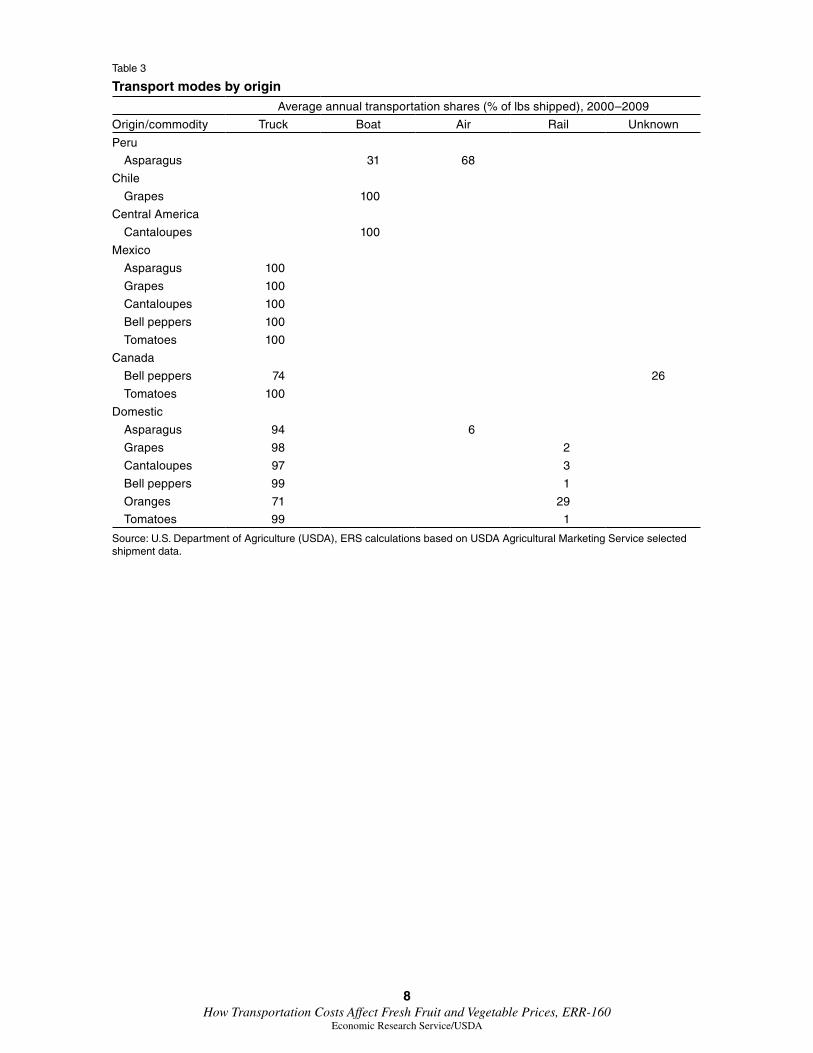
The different import patterns of the produce items determine the typical modes of transport from field to market, likely affecting the sensitivity of the imports to fuel prices. While domestic ship-ments for these commodities are almost exclusively by truck, produce is delivered into the United States via ships, airplanes, or trucks, depending upon the origin. In general, produce items from a specific origin have a common method of transport to the United States border (table 3).3 Growing sources closest to the continental United States tend to use truck transportation, while more distant locations tend to rely on ocean transport or—for commodities like asparagus that are of high value and highly perishable—air transport.

Produce transportation via modes other than trucking is on the rise, concomitant with the strong growth in imports. Imports made up about half the growth in U.S. fruit consumption and a quarter of the growth in vegetable consumption from 1984 to 2004 (Huang and Huang, 2007), and transpor-tation distances have increased proportionately. As Lucier et al. (2006) noted, “Increasingly, fresh fruit imports have been rising during the primary U.S. growing seasons.”

In addition, domestic growing locations have moved across the country to more productive areas. As of 2010, California and Florida accounted for one-half and one-quarter, respectively, of all U.S. fruit acreage. Additionally, California was home to more than 90 percent of all U.S. tree nut acreage. Accordingly, from 1981 to 1998, the average distance for fresh fruits and vegetables to reach the Chicago wholesale terminal market increased by 22 percent, from 1,245 to 1,518 miles (Pirog et al., 2001). Produce shipments have spread beyond the typical North American Free Trade Agreement (NAFTA) trading partners of Canada and Mexico, fresh fruit imports in 2004-06 were primarily (67.9 percent) from South and Central America, Australia, New Zealand, and South Africa. Between 2000 and 2008, NAFTA countries accounted for 69 percent of total U.S. fresh vegetable imports. In both cases, there is significant variation in source locations throughout the calendar year.

Many technological advances over the last 50 years have enabled perishable items to be shipped from previously impractical locations. The advent of containerized transport, and then of mobile refrigerated containers, in the 1950s and 1960s greatly increased the efficiency and viability of ocean transport (Ballenger et al., 1999). Controlled-atmosphere technologies in containers for the transport of perishable fruits and vegetables have become even more sophisticated in recent years. For easily degraded items of high value, such as asparagus and raspberries, air transport has also been used in recent years to ensure quick delivery to distant markets.

3An exception to this is Peruvian asparagus, which transitioned from being mostly transported by boat (85.8 percent) in 1999 to being almost completely shipped by air (93.9 percent) in 2003 and then back to a mixture of ocean and air transport as fuel prices increased from 2004 through 2009 (air transport share was 86.3 percent in 2004 and 57.8 percent in 2008).



Table 3

Transport modes by originAverage annual transportation shares (% of lbs shipped), 2000–2009

Origin/commodity Truck Boat Air Rail Unknown

Peru

Asparagus 31 68

Chile

Grapes 100

Central America

Cantaloupes 100

Mexico

Asparagus 100

Grapes 100

Cantaloupes 100

Bell peppers 100

Tomatoes 100

Canada

Bell peppers 74 26

Tomatoes 100

Domestic

Asparagus 94 6

Grapes 98 2

Cantaloupes 97 3

Bell peppers 99 1

Oranges 71 29

Tomatoes 99 1

Source: U.S. Department of Agriculture (USDA), ERS calculations based on USDA Agricultural Marketing Service selected shipment data.



Wholesale Produce Prices

This report uses wholesale fresh fruit and vegetable prices collected by USDA’s Agricultural Marketing Service (AMS) for wholesale (terminal) market locations throughout the United States. Thirteen markets—Boston, New York City, Philadelphia, Pittsburgh, Baltimore, Columbia (SC), Atlanta, Miami, Detroit, Chicago, St. Louis, San Francisco, and Los Angeles—represent a variety of geographic regions across the country. These terminal markets facilitate large-quantity sales of wholesale fruits and vegetables from importers and domestic shippers to other wholesalers, retail outlets, and the foodservice industry.

Terminal markets have traditionally handled a large portion of the fresh produce trade in the United States, but since the 1950s they have waned as shippers deal directly with retailers. However, these markets are still important distribution channels, handling an estimated 30 percent of national produce flows (by weight). Terminal markets continue to be important in the marketing of imports and in the disposition of residual fresh produce supply and demand (Cook, 2002). For example, even with the decline of the terminal markets over the last 60 years, the New York market still claims to be the largest produce market in the world, reporting 2.7 billion pounds of fresh fruits and vegetables sold annually (as of 2011).

The wholesale produce pricing data used in our study covers January 2000 through December 2009 and includes daily price observations specified as high/low range, with prices at a given market differentiated by product origin and a number of product specification variables. This detail provides a large number of total price observations per commodity, ranging from over 245,000 for asparagus to over 670,000 for oranges. In our analyses, the data are simplified in several ways to produce a more uniform set of prices with fewer outlying price observations. First, we use a median price instead of the provided high/low range, and we convert the sale prices into dollars per pound from dollars per package. We also aggregate the daily data to weekly data, with groupings of price obser-vations dependent on item size and variety. We then exclude all prices in which recorded comments indicate that a portion of the quantity is “unsalable” or for items for which the condition, quality, or appearance is listed as “poor,” “ordinary,” 4 “fair,” or “holdover.” Finally, price observations for organic produce are also dropped from the analyses.5

Figures 4a–4f track wholesale produce prices from 1998 to 2010. As the figures show, wholesale prices typically have strong intrayear fluctuations, mirroring seasonal supply shifts. The prices for a marketing year, in dollars per pound, are generally centered around a given range, with 2008/09 average prices ranging from $0.38 for cantaloupes to $1.93 for asparagus (1.93). Common to all six produce items across the 12-year span is an increasing price trend, beginning in early 2004. While there may be many reasons behind this, it does roughly coincide with an upward shift in oil prices (fig. 1).

In addition to fluctuations in national produce prices, patterns are apparent at the local market level too. Price movements are common across vastly separated markets (e.g., in January for grapes, cantaloupes, and asparagus) in some months and diverge at other times (figs. 5a-f). Raper et al.

4“Ordinary” in this sense is defined by AMS as “having a heavy percentage of defects as compared with “good.”5Organic produce is dropped because price observations of this type are generally not uniformly distributed across

years or markets and not present in large numbers. When analyzed, organic certification exhibits a very large positive and statistically significant effect on prices.



Figure 4

Seasonal price patterns in recent data

4b–Weekly average wholesale grape pricesPounds

0.50

1.00

1.50

2.00

2.50

3.00

2000w12000w11990w12000w11990w12000w11990w1

4e–Weekly average wholesale pepper pricesPounds

0.50

1.00

1.50

2.00

2000w12000w11990w12000w11990w12000w11990w1

4c–Weekly average wholesale asparagus pricesPounds

1.00

2.00

3.00

4.00

2000w12000w11990w12000w11990w12000w11990w1

4f–Weekly average wholesale tomato pricesPounds

0.50

1.00

1.50

2.00

2.50

2000w12000w11990w12000w11990w12000w11990w1

Source: U.S. Department of Agriculture (USDA), Economic Research Service (ERS) calculations based on data from USDA Agricultural Marketing Service.

4d–Weekly average wholesale orange pricesPounds

0.20

0.30

0.40

0.50

0.60

0.70

2000w12000w11990w12000w11990w12000w11990w1

4a–Weekly average wholesale cantaloupe pricesPounds

0.20

0.30

0.40

0.50

0.60

0.70

2000w12000w11990w12000w11990w12000w11990w1



Figure 5

Within-year seasonal price patterns by market

5b–Weekly average wholesale grape prices, 2008/09Dollars/lbs.

1.8

1.6

1.0

1.2

1.4

49 53413733 45252117 29951 13

New YorkChicago Los Angeles

Boston

5e–Weekly average wholesale pepper prices, 2008/09Dollars/lbs.

1.80

1.20

0.80

1.40

1.00

1.60

49 53413733 45252117 29951 13


Boston

5c–Weekly average wholesale asparagus prices, 2008/09Dollars/lbs.

3.0

2.5

1.0

1.5

2.0

49 53413733 45252117 29951 13


Boston

5f–Weekly average wholesale tomato prices, 2008/09Dollars/lbs.

1.60

1.00

0.60

1.20

0.80

1.40

49 53413733 45252117 29951 13


Boston

Source: U.S. Department of Agriculture (USDA), Economic Research Service (ERS) calculations based on data from USDA Agricultural Marketing Service.

5d–Weekly average wholesale orange prices, 2008/09Dollars/lbs.

0.80

0.70

0.30

0.40

0.50

0.60

49 53413733 45252117 29951 13


Boston

5a–Weekly average wholesale cantaloupe prices, 2008/09Dollars/lbs.

0.8

0.6

0.2

0.4

49 53413733 45252117 29951 13


Boston



(2009), in their study of the wholesale peach market, find that a greater variety of local supply origins for markets in the domestic growing season leads to greater differences in prices among markets, while prices across markets vary less during the import season when sources are fewer.

These market-level price movements have a geographic element that becomes more evident in the 2008-09 set of season-average prices (table 4). For produce items grown predominantly in California (asparagus, grapes, cantaloupes, and oranges), prices increase moving west to east in the domestic season. Transportation costs increase with distance, and the increase in wholesale prices as produce items move from west to east calls for further investigation.6 In the import season, this trend does not hold and prices are more similar across the examined markets.

6For asparagus and oranges, this trend is weaker in Chicago than in New York, likely due to the Chicago market hav-ing less California-grown produce.



Table 4

Terminal market commodity origins during the domestic seasonSeasonal marketing statistics (2008/09 averages)

Domestic season offerings shares3

Seasonal average prices1 Domestically produced

Commodity/city DomesticNon-

domestic2 CaliforniaNot

California Import

——————— Percent ———————

Grapes

Los Angeles 1.06 1.18 95.2 0.0 4.8

Chicago 1.12 1.17 87.3 1.1 11.6

New York 1.23 1.28 90.8 1.2 8.0

Boston 1.37 1.38 87.5 1.1 11.4

Asparagus

Los Angeles 1.69 1.91 40.9 11.3 47.7

Chicago 1.92 1.85 6.4 22.5 71.1

New York 1.80 1.85 18.7 30.2 51.1

Boston 1.98 2.06 24.4 10.5 65.2

Cantaloupes

Los Angeles 0.24 0.36 56.5 36.0 7.5

Chicago 0.35 0.34 71.0 23.3 5.6

New York 0.38 0.33 64.7 31.2 4.0

Boston 0.46 0.39 66.8 31.8 1.3

Oranges

Los Angeles 0.42 NA 79.7 11.6 8.7

Chicago 0.52 NA 55.5 34.2 10.3

New York 0.44 NA 62.7 35.5 1.8

Boston 0.54 NA 58.3 32.4 9.3

Peppers

Los Angeles 1.29 NA 32.4 0.0 67.6

Chicago 1.33 NA 15.3 20.8 63.9

New York 1.12 NA 11.5 34.1 54.4

Boston 1.24 NA 4.5 36.3 59.2

Tomatoes

Los Angeles 0.80 NA 21.2 2.8 76.0

Chicago 1.04 NA 8.5 34.1 57.4

New York 0.95 NA 7.9 44.0 48.1

Boston 1.00 NA 3.5 51.1 45.41Dollars per pound; the domestic season is defined as the weekly range where 80 percent of domestic offerings occur. 2For oranges, peppers, and tomatoes, significant domestic production occurs throughout the calendar year, and so for these commodities, numbers are representative of the entire year.3Shares of sale price observations

Source: U.S. Department of Agriculture (USDA), ERS calculations based on USDA Agricultural Marketing Service

selected shipment data.



How Fuel Prices Affect Produce Prices

Our investigation of the ways in which fuel prices affect fresh produce prices involves three steps, each analyzing a sector of relevant data: truck rates, wholesale margins, and prices across multiple origins.

Trucking Rates

A data series of transportation costs from USDA’s Agricultural Marketing Service (AMS) provides detailed weekly rates for full-load produce truck transport between California (specifically, San Joaquin Valley) and a number of U.S. cities for 2005-2009.7 While the data do not cover the trans-portation costs for all routes and items arriving in the wholesale markets, they do provide informa-tion for routes common in fresh produce marketing. In the 2008/09 terminal market price data, the share of total price observations that show California as the origin ranges from a low of 11.3 percent for tomatoes up to 64.5 percent for oranges.

We estimate how rates for routes of varying distances may be affected differently by changing fuel prices.8 AMS calculates the transportation cost, in dollars per pound, from the weekly route price—the median of the listed weekly high/low total cost for the route— under the assumption that a full load is 38,000 pounds.9 Plotting a selection of the route prices, in dollars per pound, illustrates a strong seasonal component, a high correlation of price lows and highs among routes, and a spike in 2008 corresponding closely to the spike in diesel prices (fig. 6).

To look at the relationship of transportation costs with fuel prices more closely, we constructed the following basic regression model and applied it to the different route price series:

( ) ( ) ( ) ( ) ( )21 2 3 4i ,d diesel seas sup k t _ rate ln P trend trend + ’ t _ season ’ t _ supply ,β β β β β β(1) = + + + +

where t_ratei, d is the dollar-per-pound in week i median cost of transport from the San Joaquin Valley to destination city d; t_season is a vector of seasonal dummy variables;10 t_supply is a vector of qualitative supply dummy variables k;11 and Pdiesel is the average of the previous 5 weeks of U.S.

7Fruit and Vegetables Programs, Market News Branch.8Truck transport is commonly cited as the dominant mode of domestic transportation for fresh fruits and vegetables;

94 percent of such transport was by truck in 2002 (Denicoff et al., 2010).9The authors do not feel the assumption of a 38,000-pound load to be significantly strong because, if applied to each

observation, the assumption would affect the magnitudes of the results but not the relationships within the results. Dollars per pound is used here instead of other price measures (i.e., total route cost, dollars per mile) because it enables direct comparisons to produce prices, which are also expressed in dollars per pound.

10The seasonal dummy variables divide the calendar year into quarters. They correspond to January through March, April through June, July through September, and October through December.

11These variables vary slightly by commodity. Using conventions drawn from and assigned by AMS, they describe the quality, appearance, condition, and, when applicable, the size and color of the produce being shipped. The full list of descriptors is available from the authors upon request.



on-highway average diesel prices.12 We also included a linear and quadratic time trend to account for technological growth and other time-specific factors.13

In the results of this regression (table 5), several basic patterns arise relating the transport cost to the distance traveled.14 First, in all routes, save for the short route from San Joaquin Valley to Los Angeles, diesel prices were found to have a statistically significant effect on transport prices. As the distance of the route increased, fuel prices increased the $/lb shipping cost, but the relationship between truck rates and mileage was not linear across all cities.15 For example, the distance traveled from San Joaquin Valley to Dallas is less than half that traveled to Boston, but the average truck rate for the Dallas route is over 60 percent that of the Boston route. Further, the average truck rates for routes to Chicago and Dallas are approximately equal, although the Chicago route is 600 miles longer.

12We tested each time series value for the presence of a unit root using the Augmented Dickey-Fuller test. Unit roots present problems because they indicate that regression results may be spurious. While the inclusion of a time trend typi-cally attenuates concerns in this regard, the truck rate series for Dallas and Los Angeles strongly indicated the presence of unit roots. As a result, we estimate the equations for these cities on first-differenced data.

13We also experimented with a yearly fixed-effects estimation. This approach yielded a number of counterintuitive results, likely stemming from the fact that several of these commodities undergo growing seasons or peak distribution periods that overlap calendar years. Given that it is not clear how to most accurately delineate years on a per commodity basis, any approach in this respect would necessarily be ad hoc.

14Due to the large number of routes in this study and the primary focus on fuel price effects, only coefficients for the fuel price variables will be listed in the results tables. Results for the other variables are available upon request.

15The reason for the nonlinear relationships likely has to do with different demands for the different routes and differ-ing possibilities for back-hauling from the destination cities.

Selected produce truck rates (San Joaquin Valley origin) and diesel prices, 2005–2009$/lbs.

Note: Diesel Price refers to the on-highway U.S. average price; truck rates were converted to dollars per pound using the assumed load of 38,000 pounds.

Source: U.S. Department of Agriculture, Economic Research calculations based on data from USDA Agricultural Marketing Service and U.S. Department of Energy, Energy Information Administration.

Figure 6

2005w1 2008w12007w12006w1 2010w12009w1

$/gallon

0

0.05

0.10

0.15

0.20

0.25

2.00

3.00

4.00

5.00

BostonAtlantaDallas

Diesel PriceNew YorkChicagoLos Angeles



Fuel-price sensitivity, however, generally increases with distance traveled. The relationship holds across nearly all routes. The coefficient on diesel prices is insignificant for the Los Angeles route, and that estimation has very poor explanatory power. The Boston, New York, Miami, and Philadelphia routes are the longest, each closely comparable in length and with statistically identical fuel price coefficients that increase slightly with distance. The coefficient for Atlanta is about 80 percent that for New York, and the route is 80 percent as long. Only Dallas deviates somewhat from this linear relationship, with a coefficient that is one-third New York’s for half the traveling distance.16

The nonlinearity in the relationship between truck rates and mileage suggests an investigation of the importance of diesel costs in determining overall shipping costs. Given that our regression model is estimated with truck rates in $US diesel prices in natural log form, it is possible to calculate the estimated impact that a doubling of diesel prices would have on truck rates. In our case, that would be simply the coefficient on diesel prices divided by the average truck rate, by route. If diesel prices were to double, our results suggest that average truck rates for Boston, New York, Miami, Philadelphia, Atlanta, and Chicago would all increase by 46 to 48 percent. Dallas truck rates would rise about 25 percent, and those for Los Angeles would increase the least, by about 11 percent.17 Overall, this first step of our analysis suggests that fuel prices affect fresh produce prices through transport costs and that there is a logical pattern of increasing marketing costs as the distance from origin to market grows.

16Using the reported standard errors, it is possible to construct 95-percent confidence intervals for the diesel price coef-ficients. The estimated Boston, New York, Philadelphia, Miami, Atlanta, and Chicago coefficients are not statistically different from one another. The Dallas coefficient is statistically smaller than those for Boston, New York, Philadelphia, and Miami.

17Although this effect would not be expected, in practice, given that the coefficient on diesel prices is not significant.

Table 5

Regression results for the truck rate analysis, California-sourced produceBoston New York Miami Philadelphia Atlanta Chicago Dallas Los Angeles

Pdiesel1 0.072*** 0.071*** 0.070*** 0.067*** 0.057*** 0.048*** 0.023* 0.003

(0.007) (0.007) (0.006) (0.007) (0.005) (0.006) (0.011) (0.048)

R2 67.29 65.53 70.20 66.83 69.62 57.98 14.55 0.30

N 239 242 236 242 239 240 232 237

Avg. t_rate 0.154 0.148 0.149 0.145 0.118 0.104 0.091 0.026

Distance 3,151 2,930 2,882 2,856 2,313 2,156 1,572 222% Increase in t_rate 46.75 47.97 46.98 46.21 48.31 46.16 25.27 11.54

(*) denotes significance at least at the 10-percent level, (**) denotes significance at least at the 5-percent level,

(***) denotes significance at least at the 1-percent level.

Robust standard errors for the estimated diesel price coefficients are in parentheses.1For the sake of brevity, the only reported coefficient is for the key variable of interest, Pdiesel. The remaining independent variables included in this model are t_season, t_supply, and linear and quadratic time trends. The full regression results are available from the authors upon request.

“Distance” refers to the approximate distance (in road miles) from San Joaquin, CA to the destination city.

“% Increase in t_rate” is the estimated percentage impact on truck rates that would occur given a doubling of diesel prices. It is calculated as the coefficient on Pdiesel divided by the average market-level truck rate.



Wholesale Price Margin

The second step of the analysis is to examine the price margin between shipping-point prices (a proxy for farm-level prices) and wholesale produce prices. We use price observations for California-grown produce because the shipping-point price data are exclusive of imports and because California is a significant supplier of all six commodities to wholesale terminal markets. Although this limits the scope of the analysis in terms of supply origins, a farm-level price proxy does enable us to distinguish fuel price effects that are more precisely related to transportation costs.

This measure of the margin between wholesale prices and approximate farm prices is constructed from wholesale terminal market prices and free-on-board shipping-point prices for each commodity, provided by AMS. These shipping-point prices are very similar (e.g., daily frequency, item size and variety information, and price specified as high or low range) to the terminal market price data and thus are treated in a similar manner. AMS does not track all shipping-point prices, so the number of price observations over 2000-2009 varies considerably by commodity. In this analysis, the number of observations depends on the significance of California as a supplier of the commodity.

To create a variable for the wholesale margin, we decided to match terminal market prices with shipping-point prices lagged by 1 week, since most markets are likely to be over 2,000 miles from California. In addition, we wanted to avoid the possibility (which could arise in weekly aggregation) of shipping-point prices leading terminal market prices. Item size and variety are used to match prices to obtain a more consistent measure.18 Thus, shipping points of produce items matched to wholesale prices provide approximate differences between farm and wholesale prices that can be tracked over time.

With this estimated measure, we focus on the relationship between fuel prices (specifically, U.S. diesel prices, as the shipments being analyzed are all domestic) and the wholesale margin. To isolate the fuel price impact, we construct a simple regression model with the following form (for each commodity):

( ) ( ) ( )( ) ( ) ( ) ( ) ( )

( ) ( ) ( )

, , , , 1 2 3 4 ,

5 , 6 7 , 8 9

210

– ln ln _ ln _

_ _ _ ln

’ ’

w d j w d j m w w d

w d w w d diesel

spec p seas s

TM SP supply total off city off

share off sp dem share light P trend

trend spec season

β β β β

β β β β β

β β β

(2) = + + +

+ + + + +

+ + + ,

where TMw,d,j (or SPw,d,j) is the terminal market (or shipping point) price for week w, market d, and commodity j (asparagus, tomatoes, etc.); season is a vector of dummy variables to capture seasonality; specp is commodity fixed-effects p (dummy variables for particular varieties and sizes); supplym is the estimated overall monthly U.S. supply of the fresh produce item for month m; total_offw is the total number of weekly observed prices in all markets for items originating from California; city_offw,d is the total weekly number of observed prices at a terminal market; share_offw,d is the share of the week’s prices at a terminal market that are from California; sp_demw is the share of the week’s shipping-point observations where demand was listed as at least “good”; share_lightw,d is the share of the week’s terminal market price observations where the offerings

18For grapes, prices are not matched on size due to the large number of size and variety combinations possible in the markets and the consequent lower number of price matches when both dimensions are used.



were described as “light”; and Pdiesel is the average of the previous 5 weeks’ on-highway average diesel price. 19, 20

As with the regression model (1), we include linear and quadratic time trends. We estimate the diesel price impact for all commodities and cities analyzed (table 6), with model statistics listed in appendix table A1. Recall (from interpreting the coefficients) that a 100-percent increase in Pdiesel will be associated with an increase of the price margin by ββ8 because Pdiesel is in natural log form and the dependent variable is in levels (dollars per pound). The coefficients in table 6 can be directly compared across markets and commodities to gain a sense of expected changes in the wholesale price margin, expressed in dollars per pound.

Fuel prices are a statistically significant factor in determining the difference between domestic wholesale and farm-level produce prices: the large majority of diesel price coefficients are positive and significant (table 6). The estimated magnitudes vary considerably by commodity and terminal market,21 but a 100-percent increase in the price of diesel fuel can be expected to increase the produce marketing margins from between 3 to 19 cents per pound.

By region, the regression results generally show a pattern of increasing sensitivity to fuel prices with distance, with the diesel coefficients for the Northeast and Southeast markets generally larger than those for the Midwest, which are in turn larger in most cases than those for California (table 6). This is most clear when examining the population-weighted average coefficients by region and commodity. For asparagus, the average coefficient for California is higher than that for the Midwest, but for the most part, marketing margins are more sensitive to fuel prices with distance.

Examining the coefficient of variation (CV) across commodities but within markets helps clarify the extent to which the impact of fuel prices varies.22 The CV for the average regional coefficients is highest in California at 1.5 and decreases with distance, reaching a minimum of 0.5 for the Northeast markets. This suggests that transportation costs may serve to mitigate wholesale price volatility across commodities and possibly within commodity markets across time. As the fuel share of wholesale prices increases, the potential for volatility deriving from alternative supply-side sources, such as labor or financing costs, decreases.

It is interesting to note how the fuel price effect varies with mileage and how this variation differs across commodities. For example, the effect for asparagus—an item for which the California

19This monthly aggregate supply variable estimates a basic accounting of the total U.S. supply for a given fresh pro-duce item by combining monthly import and export data from the USDA Foreign Agricultural Service (FAS) with annual U.S. production data from the USDA-ERS’s Food Availability Data System, which has been has been scaled to monthly numbers using domestic movement data from AMS.

20Many empirical approaches to studying marketing margins have employed structural models, examining supply and demand simultaneously in order to identify key economic relationships (Wohlgenant, 2001). Our markets of interest benefit from highly inelastic supply in the short term, but nevertheless, in this reduced-form setting the shifters for sea-sonality must be thought of as proxies for changes in demand. In practice, a wide number of factors other than price can influence demand.

21The markets are generally categorized by region in a geographic manner, with assignments as follows: Califor-nia—Los Angeles and San Francisco; Midwest—Detroit, Chicago, and St. Louis; Southeast—Atlanta, Columbia, and Baltimore; Northeast—Boston, New York, Philadelphia, and Pittsburgh. Geographically, Baltimore may fit more closely in the Northeast, but the results for this market are much closer to the Atlanta market in both produce price analyses.

22The CV is the sample standard deviation of a variable divided by the sample mean. It is a unitless measure of disper-sion that can be interpreted as a percentage and is ideal for comparing dispersion across samples with different units or means.



marketing season is relatively short and for which there is a continuous, significant supply of imports—differs fundamentally from that for cantaloupes and oranges. Estimates of the fuel price effects for asparagus are generally much higher than for the other commodities, and there is no clear pattern across geographic markets of their magnitudes. However, California is the dominant supplier to all terminal markets for much of the year for cantaloupes and oranges. For these two items, there is a well-defined pattern of increasing sensitivity to fuel prices as the distance from California increases, and within a given market, the coefficients are very similar for both cantaloupes and oranges.

For the three lowest priced produce items (cantaloupes, oranges, and tomatoes), the average whole-sale price margins themselves (appendix table A1) follow a logical pattern of increasing west to east, indicating that transport costs are a particularly significant factor in determining wholesale prices. Peppers also follow this pattern to some extent, while asparagus and grapes, which both have notice-ably higher average margins in our data, have similar margins across markets. A comparison of the diesel price coefficients with the results in the appendix suggests that, in general, a large portion of the wholesale margin is related to fuel costs for transport, given that both sensitivity to fuel prices and the margins themselves increase with distance for four of the six commodities.

Table 6

Regression results for the diesel price coefficient, ln(Pdiesel), in the wholesale price margin analysis

Asparagus Grapes Cantaloupes Oranges Tomatoes PeppersCoefficient of

Variation1

NortheastBoston 0.111*** 0.187*** 0.089*** 0.075*** 0.115*** 0.116*** 0.361

New York 0.175*** 0.051*** 0.066*** 0.061*** 0.048*** -0.003 0.885

Philadelphia 0.094*** 0.099*** 0.076*** 0.085*** 0.073*** -0.011 0.586

Pittsburgh 0.048 0.131*** 0.055*** 0.091*** 0.047*** 0.048*** 0.490

Average2 0.141 0.085 0.070 0.070 0.062 0.016 0.544

SoutheastAtlanta 0.333*** 0.106*** 0.079*** 0.102*** 0.137*** 0.051*** 0.752

Columbia N/A 0.026 0.075*** 0.082*** 0.067*** -0.224*** 24.992

Baltimore 0.169*** 0.156*** 0.092*** 0.110*** 0.056*** 0.090*** 0.383

Average 0.253 0.114 0.083 0.103 0.106 0.039 0.621

MidwestDetroit 0.041 0.121*** 0.076*** 0.032*** 0.050*** 0.036*** 0.574

Chicago 0.023 0.070*** 0.032*** 0.044*** -0.039*** 0.060*** 1.223

St. Louis -0.046 0.162*** 0.058*** 0.059*** 0.064*** 0.060*** 1.106

Average 0.016 0.099 0.048 0.043 0.002 0.054 0.775

CaliforniaLos Angeles 0.124*** -0.022 -0.002 0.029*** 0.000 0.052*** 1.751

San Francisco 0.160*** 0.105*** 0.018*** 0.006** -0.029*** 0.050*** 1.350

Average 0.133 0.010 0.003 0.023 -0.007 0.051 1.458 (*) denotes significance at least at the 10-percent level, (**) denotes significance at least at the 5-percent level, (***) denotes significance at

least at the 1-percent level.1The coefficient of variation is a measure of volatility that is calculated as the standard deviation of the estimated regression coefficients, across commodities but within markets, divided by their mean.2The average coefficients, by region, are weighted by population as provided by the 2010 Census.

“NA” signifies that this model was not used due to a small sample size.

The wholesale price margin analysis features a number of independent variables not reported in the table. These are season, supply, total_off, city_off, share_off, sp_dem, share_light, and linear and quadratic time trends. The complete regression results are available from the authors upon request.



Prices From Multiple Origins

As the last step in analyzing the relationship between fuel prices and wholesale price margins, we look at data on produce shipments from multiple sources. In these estimates, we omit a farm-price measure due to data limitations. The objective is to explore the impact of fuel costs on fresh produce prices by focusing on the entire calendar year and a more varied set of transport routes.

We construct a model very similar to the wholesale-price-margin model (2) in the previous section, one that can be applied to a greater variety of shipping routes. These routes are again organized by market and origin and commodity, using the major origins shown in figures 2a-f along with a few others that are significant in a limited number of markets.23 Our wholesale price model is:

( ) ( ) ( )( ) ( ) ( ) ( )

( ) ( ) ( )

w d j o m p p w o

w d p o 5 w d o p w d oil

seas s

TM supply spec total off

city off + share off share light P

trend trend season

, , , 1 2 3, 3 ,

4 , , , , , , 6 , 7

29 10

ln ln _

ln _ _ _ ln

’ ,

β β β β

β β β β

β β β

(3) = + + +

+ + +

+ + +

where the representations other than those given for model (2) are TMw,d,j,o for the terminal market price for week w, market d, commodity j, and origin o; total_offw,o as the total number of weekly observed prices in all markets from origin o; city_offw,d,p,o as the total weekly number of observed prices of specification p from origin o at a terminal market; share_offw,d,p,o as the share of the week’s prices at a terminal market that were from origin o; and Poil for the average of the previous 5 weeks’ world crude oil spot price.24

The supply origins in these markets can vary both by commodity and geographic location of the market (table 4). With commodities such as grapes and cantaloupes, there is a specific domestic origins-only season with a single region (California, for both items) accounting for the vast majority of price observations in the markets, complemented by an off-season when a single exporting region supplies most terminal markets. This implies that for these two cases, at most points in the year, there are only a few supply routes per market at a given time.25 This is in contrast to tomatoes and bell peppers, where for most of the year there are several different supply regions producing concur-rently. For these two commodities, production sourcing is less concentrated, and the produce sold at a given time in the terminal markets covers a vast array of transport distances. For example, data for the New York City market in the summer months include a significant number of price observations for tomatoes from California, Mexico, Canada, and regional sources, all occurring concurrently. When multiple origins supply an identical (or nearly so) commodity to a given market, arbitrage within terminal markets may limit the capacity for agents to adjust produce prices quickly and completely in light of fuel price fluctuations. This possibility should be kept in mind when inter-preting the results.

23The routes are organized by origin in this analysis because of both the clear need to account for origin-specific fixed effects and fuel price coefficients and for the greater flexibility of allowing the season and supply variables to vary significantly based on the origin.

24This more general fuel price is used here rather than a diesel price (even though diesel is a common fuel in truck and ocean transport) because of the greater variety of origins (and thus different fuel types) represented in this analysis.

25Oranges also fit closely with this last statement, since imports generally make up a small share of offerings in all markets and domestic supply is primarily from Florida or California, with offerings from Florida tending to show up more in East Coast markets.



Applying our wholesale price model to the different commodities, markets, and origins recon-firms the statistical significance of fuel prices in determining wholesale fresh produce prices and suggests a number of underlying patterns. Correlation coefficients with Poil —the average of the previous 5 weeks’ world crude oil spot price from model (3)—are listed in table 7 for each commodity, market, and origin series (with sample statistics listed in appendix table A2). There is a general similarity among coefficient magnitudes within regions and by origin that, along with the statistical significance of the estimates, implies that fuel prices are an important determinant of wholesale fresh produce prices and that the fuel price effect is geographically different.26 The overarching theme of the results remains that the impact of variations in the fuel price increases with distance to market; however, with more complicated routes and more origins for comparison purposes, there are caveats to this statement. The six commodities analyzed lend themselves to a convenient organization for discussion due to differences in their sourcing and the patterns observed in their fuel price coefficients.

Cantaloupes and Oranges

Cantaloupes come largely from California and Central America, enabling a clear comparison of fuel price effects on domestic and imported wholesale prices. The coefficients corresponding to California as the product origin correlate with distance from the origin, as they did in the wholesale price margin analysis. However, the same relationship does not apply to cantaloupes from Central America,27 which show very little sensitivity to changes in fuel prices.

A comparison with the California origin (table 6) for cantaloupes shows lower coefficients for Central America, even when the marketing distance is much longer. Although many factors may be contributing to this difference in impacts, a few immediately stand out. Foremost is the method of transportation. Cantaloupes are trucked across the United States, but all tracked shipments from Central America arrived by ship, and ocean transport is only about 10 percent as energy-intensive as truck transport. The dispersion in coefficients could also be due to each of these originators being dominant suppliers when they appear in the markets, with their time periods typically distinct within the calendar year.

The results for oranges exhibit, similar to cantaloupes, an increasing fuel price effect with distance. Throughout each season of the year, California and Florida account for the most and second-most price observations for oranges, respectively, while imports constitute only a small share of U.S. orange supplies. In the case of California-grown oranges, the familiar pattern emerges of lower fuel price sensitivity in the California markets and higher coefficients as distance increases from the San Joaquin Valley.

For Florida-grown oranges, the story is somewhat different. The fuel price coefficients are lowest for the Miami market, but in the other regions there is less distinction based on geography. Notably, the estimated fuel price sensitivity in the Northeast markets is the highest (table 7), even though the Midwest and California markets are geographically more distant. Thus, with oranges and cantaloupes, we are able to identify an increasing influence of fuel prices on wholesale prices for commodities that have a relatively small number of geographic sources and that exhibit a clear, year-long hierarchy of total supply to U.S. consumers.

26There are also a few cases where some dispersion exists with a region and origin group; possible causes for some of these instances will be discussed later.

27Central America in this study refers to the countries of Costa Rica, Guatemala, and Honduras.



Table 7

Regression results for oil price coefficient, ln (Poil ), in the multiple origin price analysisAsparagus Cantaloupes Peppers

California Mexico Peru CaliforniaCentral America California Florida Mexico Canada

Northeast

Boston 0.350*** 0.373*** 0.225*** 0.085*** 0.031*** 0.251*** 0.166*** 0.333*** 0.207***

New York 0.565*** 0.225*** 0.220*** 0.047*** -0.013* 0.159*** 0.147*** 0.324*** 0.288***

Philadelphia 0.380*** 0.367*** 0.248*** 0.066*** 0.028*** 0.142** 0.111*** 0.391*** 0.356***

Pittsburgh 0.446*** 0.303*** 0.351*** 0.058*** 0.028*** 0.186*** 0.157*** 0.355*** 0.171***

Average 0.491 0.297 0.236 0.057 0.004 0.171 0.144 0.340 0.280

Florida

Miami 0.634*** 0.261*** 0.330*** 0.080*** 0.021*** 0.063 -0.080*** 0.420*** 0.086

Southeast

Atlanta 0.398*** 0.357*** 0.401*** 0.093*** 0.052*** 0.148*** 0.148*** 0.407*** 0.205***

Columbia 0.161 0.200*** 0.247*** 0.097*** 0.023*** -0.012 0.206*** 0.168*** 0.292***

Baltimore 0.316*** 0.238*** 0.162*** 0.087*** 0.042*** 0.254*** 0.129*** 0.288*** 0.281***

Average 0.352 0.306 0.313 0.091 0.046 0.167 0.147 0.349 0.236

Midwest

Detroit 0.293*** 0.373*** 0.257*** 0.063*** 0.023*** 0.149*** 0.129*** 0.171*** 0.129***

Chicago 0.318*** 0.241*** 0.214*** 0.038*** 0.005 0.177*** 0.100*** 0.045** 0.121***

St. Louis 0.240*** 0.139*** 0.250*** 0.066*** 0.027*** 0.115*** 0.181*** 0.057*** 0.152***

Average 0.298 0.258 0.231 0.049 0.013 0.159 0.121 0.080 0.128

California

Los Angeles 0.341*** 0.363*** 0.187*** 0.005 -0.009 0.131*** N/A 0.132*** N/A

San Francisco 0.434*** 0.226*** 0.269*** 0.035*** 0.021*** 0.212*** N/A 0.170*** 0.466***

Average 0.364 0.328 0.208 0.013 -0.001 0.151 N/A 0.142 0.466

Grapes Oranges Tomatoes

California Chile Mexico California Florida California Florida Mexico

Northeast

Boston 0.299*** 0.268*** 0.147*** 0.102*** 0.096*** 0.242*** 0.255*** 0.041*

New York 0.231*** 0.226*** 0.206*** 0.098*** 0.072*** 0.126*** 0.142*** 0.075***

Philadelphia 0.194*** 0.184*** 0.309*** 0.112*** 0.094*** 0.172*** 0.130*** 0.190***

Pittsburgh 0.299*** 0.227*** 0.176*** 0.125*** 0.107*** 0.130*** 0.161*** 0.102***

Average 0.239 0.224 0.215 0.103 0.082 0.152 0.157 0.094

Florida

Miami 0.232*** 0.099*** 0.172*** 0.110*** 0.025*** 0.099*** 0.054*** 0.174***

Southeast

Atlanta 0.242*** 0.318*** 0.156*** 0.128*** 0.060*** 0.215*** 0.181*** 0.276***

Columbia 0.150*** 0.141*** 0.011 0.118*** 0.059*** 0.221*** 0.224*** 0.330***

Baltimore 0.254*** 0.275*** 0.280*** 0.136*** 0.090*** 0.177*** 0.174*** 0.082***

Average 0.238 0.289 0.182 0.130 0.069 0.204 0.183 0.221

—continued



Tomatoes and Bell Peppers

In table 7, an alternative sourcing picture occurs with tomatoes and bell peppers. Both commodities exhibit supply patterns in which the terminal markets alternate sources throughout the year, princi-pally in seasons with supplies from Mexico/Florida and California/Canada, along with some smaller regional suppliers in the summer months. The patterns for items originating from California and Florida follow a correlation with distance, where markets closest to the production origin show the least fuel price impact. However, as with oranges, for bell peppers and tomatoes from California and Florida the coefficients within the Midwest and Northeast regions are very similar. In looking at the import series, Mexican-sourced items generally have the highest fuel-market price coefficients in those regions, while the Canadian-origin series show the lowest oil price sensitivity in the Midwest, where markets are closest to the growing regions of central and western Canada (in the case of peppers).

Grapes and Asparagus

The last two commodities analyzed, grapes and asparagus, generally have the least recognizable patterns in fuel price coefficients, but oil prices are still a significant determinant in their whole-sale prices. For both commodities, California is the dominant domestic supplier to the terminal markets; however, for asparagus in recent years, the domestic production season has included heavy imports. As noted in the wholesale price margin analysis, this may be an underlying cause for a lack of geographic correlation with the coefficients across markets for asparagus. Imports during the domestic growing season are a further confounding factor in identifying the role of fuel prices, resulting in scattered observed effects.

For grapes (table 7), relatively stronger patterns emerge from the analysis, with coefficient magni-tudes typically similar across origins (especially for California and Chile), and with the lowest values presenting some interesting relationships. California-grown grapes generally show increasing fuel price sensitivity with distance from California, though the pattern is not as clear as it has been for other commodity/origin pairings given that the average commodities for the Northeast, Southeast, and Midwest are all closely comparable. Chilean-grown grapes also have their lowest coefficients for the

Table 7

Regression results for oil price coefficient, ln (Poil ), in the multiple origin price analysis—ContinuedGrapes Oranges Tomatoes

California Chile Mexico California Florida California Florida Mexico

Midwest

Detroit 0.230*** 0.277*** 0.325*** 0.064*** 0.061*** 0.123*** 0.188*** 0.102***

Chicago 0.205*** 0.201*** 0.245*** 0.069*** 0.063*** -0.076*** 0.083*** -0.012

St. Louis 0.293*** 0.307*** 0.325*** 0.088*** 0.082*** 0.162*** 0.241*** 0.164***

Average 0.226 0.239 0.279 0.071 0.066 0.016 0.137 0.047

California

Los Angeles 0.095*** 0.270*** 0.116*** 0.053*** 0.036*** 0.042*** 0.140*** 0.171***

San Francisco 0.211*** 0.272*** 0.266*** 0.052*** 0.026*** 0.078*** 0.111*** 0.134***

Average 0.124 0.271 0.154 0.053 0.033 0.051 0.133 0.162

(*) denotes significance at least at the 10-percent level, (**) denotes significance at least at the 5-percent level, (***) denotes significance at least at the 1-percent level.

“NA” signifies that this model was not used due to a small sample size.

The multiple origins analysis features a number of independent variables not reported in the table. These are season, supply, total_off, city_off, share_off, spec, share_light, and linear and quadratic time trends. The complete regression results are available from the authors upon request.



Northeast, which has the main ports of entry (New York and Philadelphia) for this commodity and origin,28 and for Florida, which has the geographically closest U.S. city (Miami).

There is increasing interest in the economic impacts and viability of local and regional food systems in the United States (Martinez et al., 2010). Economists, policymakers, and agents within U.S. agri-business are interested in the potential impacts of the expansion of local and regional production on food prices and the environment. The difference in the means by which fuel prices influence regional versus national food systems is likely to be an important component in the discussion. The results for the six commodities studied here suggest that there are likely to be important differences in this regard throughout U.S. food supply systems and that the continued growth of imports may have an impact in mitigating regional price volatility that is due to fuel price fluctuations.

Wholesale Price Responses to Oil Price Increases

Our discussion to this point has focused on comparing the values of the oil price coefficients themselves across origins and markets, with the reasoning that this provides a direct and abso-lute measure to compare how oil price changes affect market prices of goods traveling routes of varying lengths. However, it is also worthwhile to gauge how significant these different coef-ficients are relative to the typical produce price for these markets and origins. To facilitate such comparisons, we divide each estimated coefficient on oil prices by the average wholesale market price for the commodity of interest. We then average these ratios, weighting by population, within regions (table 8). Given that we measure the fuel-price sensitivity using the natural log of oil prices, this ratio can be interpreted by the percentage increase in market prices that would be expected given a doubling of oil prices.

Examining these ratios across commodities and regions, we are able to garner new insights into the importance of fuel prices in shaping fresh produce prices. Central American cantaloupe prices again had the least overall sensitivity to oil price changes, showing the potential to increase by only 3 percent given a doubling of oil prices. In most cases, imported commodities show the least sensi-tivity to oil prices for their respective commodities, likely due to the fact that international transport is generally less energy-intensive. On average, for most domestic origins, the results suggest that market prices could be expected to increase by approximately 20 to 28 percent if oil prices doubled. Given the number of commodities with multiple origins and large import shares, however, these are likely to be short-term impacts in many cases. When applicable and all else held constant, import shares can be expected to increase given a sharp rise in domestic produce prices.

These percentages corroborate previous work conducted on fuel and energy impacts on food prices. Canning (2011) calculated the value added of the energy and transportation industries on the retail food dollar to be approximately 10.2 cents. This can be interpreted to mean that a 100-percent increase in fuel and transportation costs would result in an upper-bound 10-percent increase in consumers’ food expenditures (the type of food costs that Canning estimated in his food dollar analysis).29 Given that the figures calculated in table 8 pertain to wholesale prices, which incor-porate fewer labor, packaging, and trade costs, it is expected that the relative impact of fuel prices calculated for wholesale prices should be somewhat higher than the retail price value added.

28Summary of AMS Movement Reports, 2000 through 2009. Available online at http://www.marketnews.usda.gov/portal/fv.

29This is assuming no factor substitution in production.



At the outset of this report, we noted that understanding how fuel prices can affect the levels and volatility of fruit and vegetable prices can affect consumer expenditure patterns. There is timely motivation for research into this relationship, given the importance of fruits and vegetables to consumers’ diets and the breadth of work within USDA and beyond aimed at understanding and promoting American’s consumption of fresh produce. Andreyeva et al. (2010) reviewed the empirical work on this subject to calculate demand elasticities for fruits and vegetables. Twenty studies of fruit demand yielded estimates ranging from 0.16 to 3.02, with an average of 0.70. For vegetables, another 20 studies demonstrated a demand elasticity range of 0.21 to 1.11, with a mean of 0.58. Therefore, fruit and vegetable demand is responsive to price and may well be price elastic for several indi-vidual commodities. Quantifying the potential impacts of fuel price surges on demand, even in the short term, is beyond the scope of this study. Such an analysis would require the estimated impact of fuel price increases on retail produce prices as well as cross-price elasticities among the produce commodities, which are likely to exhibit variation in their fuel-price responsiveness. However, the

Table 8

Comparison of oil price coefficients to average market prices in the multiple origin price analysis1

Northeast Florida Southeast Midwest California Average

Asparagus

California 34.0 41.1 21.8 20.5 22.6 27.9

Mexico 16.9 13.1 17.3 15.1 18.1 16.5

Peru 12.3 17.0 15.2 11.4 9.3 12.1

Cantaloupes

California 19.0 24.2 28.7 17.4 5.6 17.2

Central America 1.2 6.3 14.0 3.9 -0.7 3.1

Peppers

California 19.2 8.1 19.1 20.9 21.0 19.2

Florida 30.7 -14.7 20.0 20.5 N/A 22.5

Mexico 28.2 37.3 27.5 7.1 14.2 21.4

Canada 25.6 N/A 13.0 8.7 24.0 20.0

Grapes

California 22.4 23.2 23.9 21.3 11.8 20.1

Chile 20.8 9.2 28.8 21.0 25.0 21.8

Mexico 19.8 14.8 17.4 25.0 14.3 19.1

Oranges

California 23.8 24.4 29.5 16.1 15.5 21.1

Florida 26.9 9.5 24.0 21.4 N/A 23.5

Tomatoes

California 23.5 14.6 29.0 2.9 8.4 16.0

Florida 22.6 10.3 26.9 21.3 26.6 22.8

Mexico 11.1 21.2 26.6 6.1 22.7 15.0

Note: These numbers represent the multiple origin price analysis oil price coefficient divided by the average market price in the analysis data (scaled up by 100 percent) and then averaged by region. They provide an estimate of how large the oil price coefficients are relative to the overall market prices. They can also be interpreted as the percentage increase in the average market price that would be expected, given a doubling of the fuel price.1The impacts on demand are drawn from estimates of demand elasticities for fruits and vegetables, as reviewed by Andreyeva et al. (2010). Any errors are our own. Each reported value gives the absolute value of the estimated impact on demand, given a doubling of fuel prices, in percentage terms. These calculations assume the complete and symmetrical transmission of wholesale price changes to retail prices.



potential relationship between fresh produce consumption and fuel price increases warrants further investigation, in light of the estimated impacts of fuel price surges on wholesale prices.

Examining the impact of a doubling of fuel prices on wholesale commodity prices shows that the magnitudes of the fuel price coefficients do not necessarily tell the complete story. For example, California grapes have higher oil price coefficients compared with most other commodities, yet their average market prices are also much higher, leading to the overall impact on the wholesale produce price to be relatively low. This is also true for asparagus, with its much higher market price than that for other commodities. Finally, it is not clear whether produce of domestic or international origins have lower average effects of fuel prices on market prices overall. The fuel price share of commodity prices is largely dependent on the region considered, with proximity to growing source and port of entry of key importance.



Conclusions

This study provides empirical insights into how the sensitivity of wholesale prices for fresh produce to transportation costs is related to supply patterns of the produce. Our estimates of this price sensi-tivity are based on analyses of three aspects of produce marketing. The analysis of produce truck transportation rates directly estimates the link between fuel and transport costs across the Nation. The wholesale price margin analysis examines the relationship between fuel costs and terminal market prices, allowing for changes occurring at the farm level within and across years. Finally, the multiple origin analysis gives a comparative picture of the effect on prices from major supply origins across the calendar year and shows patterns that are specific to different sources, which can vary considerably across commodities.

The procedures for our exploration follow general strategies in the existing literature of wholesale produce market pricing models, but these strategies have limitations to be addressed.30 The present study consistently finds unidirectional price influence between the two empirical price measures of fuel and wholesale market prices, but as all of the terminal markets themselves are unique, much is still unknown about local price setting. In addition, certain variables that could provide more preci-sion in the estimation of the pricing models are not available. These variables include exact quanti-ties supplied or total sales to better gauge the supply and demand interaction, as well as upstream produce prices (in the case of the multiple origin analysis) or transport costs to measure the exact margin for all cases. Finally, we looked closely at only six commodities. Although our results may be applicable to other fruits and vegetables with similar supply patterns and pricing characteristics, there is potentially much that is not known about items with different supply characteristics, for example, fruits and vegetables with greater capacity for storage.

Several questions are inherent in our analyses. First, Do large increases in fuel prices foretell significant increases in wholesale fresh produce prices? The answer suggested by the study is yes, supported by the consistency of the price-changing effect across geographic regions, specific to the supply patterns of each commodity. This is illustrated by a comparison of the results for asparagus and cantaloupes or oranges. For high-priced (dollars per pound) produce items such as asparagus, with more mixed transport modes and without clearly defined seasons for different origins, an increase in fuel prices does lead to statistically significant increases in market prices, but effects on particular regions or times of the year are not clearly defined. In contrast, low-priced produce items like cantaloupes or oranges, with more defined supply seasons and basic transport routes, have defi-nite impacts from fuel price changes. During the domestic growing season, fuel price impacts (an increase in wholesale prices) show a strong correlation with distance from the production origin. For imports from a relatively close source (Central America), wholesale price sensitivity to fuel costs was generally found to be minimal. With cantaloupes, the fuel price effect has a clear relationship with time of year because the supply origins are linked to the domestic growing season.

Next, Are wholesale fresh produce price changes from fuel price effects likely to be a strong determinant of market prices? Again, the answer suggested by the study is, yes, in most cases. Aside from Central American cantaloupes, imports were estimated to exhibit an overall average impact of a 12- to 21-percent increase in market prices from a doubling in world oil prices. Domestic prices were also found to have a significant connection to fuel prices, with an overall average impact

30See, for example, Goodwin et al. (1988). Additionally, Wohlgenant (2001) provides a review of the literature up to that date on the economic analysis of marketing margins.



of a 16- to 28-percent increase in market prices from a 100-percent increase in world oil prices. For the domestic cases, there was considerable mitigation in sensitivity if the produce originated in the same State (or, in most cases, adjoining States) where it was marketed.

Further research to extend this analysis to retail prices would be particularly worthwhile. An empir-ical understanding of the relationship between wholesale price volatility and retail price volatility would be valuable, particularly in the context of how these phenomena may differ according to the impact of fuel prices. Our findings also suggest a potential relationship between the length of ship-ping routes and price volatility, which warrants further investigation due to the potential implications for consumer demand and retail price forecasting. Overall, a better understanding of the impact of fuel prices on consumer food expenditures and consumption can add to the body of research on Americans’ adherence to healthy eating guidelines.



References

Andreyeva, T., M. Long, and K. Brownell. 2010. “The Impact of Food Prices on Consumption: A Systematic Review of the Research on the Price Elasticity of the Demand for Food,” American Journal of Public Health 100(2):216-22.

Ballenger, N., W. Coyle, W. Hall, B. McGregor, and R. Hawkins. 1999. “Transportation Technology Eases the Journey for Perishables Going Abroad,” Agricultural Outlook. U.S. Department of Agriculture, Economic Research Service.

Calvin, L., and R. Cook. 2001. U.S. Fresh Fruit and Vegetable Marketing: Emerging Trade Practices, Trends, and Issues. Agricultural Economic Report 795, U.S. Department of Agriculture, Economic Research Service.

Canning, P. 2011. A Revised and Expanded Food Dollar Series: A Better Understanding of Our Food Costs. Economic Research Report 114., U.S. Department of Agriculture, Economic Research Service.

Cook, R. 2002. “The Dynamic U.S. Fresh Produce Industry: An Industry in Transition.” Chapter in A. Kader (ed.), Postharvest Technology of Horticultural Crops, Third Edition. University of California at Davis, Division of Agriculture and Natural Resources, Publication 3311.

Denicoff, M., E. Jessup, A. Taylor, and D. Nibarger. 2010. “The Importance of Freight Transportation to Agriculture.” Chapter in Study of Rural Transportation Issues, Congressionally mandated study produced by the U.S. Department of Agriculture and the U.S. Department of Transportation.

Gilbert, C. 2010. “How to Understand High Food Prices,” Journal of Agricultural Economics 61(2):398-425.

Goodwin, H., S. Fuller, O. Capps, and O. Asgill. 1988. “Factors Affecting Fresh Potato Price in Selected Terminal Markets,” Western Journal of Agricultural Economics 13(2):233-43.

Hendrickson, J. 1994. Energy Use in the U.S. Food System: a Summary of Existing Research and Analysis. Center for Integrated Agricultural Systems, University of Wisconsin-Madison, Madison, WI.

Huang, S., and K. Huang. 2007. Increased U.S. Imports of Fresh Fruit and Vegetables. Outlook FTS 328-01, U.S. Department of Agriculture, Economic Research Service.

Lucier, G., S. Pollack, M. Ali, and A. Perez. 2006. Fruit and Vegetable Backgrounder. Outlook VGS 313-01, U.S. Department of Agriculture, Economic Research Service.

Martinez, S., M. Hand, M. Da Pra, S. Pollock, K. Ralston, T. Smith, S. Vogel, S. Clark, L. Lohr, S. Low, and C. Newman. 2010. Local Food Systems: Concepts, Impacts, and Issues. Economic Research Report 97. U.S. Department of Agriculture, Economic Research Service.



Pirog, R., T. Van Pelt, K. Enshayan, and E. Cook. 2001. Food Fuel, and Freeways: An Iowa Perspective on How Far Food Travels, Fuel Usage, and Greenhouse Gas Emissions. Leopold Center for Sustainable Agriculture, Ames, IA.

Pollack, S. 2001. “Consumer Demand for Fruit and Vegetables: The U.S. Example.” Chapter in A. Regmi (ed.), Changing Structure of Global Food Consumption and Trade. Agriculture and Trade Report WRS 01-1. U.S. Department of Agriculture, Economic Research Service.

Raper, K., S. Thornsbury, and C. Aguilar. 2009. “Regional Wholesale Price Relationships in the Presence of Counter-Seasonal Imports,” Journal of Agricultural and Applied Economics 41(1):271-90.

Sands, R., P. Westcott, M. Price, J. Beckman, E. Leibtag, G. Lucier, W. McBride, D. McGranahan, M. Morehart, E. Roeger, G. Schaible, and T. Wojan. 2011. Impacts of Higher Energy Prices on Agriculture and Rural Economies. Economic Research Report 123, U.S. Department of Agriculture, Economic Research Service, Washington, DC.

Tegene, A. 2009. “High and Volatile Commodity Prices: What Do They Mean for Food Prices and Consumers: Discussion,” American Journal of Agricultural Economics 91(5):1468-69.

U.S. Department of Agriculture, Agricultural Marketing Service. 2009. Agricultural Refrigerated Truck Quarterly. RTQ-4th Quarter. U.S. Department of Agriculture, Washington, DC.

Weber, C., and H. Matthews. 2008. “Food-Miles and the Relative Climate Impacts of Food Choices in the United States,” Environmental Science and Technology 42(10):3508-13.

Wendt, M., and J. Todd. 2011. The Effect of Food and Beverage Prices on Children’s Weights. Economic Research Report 118. U.S. Department of Agriculture, Economic Research Service, Washington, DC.

Wohlgenant, M. 2001. “Marketing Margins: Empirical Analysis.” Chapter in B. Gardner and G. Rausser (eds.), Handbook of Agricultural Economics, Elsevier Science.



Appendix: Regression model sample statistics for wholesale price analyses

Table A1

Average margins and sample statistics for the wholesale price margin analysisAsparagus Grapes Cantaloupes

Market E(Y)1 Obs. R2 E(Y) Obs. R2 E(Y) Obs. R2

Boston 0.28 356 0.23 0.29 1,192 0.36 0.15 696 0.61

New York 0.24 299 0.32 0.31 1,176 0.23 0.15 697 0.46

Philadelphia 0.21 271 0.29 0.24 1,196 0.20 0.14 704 0.57

Pittsburgh 0.33 306 0.23 0.24 992 0.34 0.14 664 0.44

Atlanta 0.53 177 0.40 0.25 931 0.23 0.15 723 0.58

Columbia NA NA NA 0.36 682 0.26 0.20 438 0.50

Baltimore 0.31 321 0.37 0.28 1,054 0.38 0.17 727 0.57

Detroit 0.28 284 0.37 0.30 1,207 0.28 0.15 668 0.50

Chicago 0.28 274 0.20 0.28 939 0.11 0.13 757 0.23

St. Louis 0.25 196 0.31 0.27 832 0.31 0.11 634 0.45

Los Angeles 0.26 410 0.36 0.24 1,006 0.17 0.05 628 0.43

San Francisco 0.25 401 0.35 0.29 1,164 0.25 0.07 679 0.33

Oranges Tomatoes Peppers

Market E(Y)1 Obs. R2 E(Y) Obs. R2 E(Y) Obs. R2

Boston 0.18 3,798 0.45 0.26 371 0.35 0.17 332 0.17

New York 0.16 3,510 0.32 0.22 473 0.40 0.16 537 0.23

Philadelphia 0.17 3,305 0.36 0.22 368 0.31 0.16 522 0.15

Pittsburgh 0.20 3,205 0.67 0.23 449 0.39 0.18 475 0.37

Atlanta 0.17 2,772 0.51 0.22 480 0.43 0.18 498 0.21

Columbia 0.17 1,654 0.69 0.21 290 0.16 NA NA NA

Baltimore 0.17 3,604 0.54 0.28 329 0.34 0.22 531 0.38

Detroit 0.17 3,527 0.24 0.17 1,054 0.38 0.15 714 0.07

Chicago 0.19 3,597 0.31 0.18 725 0.20 0.14 891 0.21

St. Louis 0.14 3,623 0.38 0.23 983 0.29 0.14 900 0.21

Los Angeles 0.08 3,762 0.18 0.12 1,302 0.37 0.10 1203 0.15

San Francisco 0.06 3,119 0.07 0.13 1,153 0.29 0.13 713 0.14

Note: “NA” signifies that this model was not used due to a small sample size.1E(Y) gives the predicted mean of the farm-wholesale margin, by market and commodity.



Tabl

e A

2

Reg

ress

ion

sam

ple

siz

es a

nd

R2

Val

ues

fo

r th

e m

ult

iple

ori

gin

wh

ole

sale

pri

ce a

nal

ysis

Asp

arag

usC

anta

loup

esP

eppe

rs

Cal

iforn

iaM

exic

oP

eru

Cal

iforn

iaC

entr

al

Am

eric

aC

alifo

rnia

Flo

rida

Mex

ico

Can

ada

Reg

iona

l

Bos

ton

945

(0.5

089

)81

3 (0

.321

5)2,

896

(0.3

624)

1,17

1 (0

.489

6)

1,28

1 (0

.241

9)

1,13

9 (0

.40

04)

2,89

3 (0

.459

5)2,

213

(0.5

53)

2,38

5 (0

.786

4)82

0 (0

.526

9)

New

Yor

k71

8 (0

.362

7)1,

165

(0.4

164)

2,65

9 (0

.357

2)1,

041

(0.4

022)

1,12

0 (0

.229

6)

1,45

9 (0

.514

5)3,

275

(0.4

681)

2,27

3 (0

.549

6)

1,22

5 (0

.780

7)

955

(0.5

482)

Phi

lade

lphi

a61

8 (0

.396

8)

1,16

5 (0

.40

68)

2,07

3 (0

.294

1)1,

062

(0.

569

)1,

194

(0.3

136

)1,

091

(0.5

185)

2,91

6 (0

.45)

1,67

3 (0

.70

03)

479

(0.8

115)

Pitt

sbur

gh44

6 (0

.242

5)29

4 (0

.289

4)1,

279

(0.2

662)

1,03

2 (0

.40

63)

987

(0.2

695)

926

(0.6

412)

2,34

3 (0

.505

3)

1,59

7 (0

.755

1)1,

047

(0.4

122)

Mia

mi

135

(0.5

826

)23

2 (0

.622

4)3,

114

(0.3

053

)1,

010

(0.4

6)

1,13

9 (0

.20

6)

684

(0.4

618

)1,

971

(0.5

562)

314

(0.5

999

)N

A

Atla

nta

339

(0.3

739

)48

9 (0

.459

6)

2,24

1 (0

.308

1)1,

253

(0.4

341)

1,31

5 (0

.267

8)

1,29

1 (0

.539

4)2,

008

(0.

4774

)1,

559

(0.6

525)

1,0

62 (

0.69

34)

Col

umbi

aN

AN

A53

7 (0

.358

3)

622

(0.4

511)

545

(0.2

184)

514

(0.6

296

)1,

621

(0.6

552)

554

(0.7

165)

531

(0.8

204)

Bal

timor

e50

3 (0

.416

3)

531

(0.4

95)

1,35

5 (0

.379

6)

1,12

6 (0

.531

8)

1,02

6 (0

.307

6)

881

(0.6

746

)2,

367

(0.4

456

)1,

234

(0.6

741)

902

(0.

828

)

Det

roit

571

(0.3

99)

587

(0.3

545)

1,64

4 (0

.305

)1,

007

(0.

4645

)1,

127

(0.3

862)

1,36

5 (0

.498

4)1,

545

(0.7

528

)2,

658

(0.6

363

)2,

087

(0.6

645)

742

(0.5

828

)

Chi

cago

522

(0.3

491)

1,02

5 (0

.450

7)2,

121

(0.3

009

)1,

214

(0.3

739

)1,

099

(0.2

348

)2,

030

(0.6

18)

1,48

0 (0

.423

4)2,

585

(0.6

045)

1,39

9 (0

.678

6)

St.

Loui

s30

3 (0

.546

9)

500

(0.4

507)

1,08

6 (0

.403

8)

931

(0.4

616

)87

8 (0

.269

6)

1,52

2 (0

.613

2)1,

274

(0.4

902

)3,

398

(0.5

629

)88

0 (0

.405

)

Los

Ang

eles

1,71

7 (0

.60

06

)2,

104

(0.5

699

)1,

661

(0.2

784)

1,36

4 (0

.568

1)1,

123

(0.3

855)

2,87

1 (0

.586

9)

24 (

0.89

48)

2,13

7 (0

.461

9)

NA

San

Fra

ncis

co1,

655

(0.5

628

)1,

243

(0.5

315)

1,04

0 (0

.294

)1,

146

(0.5

248

)77

1 (0

.380

1)1,

595

(0.6

394)

27 (

0.91

97)

2,49

6 (0

.595

5)1,

266

(0.3

357)

Gra

pes

Ora

nges

Tom

atoe

s

Cal

iforn

iaC

hile

Mex

ico

Cal

iforn

iaF

lori

daC

alifo

rnia

Flo

rida

Mex

ico

Can

ada

Reg

iona

l

Bos

ton

3,62

0 (0

.531

4)3,

110

(0.

5056

)71

1 (0

.607

7)4,

929

(0.3

483

)4,

799

(0.5

415)

828

(0.6

891)

1,89

1 (0

.789

7)2,

071

(0.4

227)

3,37

5 (0

.66

)

New

Yor

k4,

286

(0.4

645)

3,56

9 (0

.551

5)77

8 (0

.527

8)

4,33

0 (0

.327

7)4,

183

(0.6

648

)86

9 (0

.576

8)

1,71

4 (0

.645

5)1,

728

(0.5

3)

1,36

4 (0

.370

8)

Phi

lade

lphi

a4,

267

(0.5

379

)3,

641

(0.5

619

)72

6 (0

.525

9)

3,69

8 (0

.297

5)3,

177

(0.6

405)

518

(0.5

932)

1,77

1 (0

.787

7)1,

077

(0.5

209

)57

3 (0

.684

8)

Pitt

sbur

gh2,

065

(0.

4792

)1,

603

(0.3

661)

338

(0.4

426

)3,

754

(0.4

126

)1,

710

(0.5

659

)67

5 (0

.426

5)1,

091

(0.4

012)

1,0

06

(0.4

012)

1,09

7 (0

.478

2)

Mia

mi

1,84

6 (0

.412

6)

1,77

4 (0

.301

)36

6 (0

.369

1)2,

672

(0.2

711)

2,42

3 (0

.294

9)

561

(0.5

587)

1,99

3 (0

.349

6)

316

(0.1

878

)N

A

Atla

nta

2,77

0 (0

.456

3)

2,40

2 (0

.438

7)74

2 (0

.440

6)

3,70

8 (0

.430

4)6,

007

(0.

5888

)1,

111

(0.7

403

)2,

979

(0.6

016

)95

3 (0

.49

02)

NA

1,04

2 (0

.310

1)

Col

umbi

a79

3 (0

.575

3)

453

(0.5

298

)N

A2,

087

(0.5

16)

3,96

7 (0

.578

)54

6 (0

.455

7)2,

558

(0.3

634)

586

(0.3

546

)N

A74

5 (0

.341

2)

Bal

timor

e2,

665

(0.5

128

)2,

321

(0.4

629

)66

8 (0

.537

)4,

390

(0.3

4)4,

012

(0.6

364)

635

(0.7

637)

2,55

1 (0

.497

3)

926

(0.5

336

)N

A99

4 (0

.553

)

Det

roit

3,74

2 (0

.557

7)2,

679

(0.5

589

)58

1 (0

.625

6)

4,89

7 (0

.404

)1,

926

(0.5

019

)1,

359

(0.3

251)

1,34

8 (0

.476

)2,

246

(0.4

423

)2,

211

(0.4

721)

Chi

cago

2,23

3 (0

.512

5)2,

298

(0.5

174)

534

(0.5

314)

4,81

6 (0

.399

6)

4,63

1 (0

.563

8)

1,14

6 (0

.728

4)1,

755

(0.7

822)

2,18

1 (0

.446

7)1,

580

(0.5

125)

St.

Loui

s1,

605

(0.4

296

)1,

729

(0.5

168

)43

1 (0

.552

2)4,

678

(0.3

617)

1,25

0 (0

.482

9)

1,48

4 (0

.371

4)1,

346

(0.2

99)

2,95

5 (0

.344

8)

NA

Los

Ang

eles

2,75

6 (0

.550

9)

1,87

8 (0

.445

1)39

6 (0

.664

7)4,

686

(0.3

961)

216

(0.5

188

)1,

962

(0.6

031)

547

(0.3

662)

3,77

9 (0

.555

5)N

A

San

Fra

ncis

co2,

581

(0.5

077)

1,55

1 (0

.616

)24

1 (0

.522

2)4,

999

(0.3

082)

627

(0.3

388

)2,

254

(0.6

518

)36

1 (0

.226

2)2,

991

(0.5

037)

NA

Sam

ple

size

s ar

e lis

ted

first

, fol

low

ed b

y R

2 va

lues

in p

aren

thes

es.

“N

A” s

igni

fies

that

this

mod

el w

as n

ot u

sed

due

to a

sm

all s

ampl

e si

ze.

Service Economic Fresh Fruit and Vegetable Prices Research

Documents

Transcript of Service Economic Fresh Fruit and Vegetable Prices Research