Geometallurgy Conference 2018, Back to the Future Cape Town, 6–8 August 2018 The Southern African Institute of Mining and Metallurgy

47

Sequential co-simulation for resources modelling: How good is the reproduction of the joint spatial correlation structure?

N. Madani1 and X. Emery2

1School of Mining and Geosciences, Kazakhstan 2University of Chile, Chile

The quantification and classification of mineral resources and ore reserves is often based on an assessment of the certainty (or uncertainty) of the estimates of tonnage and grade of elements of interest (metals and impurities) contained in a mineable deposit. However, these variables are not always sufficient to characterize the factors that impact mining and mineral processing performance and hence the estimated quantity and value of recovered product. Improved understanding of geometallurgical response variables, via spatial simulation, offers one approach to predicting concentration and recovery performance, identifying improved operating parameters, and optimizing criteria that impact on costs of recovery, such as energy and reagent consumption. In this context, the spatial modelling of these responses is challenging. Geostatistical co-simulation techniques can be used to construct high-resolution models of geometallurgical responses that reproduce both the spatial variability and the multivariate relationships between co-regionalized variables. Sequential Gaussian co-simulation is such a technique, in which the variables of interest are simulated hierarchically, using cokriging to determine the distributions of values to be randomly simulated. However, because full cokriging is generally out of reach when the model contains too many locations or blocks to simulate, simplifications based on strictly collocated or multi-collocated cokriging are often adopted. In this study, the quality of such simplifications is investigated, with an application to a porphyry copper deposit. Sampling data from two cross-correlated geometallurgical variables, the iron grade and the concentrate copper grade, have been selected and sequentially co-simulated using the abovementioned cokriging strategies. The results show that both collocated and multi-collocated cokriging succeed in reproducing the spatial correlation structure of the variables to be simulated.

INTRODUCTION The joint spatial simulation of cross-correlated variables is widely used to assess local uncertainty of geometallurgical response variables. The quantification of their uncertainty using many realizations allows for significant improvement in further analysis of downstream activities of a mining project e.g., mining rates, fragmentation (Boisvert et al., 2013; Rossi and Deutsch, 2014; Emery 2012; Hosseini and Asghari, 2015; Deutsch, 2013). The method requires approximate algorithms to be employed based on the Gaussian assumption of the underlying random fields. For instance, sequential Gaussian co-simulation (Verly 1993; Deutsch and Journel 1998) and turning bands co-simulation (Emery, 2008) have received wide acceptance among practitioners. Paravarzar, Emery, and Madani (2015) showed that the latter outperforms the former in terms of reproduction of the first- and second-order moments. These algorithms are based on cokriging to produce simulations conditioned to existing data, in which a search neighbourhood can be simplified depending on the availability of conditioning information.

48

In this paper, the sequential Gaussian co-simulation paradigms through two corresponding simplified versions of cokriging are compared. Their validity is assessed through an application to the modelling of geometallurgical variables (concentrate copper and iron grades as the target and auxiliary variables, respectively) in a porphyry copper deposit. The two versions of cokriging correspond to collocated cokriging, only where the auxiliary data at the target grid node is considered, and multi-collocated cokriging that also incorporates the auxiliary data collocated with the target data (Chilès and Delfiner, 2012). THEORY Sequential Gaussian Co-simulation Sequential Gaussian co-simulation (SGCOSIM) is a generalization of sequential Gaussian simulation under the multi-normality assumption aimed at reproducing the spatial cross-correlation of several variables (Gómez-Hernández and Journel, 1993; Verly, 1993; Almeida and Journel, 1994). This paradigm aims to directly simulate a vector random field in lieu of a scalar random field for sequential Gaussian simulation. The main difference between these two algorithms is that the simple kriging used in the latter is substituted by simple cokriging in the former. Depending on the availability of data and size of the vector random field (in the present case with two components: target and auxiliary attributes), one is able to choose an appropriate search strategy for the implementation of cokriging. Among others, Almeida and Journel (1994) proposed a hierarchical approach to reduce the simple cokriging system to a collocated cokriging approximation. In this case, the auxiliary data must be available at each target location and it is assumed that this data screens out the influence of the auxiliary data located farther away (Journel, 1999). Alternatively, another modification of simple cokriging is the so-called multi-collocated cokriging, where the auxiliary data collocated with the data of the target variable is retained as well (Chilès and Delfiner, 2012). In the following subsection, we give a brief review on these two cokriging paradigms. Collocated Cokriging Provided that the target and auxiliary variables are represented by second-order stationary random fields, the collocated cokriging predictor and the variance of the prediction error (known as cokriging variance) for the target variable (hereafter denoted with index 1) given one auxiliary variable (denoted with index 2) are defined as (Xu et al., 1992; Almeida and Journel, 1994):

[1] [2]

where (i = 1, 2) is the weight assigned to the data of the variable at the data location ( of this variable, is the location targeted for prediction. is the mean value of the variable , is the direct or cross covariance between variables , and (i, j = 1, 2). The previous equations can be generalized to the case with more than one auxiliary variable, which will not be considered in this work. The simple collocated cokriging system in order to calculate the weights required in Equations [1] and [2] is:

[3]

where index 0 is used to numerate the target location ( ) and the weight ( ) assigned to the collocated auxiliary data . Multi-collocated Cokriging In multi-collocated cokriging, the retained auxiliary data is that available at the target location and at the locations of the data of the target variable . In the case of a single auxiliary variable, the cokriging predictor and the error variance are given by (Wackernagel, 2003; Chilès and Delfiner, 2012):

49

[4]

[5]

with for and . The cokriging weights are obtained by solving the following equations:

[6]

Hierarchical Joint Simulation The simulation of the two variables (target and auxiliary) is carried out as follows (Almeida and Journel, 1994; Goovaerts, 1997).

1. Transform the data of the original variables (i = 1, 2) into normal score values with a zero mean and unit variance: this can be implemented by a Gaussian anamorphosis modelling (Rivoirard, 1994) or by a quantile-based approach (Deutsch and Journel, 1998):

[7] where is a sample location; is the standard normal inverse cumulative distribution function, is the cumulative distribution function of the original variable , and is the normal score value.

2. Define a random path visiting once each location (node) targeted for simulation. Multiple-grid sequences or midpoint sequences (Gómez-Hernández, 1991; Gómez-Hernández and Cassiraga, 1994; Tran, 1994) are often used to improve the reproduction of the long-range structure of the predefined spatial continuity model without the need for cokriging neighbourhoods that convey excessive conditioning sample information. These techniques consist in visiting the nodes of a coarse grid using a relatively large neighbourhood in order to reproduce the underlying long-range correlation structure, and then proceeding successively to the nodes of finer grids using a small search neighbourhood with the focus on reproducing the short-range correlation structure. Within each grid, a random path is followed.

3. Use simple cokriging to infer the parameters required for simulating the value of the auxiliary variable at a location from its conditional cumulative distribution function (hereinafter, ccdf). To this end, for each node , we put:

[8] where is the simple cokriging of obtained by using the conditioning data and the previously simulated values of the auxiliary variable is the number of realizations, is the simple cokriging standard deviation, and is a standard Gaussian random value (independent of ) (Journel and Huijbregts, 1978; Goovaerts, 1997; Wackernagel, 2003; Chilès and Delfiner, 2012). It is worth mentioning that ordinary cokriging is not recommended as it results in a deterioration of the reproduction of the second-order moments (Deutsch and Journel, 1999; Emery, 2004).

4. Once the auxiliary variable has been simulated at all the grid nodes, the target variable is now simulated, starting from location repeating steps 3 and 4. But at this stage, simple cokriging is replaced by collocated or multi-collocated cokriging in Equation [8]:

[9]

with the same notations as in step 4. The definition of the cokriging neighbourhood in either case is different in terms of selection of conditioning information. In simply collocated

50

cokriging, the data participating in the process of cokriging consists of the values of the target variable (at both the original data locations and previously simulated nodes) and the auxiliary value at the target node . Through multi-collocated cokriging, the neighbourhood is the same, except that the auxiliary values at the same locations as that of the target variable are incorporated in the cokriging for drawing the conditional cumulative distribution function. This process is looped until all the nodes are simulated.

5. Back-transform the realizations and to the scale of the original variables and , respectively.

Coregionalization Modelling Constructing the variance-covariance matrix to solve the cokriging systems (Equations [3] and [6]) requires the inference of the direct and cross-covariances or cross-variograms between the variables. The linear model of coregionalization (LMC) assumes that these covariances or variograms are linear combinations of elementary covariances or variograms (basic nested structures). In this model, the set of direct and cross-variograms is defined as:

[10] where, for each s = 1… S, is a real-valued, symmetric, positive semi-definite matrix (coregionalization matrix) and is a stationary variogram model. The positive definiteness of the coregionalization matrices ensures the mathematical consistency of the LMC (Journel and Huijbregts, 1978; Goovaerts, 1997; Wackernagel, 2003; Marcotte, 2012). In the case of two variables, namely target and auxiliary variables, the coregionalization matrix is positive semi-definite if the following inequalities are verified:

[11] [12]

In practice, a LMC can be fitted to a set of experimental direct and cross-variograms with the recourse to semi-automated algorithms (Goulard and Voltz, 1992; Emery, 2010) that aim to minimize a weighted sum of the squared differences between experimental and modelled variograms. Note that there are other models for inferring the spatial correlation structure of co-regionalized variables, e.g., Markov models (Almeida and Journel, 1994; Journel, 1999), which are more restrictive than the linear model of coregionalization used in this work. CASE STUDY Presentation and Geostatistical Modelling of the Data-set The data-set is composed of 710 samples obtained from blast-holes at a Chilean copper mine. Two geometallurgical variables, iron (Fe) and copper concentration (CuCo) grades, have been assayed at all the sample locations. In order to preserve the confidentiality of the data-set, the original variables have been multiplied by a constant scale factor. For co-simulation, the following steps are necessary.

• The first step is to infer representative distributions of the underlying variables, in order to avoid any impact of a possible preferential sampling. Cell declustering (Deutsch and Journel, 1998) is such a technique that assigns weights to each data point based on a division of the region into sub-cells, so that isolated data locations receive more importance than clustered data locations (Goovaerts, 1997). Table I shows the statistical parameters of the data after declustering, which are suitable for comparing the conditional simulations characteristics and original input data (Rondon, 2012).

51

Table I. Declustered statistics of geometallurgical variables (Chilean copper deposit).

Geometallurgical variable Mean Standard deviation Minimum Maximum

Fe (%) 1.468 1.687 0.016 10.784

CuCo (%) 25.113 10.351 17.483 32.805

• The second step is to transform the data into standard normal scores, i.e., data with a Gaussian

distribution with mean 0 and variance 1. In this study, we follow the Gaussian anamorphosis methodology presented by Rivoirard (1994). Table II presents the correlation coefficients after (upper diagonal) and before (lower diagonal) the transformation into normal scores, respectively. The correlation coefficient increases approximately 14% after transformation.

Table II. Correlation coefficients between Fe and CuCo before (lower diagonal) and after (upper diagonal) normal

score transformation.

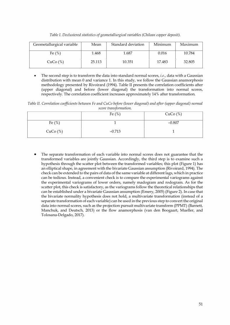
• The separate transformation of each variable into normal scores does not guarantee that the

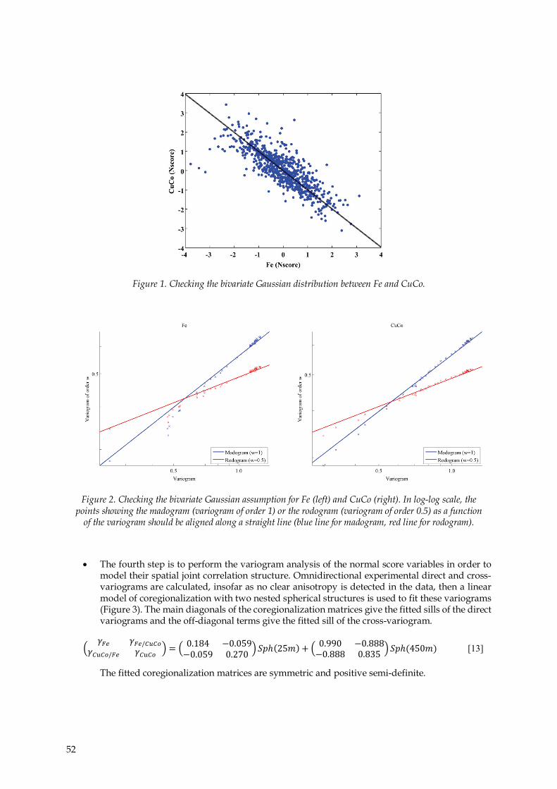
transformed variables are jointly Gaussian. Accordingly, the third step is to examine such a hypothesis through the scatter plot between the transformed variables; this plot (Figure 1) has an elliptical shape, in agreement with the bivariate Gaussian assumption (Rivoirard, 1994). The check can be extended to the pairs of data of the same variable at different lags, which in practice can be tedious. Instead, a convenient check is to compare the experimental variograms against the experimental variograms of lower orders, namely madogram and rodogram. As for the scatter plot, this check is satisfactory, as the variograms follow the theoretical relationships that can be established under a bivariate Gaussian assumption (Emery, 2005) (Figure 2). In case that the bivariate normality hypothesis does not hold, a multivariate transformation (instead of a separate transformation of each variable) can be used in the previous step to convert the original data into normal scores, such as the projection pursuit multivariate transform (PPMT) (Barnett, Manchuk, and Deutsch, 2013) or the flow anamorphosis (van den Boogaart, Mueller, and Tolosana-Delgado, 2017).

Fe (%) CuCo (%)

Fe (%) 1 –0.807

CuCo (%) –0.713 1

52

Figure 1. Checking the bivariate Gaussian distribution between Fe and CuCo.

Figure 2. Checking the bivariate Gaussian assumption for Fe (left) and CuCo (right). In log-log scale, the points showing the madogram (variogram of order 1) or the rodogram (variogram of order 0.5) as a function

of the variogram should be aligned along a straight line (blue line for madogram, red line for rodogram).

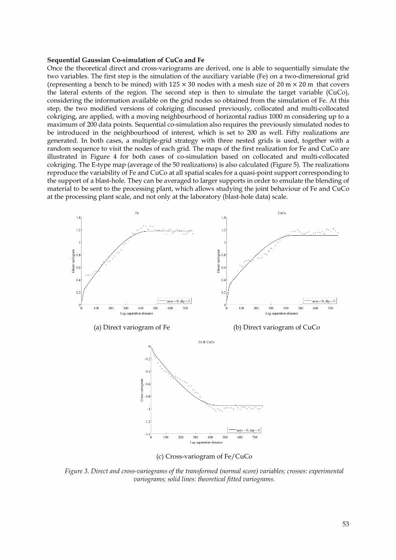
• The fourth step is to perform the variogram analysis of the normal score variables in order to model their spatial joint correlation structure. Omnidirectional experimental direct and cross-variograms are calculated, insofar as no clear anisotropy is detected in the data, then a linear model of coregionalization with two nested spherical structures is used to fit these variograms (Figure 3). The main diagonals of the coregionalization matrices give the fitted sills of the direct variograms and the off-diagonal terms give the fitted sill of the cross-variogram.

[13]

The fitted coregionalization matrices are symmetric and positive semi-definite.

53

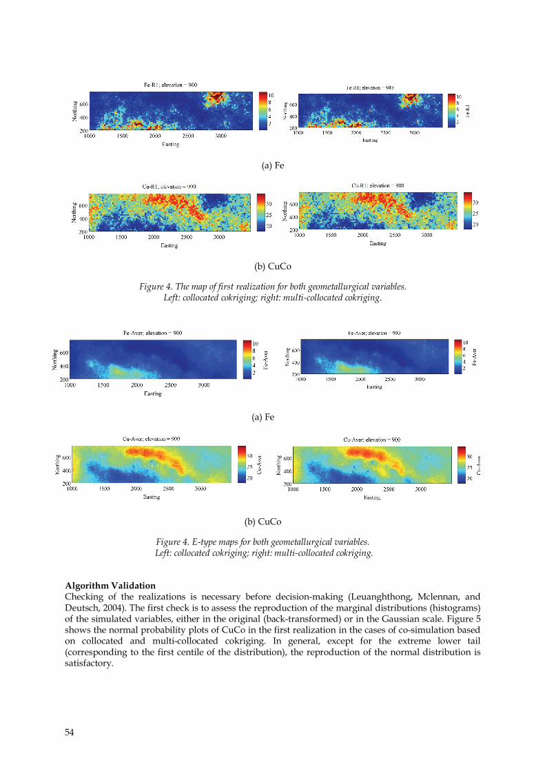
Sequential Gaussian Co-simulation of CuCo and Fe Once the theoretical direct and cross-variograms are derived, one is able to sequentially simulate the two variables. The first step is the simulation of the auxiliary variable (Fe) on a two-dimensional grid (representing a bench to be mined) with nodes with a mesh size of that covers the lateral extents of the region. The second step is then to simulate the target variable (CuCo), considering the information available on the grid nodes so obtained from the simulation of Fe. At this step, the two modified versions of cokriging discussed previously, collocated and multi-collocated cokriging, are applied, with a moving neighbourhood of horizontal radius 1000 m considering up to a maximum of 200 data points. Sequential co-simulation also requires the previously simulated nodes to be introduced in the neighbourhood of interest, which is set to 200 as well. Fifty realizations are generated. In both cases, a multiple-grid strategy with three nested grids is used, together with a random sequence to visit the nodes of each grid. The maps of the first realization for Fe and CuCo are illustrated in Figure 4 for both cases of co-simulation based on collocated and multi-collocated cokriging. The E-type map (average of the 50 realizations) is also calculated (Figure 5). The realizations reproduce the variability of Fe and CuCo at all spatial scales for a quasi-point support corresponding to the support of a blast-hole. They can be averaged to larger supports in order to emulate the blending of material to be sent to the processing plant, which allows studying the joint behaviour of Fe and CuCo at the processing plant scale, and not only at the laboratory (blast-hole data) scale.

(a) Direct variogram of Fe (b) Direct variogram of CuCo

(c) Cross-variogram of Fe/CuCo

Figure 3. Direct and cross-variograms of the transformed (normal score) variables; crosses: experimental variograms; solid lines: theoretical fitted variograms.

54

(a) Fe

(b) CuCo

Figure 4. The map of first realization for both geometallurgical variables. Left: collocated cokriging; right: multi-collocated cokriging.

(a) Fe

(b) CuCo

Figure 4. E-type maps for both geometallurgical variables. Left: collocated cokriging; right: multi-collocated cokriging.

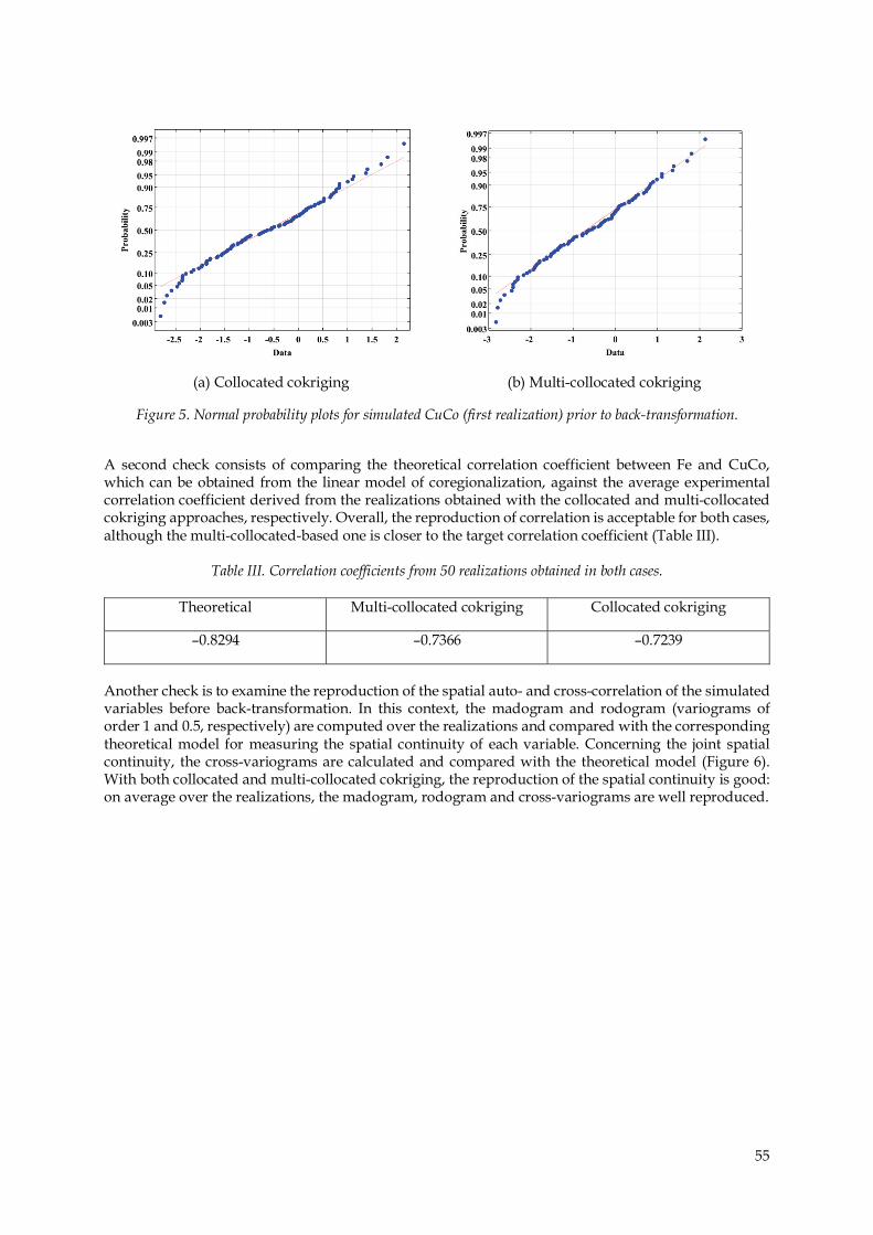
Algorithm Validation Checking of the realizations is necessary before decision-making (Leuanghthong, Mclennan, and Deutsch, 2004). The first check is to assess the reproduction of the marginal distributions (histograms) of the simulated variables, either in the original (back-transformed) or in the Gaussian scale. Figure 5 shows the normal probability plots of CuCo in the first realization in the cases of co-simulation based on collocated and multi-collocated cokriging. In general, except for the extreme lower tail (corresponding to the first centile of the distribution), the reproduction of the normal distribution is satisfactory.

55

(a) Collocated cokriging (b) Multi-collocated cokriging

Figure 5. Normal probability plots for simulated CuCo (first realization) prior to back-transformation.

A second check consists of comparing the theoretical correlation coefficient between Fe and CuCo, which can be obtained from the linear model of coregionalization, against the average experimental correlation coefficient derived from the realizations obtained with the collocated and multi-collocated cokriging approaches, respectively. Overall, the reproduction of correlation is acceptable for both cases, although the multi-collocated-based one is closer to the target correlation coefficient (Table III).

Table III. Correlation coefficients from 50 realizations obtained in both cases.

Theoretical Multi-collocated cokriging Collocated cokriging

–0.8294 –0.7366 –0.7239

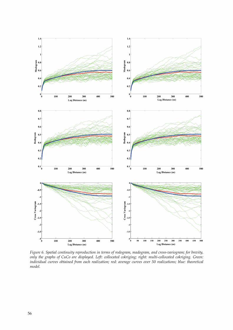
Another check is to examine the reproduction of the spatial auto- and cross-correlation of the simulated variables before back-transformation. In this context, the madogram and rodogram (variograms of order 1 and 0.5, respectively) are computed over the realizations and compared with the corresponding theoretical model for measuring the spatial continuity of each variable. Concerning the joint spatial continuity, the cross-variograms are calculated and compared with the theoretical model (Figure 6). With both collocated and multi-collocated cokriging, the reproduction of the spatial continuity is good: on average over the realizations, the madogram, rodogram and cross-variograms are well reproduced.

56

Figure 6. Spatial continuity reproduction in terms of rodogram, madogram, and cross-variogram; for brevity, only the graphs of CuCo are displayed. Left: collocated cokriging; right: multi-collocated cokriging. Green: individual curves obtained from each realization; red: average curves over 50 realizations; blue: theoretical model.

57

CONCLUSIONS The aim of this paper is to compare two implementations of sequential co-simulation for constructing block models that mimic the spatial distribution of geometallurgical variables. The case study shows that co-simulation built on either collocated or multi-collocated cokriging successfully reproduces the spatial correlation structure of the variables of interest, with a slight improvement for the multi-collocated implementation. This success can be explained by the large cokriging neighbourhood used to determine the successive conditional distributions (200 conditioning data points plus 200 previously simulated nodes) and by the particular coregionalization model of the geometallurgical variables, and may not be observed with other data or other neighbourhood sizes. The methodology proposed in this work is therefore of interest to validate the quality of the simulation. ACKNOWLEDGEMENTS The first author is grateful to Faculty Development Competitive Research Grants for 2018-2020 under contract no. 090118FD5336. The second author acknowledges funding of the Chilean Commission for Scientific and Technological Research (CONICYT), through grant CONICYT PIA Anillo ACT1407. REFERENCES Almeida, A.S. and Journel, A.G. (1994). Joint simulation of multiple variables with a Markov-type

coregionalization model. Mathematical Geology, 26 (5), 565-588.

Barnett, R.M., Manchuk, J.G., and Deutsch, C.V. (2013). Projection pursuit multivariate transform. Mathematical Geosciences, 46 (3), 337–359.

Boisvert, J.B., Rossi, M.E., Ehrig, K., and Deutsch, C.V. (2013). Geometallurgical modelling at Olympic Dam Mine, South Australia. Mathematical Geosciences, 45 (8), 1–25.

Chilès, J.P. and Delfiner, P., (2012). Geostatistics: Modeling Spatial Uncertainty. Wiley, New York.

Deutsch, C.V. (2013). Geostatistical modelling of geometallurgical variables – Problems and solutions. Proceedings of the second AusIMM International Geometallurgy Conference (Geomet 2013), Brisbane, Australia. Dominy, S. (ed.). Australasian Institute of Mining and Metallurgy, Melbourne. pp. 7-16.

Deutsch, C.V. and Journel, A.G. (1998). GSLIB: Geostatistical Software Library and User's Guide. Oxford University Press, New York.

Emery, X. (2004). Testing the correctness of the sequential algorithm for simulating Gaussian random fields. Stochastic Environmental Research and Risk Assessment, 18, 401–413.

Emery, X. (2005). Variograms of order ω: a tool to validate a bivariate distribution model. Mathematical Geology, 37 (2), 163—181.

Emery, X. (2008). A turning bands program for conditional co- simulation of cross-correlated Gaussian random fields. Computers & Geosciences, 34 (12), 1850–1862.

Emery, X. (2010). Iterative algorithms for fitting a linear model of coregionalization. Computers & Geosciences, 36 (9), 1150-1160.

Gómez-Hernández, J. (1991). A stochastic approach to the simulation of block conductivity fields conditioned upon data measured at a smaller scale. Doctoral dissertation, Stanford University, Stanford, CA.

58

Gómez-Hernández, J.J. and Cassiraga, E.F. (1994). Theory and practice of sequential simulation. Geostatistical Simulations. Armstrong, M. and Dowd, P.A. (eds). Kluwer, Dordrecht. pp. 111–124.

Gómez-Hernández, J.J. and Journel, A.G. (1993). Joint sequential simulation of multigaussian fields. Proceedings of Geostatistics Troia’92. Soares, A. (ed.). Springer, Dordrecht. pp. 85-94.

Goovaerts, P. (1997). Geostatistics for Natural Resources Evaluation. Oxford University Press, New York.

Goulard, M., Voltz, M. (1992). Linear coregionalization model: tools for estimation and choise of cross-variogram matrix. Mathematical Geology 24 (3), 269–286.

Hosseini, S.A. and Asghari, O. (2015). Simulation of geometallurgical variables through stepwise conditional transformation in Sungun copper deposit, Iran. Arabian Journal of Geosciences, 8, 3821–3831.

Journel, A.G. and Huijbregts, C.J. (1978). Mining Geostatistics. Academic Press, London.

Leuangthong, O., Mclennan, J.A., and Deutsch, C.V. (2004). Minimum acceptance criteria for geostatistical realizations. Natural Resources Research, 13 (3), 131–141.

Marcotte, D. (2012). Revisiting the linear model of coregionalization. Procedings of Geostatistics Oslo 2012. Abrahamsen, P., Hauge, R., and Kolbjornsen, O. (eds).,Springer, Dordrecht. pp. 67-78.

Paravarzar, S., Emery, X., and Madani, N. (2015). Comparing sequential Gaussian and turning bands algorithms for cosimulating grades in multi-element deposits, Comptes Rendus Geoscience, 347 (2), 84–93.

Rivoirard, J. (1994). Introduction to Disjunctive Kriging and Non-linear Geostatistics. Clarendon Press, Oxford.

Rondon, O. (2012). Teaching aid: minimum/maximum autocorrelation factors for joint simulation of attributes. Mathematical Geosciences, 44 (4), 469–504.

Rossi, M., Deutsch, C. V. (2014). Mineral Resource Estimation. Springer, Dordrecht.

Tran, T.T. (1994). Improving variogram reproduction on dense simulation grids. Computers & Geosciences, 20 (7–8), 1161–1168.

Van den Boogaart, K.G., Mueller, U., and Tolosana-Delgado, R. (2017). An affine equivariant multivariate normal score transform for compositional data. Mathematical Geosciences, 49 (2), 1–21.

Verly, G.W. (1993). Sequential Gaussian cosimulation: a simulation method integrating several types of information. Proceedings of Geostatistics Tróia ’92. Soare,s A. (ed.). Springer, Dordrecht. pp. 543-554.

Wackernagel, H. (2003). Multivariate Geostatistics: an Introduction with Applications. Springer, Berlin.

59

Nasser Madani Assistant Professor Nazarbayev University Dr Madani received a PhD in Mining Engineering from University of Chile, Santiago, Chile. Currently, he is an Assistant Professor at Nazarbayev University, where he teaches and conducts research on Geostatistics (linear, nonlinear, and multivariate). Prior to this position, Dr Madani was an Assistant Researcher at the Advanced Mining Technology Centre (AMTC), University of Chile, from 2013 to 2016, involved in modelling and evaluation of orebodies. He has consulted to the mining/petroleum companies and conducted research projects in geostatistical modelling, together with providing a practical knowledge for interpreting data from sampling, experiments, and industrial tests.

60